Article

Isobaric Vapor-Liquid Equilibrium of Biomass-Derived Ethyl Levulinate and Ethanol at 40.0, 60.0 and 80.0 kPa

by
Wenteng Bo
,
Xinghua Zhang
*,
Qi Zhang
,
Lungang Chen
,
Jianguo Liu
,
Longlong Ma
and
Shengyong Ma
School of Energy and Environment, Southeast University, Nanjing 211100, China
*
Author to whom correspondence should be addressed.
Energies 2025, 18(15), 3939; https://doi.org/10.3390/en18153939
Submission received: 4 July 2025 / Revised: 19 July 2025 / Accepted: 21 July 2025 / Published: 24 July 2025

Abstract

Isobaric vapor-liquid equilibrium (VLE) data for binary mixtures of biomass–derived ethyl levulinate and ethanol were measured using an apparatus comprising a modified Rose-Williams still and a condensation system. Measurements were taken at temperatures ranging from 329.58 K to 470.00 K and pressures of 40.0, 60.0 and 80.0 kPa. The thermodynamic consistency of the VLE data was evaluated using the Redlich-Kister area test, the Fredenslund test and the Van Ness point-to-point test. The data was correlated using three activity coefficient models: Wilson, NRTL and UNIQUAC. The Gibbs energy of mixing of the VLE data was analyzed to verify the suitability of the binary interaction parameters of these models. The activity coefficients and excess Gibbs free energy, calculated from the VLE experimental data and model correlation results, were analyzed to evaluate the models’ fit and the non–ideality of the binary system. The accuracy of the regression results was also assessed based on the root mean square deviation (RMSD) and average absolute deviation (AAD) for both temperature and the vapor phase mole fraction of ethyl levulinate. The results indicate that the NRTL model provided the best fit to the experimental data. Notably, the experimental data showed strong correlation with the predictions of all three models, suggesting their reliability for practical application.

1. Introduction

As a potential renewable biomass–derived platform compound, ethyl levulinate (EL) contains a carbonyl group and an ester group, which has good reactivity and can be subject to a variety of chemical reactions, such as hydrolysis, reduction, condensation, addition, etc. [1]. Taking advantages of the above reaction, EL can be used not only as fragrances, oil additives [2,3] and plasticizers [4] but also as an important pharmaceutical [5] and chemical raw material [6,7]. In addition, EL and its derivative γ-valerolactone can be used as a new type of liquid fuel additive, which is widely used in the field of petroleum alternative energy [8]. It was reported that the addition of appropriate amounts of EL to diesel fuel can improve power, environmental performance, and lubrication [9].
Currently, there are three methods for the preparation of ethyl levulinate EL: (1) esterification of levulinic acid, (2) catalytic alcoholysis of furfural alcohol in an ethanol solvent, and (3) direct alcoholysis of cellulose. The esterification of levulinic acid involves its reaction with ethanol to produce EL [10]. The catalytic alcoholysis uses furfural alcohol as the feedstock and synthesizes EL under acidic conditions through heating [11]. Direct alcoholysis of cellulose refers to the acid-catalyzed alcoholysis of cellulose in an ethanol solvent to produce EL [12].
Regardless of the method, impurities such as ethanol will remain in the reaction system, and high–purity EL can be obtained through separation processes such as distillation and extractive distillation [13]. And vapor-liquid equilibrium (VLE) data is required to design the separation process for production of high-purity EL. However, only Alexander J. Resk et al. [14] presented isothermal vapor-liquid equilibrium (VLE) values for EL + ethanol at a temperature of 60 °C and the isobaric VLE data at different temperatures is still lacking. Besides, the boiling point of EL is about 480 K at atmospheric pressure, and distillation under a reduced pressures can improve equipment safety and reduce energy consumption. Moreover, the chemical engineering data bank needs to be updated and improved with new experimental data to fit the model parameters. In conclusion, measuring the isobaric vapor-liquid equilibrium (VLE) data of the ethyl levulinate and ethanol under depressurized conditions is essential.
This work focuses on the isobaric vapor-liquid equilibrium data of EL + Ethanol at 40.0, 60.0 and 80.0 kPa, with the aim of providing fundamental references and equilibrium data for industrial production. All VLE data were subjected to thermodynamic consistency tests, including the Redlich-Kister area test, the Fredenslund test and the Van Ness point-to-point test. Three activity coefficient models, Wilson, nonrandom two–liquid (NRTL), and universal quasichemical activity coefficient (UNIQUAC) were employed to correlate the experimental data of the binary system.

2. Experimental and/or Computational Methods

2.1. Chemicals

The chemicals of ethanol, cyclohexanone and ethyl levulinate were analytical grade and obtained from commercial sources. The relevant information is exhibited in Table 1. The mass fractions of the chemicals were analyzed and confirmed using GC (gas chromatography), and no detectable impurity was observed. Therefore, all the reagents were utilized without any further purification. The boiling temperatures were measured with mercury thermometers, as presented in Table 1. The differences in boiling temperatures ( T b ) between the reference data and experimental data are all within 0.1 K.

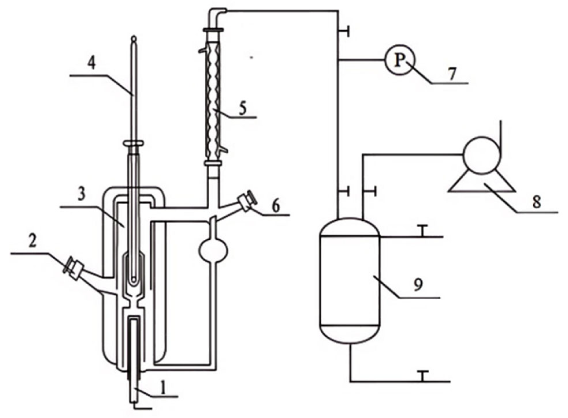
2.2. Apparatus and Procedure

The isobaric vapor-liquid equilibrium experiments were carried out in a set of apparatus, as illustrated in Figure 1, which included a modified Rose-Williams still [16,17] and a condensation system. The still could ensure intimate and continuous contact of the vapor and liquid phases to establish phase equilibrium in a short time. The total volume of the still was about 160 cm3 with around 80 cm3 occupied by the liquid solution. The solutions were prepared gravimetrically by an Sartorius BCE224-1CCN electronic balance, with a precision of 0.1 mg. The energy supplied to the still is generated by a heating rod, with its voltage regulated by a transformer at a rate of (5~10 V)/(10~15 min). The coolant in the condensation system is composed of water and ethylene glycol in a mass ratio of 2:1, with the temperature set at 263 K to facilitate the rapid condensation of vapor into liquid, allowing it to return to the equilibrium chamber efficiently. All temperature measurements were obtained using a high-precision mercury thermometer, which had an uncertainty of 0.04 K. The pressure control of the set of apparatus was managed by a Liquid ring vacuum pump and a buffer tank with a capacity of 20 L. The Liquid ring vacuum pump operated continuously, while the amount of air entering the system was controlled by adjusting the valve connecting the buffer tank to the outside, which could regulate the pressure of the still to the set value of reduced pressure conditions and ensure the pressure of the entire system stable for a long time. A U-tube differential manometer was connected between the condenser and the buffer tank, with its uncertainty of 0.1 kPa to precisely measure the pressure. To ensure that all experiments reached phase equilibrium, the vapor and liquid samples were analyzed until the temperatures stabilized for more than 2 h. After equilibrium was attained, samples from both the vapor (chilled to liquid form) and liquid phases were extracted through the sampling ports. A micro-syringe was utilized to withdraw these samples, followed by three parallel tests of each sample using gas chromatography (GC).
The isobaric vapor-liquid equilibrium data for the cyclohexanone + ethanol binary system, which also contains ethanol, were measured at 101.3 kPa and compared with data from the literature to verify the reliability of the apparatus shown in Figure 2.
The results demonstrated that the isobaric VLE data for the binary system of Cyclohexanone + Ethanol at 101.3 kPa exhibited excellent agreement with reference data, thereby validating the reliability of the set of apparatus.

2.3. Analysis

The equilibrium compositions of the vapor (chilled to liquid form) and liquid phases were determined using a SHIMADZU GC-2014C equipped with a flame ionization detector (FID). A FFAP capillary column (30m × 0.32 mm × 0.25 μm) was used to effectively separate various components present in the sample, including ethanol. The carrier gas was high–purity nitrogen (≥99.999%) flowing at a rate of 30 mL·min−1. The flow rates of hydrogen (≥99.999%) and air (≥99.99%) were 40 mL·min−1 and 400 mL·min−1, respectively. The temperatures of column, injector and detector were (363.15 K for 2 min then at 20 K/min rise to 483.15 K for 2 min, 513.15 K and 523.15 K). An injection volume of 0.8 μL was used for each sample in the GC analysis. The GC response peaks were analyzed in the LabSolutions chromatography station and the area correction normalization method was adopted for component quantitative analysis, obtaining the composition results of the vapor and liquid phase samples in the binary system. The GC was calibrated with standard solutions prepared gravimetrically by the electronic balance. For the binary system of ethyl levulinate + ethanol, five standard solutions with different mass ratios were prepared according to the gradient, and the corresponding peak area ratios were obtained by GC analysis (each standard solution was analyzed three times to ensure accuracy). The expressions of the calibration curves, the correlation coefficients R2 and the relative mass correction factors were obtained by fitting the data points in Origin 2021 and are shown in Figure S1 provided in the Supplementary Materials. The uncertainties of the liquid–phase and vapor-phase mole fractions were both kept within 0.0003, ensuring the reliability of the results.

3. Results and Discussion

3.1. Vapor-Liquid Equilibrium Data

Isobaric vapor-liquid equilibrium (VLE) data for the binary system of EL (1) + Ethanol (2) at pressures of 40.0, 60.0 and 80.0 kPa were generated using the modified Rose-Williams still, and are presented in Table 2. The listed VLE data comprised: T (equilibrium temperature), xi and yi (mole fractions of the liquid and vapor phases, respectively), γi (activity coefficient), ln(γ12) (used for thermodynamic consistency test), gE (dimensionless excess Gibbs free energy of the mixture), gM,V and gM,L (dimensionless Gibbs energy of mixing functions for the vapor and liquid phases, respectively).
For isobaric VLE data, the general expression is given in Equation (1) [19]:
P y i ϕ i v ^ = P i s ϕ i s γ i x i e x p [ V i L ( P P i s ) R T ]
where i represents the different components, P and P i s are the total system pressure and the saturated vapor pressure, respectively, ϕ i v and ϕ i s are the fugacity coefficient of the vapor phase and pure component i at pressure P i s and T, respectively, xi, yi and γi have the same meaning as above; V i L is the liquid mole volume. In addition, P i s refers to the saturated pressure at the equilibrium temperature, and is calculated using the extended Antoine equation, which is presented as [20]:
ln ( P i s , k P a ) = C 1 i + C 2 i T + C 3 i + C 4 i T + C 5 i ln T + C 6 i T C 7 i C 8 i T C 9 i
Each component’s Antoine constants were given by Aspen Plus V11 and listed in Table 3.
At low pressure, the vapor phase can be considered as an ideal gas, the Poynting factor e x p [ V i L ( P P i s ) / R T ] , ϕ i v and ϕ i s can be considered as 1, and then Equation (1) can be expressed as:
P y i ^ = P i s γ i x i
So, γi is calculable from Equation (3) and reported in Table 2. The experimental data indicates that the activity coefficients of EL and Ethanol in the vapor-liquid equilibrium system are greater than or equal to one at 40.0, 60.0 and 80.0 kPa. This suggests that the binary system exhibits significant positive deviation from ideal behavior, and that there may be strong interaction between the two components. Furthermore, as the molar fraction of EL increases in the liquid phase, the activity coefficient of EL decreases while the activity coefficient of Ethanol increases. However, at high concentrations of EL, the activity coefficient of Ethanol shows a decreasing trend. This behavior can be attributed to the intermolecular interactions between ethyl levulinate and ethanol.
The dimensionless excess Gibbs free energy gE was calculated based on the experimental VLE data to reflect the difference between the actual solution and the ideal solution under identical conditions of temperature, pressure and composition. And gE is given by Equation (4) [21]:
g E = G E R T = x 1 ln γ 1 + x 2 ln γ 2
And gE for the binary system of EL (1) + Ethanol (2) at pressures of 40.0, 60.0 and 80.0 kPa are listed in Table 2. It can be observed that gE of the mixture deviates positively from ideal behavior at all three pressures, which is consistent with Raoult’s law. Additionally, as the mole fraction of EL in the liquid phase increases, gE shows a trend of initially increasing and then decreasing.

3.2. Thermodynamic Consistency Tests

During the data measurement process, errors, both large and small, are inevitably introduced in the vapor-liquid equilibrium data. To evaluate the reliability of the experimental results, thermodynamic consistency tests are essential. As summarized by Jaime Wisniak et al. [22], the Redlich-Kister area test [23], the Fredenslund test [24] and the Van Ness point-to-point test [25] were used to assess the quality of the VLE data in this study.
For the Redlich-Kister area test, the underlying principle is the Gibbs-Duhem equation, which describes the thermodynamic relationship between activity coefficients and composition in binary mixtures:
x 1 = 0 x 1 = 1 ln γ 1 γ 2 d x 1 = T x 1 = 0 T x 1 = 1 H E R T 2 d T + P x 1 = 0 P x 1 = 1 V E R T d P
Under isobaric conditions, the second term on the right side of Equation (5) is equal to 0. And considering the enthalpy effects of mixing, the data set is regarded as thermodynamically consistent when the following condition is satisfied:
D = 100 0 1 ln γ 1 γ 2 d x 1 0 1 ln γ 1 γ 2 d x 1 = 100 A + A A + + A 2
Applying the Redlich-Kister area test to binary vapor-liquid equilibrium (VLE) data involves plotting ln(γ12) against the mole fraction x1, resulting in a semi-logarithmic plot commonly referred to as the Redlich-Kister plot. In this plot, areas A+ and A represent the regions enclosed between the curve and axis above and below the x-axis, respectively. It is important to note that the Redlich-Kister test is applicable exclusively to binary mixtures.
In this work, the Redlich-Kister plots for the binary system of EL (1) + Ethanol (2) at all pressures are shown in Figure 3. And the values of D at 40.0, 60.0 and 80.0 kPa are 1.36, 1.04 and 0.33, respectively, all of which are less than 2. These results demonstrate that the experimental VLE data satisfy the thermodynamic consistency criteria according to the Redlich-Kister area test.
For the Fredenslund test, the dimensionless excess Gibbs free energy gE obtained from Equation (4) is correlated using a series of Legendre polynomials:
g E = G E R T = x 1 x 2 k = 0 n a k L k x 1 k = 0 , 1 , , n
where n is the degree of the polynomial used, and a k is the parameter of the Legendre orthogonal polynomial, which is shown in Equation (8):
L k x 1 = 2 k 1 2 x 1 1 L k 1 x 1 k 1 L k 2 x 1 / k
with L 0 x 1 = 1 and L 1 x 1 = 2 x 1 1 as the first two Legendre polynomials. The dimensionless excess Gibbs free energy gE describes the relationship between the deviation of the components and the deviation of the solution:
ln γ 1 = g E + x 2 d g E d x 1
The pertinent activity coefficients (γ1) can be calculated from Equation (9), and then the mole fraction of the vapor phase (y1) can be determined based on the VLE expression (Equation (3)). As stated by Fredenslund, a set of P-T-x1-y1 data is considered consistent if the average absolute deviation between y1 is below 0.01 units, which is
y 1 = 1 N i = 1 N y 1 , i e x p y 1 , i c a l 0.01
where N is the number of data points at a specific pressure.
Typically, a Legendre series with three to five terms is sufficient to determine the accuracy of the data. In this work, gE was correlated using a four-term Legendre polynomial, and the values of y1 at 40.0, 60.0 and 80.0 kPa are 0.00014, 0.00005 and 0.00013, respectively, all of which are less than 0.01. Meanwhile, residuals of the equilibrium temperatures
T = T i e x p T i c a l
obtained by correlating the activity coefficient model, are listed in Table 4, Tables S2 and S3, with the distribution plots shown in Figure 4, Figure 5 and Figure 6. The residuals in these plots exhibit random behavior, indicating that the isobaric VLE data satisfy the Fredenslund test.
For the Van Ness point-to-point test, the work of Van Ness in 1995 demonstrated that the application of the Van Ness point-to-point test involves calculating the value of ln(γ12) for each data point, comparing them with the calculated values obtained by fitting the activity coefficient model, and analyzing the residual distribution of ln(γ12):
ln γ 1 / γ 2 = ln γ 1 e x p / γ 2 e x p ln γ 1 c a l / γ 2 c a l
If the residuals are randomly distributed, the set of data is considered consistent.
In this work, the residuals of ln(γ12) are listed in Table 4, Tables S2 and S3, with the distributions shown in Figure 4, Figure 5 and Figure 6, which exhibit distinct random behavior, indicating that the isobaric VLE data satisfy the Van Ness point-to-point test.
Given that both the Fredenslund and Van Ness point-to-point tests rely on comparing experimental data with model-predicted values, a certain level of model dependency is inevitably introduced into the assessment.

3.3. Data Correlation

The experimental VLE data for the binary system of EL (1) + Ethanol (2) at 40.0, 60.0 and 80.0kPa was fitted by the Wilson [26], NRTL [27] and UNIQUAC [28] models, which was carried out using Aspen Plus V11.0. A. Marcilla et al. [29] suggested that the necessity of considering the temperature dependence of the model parameters can be detected prior to the correlation process by analyzing the Gibbs energy of mixing of the experimental VLE data. For a binary isobaric vapor-liquid equilibrium system, when the vapor phase is treated as an ideal gas, the dimensionless Gibbs energy of mixing of the vapor and liquid phases (gM,V and gM,L) can be expressed as follows:
g M , V = G M , V R T = y 1 ln y 1 P P 1 s + y 2 ln y 2 P P 2 s
g M , L = x 1 y 1 ln y 1 P 2 s y 2 P 1 s + g M , V
where P and P i s are the total system pressure and the saturated vapor pressure of the pure component i, respectively.
The calculated gM,V and gM,L are listed in Table 2, with the corresponding vapor and liquid gM curves shown in Figure 7 and Figure S2. The horizontal axis is represented by the mole fraction of the light component (x2, y2) to ensure consistency. The tie-lines connecting the Gibbs energy of mixing of the conjugated vapor and liquid phases are close to being tangent to the smooth gM,L curve, which connects all gM,L at different temperatures. Therefore, consistent and good (near the experimental data) fitting results can be achieved without any temperature dependence in the model according to A. Marcilla.
However, the temperature range for the binary VLE system of EL + Ethanol is quite large. To ensure the accuracy of fitting, temperature dependence is appropriately introduced into the relevant model parameters. The corresponding equations are presented in Table 5. For the NRTL model, the nonrandomness parameter (αij) was fixed at 0.3, as recommended in Aspen Plus.
The interaction parameters for the thermodynamic models were determined using the maximum likelihood principle. The objective function is expressed as follows:
O F = i = 1 N T i e x p T i c a l σ T 2 + P i e x p P i c a l σ P 2 + x i e x p x i c a l σ x 2 + y i e x p y i c a l σ y 2
The objective function is to minimize the differences of experimental (exp) and calculated (cal) values of T, P, xi, and yi. σ denotes standard deviation, and N denotes the experimental data number.
The correlation results of each activity coefficient model, including the calculated VLE data, residual analysis, activity coefficients, and dimensionless excess Gibbs free energy, are listed in Table 4 (Wilson), Table S2 (NRTL) and Table S3 (UNIQUAC).
The T-x-y diagrams for the binary system of EL (1) + Ethanol (2) at 40.0, 60.0, and 80.0 kPa are presented in Figure 8, with the y-x diagrams shown in Figure 9. As shown in the figures, no azeotrope is observed for the EL and ethanol system at 40.0, 60.0, and 80.0 kPa. For the binary system, the fitting deviations of all three models are quite small. The curves of all three models smoothly pass through the experimental points at all pressures, and the curves nearly coincide, indicating that all three models exhibit a good correlation with the experimental vapor-liquid equilibrium data.
The inset in Figure 9 shows that as the pressure decreases, the y-x curve deviates further from the main diagonal. This suggests that lowering the equilibrium pressure is beneficial for the separation of ethyl levulinate and ethanol. Overall, the effect of this improvement is not significant.
The γi-x1 and gE-x1 diagrams for the binary system are shown in Figure 10 and Figure 11, respectively. All the activity coefficients and the dimensionless excess Gibbs free energy were calculated from the correlation results of the Wilson model using Equation (3) and (4). The calculated results are generally consistent with the experimental measurements, further confirming the applicability of the activity coefficient model. Moreover, at lower pressures, the activity coefficients of EL and ET are smaller, and the dimensionless excess Gibbs free energy is also smaller, indicating that the binary system deviates less from the ideal state. This behavior may be attributed to the polarity difference between EL and ethanol.
The root mean square deviation (RMSD) and average absolute deviation (AAD) of the VLE data for the three models were computed to assess the correlation. The expressions for RMSD and AAD are given as follows:
R M S D T = i = 1 N T i e x p T i c a l 2 N 0.5
R M S D y 1 = i = 1 N y 1 i e x p y 1 i c a l 2 N 0.5
A A D T = 1 N i = 1 N T i e x p T i c a l
g E = G E R T = x 1 ln γ 1 + x 2 ln γ 2
A A D y 1 = 1 N i = 1 N y 1 i e x p y 1 i c a l
Table 6 presents the correlated parameters for the three models, along with the RMSDs and AADs for the equilibrium temperature and vapor mole fraction. For the binary system of EL (1) + Ethanol (2) at 40.0, 60.0 and 80.0kPa, the RMSDmax (y1) = 0.0003, the AADmax (y1) = 0.0002, the RMSDmax (T) = 0.05 K and the AADmax (T) = 0.04 K. The RMSD (y1) and AAD (y1) < 0.001. RMSD (T) and AAD (T) < 0.1 K. The deviations were relatively small and fell within the acceptable error range. Based on the results, the Wilson, NRTL and UNIQUAC models provided accurate correlations of the experimental data, exhibiting similar levels of accuracy.

4. Conclusions

The isobaric VLE data of EL + Ethanol was measured using an apparatus that included a modified Rose-Williams still and a condensation system, operating at pressures of 40.0, 60.0 and 80.0 kPa. The VLE data passed the Redlich-Kister area test, the Fredenslund test and the Van Ness point-to-point test, confirming its thermodynamic consistency. For the systems of EL + Ethanol at all pressures, the Wilson, NRTL and UNIQUAC activity coefficient models were all successfully correlated with the VLE data. The curves of all three models on the T-x-y plot smoothly pass through the experimental points and are almost coincided. The analysis of the Gibbs energy of mixing for the VLE data shows that the binary interaction parameters have weak temperature dependence. The RMSD (y1) and AAD (y1) values were less than 0.001, while the RMSD (T) and AAD (T) values were less than 0.1 K. These results indicated that the experimental data is reliable. The generated VLE data can be used to design the separation processes for ethyl levulinate and ethanol in the material product system. The binary interaction parameters obtained from the regression using three local composition activity coefficient models—Wilson, NRTL, and UNIQUAC—are not only applicable to binary systems, but can also be extended to multicomponent systems containing ethyl levulinate and ethanol. Moreover, the VLE data obtained in this study may serve as a useful reference for similar binary systems, such as methyl levulinate and methanol. In addition, the variations of the activity coefficients and excess Gibbs free energy for the EL + Ethanol system reveal the interaction between ethyl levulinate and ethanol, as well as the system’s positive deviation characteristics. In future studies, it is recommended to conduct additional vapor-liquid equilibrium experiments over a wider range of pressures and with other levulinate ester−alcohol systems, in order to further validate the applicability of thermodynamic models and to improve the thermodynamic database for levulinate ester compounds.

Supplementary Materials

The following supporting information can be downloaded at: https://www.mdpi.com/article/10.3390/en18153939/s1, The calculation methods for the uncertainty of measured variables; Table S1: Vapor-liquid Equilibrium (VLE) Data for the Binary System of Cyclohexanone(1) + Ethanol (2); Table S2: Calculation of VLE Data (T-x-y), Activity Coefficients (γi), Dimensionless Excess Gibbs Free Energy (gE), ΔT and Δln(γ12) Using the NRTL Model for the EL (1) + Ethanol (2) System at 40.0, 60.0 and 80.0 kPa; Table S3: Calculation of VLE Data (T-x-y), Activity Coefficients (γi), Dimensionless Excess Gibbs Free Energy (gE), ΔT and Δln(γ12) Using the UNIQUAC Model for the EL (1) + Ethanol (2) System at 40.0, 60.0 and 80.0 kPa; Figure S1: Gas chromatography calibration curves of the two binary systems; Figure S2: Representation of the straight lines that connect the conjugated vapor and liquid phases for the binary system of EL (1) + Ethanol (2) and are tangent to the gM,L curve; The calculation of mole fraction from GC areas.

Author Contributions

Conceptualization, W.B., X.Z. and S.M.; methodology, W.B. and S.M.; investigation, W.B.; data curation, W.B.; writing—original draft preparation, W.B.; writing—review and editing, W.B., X.Z. and Q.Z.; supervision, L.C. and J.L.; resources, L.M.; funding acquisition, L.M. All authors have read and agreed to the published version of the manuscript.

Funding

This work was funded by grants from the National Natural Science Foundation of China (Nos. 52236010, 52376173), Jiangsu Provincial Double−Innovation Doctor Program (No. JSSCBS20220178), and the Fundamental Research Funds for the Central Universities (No. 2242022R10058).

Data Availability Statement

The original contributions presented in this study are included in the article/Supplementary Materials. Further inquiries can be directed to the corresponding authors.

Conflicts of Interest

The authors declare no conflicts of interest.

References

  1. Ghosh, M.K.; Howard, M.S.; Zhang, Y.; Djebbi, K.; Capriolo, G.; Farooq, A.; Curran, H.J.; Dooley, S. The combustion kinetics of the lignocellulosic biofuel, ethyl levulinate. Combust. Flame 2018, 193, 157–169. [Google Scholar] [CrossRef]
  2. Api, A.M.; Belsito, D.; Botelho, D.; Bruze, M.; Burton, G.A., Jr.; Buschmann, J.; Dagli, M.L.; Date, M.; Dekant, W.; Deodhar, C.; et al. RIFM fragrance ingredient safety assessment, ethyl levulinate, CAS Registry Number 539-88-8. Food Chem. Toxicol. 2019, 127 (Suppl. 1), S48–S54. [Google Scholar] [CrossRef] [PubMed]
  3. Unlu, D.; Boz, N.; Ilgen, O.; Hilmioglu, N. Improvement of fuel properties of biodiesel with bioadditive ethyl levulinate. Open Chem. 2018, 16, 647–652. [Google Scholar] [CrossRef]
  4. Ren, J.; Zhang, Y.; Quan, Y. Preparation of Ethyl Levulinate by Sulfonating Active Carbon Catalytic Furfuryl Alcohol Alcoholysis Used as Plasticizer, Involves Dissolving Activated Carbon Powder in Deionized Water, Adding Concentrated Sulfuric Acid, and Placing Furfuryl Alcohol, Sulfonated Activated Carbon Catalyst, and Ethanol. CN118307401-A, 9 April 2024. [Google Scholar]
  5. Muzzio, M.; Yu, C.; Lin, H.; Yom, T.; Boga, D.A.; Xi, Z.; Li, N.; Yin, Z.; Li, J.; Dunn, J.A.; et al. Reductive amination of ethyl levulinate to pyrrolidones over AuPd nanoparticles at ambient hydrogen pressure. Green Chem. 2019, 21, 1895–1899. [Google Scholar] [CrossRef]
  6. Gomes, G.R.; Breitkreitz, M.C.; Pastre, J.C. Ash influence on the ethyl levulinate production from sugarcane molasses mediated by taurine hydrogen sulfate. Acs Sustain. Chem. Eng. 2021, 9, 13438–13449. [Google Scholar] [CrossRef]
  7. Hamryszak, L.; Grzesik, M. Levulinic esters. Production, application and kinetic studies. Przem. Chem. 2017, 96, 327–331. [Google Scholar]
  8. Khalid, M.; Mesa, M.G.; Scapens, D.; Osatiashtiani, A. Advances in sustainable γ-Valerolactone (GVL) production via catalytic transfer hydrogenation of levulinic acid and its esters. Acs Sustain. Chem. Eng. 2024, 12, 16494–16517. [Google Scholar] [CrossRef]
  9. Bhonsle, A.K.; Faujdar, E.; Rawat, N.; Singh, R.K.; Singh, J.; Trivedi, J.; Atray, N. Synthesis and characterization of novel ethyl levulinate coupled N-phenyl-p-phenylenediamine multifunctional additive: Oxidation stability and lubricity improver in biodiesel. Energy Sources Part A-Recovery Util. Environ. Eff. 2022, 44, 6236–6248. [Google Scholar] [CrossRef]
  10. Pasha, N.; Lingaiah, N.; Shiva, R. Zirconium exchanged phosphotungstic acid catalysts for esterification of levulinic acid to ethyl levulinate. Catal. Lett. 2019, 149, 2500–2507. [Google Scholar] [CrossRef]
  11. Li, M.; Wei, J.; Yan, G.; Liu, H.; Tang, X.; Sun, Y.; Zeng, X.; Lei, T.; Lin, L. Cascade conversion of furfural to fuel bioadditive ethyl levulinate over bifunctional zirconium-based catalysts. Renew. Energy 2020, 147, 916–923. [Google Scholar] [CrossRef]
  12. Zhao, W.; Wang, B.; Zhang, W. Research progress in preparation of ethyl levulinate from cellulose. Mod. Chem. Ind. 2024, 44, 44–49, 54. [Google Scholar]
  13. Huang, Z.; Yuan, H. Research advances on preparation of ethyl levulinate through alcoholysis of biomass and its derivatives. Mod. Chem. Ind. 2021, 41, 42–46. [Google Scholar]
  14. Resk, A.J.; Peereboom, L.; Kolah, A.K.; Miller, D.J.; Lira, C.T. Phase equilibria in systems with levulinic acid and ethyl levulinate. J. Chem. Eng. Data 2014, 59, 1062–1068. [Google Scholar] [CrossRef]
  15. Wang, X.; Zhuang, X.; Yun, S.; Chen, J.; Jiang, D. Measurement and correlation of vapor-liquid equilibrium for a cyclohexene-cyclohexanol binary system at 101.3 kPa. Chin. J. Chem. Eng. 2011, 19, 484–488. [Google Scholar] [CrossRef]
  16. Yang, C.; Sun, Y.; Qin, Z.; Feng, Y.; Zhang, P.; Feng, X. Isobaric vapor-liquid equilibrium for four binary systems of ethane-1,2-diol, butane-1,4-diol, 2-(2-Hydroxyethoxy)ethan-1-ol, and 2- 2-(2-Hydroxyethoxy)ethoxy ethanol at 10.0 kPa, 20.0 kPa, and 40.0 kPa. J. Chem. Eng. Data 2014, 59, 1273–1280. [Google Scholar] [CrossRef]
  17. Mi, X.; Yang, C.; Sun, F.; Li, B. Vapor-liquid equilibrium for the binary of propylene glycol methyl ether acetate plus ethyl lactate and propylene glycol methyl ether plus ethyl lactate at 101.3 and 20.0 kPa. J. Chem. Eng. Data 2021, 66, 146–153. [Google Scholar] [CrossRef]
  18. Zhang, K.; Xu, D.; Zhou, Y.; Shi, P.; Gao, J.; Wang, Y. Isobaric vapor-liquid phase equilibrium measurements, correlation, and prediction for separation of the mixtures of cyclohexanone and alcohols. J. Chem. Eng. Data 2018, 63, 2038–2045. [Google Scholar] [CrossRef]
  19. Wang, Y.; Zhang, H.; Pan, X.; Yang, J.; Cui, P.; Zhang, F.; Gao, J. Isobaric vapor-liquid equilibrium of a ternary system of ethyl acetate plus propyl acetate plus dimethyl sulfoxide and binary systems of ethyl acetate plus dimethyl sulfoxide and propyl acetate plus dimethyl sulfoxide at 101.3 kPa. J. Chem. Thermodyn. 2019, 135, 116–123. [Google Scholar] [CrossRef]
  20. De La Calle-Arroyo, C.; Lopez-Fidalgo, J.; Rodriguez-Aragon, L.J. Optimal designs for Antoine Equation. Chemom. Intell. Lab. Syst. 2021, 214, 104334. [Google Scholar] [CrossRef]
  21. Kumar, R.V.; Rao, M.A.; Rao, M.V.; Prasad, D.H.L. Activity coefficient and excess Gibbs free energy of allyl alcohol with tetrachloroethylene. Phys. Chem. Liq. 1997, 35, 121–126. [Google Scholar] [CrossRef]
  22. Wisniak, J.; Ortega, J.; Fernández, L. A fresh look at the thermodynamic consistency of vapour-liquid equilibria data. J. Chem. Thermodyn. 2017, 105, 385–395. [Google Scholar] [CrossRef]
  23. Redlich, O.; Kister, A.T. Thermodynamics of nonelectrolyte solutions-X-Y-T relations in a binary system. Ind. Eng. Chem. 1948, 40, 341–345. [Google Scholar] [CrossRef]
  24. Fredenslund, A.; Gmehling, J.; Rasmussen, P. Vapor-Liquid Equilibria Using Unifac, 1st ed.; Elsevier: Amsterdam, The Netherlands, 1977; pp. 198–226. [Google Scholar]
  25. Vanness, H.C. Thermodynamics in the treatment of vapor-liquid-equilibriu (VLE) data. Pure Appl. Chem. 1995, 67, 859–872. [Google Scholar] [CrossRef]
  26. Pazuki, G.R.; Taghikhani, V.; Vossoughi, M. Correlation and prediction the activity coefficients and solubility of amino acids and simple peptide in aqueous solution using the modified local composition model. Fluid Phase Equilibria 2007, 255, 160–166. [Google Scholar] [CrossRef]
  27. Winter, B.; Winter, C.; Esper, T.; Schilling, J.; Bardow, A. SPT-NRTL: A physics-guided machine learning model to predict thermodynamically consistent activity coefficients. Fluid Phase Equilibria 2023, 568, 113731. [Google Scholar] [CrossRef]
  28. Bakhshi, H.; Mobalegholeslam, P. A modification of UNIQUAC model for electrolyte solutions based on the local composition concept. J. Solut. Chem. 2020, 49, 1485–1496. [Google Scholar] [CrossRef]
  29. Marcilla, A.; Olaya, M.M.; Reyes-Labarta, J.A. The unavoidable necessity of considering temperature dependence of the liquid Gibbs energy of mixing for certain VLE data correlations. Fluid Phase Equilibria 2018, 473, 17–31. [Google Scholar] [CrossRef]
Figure 1. VLE apparatus used in this work: 1, heating rod; 2, liquid phase sampling port; 3, vapor-liquid balance chamber; 4, mercury thermometer; 5, condenser; 6, vapor phase sampling port; 7, U-tube differential manometer; 8, Liquid ring vacuum pump; 9, buffer tank.
Energies 18 03939 g001
Figure 2. T-x-y diagram for the Cyclohexanone (1) + Ethanol (2) at 101.3 kPa: circle, from the experiment data; triangle up from the ref. [18] data.
Energies 18 03939 g002
Figure 3. The Redlich-Kister plots for the binary system of EL (1) + Ethanol (2) at: (a) 40.0 kPa; (b) 60.0 kPa; (c) 80.0 kPa.
Energies 18 03939 g003
Figure 4. The residual distribution for the binary system of EL (1) + Ethanol (2) at 40.0 kPa: (a) residuals of equilibrium temperatures; (b) residuals of ln(γ12).
Energies 18 03939 g004
Figure 5. The residual distribution for the binary system of EL (1) + Ethanol (2) at 60.0 kPa: (a) residuals of equilibrium temperatures; (b) residuals of ln(γ12).
Energies 18 03939 g005
Figure 6. The residual distribution for the binary system of EL (1) + Ethanol (2) at 80.0 kPa: (a) residuals of equilibrium temperatures; (b) residuals of ln(γ12).
Energies 18 03939 g006
Figure 7. Representation of the straight lines that connect the conjugated vapor and liquid phases for the binary system of EL (1) + Ethanol (2) at 40.0 kPa and are tangent to the gM,L curve.
Energies 18 03939 g007
Figure 8. The T-x-y diagrams for the binary system of EL (1) + Ethanol (2) at 40.0, 60.0, and 80.0 kPa. The solid black squares, solid red circles, and solid blue triangles represent the experimental molar fractions of EL in the liquid phase at 40.0, 60.0, and 80.0 kPa, respectively. The open black squares, open red circles, and open blue triangles represent the experimental molar fractions of EL in the vapor phase at 40.0, 60.0, and 80.0 kPa, respectively. The solid black, red, and blue lines represent the values calculated using the Wilson model. The dashed black, red, and blue lines represent the values calculated using the NRTL model. The dash-dot black, red, and blue lines represent the values calculated using the UNIQUAC model.
Energies 18 03939 g008
Figure 9. The y-x diagrams for the binary system of EL (1) + Ethanol (2) at 40.0, 60.0, and 80.0 kPa. The solid black squares, solid red circles, and solid blue triangles represent the experimental molar fractions of EL in the vapor phase at 40.0, 60.0, and 80.0 kPa, respectively. The solid black, red, and blue lines represent the values calculated using the Wilson model. The dashed black, red, and blue lines represent the values calculated using the NRTL model. The dash-dot black, red, and blue lines represent the values calculated using the UNIQUAC model.
Energies 18 03939 g009
Figure 10. The γi-x1 diagrams for the binary system of EL (1) + Ethanol (2) at 40.0, 60.0, and 80.0 kPa. The solid black squares, solid red circles, and solid blue triangles represent the activity coefficient of ethyl levulinate at 40.0, 60.0, and 80.0 kPa, respectively. The open black squares, open red circles, and open blue triangles represent the activity coefficient of Ethanol at 40.0, 60.0, and 80.0 kPa, respectively. The curves represent the calculated results with correlation of the Wilson model.
Energies 18 03939 g010
Figure 11. The gE-x1 diagrams for the binary system of EL (1) + Ethanol (2) at 40.0, 60.0 and 80.0 kPa. The solid black squares, solid red circles, and solid blue triangles represent the system’s dimensionless excess Gibbs free energy at 40.0, 60.0 and 80.0 kPa, respectively. The curves represent the calculated results with correlation of the Wilson model.
Energies 18 03939 g011
Table 1. Specification of Chemical Samples.
ChemicalsFormulaCAS NumberMass FractionSourceAnalysis MethodTb (K)/101.3 kPa
exp.lit.
ethanolC2H6O64-17-50.998Sinopharm Chemical Reagent Co., Ltd.GC a351.52351.44 [15]
cyclohexanoneC6H10O108-94-10.995Meryer Technologies Co., Ltd.GC a428.73428.80 [15]
ethyl levulinateC7H12O3539-88-80.99Meryer Technologies Co., Ltd.GC a478.88478.95 b
a GC is gas chromatography, b Tb of EL was calculated with Aspen and the standard uncertainty u of T is u (T) = 0.04 K.
Table 2. Isobaric VLE Data (T-x-y), Activity Coefficients (γi), ln(γ12), Dimensionless Excess Gibbs Free Energy (gE) and Dimensionless Gibbs Energy of mixing functions (gM,V and gM,L) for the EL (1) + Ethanol (2) System at 40.0, 60.0 and 80.0 kPa a.
T(K)x1y1γ1γ2ln(γ12)gEgM,VgM,L
40.0 kPa
329.580.00000.0000 0.9998 0.0000–0.0002
331.230.07480.00061.24771.00190.2194 0.0183–0.0773–0.2476
333.040.15510.00131.16531.01060.1424 0.0326–0.1600–0.3988
335.510.25860.00241.10961.03120.0733 0.0497–0.2709–0.5219
339.010.37420.00411.06251.04770.0140 0.0518–0.4241–0.6093
343.590.49830.00691.02861.0743–0.0435 0.0500–0.6185–0.6431
349.780.61770.01191.01141.0906–0.0754 0.0402–0.8700–0.6251
355.720.70410.01861.00731.1099–0.0970 0.0360–1.0992–0.5714
362.540.77570.02911.00611.1223–0.1093 0.0306–1.3465–0.5017
372.500.84760.05161.00361.1338–0.1220 0.0222–1.6734–0.4047
381.700.89210.08281.00261.1397–0.1282 0.0164–1.9315–0.3257
396.170.93710.16121.00191.1421–0.1310 0.0101–2.2190–0.2247
411.690.96640.30431.00151.1427–0.1319 0.0059–2.2778–0.1411
426.940.98480.53361.00121.1407–0.1304 0.0032–1.8987–0.0756
435.460.99240.71361.00061.1396–0.1301 0.0016–1.3651–0.0430
441.110.99670.85831.00021.1383–0.1293 0.0006–0.7940–0.0215
445.931.00001.00000.9999 0.0000–0.0001
60.0 kPa
338.720.00000.0000 0.9999 0.0000–0.0001
340.570.08110.00081.30911.00480.2646 0.0262–0.0815–0.2552
343.270.19140.00201.18591.01820.1525 0.0472–0.1970–0.4410
346.720.31450.00371.09791.04040.0538 0.0565–0.3407–0.5662
351.860.46130.00691.05161.0747–0.0217 0.0620–0.5478–0.6282
358.360.59450.01221.02231.1062–0.0789 0.0540–0.7980–0.6211
367.720.72290.02341.00701.1377–0.1220 0.0408–1.1348–0.5494
378.770.81740.04441.00431.1583–0.1427 0.0303–1.4933–0.4450
388.920.87330.07401.00191.1695–0.1547 0.0215–1.7779–0.3586
399.390.91260.11911.00101.1780–0.1628 0.0152–2.0134–0.2812
414.730.94980.22291.00091.1812–0.1656 0.0092–2.2068–0.1899
422.700.96330.30051.00081.1823–0.1667 0.0069–2.2057–0.1504
433.860.97790.44491.00051.1836–0.1681 0.0042–2.0323–0.1018
440.590.98490.55631.00031.1825–0.1673 0.0028–1.7944–0.0755
447.210.99080.68711.00021.1784–0.1640 0.0017–1.4219–0.0506
453.740.99590.83961.00001.1753–0.1615 0.0007–0.8592–0.0259
459.641.00001.00000.9999 0.0000–0.0001
80.0 kPa
345.580.00000.0000 0.9999 0.0000–0.0001
347.630.08750.00101.35151.00710.2941 0.0328–0.0866–0.2639
349.880.17660.00211.24171.01870.1980 0.0535–0.1786–0.4127
352.520.27280.00351.16051.03790.1117 0.0677–0.2844–0.5184
355.840.37910.00551.09941.06710.0298 0.0762–0.4142–0.5874
359.610.47980.00811.05121.1018–0.0470 0.0744–0.5577–0.6179
365.700.59760.01341.02711.1339–0.0989 0.0665–0.7806–0.6074
374.620.71670.02431.01191.1675–0.1430 0.0524–1.0873–0.5437
385.340.81010.04441.00841.2010–0.1748 0.0416–1.4215–0.4445
398.150.87840.08211.00471.2197–0.1939 0.0283–1.7620–0.3418
409.390.91680.13251.00211.2252–0.2010 0.0188–1.9921–0.2677
424.440.95090.23641.00101.2309–0.2067 0.0112–2.1545–0.1847
436.060.96870.35511.00061.2286–0.2053 0.0070–2.1123–0.1323
448.490.98280.53151.00031.2231–0.2011 0.0038–1.8181–0.0831
458.780.99190.72611.00021.2172–0.1964 0.0018–1.2710–0.0452
466.020.99730.89471.00021.2099–0.1903 0.0007–0.6050–0.0180
470.001.00001.00001.0001 0.00000.0001
a Standard uncertainties u are u (T) = 0.04 K, u (P) = 0.1 kPa, u (x1) = u (y1) = 0.0003.
Table 3. Extended Antoine Equation Constants of the Pure Component a.
Components C 1 i C 2 i C 3 i C 4 i C 5 i C 6 i C 7 i C 8 i ( K ) C 9 i ( K )
ethanol66.3962−7122.300−7.14242.8853 × 10−62159.05514.00
ethyl levulinate68.4222−9228.700−7.22484.4062 × 10−186240.40666.10
a The constants were taken from Aspen property databank.
Table 4. Calculation of VLE Data (T-x-y), Activity Coefficients (γi), Dimensionless Excess Gibbs Free Energy (gE), ΔT and Δln(γ12) Using the Wilson Model for the EL (1) + Ethanol (2) System at 40.0, 60.0 and 80.0 kPa a.
T (K)ΔT (K)x1y1γ1γ2gEΔln(γ12)
40.0 kPa
329.580.000.00000.0000 1.00000.0000
331.190.040.07480.00061.26361.00360.0208−0.0110
332.990.050.15510.00131.17551.01280.0358−0.0065
335.56−0.050.25860.00241.10551.02870.04690.0013
338.990.020.37420.00411.05971.04870.05140.0036
343.66−0.070.49820.00691.03141.07070.0497−0.0061
349.750.030.61770.01191.01561.09190.0432−0.0030
355.77−0.050.70400.01871.00871.10710.0362−0.0039
362.59−0.050.77570.02911.00481.11980.0291−0.0009
372.53−0.030.84760.05161.00221.13230.02080.0001
381.71−0.010.89210.08271.00111.13950.01510.0013
396.120.050.93710.16061.00041.14510.00890.0041
411.660.030.96640.30351.00021.14530.00470.0036
426.95−0.010.98480.53321.00011.14140.00210.0017
435.49−0.030.99240.71391.00011.13780.0010−0.0011
441.13−0.020.99670.85871.00001.13500.0005−0.0027
445.930.001.00001.00001.0001 0.0000
60.0 kPa
338.720.00 0.0000 0.0000 1.0000 0.0000
340.58−0.01 0.0811 0.0008 1.3103 1.0043 0.0258 −0.0014
343.250.02 0.1914 0.0020 1.1872 1.0193 0.0483 0.0000
346.660.06 0.3145 0.0037 1.1069 1.0429 0.0607 −0.0058
351.850.01 0.4613 0.0069 1.0527 1.0752 0.0628 −0.0006
358.360.00 0.5945 0.0122 1.0254 1.1061 0.0558 −0.0031
367.75−0.03 0.7229 0.0235 1.0105 1.1361 0.0429 −0.0048
378.78−0.01 0.8174 0.0444 1.0043 1.1579 0.0303 −0.0003
388.910.01 0.8733 0.0740 1.0020 1.1700 0.0217 0.0003
399.40−0.01 0.9126 0.1191 1.0010 1.1776 0.0152 −0.0003
414.710.02 0.9498 0.2226 1.0003 1.1825 0.0087 0.0017
422.690.01 0.9633 0.3002 1.0002 1.1831 0.0064 0.0013
433.88−0.02 0.9779 0.4451 1.0001 1.1823 0.0038 −0.0007
440.61−0.02 0.9849 0.5566 1.0001 1.1811 0.0026 −0.0009
447.200.01 0.9908 0.6869 1.0001 1.1794 0.0016 0.0010
453.730.01 0.9959 0.8393 1.0000 1.1774 0.0007 0.0018
459.640.00 1.0000 1.0000 1.0001 0.0000
80.0 kPa
345.58 0.00 0.0000 0.0000 1.0001 0.0000
347.66 0.02 0.0875 0.0010 1.3726 1.0059 0.0331 −0.0167
349.84 −0.04 0.1766 0.0021 1.2461 1.0203 0.0554 −0.0020
352.44 −0.08 0.2728 0.0035 1.1591 1.0413 0.0697 0.0044
355.81 −0.03 0.3791 0.0055 1.0979 1.0685 0.0765 0.0027
359.72 0.11 0.4796 0.0082 1.0603 1.0964 0.0759 −0.0136
365.75 0.05 0.5974 0.0135 1.0320 1.1310 0.0684 −0.0072
374.61 −0.01 0.7167 0.0243 1.0146 1.1679 0.0543 −0.0022
385.41 0.07 0.8101 0.0445 1.0063 1.1977 0.0394 −0.0007
398.18 0.03 0.8784 0.0820 1.0026 1.2185 0.0263 0.0012
409.34 −0.05 0.9168 0.1321 1.0012 1.2281 0.0182 0.0032
424.42 −0.02 0.9509 0.2361 1.0005 1.2320 0.0107 0.0014
436.05 −0.01 0.9687 0.3548 1.0002 1.2296 0.0067 0.0012
448.49 0.00 0.9828 0.5314 1.0001 1.2231 0.0036 0.0002
458.80 0.02 0.9919 0.7264 1.0000 1.2153 0.0016 −0.0014
466.03 0.01 0.9973 0.8948 1.0000 1.2086 0.0005 −0.0009
470.00 0.00 1.0000 1.0000 1.0000 0.0000
a Standard uncertainties u are u (T) = 0.04 K, u (P) = 0.1 kPa, u (x1) = u (y1) = 0.0003.
Table 5. Binary Forms of the Wilson, NRTL, and UNIQUAC Equations Used in This Study.
Wilson
ln γ 1 = ln x 1 + A 12 x 2 + x 2 A 12 x 1 + A 12 x 2 A 21 x 2 + A 21 x 1 ln γ 2 = ln x 2 + A 21 x 1 x 1 A 12 x 1 + A 12 x 2 A 21 x 2 + A 21 x 1
A 12 = a 12 + b 12 T A 21 = a 21 + b 21 T
NRTL
ln γ 1 = x 2 τ 12 G 12 2 ( x 1 + x 2 G 12 ) 2 + τ 21 G 21 2 ( x 1 + x 2 G 21 ) 2 ln γ 2 = x 1 τ 12 G 12 2 ( x 2 + x 1 G 12 ) 2 + τ 21 G 21 2 ( x 2 + x 1 G 21 ) 2
G 12 = exp ( α 12 τ 12 ) G 21 = exp ( α 21 τ 21 ) τ 12 = a 12 + b 12 T τ 21 = a 21 + b 21 T
UNIQUAC
ln γ 1 = ln φ 1 x 1 + Z 2 q 1 ln θ 1 φ 1 + φ 2 l 1 r 1 r 2 l 2 q 1 ln θ 1 + θ 2 τ 21 + θ 2 q 1 τ 21 θ 1 + θ 2 τ 21 τ 12 θ 2 + θ 1 τ 12
ln γ 2 = ln φ 2 x 2 + Z 2 q 2 ln θ 2 φ 2 + φ 1 l 2 r 2 r 1 l 1 q 2 ln θ 2 + θ 1 τ 12 θ 1 q 2 τ 21 θ 1 + θ 2 τ 21 τ 12 θ 2 + θ 1 τ 12
τ 12 = exp a 12 + b 12 T τ 21 = exp a 21 + b 21 T
Table 6. Interaction Parameters, RMSD (T), RMSD (y1), AAD (T), and AAD (y1) for the System of EL (1) + Ethanol (2) with Three Models.
Model a i j a j i b i j ( K ) b j i ( K ) αRMSDsAADs
T(K)y1T(K)y1
40.0 kPa
Wilson1.214−0.614−712.28360.390.040.00030.030.0002
NRTL0.914−1.581−544.98928.900.30.040.00030.030.0002
UNIQUAC−1.6651.186456.12−373.900.040.00030.030.0002
60.0 kPa
Wilson0.819−0.419−567.91274.830.020.00020.020.0001
NRTL0.672−1.155−445.86778.850.30.020.00020.010.0001
UNIQUAC−1.4791.025380.68−314.530.020.00020.020.0001
80.0 kPa
Wilson1.650−0.962−886.16463.070.040.00020.030.0001
NRTL1.307−2.070−673.951136.030.30.040.00020.030.0001
UNIQUAC−2.0951.454602.82−475.740.050.00020.040.0001
Disclaimer/Publisher’s Note: The statements, opinions and data contained in all publications are solely those of the individual author(s) and contributor(s) and not of MDPI and/or the editor(s). MDPI and/or the editor(s) disclaim responsibility for any injury to people or property resulting from any ideas, methods, instructions or products referred to in the content.

