1. Introduction
The transfer of large heat flows is one of the most important technical problems of today. As the heat distribution of various electronic devices and components increases rapidly, high-performance cooling technology is vitally needed to ensure optimal performance and improved reliability. The use of compact devices with small-diameter channels translates into energy efficiency and material savings. Miniature compact heat exchangers provide the required heat transfer management in several industries, not only the electronic industry but also in areas such as automotive vehicle heat exchangers, engines, and nuclear reactors. The use of minichannel geometry can help solve thermal transfer-based problems in confined spaces where conventional channels cannot be applied. The prototype devices presented by scientists in the form of heat exchangers with minichannels or elements of such devices, with the results regarding their study, can be used in the future for the search for new engineering designs and applications. Furthermore, the design of experimental devices with minichannels requires a modelling of heat transfer that differs from those of the traditional systems.
Until now in the literature, one can find many studies involving experimental calculations and numerical simulations that have been conducted to investigate the heat transfer during fluid flow in channels of small dimensions. It has been proven that the heat sink with the group of minichannels usually gives the effectiveness of heat transfer devices. The selected state-of-the-art concerning mathematical methods of calculation and numerical simulations concerning minichannels is presented below.
In [
1,
2], semi-analytical models for simulation calculations of heat transfer in minichannels were proposed and verified. In [
1], a steady-state 2D model was presented concerning the simulation of heat transfer in a flat minichannel, relying on the heat transfer coefficient distribution. The main objective of [
2] was to experimentally validate a semi-analytical heat transfer model proposed in [
1]. The experiments involved infrared thermography measurements on the external faces of the minichannel. The temperature results were used within an inverse approach to recover the external heat transfer coefficient over the external surfaces and boundary conditions. Assessment of internal boundary conditions and temporal variation in bulk fluid temperature was performed. The following techniques of regularisation were applied: Rectangular Least Squares and Truncated Singular Value Decomposition. In the Rectangular Least Squares method, a number of harmonics lower than the number of recorded pixels was assumed for the reconstruction. In the Truncated Singular Value Decomposition method, although both numbers were identical, some of the estimated harmonics were coupled through linear relationships.
The main objective of [
3] was to perform a numerical study of water-cooled minichannel heat sinks with a depth of 35 mm × 35 mm. Two types of chip layout were studied: diagonal and parallel arrangements. The CFD technique was used to examine the flow and thermal fields in forced convection in a three-dimensional minichannel heat sink with these two chip arrangements. The results revealed that the bottom surface of the heat sink with various chip arrangements will achieve various temperature distributions and thermal resistances.
Reference [
4] presents a numerical investigation of laminar convective heat transfer and fluid dynamics within a mini-channel heat sink configuration featuring an inclined slotted plate-fin structure integrated with triangular pin elements. To realise this aim, a conjugate heat transfer model was applied. Furthermore, a parametric analysis of the geometry of the slit and pin was carried out to enhance the heat sink. The investigation involved varying the height of the inclined slot, the slot angle, and the location of the pins relative to the upper edge of the structure. The Reynolds number ranged from 100 to 1600. CFD simulations revealed that a full-height slot inclined at 55 degrees led to an enhancement in both the Nusselt number and the hydrothermal performance factor relative to a conventional mini heat sink design. Moreover, these parameters of the heat sink with the use of both slots and pins outperformed the straight channel.
In [
5], microchannel heat sinks imitating Tesla valves were proposed. A numerical analysis was performed to compare the heat transfer and flow behaviour of three microchannel heat sink configurations with that of a straight microchannel possessing an equivalent heat transfer surface area. These three microchannels achieved satisfactory characteristics compared to the straight microchannel. The authors attributed this improvement to flow separation and convergence induced by the novel structural design, which periodically disrupts and re-establishes the thermal boundary layer, thereby enhancing momentum and energy exchange between the core flow and the near-wall region.
Studies on the thermal and hydrodynamic performance of a shell and tube heat exchanger with minichannels were performed in [
6]. The results of the numerical calculations were verified with the experimental results. Numerical simulations were performed under constant heat flux conditions in transition and turbulent flows (the Reynolds number ranged from 2650 to 9500). The computational analysis revealed that both the convective heat transfer coefficient and the pressure drop increased with increasing Reynolds number. According to the numerical results, the authors concluded that optimal thermal and hydraulic performance in the minichannel tube was achieved at a Reynolds number of 5900.
In their earlier studies, the authors of this study analysed flow boiling heat transfer occurring during refrigerant flow through rectangular minichannels on the basis of steady-state experiments, while various mathematical methods were applied in calculation methods, among others: Trefftz base functions and ADINA software [
7] and the finite element method with the shape functions based on the Hermite interpolation and the Trefftz functions [
8]. Time-dependent heat transfer results calculated by means of the FEM with the spacetime basis functions based on the Trefftz functions and the Lagrange interpolation were discussed in [
9].
The calculation method based on Trefftz functions, also used in the present study, was initiated by Erich Trefftz in [
10]. Due to their distinctive property of satisfying the governing differential equation, Trefftz functions have found broad applications in the solution of ill-posed problems [
11], particularly inverse problems [
12,
13,
14]. As basis functions, they have been incorporated into numerous numerical techniques, including the finite element method [
15], boundary element method [
16], finite difference method [
17], method of fundamental solutions [
18], space–time collocation method [
19], homotopy perturbation method [
20], and Picard iteration method [
21].
The theoretical foundations of the Trefftz approach, with particular attention to convergence and stability aspects, have been examined in detail in several key studies [
12,
15,
19,
22]. In article [
15], Trefftz functions are introduced as basis functions within the finite element method, with an emphasis on inverse problems and the associated stability and convergence criteria. The analysis in [
17] further explores these aspects in the context of ill-posed problems and supports the theoretical results with numerical convergence tests. A rigorous convergence analysis is also presented in [
23], where Trefftz functions are used in a space–time collocation framework, accompanied by an evaluation of computational efficiency. Finally, in article [
22], Herrera develops a general theory of the Trefftz method, establishing the existence and convergence of approximations in function spaces that exactly satisfy the governing equations, irrespective of the type of problem being solved.
ADINA is a commercial finite element method (FEM) software developed in 1974 by Klaus-Jürgen Bathe, the author of a widely recognised book on FEM [
24]. Although less widely used today than tools such as ANSYS, STAR-CCM+, or COMSOL Multiphysics, ADINA offers several technical advantages that make it particularly suitable for coupled field problems. In particular, it supports fully coupled fluid–structure interaction (FSI) and conjugate heat transfer (CHT) analysis, using a monolithic solution strategy. This approach solves the governing equations for flow, temperature, and structure simultaneously in a single system, which improves numerical stability and improves accuracy in strongly coupled scenarios.
A key feature of ADINA is its use of Flow-Condition-Based Interpolation (FCBI) elements, specifically designed to capture steep gradients in velocity and temperature near solid boundaries more effectively than standard finite volume methods, which typically rely on cell-averaged quantities. As detailed in [
24,
25], this leads to improved resolution of thermal and flow fields. Comparative studies, such as [
26], have shown that despite being more sensitive to mesh refinement, ADINA provides an accuracy equal to or better than that of ANSYS Fluent or CFX in predicting flow and heat transfer patterns. A more recent example [
27] demonstrates ADINA’s ability to simulate FSI phenomena, including the oscillatory motion of a valve in a piston system. In the present study, ADINA is used to perform FEM-based simulations of fluid flow through a minichannel with one heated boundary, relying on its fully coupled treatment of heat and flow for accurate prediction of thermal behaviour.
This study focused on flow boiling heat transfer in a group of minichannels, which comprised various numbers of minichannels. The objective of the numerical calculations, which refer to an experiment, was to determine the heat transfer coefficient during the subcooled flow boiling. To solve the heat transfer problem related to time-dependent flow boiling, two numerical methods based on the FEM were applied. One of them, based on Trefftz functions, was used to solve the inverse heat conduction problem, allowing for the identification of heat fluxes at the fluid–wall interface from internal temperature data. Furthermore, calculations were carried out using the ADINA (version 9.2) commercial FEM software to obtain a direct solution under prescribed boundary conditions. The results of both numerical approaches were verified against those obtained from a simplified one-dimensional model based on Newton’s law of cooling. All the results showed satisfactory agreement.
The main topic of this study regarding minichannel heat exchangers is fundamentally important in modern power generation systems, where efficient thermal management is essential to improve energy conversion and minimise losses. Today, there has been a growing emphasis on integrating advanced modelling techniques, numerical optimisation, and experimental validation to enhance the thermal-hydraulic performance of heat exchangers used in conventional and renewable power plants. Computational fluid dynamics (CFD) and the finite element methods (FEMs) are widely applied to simulate complex flow and heat transfer phenomena in confined spaces. Simultaneously, experimental investigations remain crucial for verifying simulation accuracy and apprehending real-world effects such as fouling or nonuniform flow. Recent research has demonstrated that combining numerical simulations with experimental data leads to robust and validated models capable of informing the design of next-generation high-efficiency heat exchangers for thermal power applications.
2. Experiment
The essential element of the experimental stand is the test section, whose schematic diagram is shown in
Figure 1.
The heated element for the working fluid (Fluorinert FC-72) flowing in a group of parallel minichannels of 1 mm depth was a thin foil (2) made of Haynes-230 alloy. The test section comprised 7, 15, 17, 19, 21, and 25 minichannels, vertically orientated with fluid upward flow. During the experimental series, there was an increase in the heat flux supplied to the foil. As a result of infrared thermography measurements, temperature distributions on the outer foil surface and its heated wall were detected. The surface side of the foil was coated with 0.97 emissivity black paint. Flow patterns were observed simultaneously through the glass panel (5) due to a high-speed camera. The fluid temperature and pressure at the inlet and outlet of the channels, the current supplied to the foil, and the voltage drop were also recorded. The description of the experimental setup can be found in [
8,
9].
Measurements were carried out at 1 s intervals. Increasing the electrical power supplied to the heated foil of the minichannels causes an increase in the heat flux transferred to the fluid flowing along the minichannels. The experiment covers the single-phase convection process and subcooled boiling as the main processes of heat transfer. The temperature of the working fluid (FC-72) at the inlet and outlet to/from the test section, the gauge pressure at the inlet and outlet, the mass flow rate, and the electrical parameters needed for the calculation of the heat flux (current supplied to the heater and voltage drop) were monitored by data acquisition stations. The outer foil surface temperature was continuously monitored by an infrared camera, and temperature distributions on the outer foil surface were captured. Additionally, two-phase flow patterns were observed simultaneously.
The main basic data and parameters for the selected experimental series, regarding the selected time interval in the subcooled boiling region, are listed in
Table 1.
Data from the experiment with respect to the test section with 17 minichannels were chosen to illustrate the data changes throughout the series in the form of dependencies of each parameter as a function of time in
Figure 2. These are the following dependencies versus time: fluid temperature at the inlet and outlet of the minichannel (
Figure 2a), absolute pressure at the inlet and outlet of the minichannel (
Figure 2b), mass flow rate (
Figure 2c), and the imposed heat flux (
Figure 2d). The selected time interval in the subcooled boiling region was considered.
The uncertainties of the main experimental data are as follows:
Infrared camera (A655SC, FLIR): ±2 °C or ±2% in the temperature range: 0 ÷ 120 °C.
Mass flow meter (Promass 80A04, Endress + Hauser): 0.15% of the full-scale reading.
Gauge pressure (PMP51 Cerabar M, Endress + Hauser): accuracy of ±0.05% of the full scale.
K-type thermocouple: nominal measurement accuracy for 1.5 K (additionally calibrated).
More detailed information on uncertainty analysis is presented in [
8].
3. Mathematical Model of Heat Transfer
A two-dimensional model of heat transfer was assumed in a group of minichannels. Temperature variability along the width of the minichannel was not taken into account. The following assumptions were made: the laminar flow of an incompressible fluid (Fluorinert FC-72) in minichannels and the independence of material properties from temperature. The central minichannel as a model channel was selected from each group and taken into account in the mathematical modelling. The direction of fluid flow coincides with the x-axis, whereas the y coordinate refers to the depth of the minichannel.
The computational domain was subdivided into two separate regions:
and
representing, respectively; the heater and fluid domains (the intersection of both regions is a line—fluid–solid interface). The heater domain is assumed to be solid, so in
, only the energy equation is considered, while in
, the Navier–Stokes equations are considered. The temperature distributions in both regions are denoted by
for the heater and by
for the fluid, while the fluid velocity vector is denoted by
. The mathematical formulation is defined by the following set of equations [
28]:
where
,
—thermal conductivity of the heated wall,
—density of the heated wall,
—specific heat of the heated wall,
—the internal heat source,
,
—the heat flux,
,
—cross-sectional area of the heated wall,
—the current supplied to the heated wall,
—the voltage drop across the heated wall,
—fluid density,
—fluid viscosity,
—fluid pressure,
—body force (in our case,
, where
—gravitational acceleration
). Equation (1) is valid for
, while Equations (2)–(5) for
.
The unknown functions are
,
,
, and
except
when the heat transfer problem was addressed using the finite element method (FEM) with the time-dependent Trefftz-type basis functions described in
Section 4.1.
The boundary and initial conditions for Equations (1)–(5) are defined in
Figure 3.
In both calculation methods, local heat transfer coefficients at the interface between the heated wall and the fluid were determined using a Robin boundary condition. This formulation required the specification of the wall temperature, the fluid temperature, and the temperature gradient at the wall, expressed as follows:
The local heat transfer coefficients were computed, according to Newton’s law, from the following formula based only on experimental measurements:
where
,
,
,
, I,
L, A are defined earlier in this section.
The relative differences between two quantities,
C and
D (typically representing the local heat transfer coefficient calculated using different methods), which depend on the coordinate
x and the time
t, were calculated from the following formula:
where
is the time duration of the current experiment. An analogous formula was used in the case where quantities
C and
D are independent of coordinate
x.
5. Results
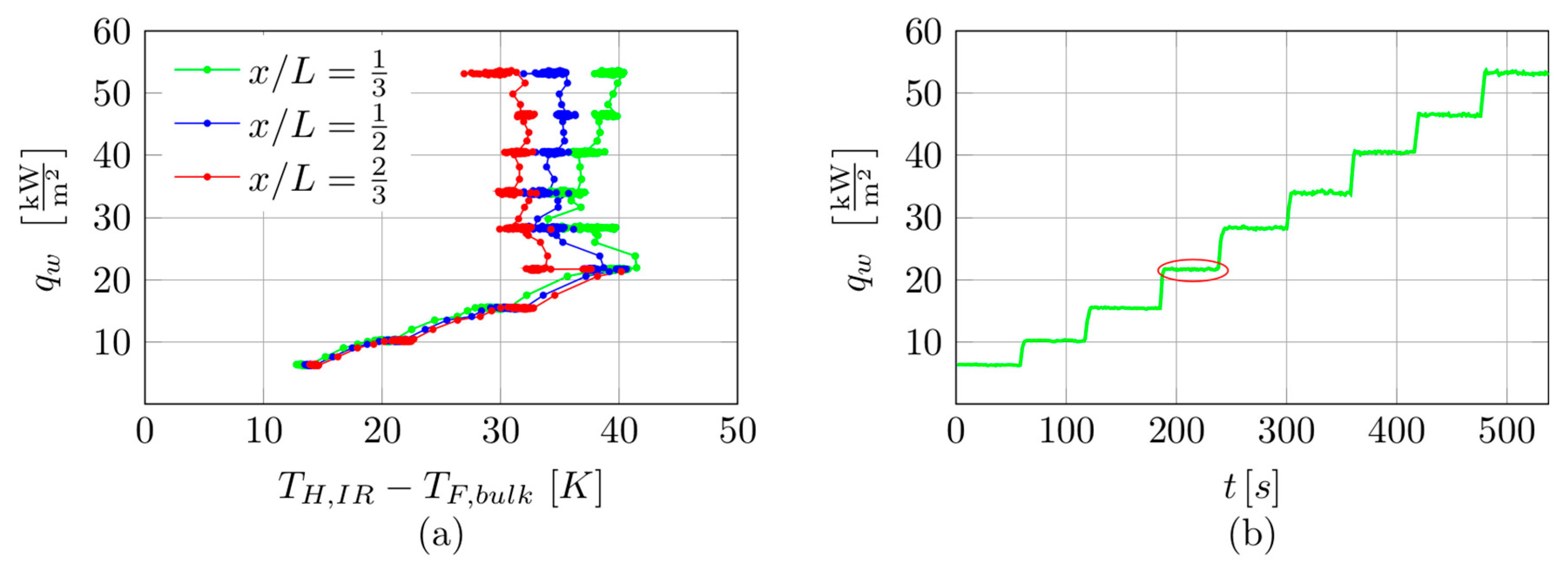
To present the main experimental data and results of the calculations, the example series with the test section comprising 17 minichannels was chosen. For a detailed illustration of the data and results regarding the subcooled boiling region, a narrower time interval of the entire experiment was selected. The data shown in
Figure 5 refer to this time interval of the experimental series during subcooled boiling, which is marked in
Figure 5b with a red ellipse.
Generally, the main experimental data collected during the experiment with 17 minichannels are illustrated in the following graphs:
Boiling curves, that is, heat flux versus temperature difference between the temperature of the heated wall and bulk fluid temperature for the selected point of the minichannel heated wall, as shown in
Figure 5a (based on the entire experimental data).
Heat flux density versus time—
Figure 5b (based on all experimental data).
Temperature measurement of the outer heated foil surface detected by infrared thermography illustrated as the distribution of temperatures versus coordinate x along the length of the minichannel and time—
Figure 6a (based on the selected experimental data at the subcooled boiling region).
Figure 5a presents examples of boiling curves obtained on the basis of data recorded during the entire experiment. These dependencies are plotted as functions of the imposed heat flux (density)
qw and the temperature difference between the heated wall
TH,IR (temperature measured on the outer heated wall surface by an infrared camera) and bulk fluid temperature
TF,bulk (assumed to change linearly along the minichannel length based on the measurements at the inlet and outlet by K-type thermocouples). Boiling curves were generated for the three selected points on the central axis of the wall of the minichannel. For this purpose, the following distances were chosen, that is,
x/L = 1/3,
x/L = 1/2, and
x/L = 2/3. The following comments can be drawn from the analysis of boiling curves. The subcooled liquid flowed into an asymmetrically heated minichannel. At the initial stage of heat flux increase, heat transfer from the heated wall to the fluid is governed by single-phase forced convection. In the vicinity of the heated wall surface, the liquid becomes superheated, whereas it remains subcooled in the core region of the flow. The appearance of spontaneous nucleation leads to a reduction in the temperature of the heated wall, called “nucleation hysteresis” [
8]. The reduction in heated surface temperature is initiated by the spontaneous formation of vapour bubbles, which act as internal heat sinks by absorbing significant amounts of thermal energy transferred to the fluid. A further increase in the heat flux leads to the development of nucleate boiling. The section of boiling curves concerned with the subcooled boiling region is of the main interest of this study.
During the course of the experiment, the imposed heat flux was increased stepwise, as illustrated in
Figure 5b. The selected time interval corresponding to the subcooled boiling region was considered in the analysis. During this time interval, the thermal and flow parameters were recorded for a constant heat flux every 1 s. The data were treated as captured under non-stationary conditions.
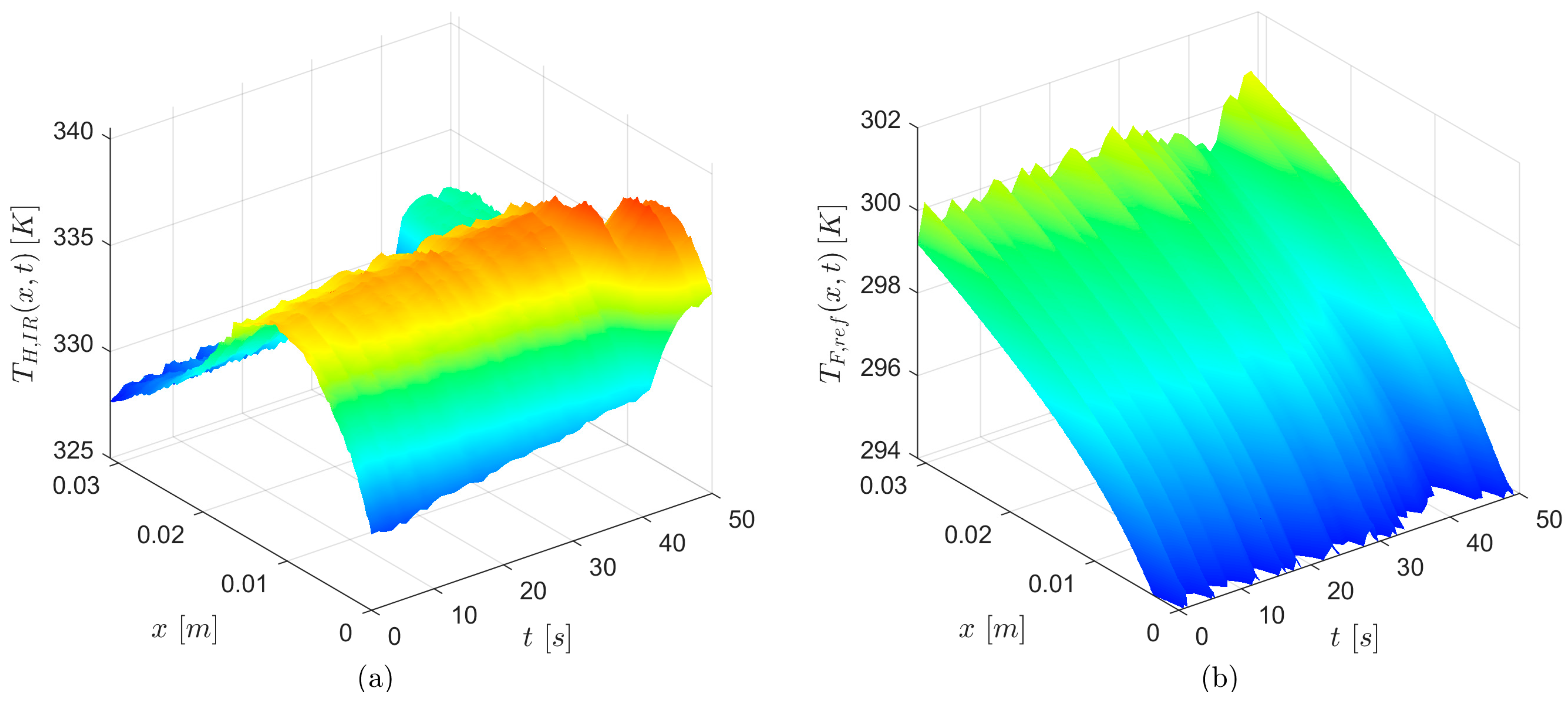
The distribution of temperatures versus coordinate
x along the length of the minichannel and time is illustrated in
Figure 6a. Variation in fluid temperature along the minichannel as a function of the axial coordinate
x, taken on the reference line in the fluid domain (taken from ADINA) and time, is also presented in
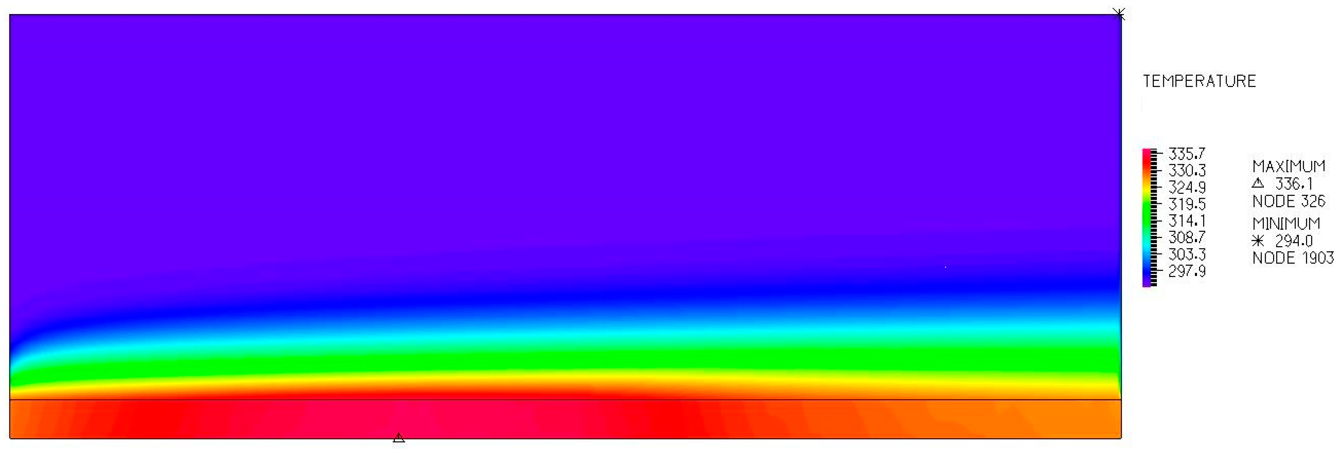
Figure 6b, based on the experiment chosen. Furthermore, the temperature distribution obtained from ADINA software at a selected time (
t = 25 s) is illustrated in
Figure 7.
According to
Figure 6a, it can be seen that the temperature of the heated wall captured for a specific average heat flux (time interval of 50 s) increases slightly with time, reaching its maximum in the middle of the minichannel length, while the maximum temperature difference was up to 10 K. Furthermore, as shown in
Figure 6b, the bulk fluid temperature increases with distance from the inlet, slightly differing in the time interval analysed.
The results of the numerical calculations performed at
qw = 21.3 kW/m
2 (time interval of 1 to 50 s of the selected experiment series with the test section comprising 17 minichannels) based on the experimental data, as shown in
Figure 5b and
Table 1, are illustrated in
Figure 8. The 3D graph presents local heat transfer coefficients and the coordinate
x along the length of the minichannel versus time
t, determined using two numerical methods based on the FEM as follows:
With the time-dependent Trefftz-type basis functions—
Figure 8b.
When analysing the results shown in
Figure 8, it can be observed that the heat transfer coefficient increases with the distance from the minichannel inlet at the selected time interval of 1–50 s, which is similar for both calculation methods. Furthermore, a significant increase in the coefficient values is observed during the last ten seconds near the minichannel outlet. The boiling initiation is often accompanied by an increase in the heat transfer coefficient [
8]. It can be underlined that the coefficient values determined from both methods do not differ significantly.
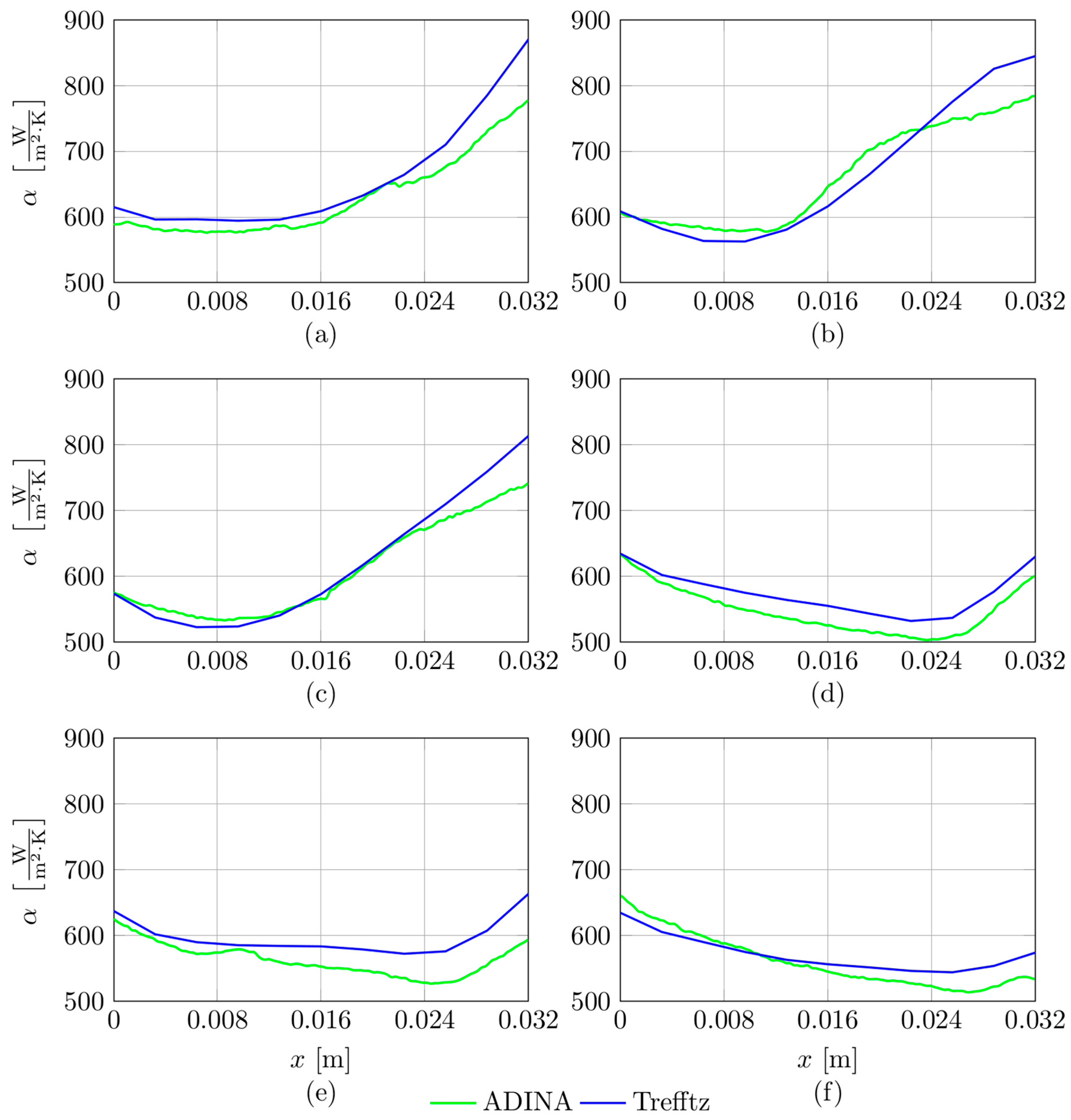
The results obtained from experiments in which the test section consisted of various numbers of minichannels (7, 15, 17, 19, 21, and 25) are shown in
Figure 9 as distributions of the heat transfer coefficient versus coordinate
x along the minichannel length at the average heat flux value of
qw = 22.2 kW/m
2. In each figure, curves based on the results from the application of two numerical methods based on the FEM are shown, i.e., based on the Trefftz functions (blue line) and performed in ADINA software (green line).
Based on the results shown in
Figure 9, the following observations were made:
If the test section comprises a smaller number of minichannels (7, 15, and 17), there was a significant increase in the coefficient values as a function of distance from the minichannel inlet, regardless of the calculation method considered (
Figure 9a–c).
For the number of 19 and 21 channels in the test section, the heat transfer coefficient first decreases with increasing distance from the inlet and near the outlet section (
Figure 9d,e), but this is approximately a 30% lower increase in coefficient values compared to that achieved for the test section comprising a smaller number of channels; heat transfer coefficients for the test section with 19 channels are slightly lower than for 21 channels, while their distributions are similar.
For the test section comprising the maximum number of minichannels (i.e., 25), the lowest values of the heat transfer coefficient were obtained in comparison with all analysed cases; the relationship displays a decreasing function with increasing distance from the inlet, almost for the entire minichannel length (except the region close to the outlet).
The heat transfer coefficient determined by applying the Trefftz function often achieved values higher than those obtained from the calculations by the ADINA programme. Moreover, it can be noticed that the highest discrepancies in the results are observed near the channel outlet. Detailed values of the differences in the values of the heat transfer coefficient calculated according to both methods are listed in
Table 3. These differences are the result of certain assumed simplifications in each of the numerical methods.
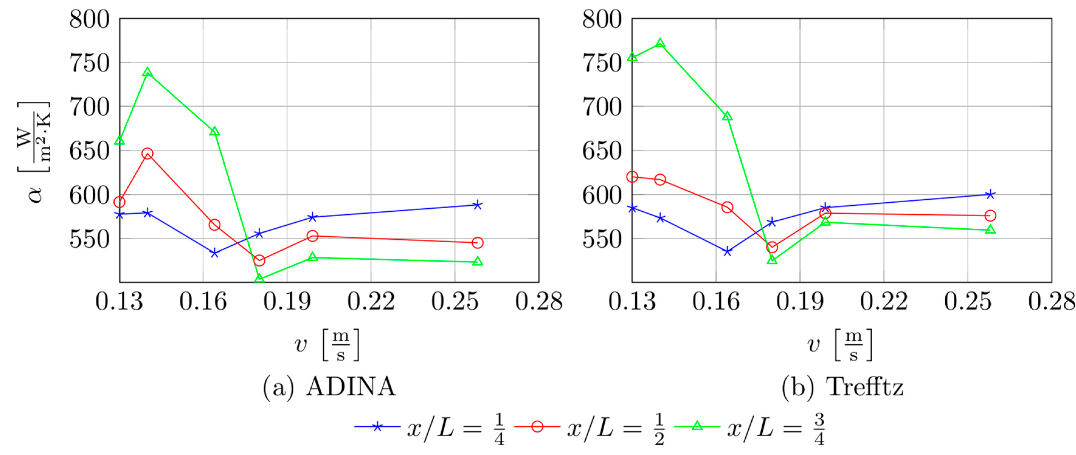
The use of a test section with a different number of channels has a direct impact on the flow velocity of the fluid in each channel, while the same total mass flow rate was established during each investigation. Increasing the number of channels is accompanied by a decrease in the flow velocity in individual channels of the group. The resulting heat transfer coefficients versus velocity at
qw,ave = 22.2 kW/m
2 for three selected distances from the minichannel inlet (¼, ½, and ¾ of channel length) and obtained from the calculation with ADINA software and with the use of Trefftz functions are presented in
Figure 10a,b, respectively. Calculations were carried out based on data recorded when the test sections comprised all numbers of minichannels, that is, 7, 15, 17, 19, 21, or 25 minichannels were investigated.
Generally, the following comments can be indicated with respect to the results shown in
Figure 10:
Higher values of the heat transfer coefficient are reached when the fluid flow velocity in a single channel is lower.
The heat transfer coefficient reached its lowest values at a flow velocity of 0.16 m/s within the minichannel.
The highest values of the heat transfer coefficient were recorded near the outlet section (for x/L = 0.75) and the lower flow velocities.
For a flow velocity in the range of 0.14–0.18 m/s, increasing the velocity causes a decrease in the heat transfer coefficient when taking into account the results gained for x/L = 0.5 and 0.75; analysing the results obtained for x/L = 0.25, a similar trend of decrease can be observed in the velocity range of 0.13–0.17 m/s.
For flow velocity in the range of 0.18–0.20 m/s, for larger distances from the channel inlet (x/L = 0.5 and 0.75), a slight increase in the heat transfer coefficient can be noticed; similarly, for a distance from the channel inlet corresponding to x/L = 0.25 and velocity values greater than 0.16 m/s, higher values of the heat transfer coefficient.
Above the flow velocity of 0.20 m/s, its further increase does not cause significant changes in the value of the heat transfer coefficient for x/L = 0.5 and x/L = 0.75.
When analysing the comments listed in points 4–6, a similar trend of all the analysed data was noted; moreover, it should be underlined that the development of the boiling process during flow occurs with increasing distance from the channel inlet.
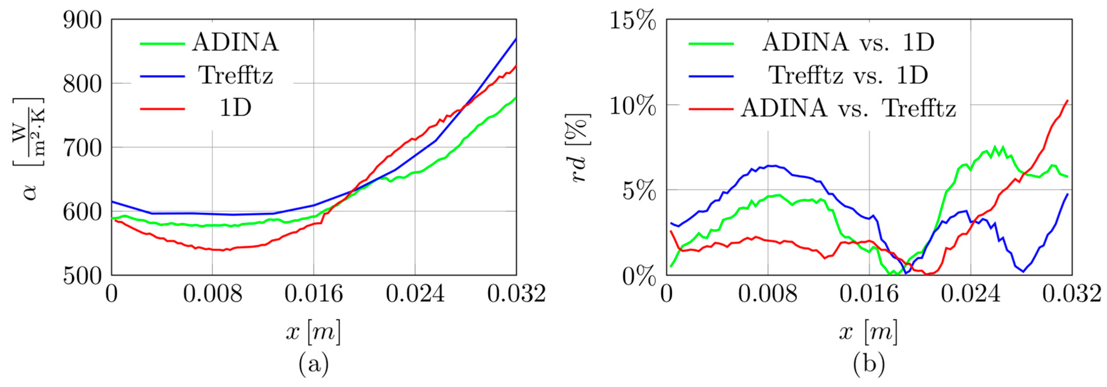
Calculations were carried out on experimental sample data collected for the test section comprising 17 minichannels and acquired at
qw = 21.3 kW/m
2. The results of the computations are shown in
Figure 11.
When analysing the curves shown in
Figure 11a, it is clear that a similar course was obtained for all dependencies. Furthermore, the highest differences between the heat transfer coefficient determined using the Trefftz method and according to ADINA software are reached at the minichannel outlet (up to 10%), as shown in
Figure 12b. The lowest differences between the coefficient values determined by both methods are obtained in the middle of the channel length.
An analogous formula was used to obtain relative differences between the heat transfer coefficients obtained by ADINA and the 1D method, Trefftz functions, and the 1D method. The results, in the form of the relative differences between the heat transfer coefficients obtained by each calculation method versus coordinate x along the minichannel length, are shown in
Figure 12b. The presented results were determined based on the data collected for the experiment with 17 minichannels. The lowest relative differences between the coefficients are observed near the middle of the channel length, while the highest values of the differences occur at
x/L = 1/3 distance from the inlet and near the outlet.
The relative differences between the heat transfer coefficient obtained by ADINA software and using FEM with Trefftz functions are presented in
Table 3 for the experiments with the test section comprising the number of minichannels
n. Furthermore, for
n = 17, relative differences between the heat transfer coefficients obtained by ADINA and the 1D method, the Trefftz function, and the 1D method were calculated, and the results have also been provided.
When analysing the data presented in
Table 3, it was noted that the results obtained by two methods (ADINA software and FEM using Trefftz functions) agree well with each other. The average relative difference reach a level less than 3% in more cases; only for
n = 7 and for
n = 17, they reach higher values (up to 10%). The maximum relative differences range from 11.6 to 26.5%, and the lowest values are achieved for a greater number of minichannels in the test section (19, 21, and 25). Furthermore, the relative differences between the results of both numerical calculations (ADINA software and FEM using Trefftz functions) and the results obtained from the 1D method reached the maximum values in the range of 21.2 to 25.7%, while the average relative differences values are between 2% and 9.9%. Furthermore, the average relative differences between the results obtained by ADINA software and by the 1D method are higher (approximately 10%) than the relative differences between the results obtained by using the FEM with Trefftz functions and by the 1D method (2%).
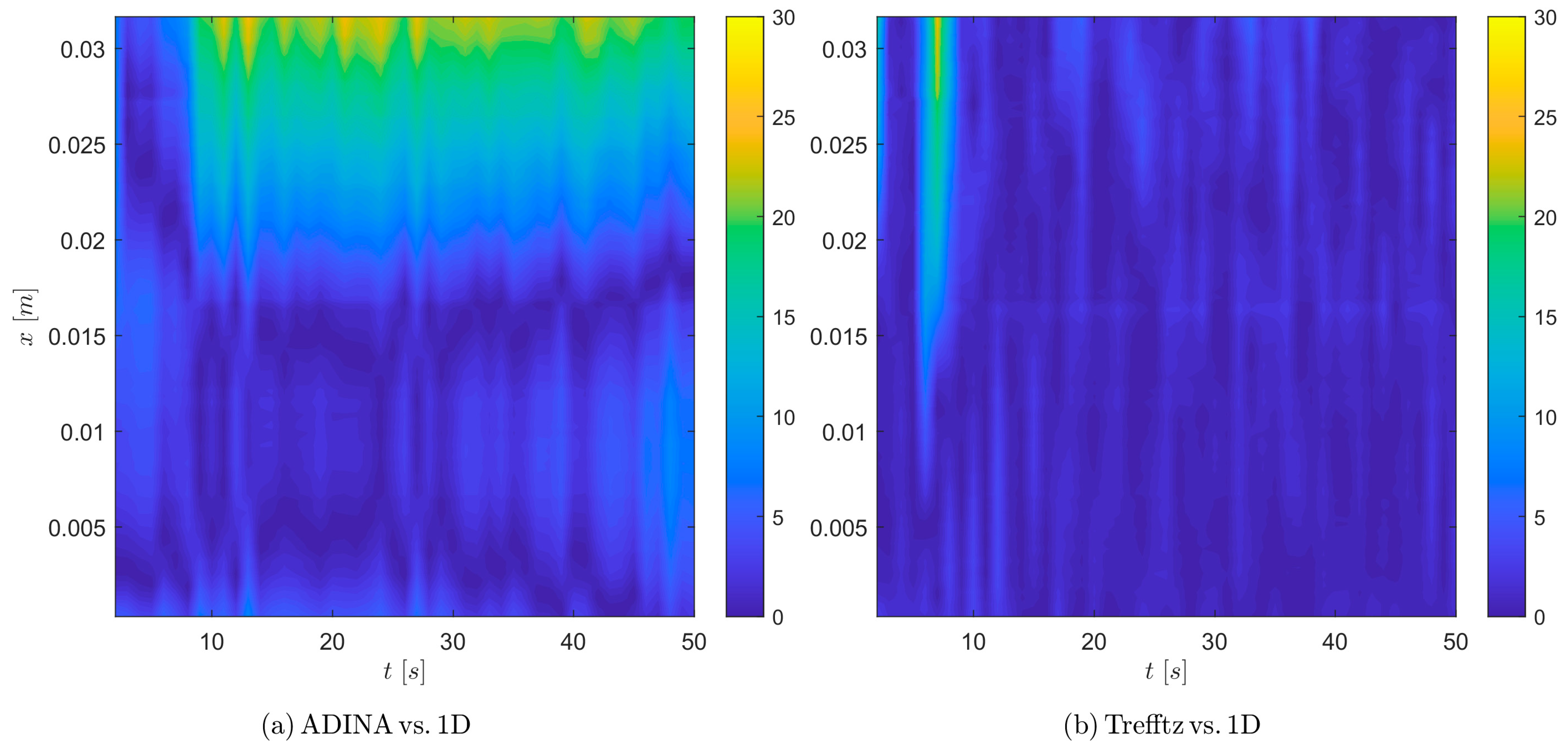
The distributions of the relative differences between the heat transfer coefficient obtained by two calculation methods in time
t and along the length of the minichannel are illustrated in
Figure 12. The graphs shown in
Figure 12 were created from data collected from the experiment with the test section comprising 17 minichannels at
qw = 21.3 kW/m
2. It can be seen that the largest relative differences are found near the outlet of the minichannel.
6. Conclusions
The primary aim of this study is to advance and spread knowledge about technologies and science for the sustainable development of energy. The results presented from numerical calculations are useful for designing minichannel heat exchangers. If such results are based on the data from the experiments, it helps to verify the correctness of the computations and will ensure that they are reliable. Furthermore, by verifying the numerical results with other methods, it can be ensured that the results are correct.
The main goal of the article was boiling heat transfer during fluid flow in 7, 15, 17, 19, 21, and 25 minichannels of 1 mm depth heated asymmetrically. The data of the experiments helped to realise the other objective, which is the mathematical modelling of the time-dependent heat transfer process during flow boiling in the subcooled boiling region. The main aim of the numerical calculations was to determine the heat transfer coefficient on the minichannel heated wall-flowing fluid contact surface. The coefficient was computed using the Robin boundary condition. To solve the heat transfer problem associated with time-dependent flow boiling, two numerical approaches based on the FEM were employed. One approach utilised Trefftz functions, while the other involved numerical simulations performed using the commercial software ADINA. Both numerical approaches used the same energy equations in the heated wall and in the flowing fluid. In the ADINA software, the mathematical model was additionally supplemented with the mass and momentum conservation equations. In calculations using the Trefftz function, the inverse problem of heat transfer was solved. The values of the heat transfer coefficient determined by both numerical methods were compared with the results obtained from a simplified one-dimensional model based on Newton’s law of cooling and experimental data.
Based on the results of the experiments and numerical calculations and analyses of the results, the following observations can be noted:
If the test section comprises a smaller number of minichannels, there is a significant increase in the heat transfer coefficient values, regardless of the calculation method considered.
Higher values of the heat transfer coefficient are reached when the fluid flow velocity in a single channel is lower.
Above the flow velocity of 0.20 m/s, its further increase does not cause major changes in the value of the heat transfer coefficient for all selected distances from the inlet.
The heat transfer coefficient determined with the application of the Trefftz function achieved values higher than those obtained from the calculations by the ADINA programme, but average differences between them are on the order of a few percent.
In the selected system of 17 minichannels, the average relative differences between the results obtained using the ADINA software and the 1D method do not exceed 10%, while the relative differences between the results obtained using FEM with Trefftz functions and the 1D method are about 2%.


