Abstract
The present study proposes two regression-based models for predicting the energy consumption of a four-axis prototype retail manipulator. These models are developed using experimental current and voltage measurements. The Total Energy Model (TEM) is a method of estimating energy per trajectory that utilizes global motion parameters. In contrast, the Power-to-Energy Model (PEM) is a technique that reconstructs energy from predicted instantaneous power. It has been demonstrated that both models demonstrate high levels of predictive accuracy, with mean absolute percentage error (MAPE) values ranging from 1 to 1.5%. These models are well-suited for implementation in hardware-constrained environments and for integration into digital twins.
1. Introduction
In an era of increasing automation and robotization of industrial processes, including autonomous systems, effective energy management is of paramount importance. For manipulators with multiple degrees of freedom, it is crucial not only to ensure precise control but also to optimize energy demand. Sustainable development and energy efficiency are among the primary directions for the robotics market in 2025, as highlighted by the International Federation of Robotics [1]. The average annual energy consumption of an industrial robot is approximately 22,000 kWh [2], which, given the rise of energy prices, translates into increasingly higher operational costs. The maintenance costs of a production line equipped with dozens of robots, at current energy prices, amount to hundreds of thousands of PLN annually. Reducing energy consumption by even a few percent yields tangible savings. In addition, it positively impacts the natural environment by contributing to the reduction of harmful emissions associated with electricity production.
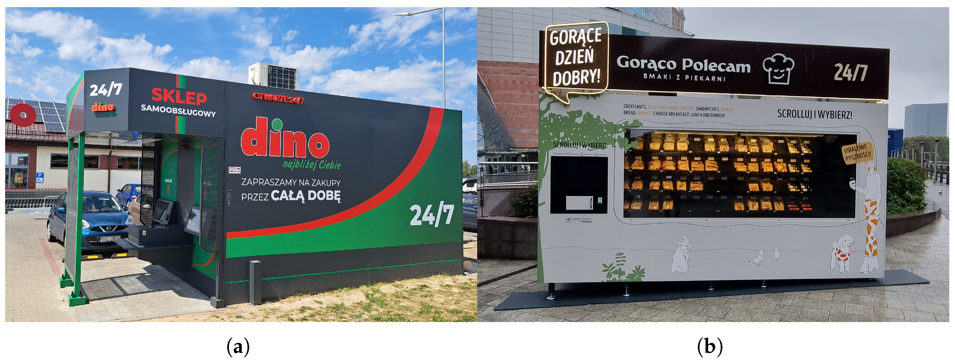
Automation plays a key role in improving efficiency and reducing operational costs across industrial and service sectors. In retail environments, robotic manipulators are increasingly adopted in automated stores, requiring precise control and energy-efficient operation due to their continuous 24/7 workload. Figure 1 illustrates the implementations of the automated stores developed by Hemitech.
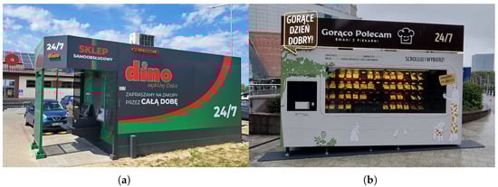
Figure 1.
Examples of automated stores developed and implemented by Hemitech: (a) Nexto Select, (b) Nexto Display. Reproduced with permission of Hemitech Sp. z o.o.
Digital twins are utilized in the design process of automated store systems. a recent publication [3] detailed the advancements in the digital twin of the Intelligent Automated Store warehouse. a significant component of the digital twin, from the perspective of energy efficiency, pertains to manipulator models, encompassing manipulator energy consumption models. These models serve as the foundation for energy consumption optimization.
Energy modeling of manipulators remains a significant challenge, particularly in the early phases of development where full dynamic parameter identification is often unavailable or impractical. Existing approaches frequently utilize non-linear modeling or advanced machine learning algorithms. However, these methods typically require extensive prior knowledge of system dynamics, larger datasets, or complex tuning. This study adopts multiple quadratic regression due to its low computational complexity, interpretability, and robustness for limited datasets. The method enables efficient feature selection and avoids overfitting while capturing key second-order interactions relevant to motion-induced energy variation.
The present publication details energy consumption modeling work base on logged data employing regression methodologies. The manipulator analyzed in this study is part of a next-generation automated store developed by Hemitech, where continuous operation and energy costs are critical design constraints.
1.1. Background
Various methods for optimizing the energy consumption of robots have been extensively documented in the research literature. These methods range from solutions implemented at the hardware level, such as the use of energy recovery systems [4], to those at the control level, including the optimization of dynamic motion parameters [5], motion trajectories [6], and the cyclogram of tasks performed [7]. A notable aspect of energy consumption optimization during the development stage involves the use of a manipulator model and the analysis performed within a simulation environment [8].
Although these approaches offer an effective means to improve energy performance, they often rely on detailed knowledge of the robot’s internal dynamics or access to specific hardware data. In many practical scenarios, especially during the design phase of novel manipulators, such information may be unavailable or incomplete.
To address these challenges, recent research highlights the increasing adoption of data-driven approaches, which enable energy consumption modeling and optimization without requiring detailed physical models. For instance, Pan et al. developed a regression-based model using XGBoost to predict energy consumption in welding robots with high accuracy and applied trajectory optimization via metaheuristic algorithms to achieve significant energy savings [9]. Similarly, Zhang and Yan proposed a machine learning method using a genetic algorithm to optimize energy usage in industrial robots by capturing non-linear dependencies between operational parameters and energy output [10]. These methods show particular promise for systems where access to internal parameters or complete physical modeling is impractical.
Against this backdrop, the development of an accurate model of energy consumption of manipulators, particularly for newly designed specialized systems, assumes a significant role in addressing the energy consumption optimization issue. This necessity motivates the present study, which focuses on the use of regression methods for preliminary modeling of the energy consumption of a prototype manipulator dedicated to automated product sales. By applying multiple quadratic regression, this work seeks to bridge the gap between model availability and predictive performance at the development stage.
1.2. Brief Literature Review
Regression models are statistical methods used to predict a modeled variable based on independent variables. Regression techniques are widely applied to model energy consumption in various sectors, such as construction, to assess the energy demand of buildings [11], or industry, to improve the energy efficiency of factories [12]. In logistics systems employing mobile robots, linear regression is used to monitor battery status depending on selected trajectories and operational conditions [13].
Within the field of robotics, regression methods have been widely used to predict energy consumption as a function of robot dynamics, trajectories, or load parameters. Initially, such models often took the form of simple linear regressions based on power measurements or dynamic equations [8]. However, recent studies indicate a growing preference for more expressive approaches that better reflect the non-nonlinearities inherent in robotic systems.
In response to these limitations, more advanced techniques, such as ensemble regressors, extreme gradient boosting (XGBoost), and neural networks have recently demonstrated superior performance in predicting robot energy consumption, capturing complex non-linear relationships between joint torques and energy demands. These methods offer a compelling alternative, especially in cases where only limited sensor data are available. In particular, in scenarios with restricted observability, simulated power data have proven useful as a proxy for dynamic model identification [14].
Furthermore, several studies emphasize the applicability of regression-based models to novel or prototype systems, where detailed CAD or mechanical models have not yet been validated. Approaches employing transfer learning [10], KAN-LSTM models [15], or polynomial regression combined with automated parameter tuning [16] demonstrate robust performance even in early-stage system design. These developments form the conceptual and methodological foundation for the present study.
Recently, chaos theory has demonstrated significant utility in forecasting energy consumption within nonlinear dynamical systems by uncovering deterministic structures in complex time series. Ramadevi and Bingi offered a comprehensive review of chaotic time-series forecasting techniques combined with machine learning, such as phase-space reconstruction, Lyapunov indicators, and hybrid neural networks (CNN, LSTM, RBF)—showing their superior performance across various energy-related tasks [17]. A particularly relevant example is the phase-space-based chaos model for building energy consumption in a shopping mall, where Lyapunov exponent analysis paired with neural network estimation significantly outperformed traditional statistical forecasting methods [18]. Extending beyond predictive modeling, chaos-inspired methods have also shown promise for decentralized energy management. Bucolo et al. demonstrated that chaotic networks can autonomously regulate energy flows without centralized control [19], indicating a promising avenue for efficient energy coordination in multi-robot systems.
1.3. Contribution and Paper Organization
We propose two complementary modeling approaches aimed at capturing the energy usage of a four-axis manipulator under varied operating conditions, using actual experimental data. Primary contributions include:
- Design and implementation of a high-resolution measurement system capable of capturing power consumption parameters at the axis level, including real-time current and voltage monitoring across all servo drives.
- Development of two complementary regression-based models for energy consumption prediction:
- −
- The Total Energy Model (TEM), which directly estimates energy usage based on trajectory-level parameters such as distance, duration, and velocity;
- −
- The Power-to-Energy Model (PEM), which predicts instantaneous power over time and derives energy consumption through numerical integration.
- Application of multiple quadratic regression with iterative feature selection, balancing accuracy with model transparency and computational efficiency, especially suited for systems with limited training data.
The publication is structured as follows: Section 2 presents the materials and methods, including a description of the external measurement setup, data processing, kinematic model and the conducted experiment. Section 3 details the proposed models and evaluation methods. Section 4 presents the experimental results and their discussion. Section 5 concludes the article and outlines future research directions.
2. Materials and Methods
The primary objective of this research was to develop and compare methods for modeling the energy consumption of a manipulator based on experimental measurement data. The measurement setup was designed to enable the acquisition of electrical parameters from the manipulator’s power supply system. The data processing was complemented by the kinematic model of the manipulator, implemented in a PLC controller and within a Python 3.11.3 environment as part of a custom developed package.
For each trajectory, the time series of the manipulator’s position, velocity, and acceleration were calculated and used as input data for the models. These models were developed to estimate the total energy consumption of the manipulator, which was calculated for training purposes using measured data from the experiment.
2.1. Test Stand Description
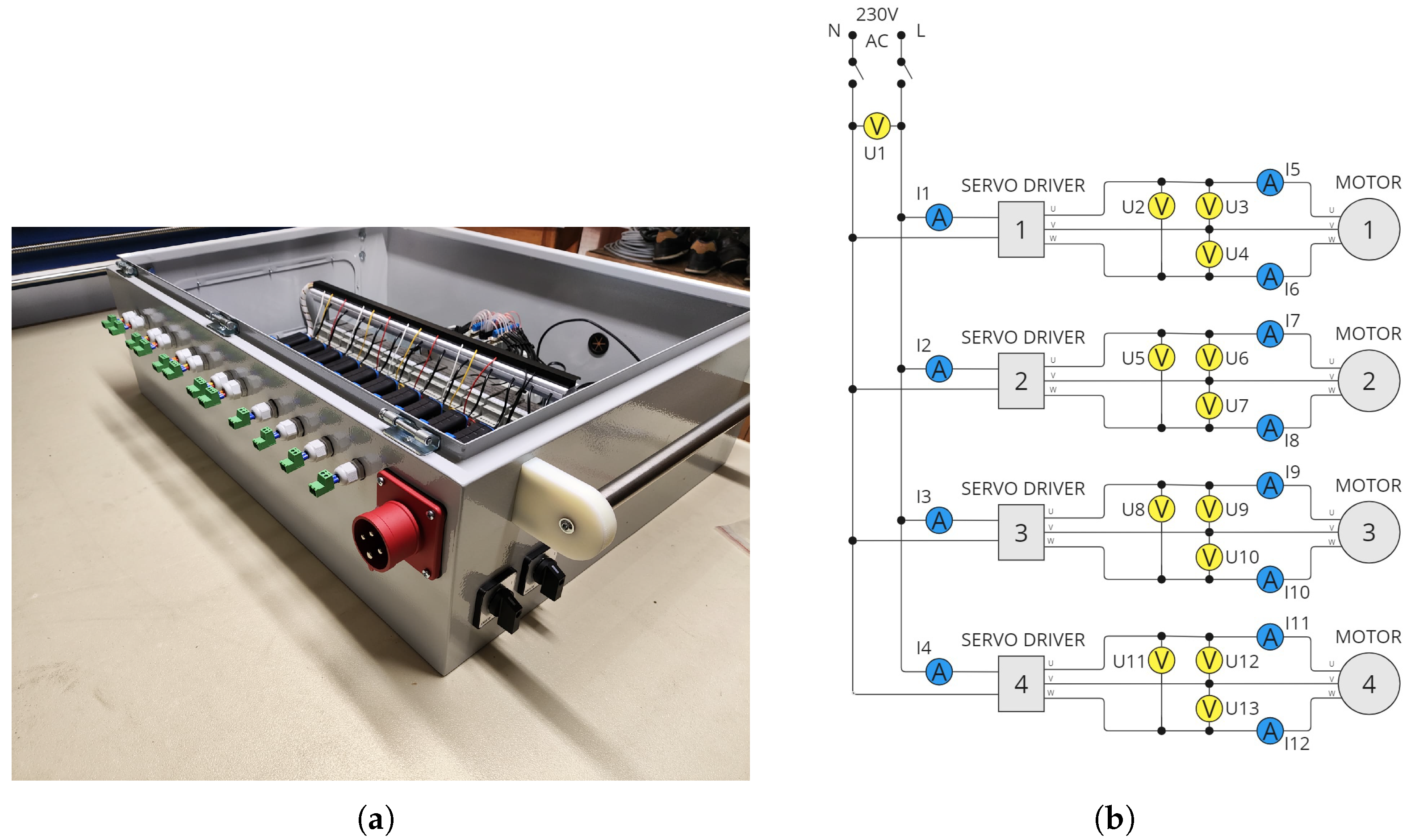
The experiments were conducted using a custom-designed research setup (Figure 2a), with its schematic illustrated in Figure 2b. The setup was configured to measure and log the current and voltage of AC/DC power supplied to four manipulators servo drives. The power supply parameters at both the input and output of the servo drivers were measured, and then used to calculate the instantaneous power for each manipulator axes. Based on the calculated instantaneous power, the total energy consumption of each manipulator drive can be estimated. The high time resolution of the measurements made it possible to calculate the energy consumption of each axis throughout the entire motion, including its distinct phases such as acceleration, constant velocity, and deceleration. Finally, the measurement system was integrated with the drive controllers housed within the control cabinet of the investigated manipulator.

Figure 2.
Test Stand: (a) physical implementation, (b) measurement diagram.
Hantek (Qingdao, Shandong, China) CC-65 current probes were selected, capable of measuring AC in the 40 Hz–2 kHz bandwidth in the range of 100 mA–10 A with ±2% accuracy. Voltage measurement was performed using a proprietary measurement system based on the Broadcom (San Jose, CA, USA) HCNR201 transoptor analog optocoupler with high linearity, designed for AC/DC voltage measurement in the range of ±600 V and up to 10 kHz bandwidth. All measurement signals were connected to a National Instruments (Austin, TX, USA) NI 9205 and a Chassis NI cDAQ-9172 measurement card. Thirteen supply voltage and twelve supply current measurements were logged for each waveform, according to the schematic shown in Figure 1b. In addition, a trigger signal from the servo drivers indicating the start of movement of each axis was logged. The sampling rate for all signals was set at 9500 Hz, with a 16-bit accuracy. For the purposes of this publication, the following sections focuses on the energy consumption associated with manipulator motors. It covers the measured values of U2–U13 for current voltages and I5–I12 for current intensities. All the methods presented in the following sections can be successfully used to predict the energy consumption of the power supply of servo controllers.
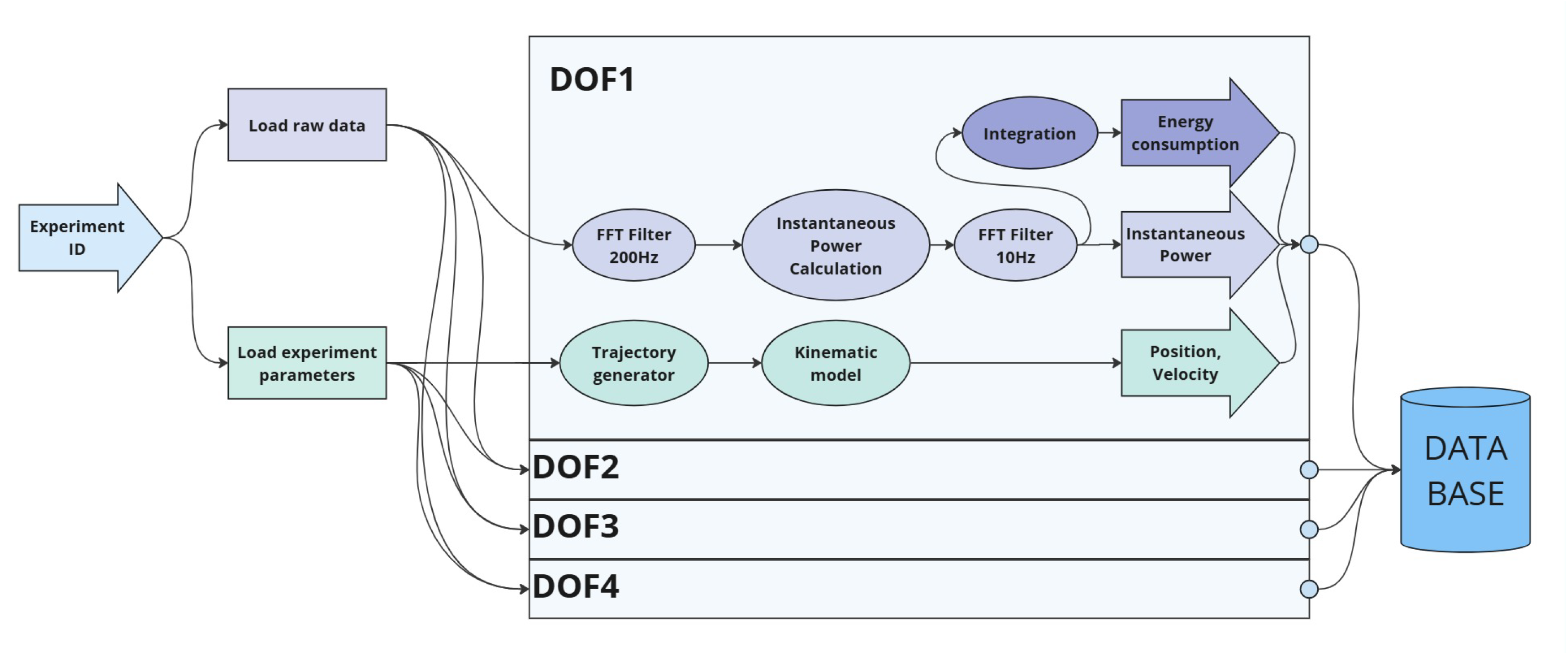
Data Preprocessing
In order to process the collected data, a special package was developed in the Python environment. This package loads and filters the measured data, converts the recorded power parameters into instantaneous power and energy consumption, and visualizes selected results. The process of calculating the energy consumption of the manipulator motors is shown in Figure 3.
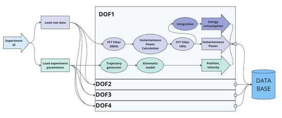
Figure 3.
Diagram of data preprocessing.
The first step after loading the data is low-pass filtering in the frequency domain using a Fast Fourier Transform (FFT). The scipy package [20] was used to perform the fast and inverse Fourier transform for the filter implementation. A cutoff frequency of 200 Hz was used for the measured parameters.
In the second step, the instantaneous power is calculated based on measurements of the motor supply voltage and current according to IEEE 1459-2010 [21]. For a three-phase motor, the instantaneous power is equal to the sum of the instantaneous powers in each phase. The measured phase-to-phase voltages were converted to phase voltages based on the vector method according to Equation (1).
where:
- —motor phase voltages,
- —motor phase-to-phase voltages,
- —motor phase currents.
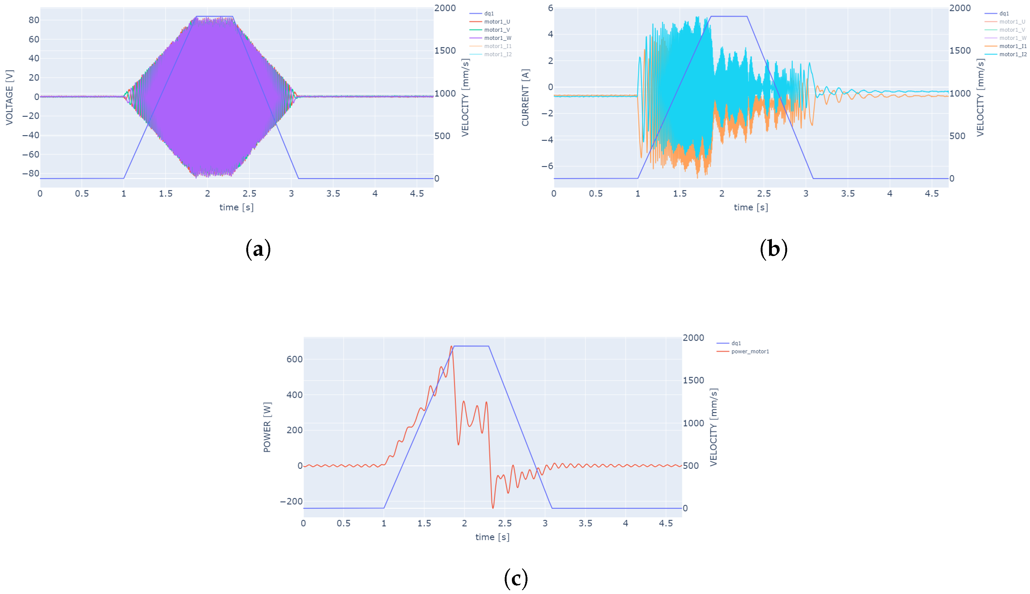
From the measurement of the current intensities of two phases, the currents of the third phase were calculated (2). The instantaneous power of the entire motor was calculated from Equation (3). A low-pass filter with a cut-off frequency of 10 Hz was applied to the instantaneous power waveform. Figure 4a,b show the phase voltage and current waveforms in the measured motor coil phases used to calculate the power. Figure 4c shows an example of the instantaneous power waveform based on actual measurement data for the DOF1 drive. The speed profile of the set motion is shown in blue on the graphs. Finally, the instantaneous power waveform is integrated over time according to Equation (4) to calculate the energy consumption of each drive.

Figure 4.
(a) measured phase voltage of the current in the motor coils, (b) measured current in the motor coils, (c) calculated instantaneous power.
2.2. Kinematic Modeling
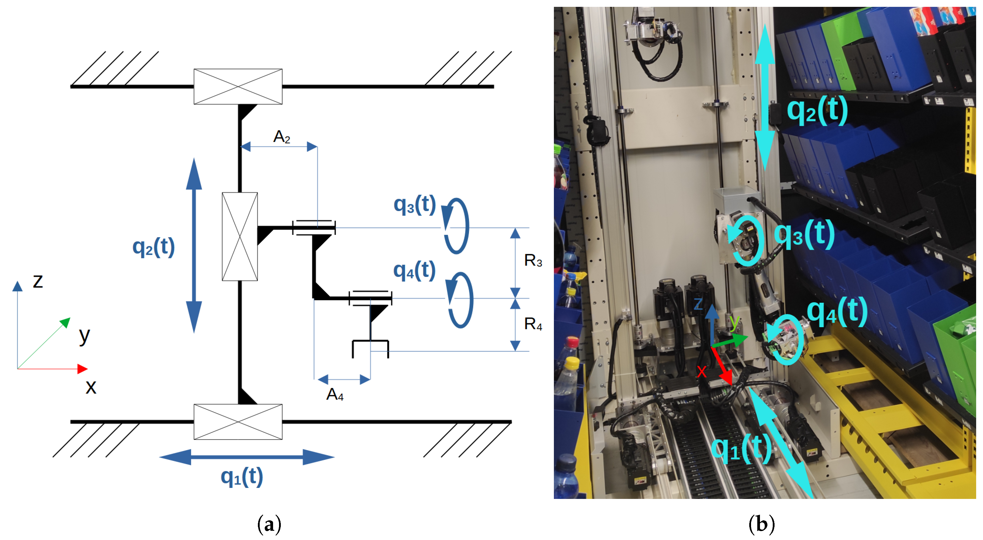
The experiment was performed on a prototype manipulator consisting of two positioning axes in the XZ plane—DOF1, DOF2 and an arm with two degrees of freedom (responsible for the manipulation task—DOF3, DOF4). The kinematic diagram and prototype of manipulator are shown in Figure 5. The manipulator uses DELTA-ECMA series AC servo drives from DELTA Electronics (Neihu District, Taipei, Taiwan) with 1500 W/750 W for the first two degrees of freedom and 400 W/100 W for the arm axis.

Figure 5.
Custom retail manipulator: (a) kinematic diagram, (b) real object. Reproduced with permission of Hemitech Sp. z o.o.
The manipulator’s kinematic model was developed using standard Denavit-Hartenberg (DH) notation [22], enabling both forward and inverse kinematics solutions. Forward kinematics computes the position and orientation of the end effector as a function of the joint positions and angles using homogeneous transformation matrices (5):
where each matrix follows the standard DH convention (6):
The DH parameters used for the manipulator design are summarized in Table 1. The complete forward kinematics is presented in a homogeneous transformation matrix (7). For inverse kinematics, analytical trigonometric solutions were derived (8)–(12), exploiting the relatively simple serial-parallel structure of the arm. The kinematic model was implemented both in a DELTA AX8 PLC (Motion CODESYS libraries) and in a custom Python package, allowing automated generation of trajectories with trapezoidal velocity profiles. This ensures full reproducibility of input motion profiles used for regression model training.
where: , , , , , —given position in cartesian coordinate, —element of the given orientation matrix.

Table 1.
Parametrs of Denvit-Hartenberg of Custom retail manipulator.
Accurate kinematic modeling is critical for generating reliable dynamic parameters influencing energy consumption. Recent studies [23,24] emphasize the importance of integrating precise kinematics into energy consumption models.
2.3. Experiments Design
In the experiment, manipulator movements were performed by controlling each axis individually according to a previously prepared experimental design. The experimental design was based on Halton’s quasi-random sampling method [25]. This method was chosen because of its deterministic nature and the uniform distribution of points in all dimensions of the sampling space, while ensuring that the points generated were not too close to each other.
For each axis of the manipulator, five motion parameters related to start and end positions and dynamic parameters related to accelerations and maximum velocity were defined to prepare the experiment. An additional parameter was the external load on the manipulator, determined by the mass of the manipulation object. The experimental parameters were selected based on the actual operating conditions of the prototype manipulator. The external loads were used to simulate the cross-section of the products that are handled by the manipulator. Containers specifically designed for this purpose were utilized; these containers are shown in Figure 5b (blue, green, and black containers). The selected dynamic parameters and the mass of the manipulated object are the main factors impacting the energy consumption [26].
Each axis motion parameter could take any value within a predefined range. The load parameter took one of four predefined values. The maximum load was equal to the predicted mass of the maximum manipulated object. The parameter space of the experiment is shown in Table 2. All start and end positions and their combinations within the defined ranges of motion fell within the manipulator’s working space. The ranges of the defined maximum velocities and accelerations were within the dynamic limits of the individual manipulator drives. The experiment included a total of 1591 measurement runs, with measurement times ranging from 3 s to 25 s.
Table 2.
Experiment parameters space.
3. Mathematical Modeling of the System
The primary objective of this study was to develop a predictive model for the energy consumption of a manipulator based on the collected data. For this purpose, two different modeling approaches were evaluated:
- Direct modeling of the total energy consumption,
- Indirect calculation of energy consumption based on instantaneous power modeling.
In both cases, the energy consumption model of the manipulator consists of sub-models related to the energy consumption of each axis, based on regression models.
3.1. Regression Model
The foundation of all sub-models is rooted in the principles of multiple quadratic regression methods. These methodologies empower the modeling of a linear combination of multiple independent variables and quadratic terms of them. The general form of the model is expressed as follows (13):
where:
- y—dependent variable (output),
- —linear terms,
- —interaction terms for ,
- —quadratic terms,
- —intercept,
- —coefficients for linear terms,
- —coefficients for interaction terms between different predictors,
- —coefficients for quadratic terms.
From a physical perspective, the use of multiple quadratic regression is further justified by the analytical structure of robot dynamics equations. As illustrated in classical formulations (e.g., using Lagrangian or Newton-Euler approaches), joint torques, and consequently energy consumption, are expressed as nonlinear functions of joint positions, velocities, and accelerations [27]. These equations typically include quadratic terms (e.g., velocity), interaction terms, and mixed products involving kinematic parameters and trigonometric functions. Although regression model does not explicitly reconstruct these physical quantities, it leverages the same functional relationships by learning them directly from data. It is important to note that trigonometric dependencies are not directly encoded in the regression terms. This simplification was deliberately adopted to reduce model complexity. As energy consumption is closely related to mechanical power (), the regression structure used in this study remains physically meaningful while avoiding overfitting or reliance on unavailable dynamic parameters.
In the context of energy consumption modeling, the independent variables corresponded to the dynamic parameters of movement for each axis of the manipulator, the path distance, the duration of movement, and the external load. The dependent variable of interest was defined as the energy consumption of each axis or the averaged instantaneous power. Prior to the training phase, a series of standardization procedures were implemented to ensure the integrity and comparability of the data. The training of the models was an iterative process. Initially, a model incorporating all independent variables and their combinations was trained. Subsequently, the list of independent variables was narrowed down based on an assessment of their statistical significance within the model and the value of the regression coefficients. For the subsequent step, only those variables were selected whose p-value was below 0.05 and the absolute value of the coefficient was greater than 0.01. The new model was then trained on the narrowed list of independent variables, and this procedure was repeated until the effect of all independent variables was statistically significant and the regression coefficients were greater than 0.01.
The regression models were prepared using the statsmodels package [28]. The data standardization was based on the StandardScaler class of the sklearn package [29].
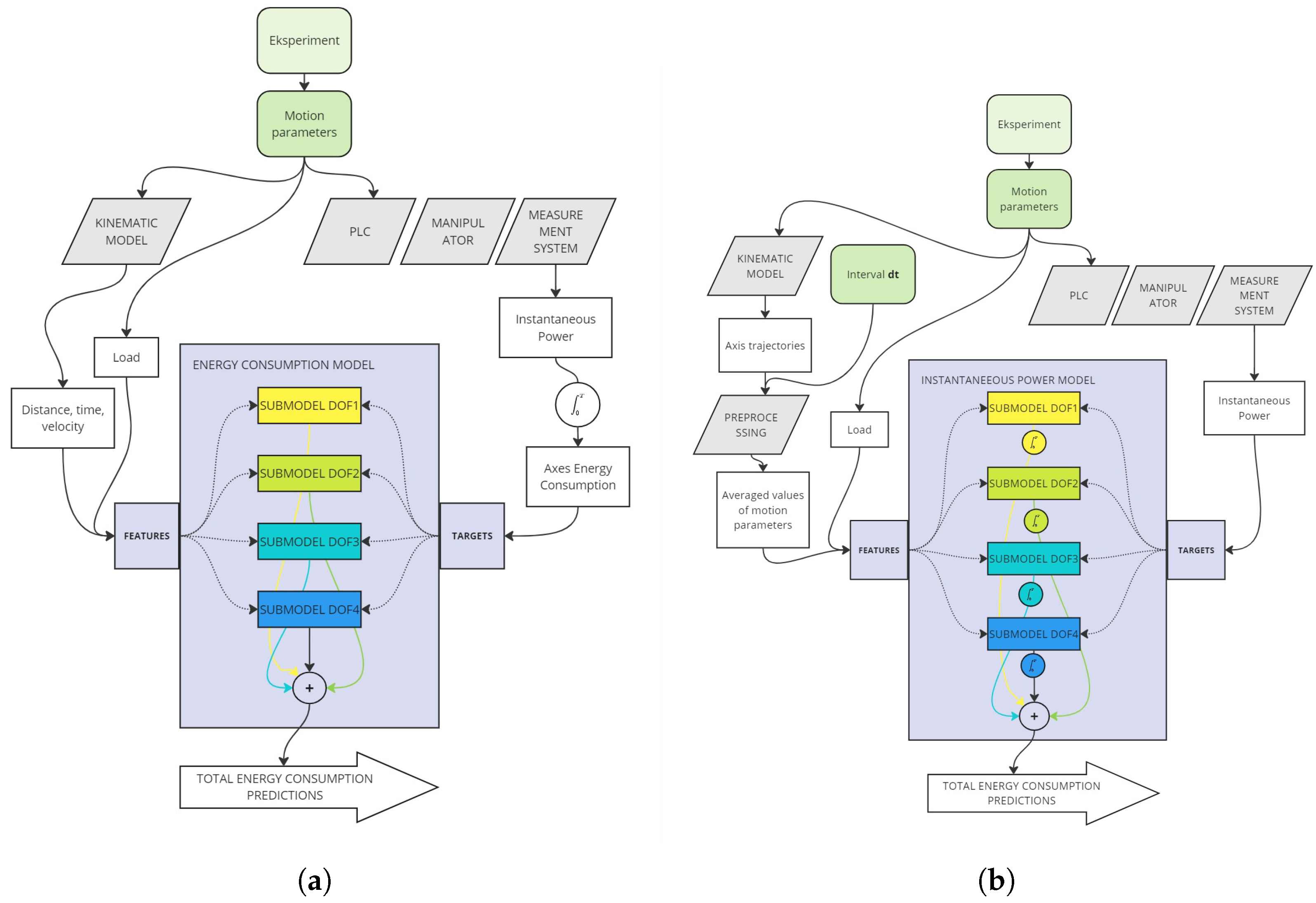
3.2. Total Energy Model
The first approach involves direct modeling of the total energy consumption of each axis during movement (Total Energy Model—TEM). The schematic representation of the TEM model is depicted in Figure 6a. The manipulator energy consumption model comprises sub-models for each axis. The input data utilized for the models encompass the total path distance of each axis, the duration of movement, the maximum achieved velocity, and the average velocity of each axis during movement. Additionally, the external load was involved. The modeled value was the energy consumption of each axis of the manipulator, calculated on the basis of power measurements collected during the experiment.
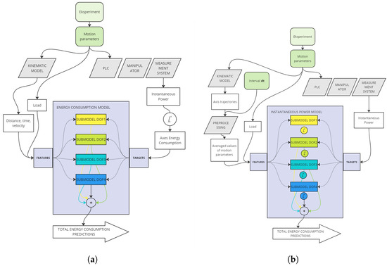
Figure 6.
(a) Diagram of Total Energy Model, (b) diagram of Power to Energy Model.
3.3. Power to Energy Model
The second model that was developed employed an indirect approach to predict the energy consumption of the manipulator. The modeled values were the instantaneous powers of each axis of the manipulator. A schematic representation of the prepared model is depicted in Figure 6b. The input data comprised the mean instantaneous values of position, velocity, and acceleration, derived from the trajectory that was calculated using the manipulator kinematic model. To ensure a comprehensive evaluation, the input data were augmented at each time instance with information regarding the external load. The modeled values, representing the instantaneous powers at different temporal points, were derived from the power measurements obtained during the experimental procedure. In order to calculate the energy consumption during the movement of each drive, it was necessary to predict the instantaneous power waveform for the entire movement. Integration over time of the instantaneous power values, according to Equation (13), makes it possible to determine the energy consumption. The energy consumption of the drives is summed to calculate the total energy consumption of the manipulator.
3.4. Model Evaluation
The accuracy of the developed models was assessed by means of a cross-validation method, which was used to verify the generalization of the models for different learning and testing data sets. One of the most commonly used methods, called k-fold cross-validation, was employed. This method involves dividing the dataset into k equal subsets. The k − 1 subsets are used to train the model, while the remaining subset is used for testing. The process of training and testing is repeated k times. The final model score is the average value from all k tests. The cross-validation was implemented based on the KFold class of the sklearn package. The following metrics were selected to evaluate the accuracy of the models on the test data: mean absolute percentage error () and root mean square error (). To assess the accuracy of the model fit to the training data, the adjusted measure of fit of polynomial models (adjusted coefficient of determination) and the Akaike information criterion () taking into account the model’s fit to the data, as well as its complexity expressed in the number of parameters, were used. The values of the and metrics are calculated within the statsmodel package during the regression model fitting process. Other metrics are calculated according to the Formulas (14) and (15).
where:
- y—real values,
- —predicted value,
- n—number of samples.
To complement the evaluation with a measure of statistical reliability, a 95% confidence interval was additionally computed for the mean values of and across the 10 cross-validation folds. The confidence interval was calculated assuming a Student’s t-distribution according to the standard formula:
where:
- —sample mean value,
- s—sample standard deviation,
- n—number of folds,
- —critical value of the t-distribution for confidence level and degree of freedom .
This provides an interval in which the true expected value of the metric is likely to lie with 95% confidence, allowing a more robust comparison of model performance.
4. Results and Discussion
The energy consumption models were prepared for the two proposed methods based on the collected measurement data and the kinematics model.
4.1. Total Energy Model Results
A critical element in the development of an accurate energy consumption model is the selection of appropriate input data. To identify the set of input parameters that optimally model energy consumption, a comparison of model accuracy was conducted. The average value of the metric calculated for a k-fold cross-check (k = 10) performed on all 1591 measurement runs was selected for comparison. The following sets of input parameters were compared:
- move-param—the data set contains 25 variables, including path distances, absolute values of path distances (not taking into account the direction of movement), accelerations, maximum velocity achieved, deceleration of each axis, and the value of external load,
- time—the data set contains 13 variables, including the durations of the acceleration, constant velocity motion and deceleration phases of each axis, and the value of the external load,
- dist-time—the data set contains 9 variables, including path distances and duration of each move phases of each axis, and the value of the external load,
- dist-abs-time—similarly to dist-time including absolute values of path distances,
- velocity-time—the data set contains 9 variables, including duration of movement and mean velocity values of each axis, and the value of the external load,
- dist-velocity-time—the data set contains 13 variables based on velocity-time extended by path distances of each axis,
- dist-abs-velocity-time—the data set contains 13 variables based on velocity-time extended by absolute values of path distances of each axis,
- all—the data set contains 29 variables, including a combination of all the above parameters except absolute values of path distances of each axis.
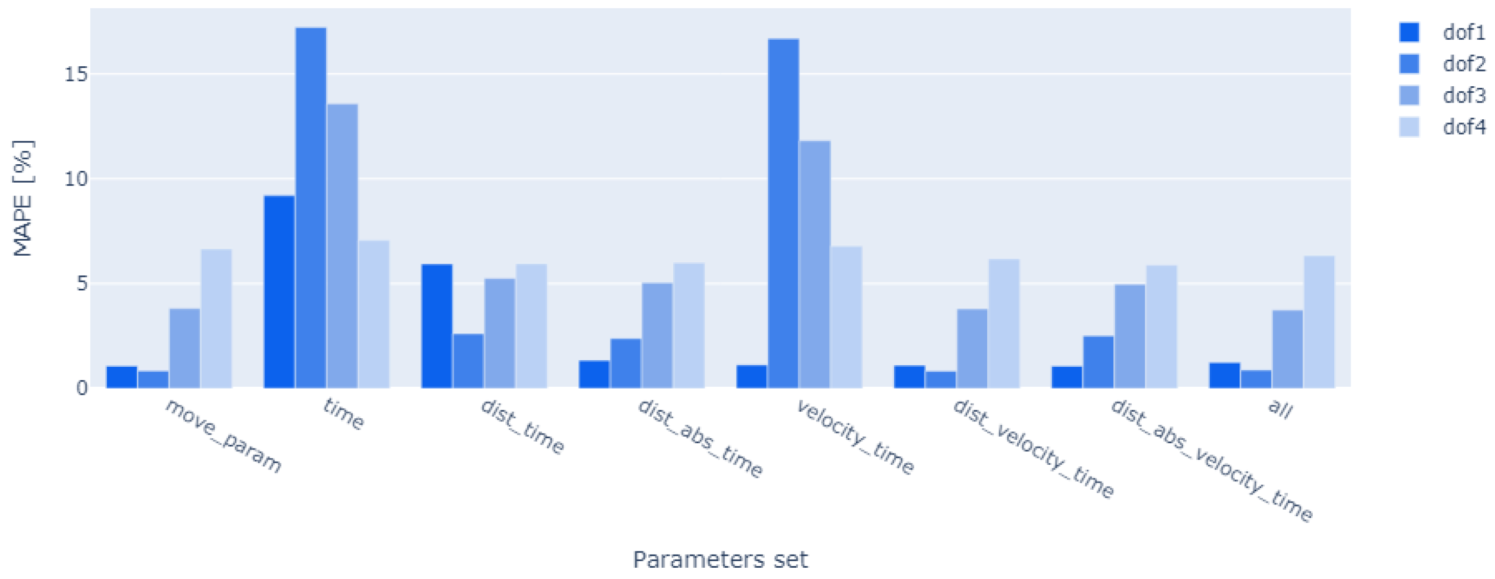
Figure 7 presents a comparative analysis of the mean absolute percentage error () values for a variety of input parameter datasets across the submodels.
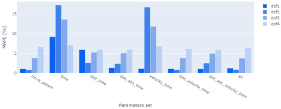
Figure 7.
Comparison of TEM models based on set of input parameters.
For DOF1, including velocity information in the input parameters allows for significant improvements in model accuracy. Accuracy for DOF2 and DOF3 axes is affected by information about the path distance, with information about the direction of motion improving the results. Accuracies for DOF4 models are not influenced noticeably by the selected input parameters. The best results of the submodels were obtained for the dist-velocity-time data set. Detailed metrics for the selected dataset are shown in Table 3. Further analysis reveals a very good fit of the first three axis models to the data ( parameters). Comparing the and averages, it can be seen that the overall model accuracy is mainly influenced by the first three axis models, which is consistent with the actual size of the drives used in the manipulator.
Table 3.
Mean metrics for TEM (dist-velocity-time) cross validation test.
For the set of dist-velocity-time parameters, the total energy consumption of the manipulator was also cross-validated by summing the values of all axes.
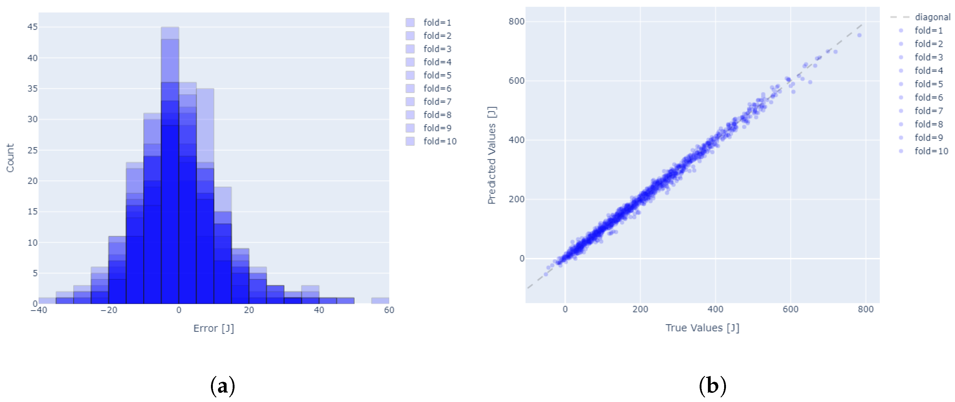
The statistics of the analyzed TEM model are presented in Table 4. The prepared model for the selected parameter set achieves average values of 1.3%, indicating high accuracy. Regardless of the data selected for training, the values of the standard deviation as well as the ranges of the minimum and maximum errors indicate a high repeatability of the models. The distribution of the residuals (Figure 8a) is very close to normal. The prediction results for the entire range of modeled values are close to the actual values (Figure 8b), indicating high efficiency of the model. The colors used in plots (a) and (b) correspond to individual folds employed in 10-fold cross-validation. In plot (a), a histogram of prediction errors is presented, where each shade of blue represents data from a different fold, enabling assessment of the error distribution across subsets of the dataset. Overlapping colors indicate how similar (or different) the error distributions are between folds. In plot (b), the color of each point denotes the fold from which the observation originates, allowing for evaluation of the model’s prediction consistency across folds. The dashed gray line represents perfect agreement between predicted and true values—the closer the points lie to this line, the more accurate the model’s predictions.
Table 4.
Statistics for MAPE and RMSE of TEM.

Figure 8.
(a) Residual histogram, (b) True vs. Predicted values for 10 fold cross validation test for TEM.
In addition confidence intervals for both and , calculated based on a Student’s t-distribution (16). These relatively narrow intervals further confirm the stability and reliability of the regression model across folds. The small margin of error around the mean values indicates that the predictive performance observed is consistent and not significantly influenced by the particular choice of training and testing subsets. This strengthens the evidence that the model generalizes well to unseen data within the considered parameter space.
4.2. Power to Energy Model Results
The PEM model is an indirect approach to modeling energy consumption. First, predictions are made of instantaneous power at the time of movement, and then energy consumption is calculated based on them. The input parameters for the developed models are the instantaneous values of position, speed, and acceleration, as well as the value of the load. The quality of the obtained model is greatly influenced by the time interval that describes the input parameters. Reducing the time interval enhances the temporal resolution of the instantaneous power prediction. A similar analysis to that conducted for the TEM model was performed, examining the impact of input data on the accuracy of the model. This analysis utilized the mean absolute percentage error () metric, calculated for the 10-fold cross-validation for all 1591 measurement runs. The following input data sets were compared:
- pos-vel-acc—the data set contains 13 variables, including the instantaneous values of position, velocity, and acceleration for each axis, as well as the value of the external load,
- pos-velabs-acc—the data set contains 13 variables, including the instantaneous values of position, absolute velocity, and acceleration for each axis, as well as the value of the external load,
- pos-vel-velabs—the data set contains 13 variables, including the instantaneous values of position, velocity and absolute velocity for each axis, as well as the value of the external load,
- vel-velabs-acc—the data set contains 13 variables, including the instantaneous values of velocity, absolute velocity and acceleration for each axis, as well as the value of the external load,
- pos-vel-velabs-acc—the data set contains 17 variables, including a combination of all the above parameters.
Furthermore, the impact of the width of the time intervals was evaluated for each input dataset. The analysis encompassed time intervals of 0.4 s (14,765 samples), 0.2 s (25,579 samples), 0.1 s (47,155 samples), and 0.05 s (90,302 samples).The results of this comparison are illustrated in Figure 9. To improve the clarity of the findings, the mean absolute percentage error () value was calculated for all axes for each input data set and time interval.
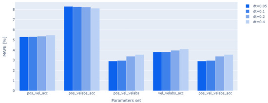
Figure 9.
Comparison of PEM models based on set of input parameters and interval time.
The incorporation of redundant data, in the form of instantaneous velocity waveforms and their absolute values, has been demonstrated to remarkably enhance the model’s prediction accuracy. In contrast, the impact of the instantaneous value of acceleration has been found to be negligible. The accuracy of the prediction of energy consumption is observed to improve with the time resolution at which the prediction of instantaneous power waveforms is conducted. The parameter dt being inversely proportional to the prediction accuracy, i.e., smaller values of dt result in more precise predictions. The differences in accuracy are negligible when time intervals of dt = 0.05 s and dt = 0.1 s are employed. For further analysis, a set of pos-vel-velabs parameters was selected for the interval dt = 0.1 s, for which detailed metrics are shown in Table 5.
Table 5.
Mean metrics for PEM (pos-vel-velabs, dt = 0.1) cross validation test.
In the case of the analyzed PEM model, the predictive power and fit quality are optimal for the first three degrees of freedom (DOF1–DOF3). However, the metrics of the fourth axis, = 0.475, indicate a suboptimal fit of the model to the data. A further analysis of the root mean square error () values reveals that the predictions of the first two axes primarily determine the overall accuracy of the manipulator’s results.
A comprehensive evaluation of model accuracy is shown in Table 6. The average value of MAPE prediction errors for the entire manipulator was 1.52%, indicating high accuracy of the models. The values of the standard deviation as well as the ranges of the minimum and maximum errors indicate high repeatability of the models regardless of the data selected for learning. The distribution of the residuals (Figure 10a) as well as the plot of actual to predicted values (Figure 10b) show high prediction accuracy. The manner in which the data is presented is analogous to the residual distribution and true values of the TEM model depicted in Figure 8. The confidence intervals, although slightly wider than those obtained for the TEM model, still demonstrate a high level of consistency and robustness of the PEM approach across the folds. The magnitude of the confidence bounds reflects both the increased temporal resolution and the complexity of modeling instantaneous power over time. Despite this, the predictive accuracy remains tightly bounded, confirming that the PEM model reliably reconstructs energy profiles with minimal variability and strong generalization across varied motion and load conditions.
Table 6.
Statistics for MAPE and RMSE of PEM.
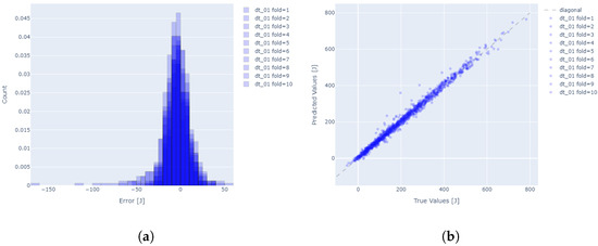
Figure 10.
(a) Residual histogram, (b) True vs. Predicted values for 10 fold cross validation test for PEM.
4.3. Discussion
Both proposed models achieved high prediction accuracy, with a mean absolute percentage error (MAPE) ranging from 1% to 1.5%. The highest submodel errors occurred for DOF4, primarily due to mechanical imperfections and low drive power resulting in increased vibrations during high-dynamic motions. However, due to the low energy demand of this axis, its influence on total error remains negligible. In the PEM model, reducing the input time interval improves accuracy, with optimal results at 0.1 s. Further reduction degrades performance due to high-frequency measurement noise that affects polynomial regression fitting. This behavior reflects the limitations imposed by the filtering process and sampling resolution. The TEM model provides direct energy estimation from global trajectory descriptors and requires fewer parameters, enabling fast inference suitable for real-time applications. In contrast, the PEM model, while more computationally intensive, reconstructs energy from predicted power profiles and offers higher temporal resolution, which is useful for simulation and digital twin environments.
The proposed method, based on multiple quadratic regression, achieved prediction accuracy comparable to advanced machine learning techniques. Pan et al. (2025) reported a MAPE of 1.86% using an XGBoost-based model for welding robots [9]. Jiang et al. (2025) applied a hybrid LSTM-CNN architecture that achieves MAPE values below 1.7% in certain configurations [30]. Chang et al. (2024) obtained MRE of 1.64% with a BN-LSTM architecture and improved it to 1.18% using KAN-LSTM [15]. These methods typically require extensive training datasets and high computational resources. In contrast, the presented regression models are lightweight, fully interpretable, and suitable for deployment in embedded systems or early-stage designs with limited data. By including interaction and quadratic terms, the models capture essential non-linearities while remaining analytically tractable. It should be emphasized that the motion complexity of the prototype retail manipulator investigated here is substantially lower than that of welding or general-purpose industrial robots. Its kinematic structure is strictly tailored to its operational tasks, which allows for the use of simpler energy consumption models without compromising predictive accuracy.
5. Conclusions
The study demonstrates that multiple quadratic regression, combined with systematic feature selection and integration of accurate kinematic modeling, can provide highly accurate energy consumption predictions for a retail prototype manipulator. This suggests that even simple, transparent models may be sufficient for early-stage development, rapid prototyping, or integration into digital twins, without the complexity of non-linear or full physical dynamic models. Compared to alternative modeling techniques in the literature (non-linear regression, neural networks, physics-informed simulation), our approach offers several advantages: ease of implementation, interpretability, full reproducibility, and suitability for limited datasets—a common situation for prototype devices. The high prediction accuracy observed demonstrates that much of the manipulator’s energy demand can be effectively explained by trajectory-level kinematic variables and external load, without requiring full dynamic parameter estimation.
Future research will explore the integration of non-linear machine learning techniques (e.g., SVR, random forests, deep neural networks) to capture more subtle non-linear behaviors observed especially under high dynamics or larger payloads. Moreover, applying the proposed methodology to a variety of manipulator architectures will allow testing generalization and potential limitations of the regression-based approach.
Author Contributions
Conceptualization, P.K., K.L. and P.P.; methodology, P.K., K.L. and P.P.; software, P.K.; validation, P.K.; formal analysis, P.K.; investigation, P.K.; resources, P.K.; data curation, P.K.; writing—original draft preparation, P.K.; writing—review and editing, P.P. and K.L.; visualization, P.K.; supervision, P.P. and K.L.; project administration, P.K.; funding acquisition, P.K., P.P. and K.L. All authors have read and agreed to the published version of the manuscript.
Funding
The research presented in the paper was conducted and funded by the Ministry of Education and Science of Poland: RJO15/SDW/006-19 as part of the first author’s PhD thesis. The custom retail manipulator was developed by Hemitech within the Intelligent Cell Cluster of the Automated Store Warehouse (iZMS) project (POIR.01.01.01-00-0104/20). This project was co-financed by the European Union through the European Regional Development Fund as part of the Intelligent Development Program, and it was coordinated by the National Center for Research and Development in Poland.
Data Availability Statement
Restrictions apply to the availability of these data. Data were obtained from Hemitech Sp. z o.o. (Gliwice, Poland) and are available from the corresponding author with the permission of Hemitech.
Conflicts of Interest
Author P.K. was employed by the company Hemitech Sp. z o.o. The remaining authors declare that the research was conducted in the absence of any commercial or financial relationship that could be construed as a potential conflict of interest.
References
- TOP 5 Global Robotics Trends. 2025. Available online: https://ifr.org/ifr-press-releases/news/top-5-global-robotics-trends-2025 (accessed on 3 February 2025).
- Barnett, N.; Costenaro, D.; Rohmund, I. Direct and Indirect Impacts of Robots on Future Electricity Load. In Proceedings of the ACEEE Summer Study on Energy Efficiency in Industry, Denver, CO, USA, 15–18 August 2017. [Google Scholar]
- Rzydzik, S.; Kroczek, P. Time parameters verification of a numerical simulator of an automated store warehouse. Bull. Pol. Acad. Sci. Tech. Sci. 2024, 72, e149816. [Google Scholar] [CrossRef]
- Palomba, I.; Wehrle, E.; Carabin, G.; Vidoni, R. Minimization of the Energy Consumption in Industrial Robots Through Regenerative Drives and Optimally Designed Compliant Elements. Appl. Sci. 2020, 10, 7475. [Google Scholar] [CrossRef]
- Guerra-Zubiaga, D.A.; Luong, K.Y. Energy Consumption Parameter Analysis of Industrial Robots Using Design of Experiment Methodology. Int. J. Sustain. Eng. 2021, 14, 996–1005. [Google Scholar] [CrossRef]
- Benesl, T.; Bradac, Z.; Bastan, O.; Arm, J.; Kaczmarczyk, V. Methods to Decrease Power Consumption in Industrial Robotics. IFAC-PapersOnLine 2018, 51, 271–276. [Google Scholar] [CrossRef]
- Vergnano, A.; Thorstensson, C.; Lennartson, B.; Falkman, P.; Pellicciari, M.; Leali, F.; Biller, S. Modeling and Optimization of Energy Consumption in Cooperative Multi-Robot Systems. IEEE Trans. Autom. Sci. Eng. 2012, 9, 423–428. [Google Scholar] [CrossRef]
- Liu, A.; Liu, H.; Yao, B.; Xu, W.; Yang, M. Energy Consumption Modeling of Industrial Robot Based on Simulated Power Data and Parameter Identification. Adv. Mech. Eng. 2018, 10, 168781401877385. [Google Scholar] [CrossRef]
- Pan, M.; Jia, B.; Zhang, L.; Pan, H.; Chen, L. A Data-Driven Approach for Energy Consumption Modeling and Optimization of Welding Robot Systems. Machines 2025, 13, 532. [Google Scholar] [CrossRef]
- Zhang, M.; Yan, J. A Data-Driven Method for Optimizing the Energy Consumption of Industrial Robots. J. Clean. Prod. 2021, 285, 124862. [Google Scholar] [CrossRef]
- Ciulla, G.; D’Amico, A. Building Energy Performance Forecasting: A Multiple Linear Regression Approach. Appl. Energy 2019, 253, 113500. [Google Scholar] [CrossRef]
- Sarswatula, S.A.; Pugh, T.; Prabhu, V. Modeling Energy Consumption Using Machine Learning. Front. Manuf. Technol. 2022, 2, 855208. [Google Scholar] [CrossRef]
- Aliev, K.; Traini, E.; Asranov, M.; Awouda, A.; Chiabert, P. Prediction and Estimation Model of Energy Demand of the AMR with Cobot for the Designed Path in Automated Logistics Systems. Procedia CIRP 2021, 99, 116–121. [Google Scholar] [CrossRef]
- Yao, M.; Zhou, X.; Shao, Z.; Wang, L. A General Energy Modeling Network for Serial Industrial Robots Integrating Physical Mechanism Priors. Robot. Comput.-Integr. Manuf. 2024, 89, 102761. [Google Scholar] [CrossRef]
- Chang, Q.; Yuan, T.; Li, H.; Chen, Y.; Wang, X.; Gao, S.; Ren, H.; Zhao, X.; Wang, L. A Data-Driven Method for Predicting and Optimizing Industrial Robot Energy Consumption Under Unknown Load Conditions. Actuators 2024, 13, 516. [Google Scholar] [CrossRef]
- Góra, K.; Granosik, G.; Cybulski, B. Energy Utilization Prediction Techniques for Heterogeneous Mobile Robots: A Review. Energies 2024, 17, 3256. [Google Scholar] [CrossRef]
- Ramadevi, B.; Bingi, K. Chaotic Time Series Forecasting Approaches Using Machine Learning Techniques: A Review. Symmetry 2022, 14, 955. [Google Scholar] [CrossRef]
- Jing, W.; Zhen, M.; Guan, H.; Luo, W.; Liu, X. A Prediction Model for Building Energy Consumption in a Shopping Mall Based on Chaos Theory. Energy Rep. 2022, 8, 5305–5312. [Google Scholar] [CrossRef]
- Bucolo, M.; Buscarino, A.; Famoso, C.; Fortuna, L. Chaos Addresses Energy in Networks of Electrical Oscillators. IEEE Access 2021, 9, 153258–153265. [Google Scholar] [CrossRef]
- Virtanen, P.; Gommers, R.; Oliphant, T.E.; Haberland, M.; Reddy, T.; Cournapeau, D.; Burovski, E.; Peterson, P.; Weckesser, W.; Bright, J.; et al. SciPy 1.0: Fundamental Algorithms for Scientific Computing in Python. Nat. Methods 2020, 17, 261–272. [Google Scholar] [CrossRef] [PubMed]
- IEEE Std 1459-2010, IEEE Standard Definitions for the Measurement of Electric Power Quantities Under Sinusoidal, Nonsinusoidal, Balanced, or Unbalanced Conditions. Available online: https://standards.ieee.org/ieee/1459/4088/ (accessed on 16 January 2025).
- Granja, M.; Chang, N.; Granja, V.; Duque, M.; Llulluna, F. Comparison between Standard and Modified Denavit-Hartenberg Methods in Robotics Modelling. In Proceedings of the 2nd World Congress on Mechanical, Chemical, and Material Engineering, Budapest, Hungary, 22–23 August 2016. [Google Scholar] [CrossRef]
- Figliolini, G.; Lanni, C.; Tomassi, L. Cobot Kinematic Model for Industrial Applications. Inventions 2025, 10, 37. [Google Scholar] [CrossRef]
- Karupusamy, S.; Maruthachalam, S.; Veerasamy, B. Kinematic Modeling and Performance Analysis of a 5-DoF Robot for Welding Applications. Machines 2024, 12, 378. [Google Scholar] [CrossRef]
- Halton, J.H. On the Efficiency of Certain Quasi-Random Sequences of Points in Evaluating Multi-Dimensional Integrals. Numer. Math. 1960, 2, 84–90. [Google Scholar] [CrossRef]
- Paryanto; Brossog, M.; Kohl, J.; Merhof, J.; Spreng, S.; Franke, J. Energy Consumption and Dynamic Behavior Analysis of a Six-axis Industrial Robot in an Assembly System. Procedia CIRP 2014, 23, 131–136. [Google Scholar] [CrossRef]
- Schilling, R.J. Manipulator Dynamics. In Fundamentals of Robotics: Analysis and Control, 5th ed.; Prentice-Hall of India: New Delhi, India, 2003. [Google Scholar]
- Seabold, S.; Perktold, J. Statsmodels: Econometric and Statistical Modeling with Python. In Proceedings of the Python in Science Conference, Austin, TX, USA, 28 June–3 July 2010; pp. 92–96. [Google Scholar] [CrossRef]
- Pedregosa, F.; Varoquaux, G.; Gramfort, A.; Michel, V.; Thirion, B.; Grisel, O.; Blondel, M.; Prettenhofer, P.; Weiss, R.; Dubourg, V.; et al. Scikit-Learn: Machine Learning in Python. J. Mach. Learn. Res. 2011, 12, 2825–2830. [Google Scholar]
- Jiang, P.; Zheng, J.; Wang, Z.; Qin, Y.; Li, X. Industrial Robot Energy Consumption Model Identification: A Coupling Model-Driven and Data-Driven Paradigm. Expert Syst. Appl. 2025, 262, 125604. [Google Scholar] [CrossRef]


Disclaimer/Publisher’s Note: The statements, opinions and data contained in all publications are solely those of the individual author(s) and contributor(s) and not of MDPI and/or the editor(s). MDPI and/or the editor(s) disclaim responsibility for any injury to people or property resulting from any ideas, methods, instructions or products referred to in the content. |
© 2025 by the authors. Licensee MDPI, Basel, Switzerland. This article is an open access article distributed under the terms and conditions of the Creative Commons Attribution (CC BY) license (https://creativecommons.org/licenses/by/4.0/).