Open-Switch Fault Diagnosis for Grid-Tied HANPC Converters Using Generalized Voltage Residuals Model and Current Polarity in Flexible Distribution Networks

Abstract

The diagnosis of open-circuit (OC) faults in power switches is the premise for implementing fault-tolerant control, a critical aspect in ensuring the reliable operation of three-level hybrid active neutral-point-clamped (HANPC) converters in flexible distribution networks. However, existing fault diagnosis methods do not clearly reveal the relationship between the switching-state sequence state and the modulation voltage before and after the fault, which limits their applicability in grid-tied HANPC converters. In this article, a generalized voltage residuals model, taken as the primary diagnostic variable, is proposed for switch OC fault diagnosis in HANPC converters, and the physical meaning is established by introducing the metric of “the variation of the pulse equivalent area”. To distinguish between faulty switches with similar fault characteristics, the neutral current path is reconfigured with a set of rearranged gate sequences. Meanwhile, the auxiliary diagnostic variable, named the current polarity state variable, is developed by means of a sliding window counting algorithm. Additionally, as a case study, a diagnostic criterion for the single-switch fault of HANPC converters is designed by using proposed diagnostic variables. Experimental results are presented to verify the effectiveness of the proposed fault diagnosis method, which achieves accurate faulty switch identification in all tested scenarios within 25 ms.

1. Introduction

The integration of renewable energy into flexible distribution networks continues to grow rapidly [1,2]. This trend drives the demand for grid-tied converters that are efficient and cost-effective [3]. To address these requirements, hybrid active neutral-point-clamped (HANPC) converters, which comprise four Si switches and two SiC switches per leg (Figure 1), have emerged as promising candidates [4]. In HANPC converters, SiC switches operate at high switching frequencies, while Si switches switch at the fundamental frequency [5]. This configuration effectively balances efficiency and cost. However, such converters are relatively vulnerable in the energy conversion system due to the severe operating environment [6]. Their reliability is mainly affected by switch faults [7]. The switch faults can be classified as short-circuit (SC) and open-circuit (OC) faults [8,9]. The short-circuit faults, typically accompanied by abnormal overcurrent, are generally handled using mature hardware protection [10]. Although OC faults are initially less damaging than short-circuit faults, they can cause secondary failures if left undetected [11]. Therefore, developing an effective diagnostic method for OC faults in HANPC converters is crucial to enhance system stability and safety.

Over the past decade, numerous fault diagnosis methods have been proposed, which can be broadly categorized into current-based, voltage-based, and data-driven schemes. Current-based methods rely on characteristics such as current zero-crossing [12], vector trajectories [13,14], phasor geometric similarity [15], and current residuals [16,17,18]. To obtain current residuals, state estimation techniques such as mixed logical dynamic models (MLDM) [16] and closed-loop state observers (CLSO) [17] are often used. Compared with the open-loop MLDM, the CLSO offers higher robustness and accuracy due to its closed-loop structure. Beyond fundamental frequency analysis, high-frequency current features have been used for fault diagnosis. Reference [19] enhances weak fault features in T-type rectifiers by constructing a triple-frequency median current. However, current-based schemes are highly sensitive to operating conditions and face challenges in dynamic threshold design, potentially resulting in misdiagnosis and delayed response.

Voltage-based methods, by contrast, demonstrate superior robustness and faster response. This is because the voltage is the primary state variable affected by the switch OC fault. For instance, in reference [20], the output voltage vector, along with its angle, normalized modulus, and midpoint potential, is used as the diagnostic feature to identify the faulty switch. Although it mitigates the influence of load variations, the diagnosis time is slightly longer. To further improve detection speed, instantaneous voltage residuals are adopted in [21,22]. However, they require high-speed sample circuits, often exceeding switching frequency, which increases implementation cost. To achieve the tradeoff between the diagnosis speed and cost, cycle-averaged voltage residual methods are introduced in [23,24,25,26]. They use different schemes to identify the faulty switch with similar fault characteristics in the T-type inverter. It can be summarized as detection sequence injection [23], suspected voltage models [24], level switching strategy [25], and fault-tolerant control with redundant vector [26]. It is worth noting that the detection sequence injection is an intrusive approach that may increase the risk of system overcurrent.

Driven by advances in intelligent signal processing and machine learning, data-driven approaches have gained increasing attention for open-circuit fault diagnosis, particularly those based on neural networks [27,28,29,30,31,32]. These methods can effectively extract features from distorted voltage or current signals and achieve high diagnostic accuracy even under complex fault scenarios. However, they typically require large labeled datasets and involve significant computational costs, which hinder their real-time deployment on resource-constrained edge devices. Recent efforts have introduced lightweight convolutional neural network (CNN) models optimized with tools like TensorRT [31,32] to reduce inference latency. Nevertheless, these implementations still rely on intensive matrix operations. As a result, they often require high-performance platforms such as NVIDIA Jetson, which increases system complexity and cost.

Despite these advances, the direct application of existing fault diagnosis methods to grid-tied HANPC converters remains challenging. The exiting approaches for HANPC converters rely on current signals [13,14], which are sensitive to operating conditions and lack robustness compared to voltage-based methods. In addition, insufficient analysis of fault impacts on switching sequences and modulation voltages limits the effectiveness of voltage residual methods. Furthermore, overlapping fault signatures among switches hinder accurate fault localization, particularly when residual patterns are similar. To address these challenges, the open-switch fault diagnosis method for grid-tied HANPC converters using a generalized voltage residuals model and current polarity is proposed. The major contributions of this work are summarized as follows.

(1) The physical meaning of voltage residuals is established by introducing the metric of “the variation of the pulse equivalent area”. It not only intuitively describes the physical nature of voltage residuals but also provides a theoretical basis for designing adaptive voltage thresholds.

(2) The proposed diagnosis method incorporates a noninvasive gate sequence to locate the failed switch with similar fault characteristics. Meanwhile, all diagnostic variables are established based on sample and modulation signal obtained from the control system without extra hardware.

The rest of this paper is organized as follows. Characteristics analysis of the HANPC converter under fault conditions is given in Section 2. Section 3 introduces the proposed fault diagnosis method. The experimental validation is carried out in Section 4. Section 5 presents the conclusion of this paper.

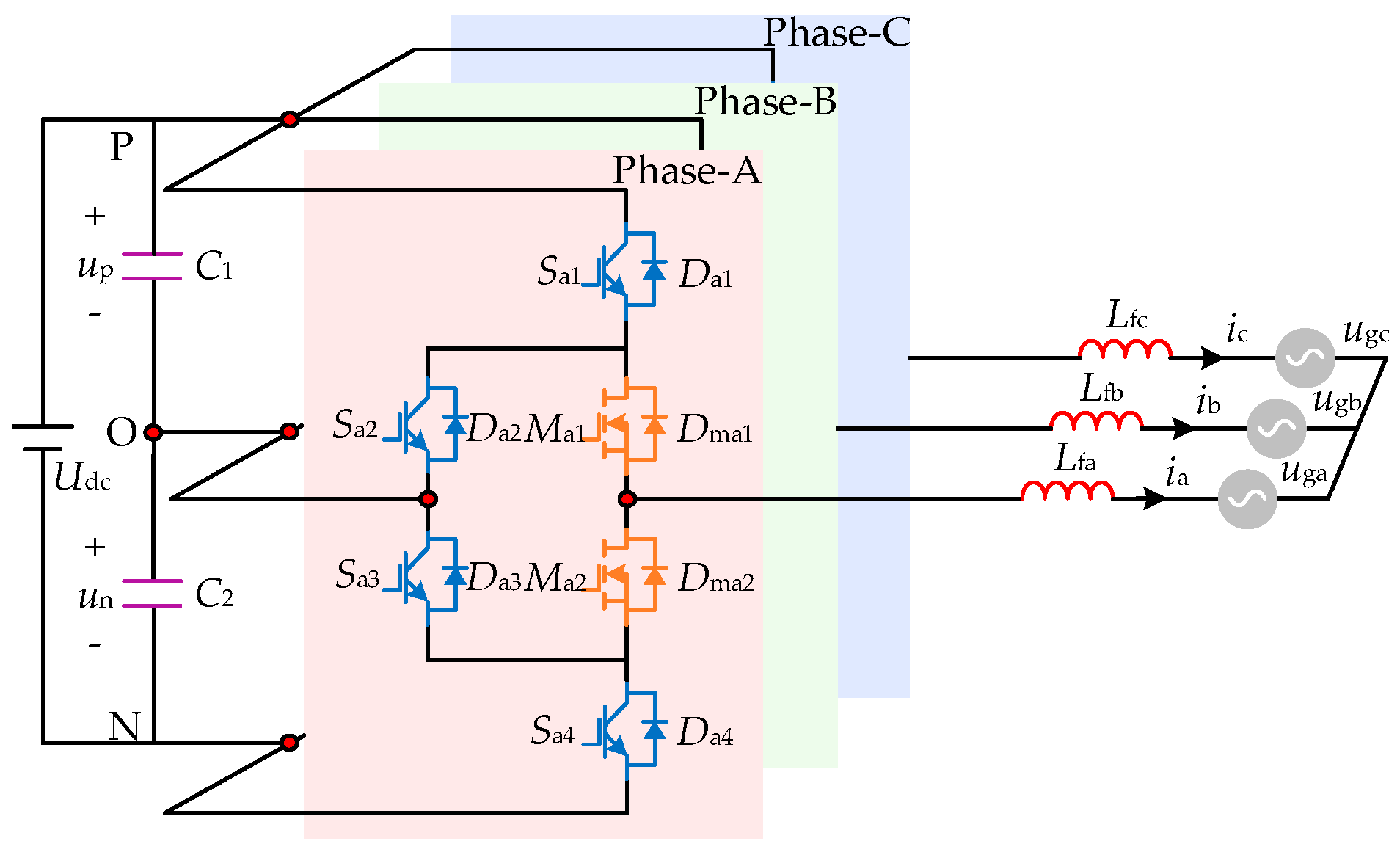
2. Characteristics Analysis of HANPC Converter in Faulty Conditions

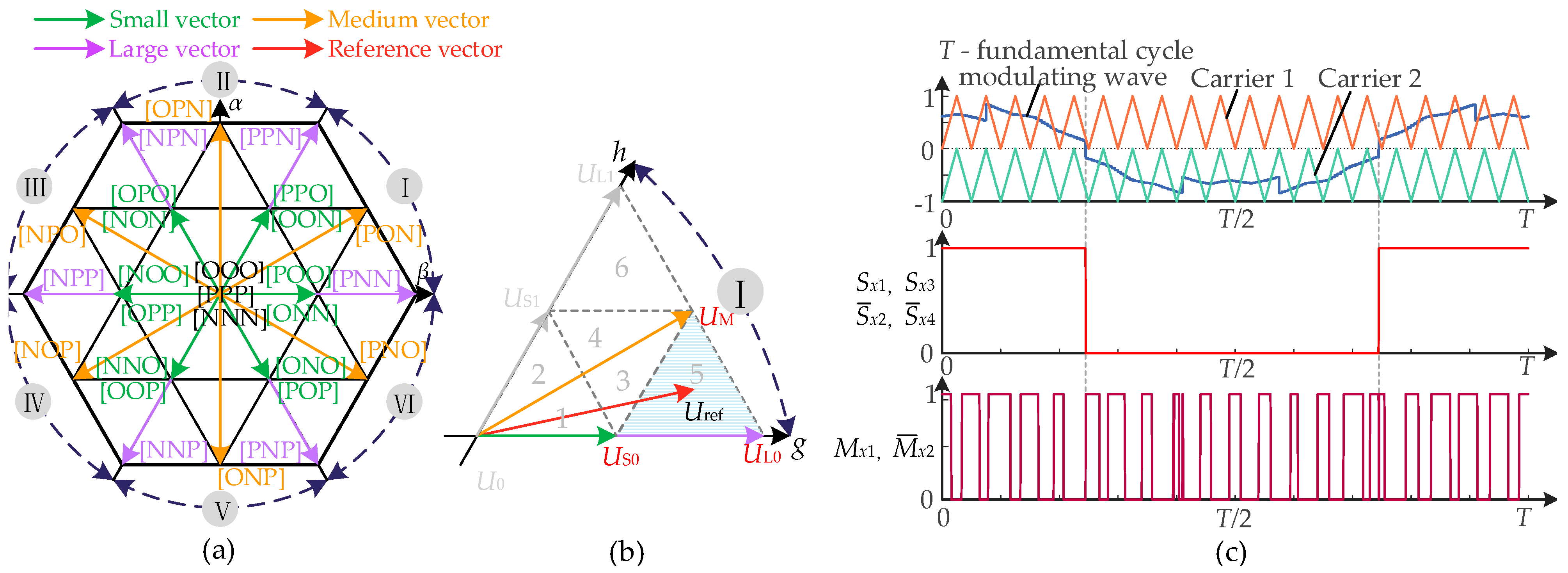
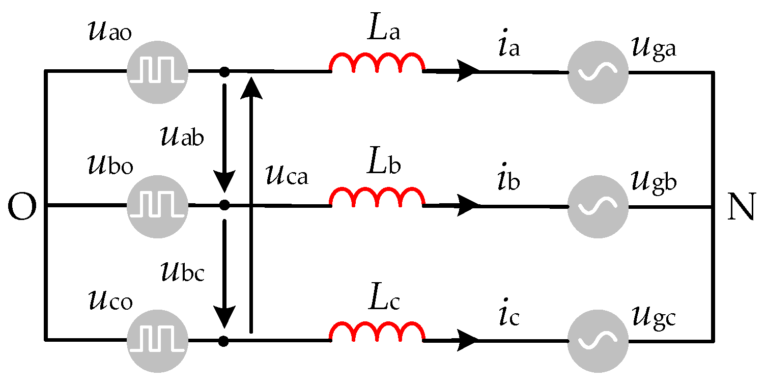
2.1. Modulation Description for HANPC

The switching principles of the HANPC converters are given in

Table 1. Switching principles for HANPC converters.

Switching State	Gate Sequence						Output Voltage Level
	Mx1	Mx2	Sx1	Sx2	Sx3	Sx4
[P]	1	0	1	0	1	0	Udc/2
[O−]	0	1	1	0	1	0	0
[O+]	1	0	0	1	0	1	0
[N]	0	1	0	1	0	1	−Udc/2

. Each phase leg of the converters can obtain the switching state [P], [O₊], [O₋], or [N]. The switching states [P] and [N] represent the output voltage levels of the corresponding phase leg, which are U_dc/2 and −U_dc/2, respectively. The switching states [O₊] and [O₋] represent the output voltage levels of the corresponding phase leg that are 0. For example, When the switches M_x1, S_x1, and S_x3 are turned on while other switches are turned off, the switching state [P] of phase-x leg can be obtained. In this condition, the output voltage of phase-x leg is U_dc/2.

Figure 2 shows the modulation of the HANPC converters [33]. The adopted modulation is a carrier-based space vector PWM. The method is based on the 60° g-h coordinated system, as shown in Figure 2b. It calculates the dwell time of selected vectors in each sector and equivalently converts it into duty cycles for generating the modulation waveform. By comparing the generated modulation wave with the cascaded carrier, gate signals for the switches can be obtained, as shown in Figure 2c. It is observed that all the high frequency actions occur in the SiC switches, while the Si switches operate at a fundamental frequency.

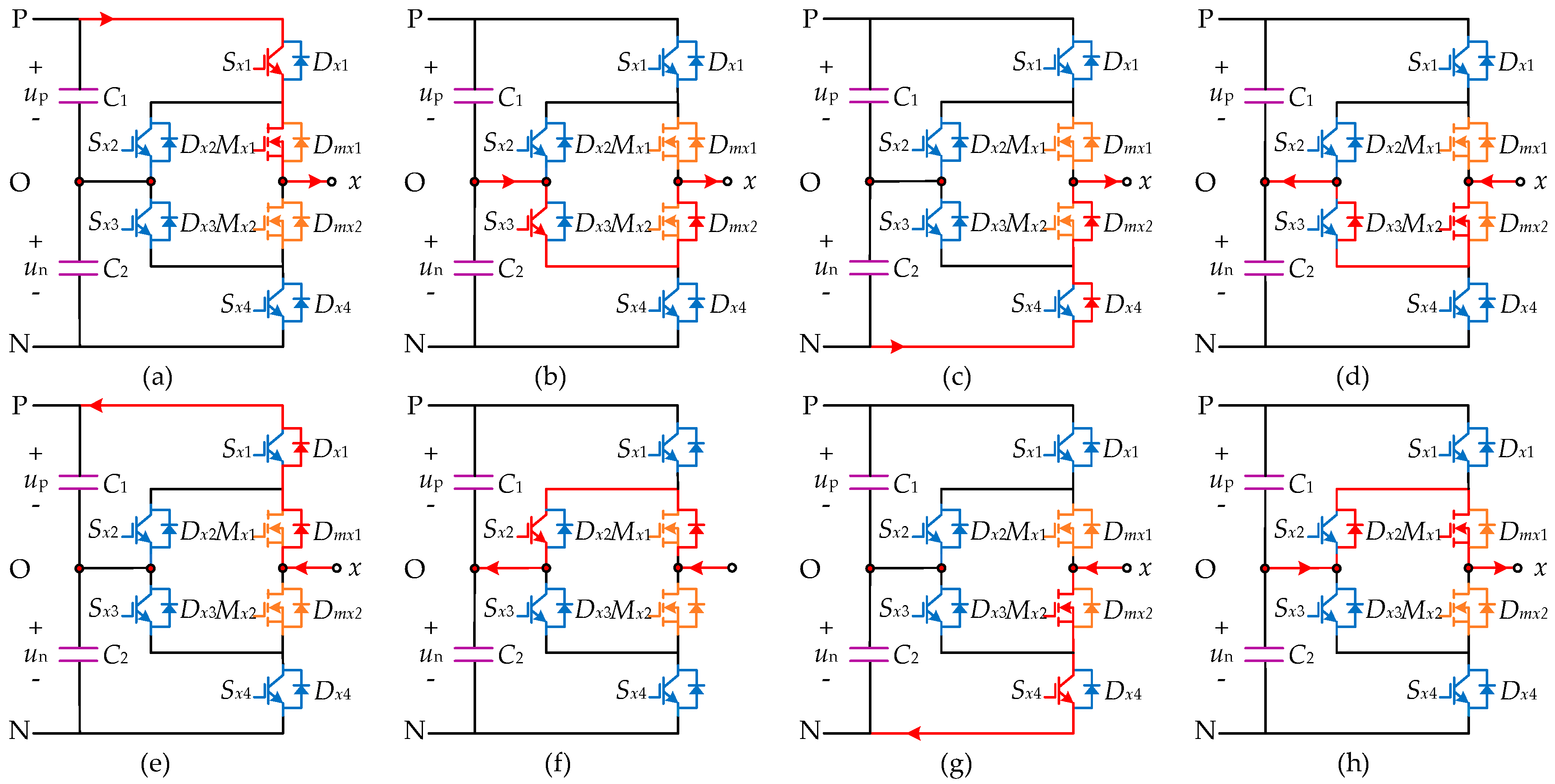
2.2. Effect of the Fault on Operation Mode of the Converter

HANPC converters have 8 operation modes, as shown in Figure 3, where the phase leg has four switching states associated with a corresponding positive or negative current path. Based on the operation modes for the phase legs of HANPC converters, the modulation range for each switch in the phase leg under the operation conditions of the unit power factor can be delineated, as shown in Figure 4. The region where the switch participates in the modulation is marked with colored rectangles. It is represented by the subgraphs in Figure 3a–h, which correspond to the related operation mode. For example, in interval [(a), (b)] (i_invx > 0), the phase-x leg performs transitions between mode 1 (Figure 3a) and mode 2 (Figure 3b). In this condition, the switches S_x1 (x = A, B, C) and S_x3 remain in the ON state, and the M_x1 and Mx₂ switches operate at high frequency. Additionally, in Figure 4, the angle of the output voltage u_invx leading the grid voltage u_gx is φ and the output current i_invx is in phase with the grid voltage u_gx.

In interval [(a), (b)], the current path of operation mode 1 is affected when the OC fault occurs in M_x1 or S_x1, as shown in Figure 3a. The current path of operation mode 2 is affected when the OC fault occurs in S_x3, as shown in Figure 3b. For [(c), (h)], only the OC fault at M_x1 would block the current path without regard to the diode fault, as shown in Figure 3h.

In interval [(f), (g)], only the OC fault at S_x2 would block the current path of operation mode 6 without regard to the diode fault, as shown in Figure 3f. The current path of operation mode 7 is affected when the OC fault occurs in M_x2 or S_x4, as shown in Figure 3g.

In the interval [(e), (d)], only the OC fault at M_x2 would block the current path without regard to the diode fault, as shown in Figure 3d. The range of [(c), (h)] and [(e), (d)] is relatively narrow. Consequently, the regions where M_x1, S_x1, and S_x3 participate in the modulation almost overlap. It is the same for M_x2, S_x2, and S_x4.

2.3. Behavior of Varying Electrical Quantities

If the current path in a specific operating mode of the HANPC is blocked due to the failure of the switch, the waveform of the output voltage will be altered, and the current waveform will become distorted. Given the structural symmetry of the three-phase HANPC converter, the behavior of output voltage and current are analyzed when an OC fault occurs at M_a1, S_a1, or S_a3.

Figure 5 shows the output current and voltage of HANPC converters under fault conditions, where t_F represents the time of fault occurrence. The “fault zero region (FZR)” is defined as the interval in which the phase current either decreases to or stabilizes near zero following an OC switch fault, as shown in Figure 5a (highlighted by the red-shaded area). The current in the zero region satisfies −Ith < i < Ith. For the design of the specific value of Ith, please refer to Section 3.4. When the OC fault occurs during interval [(a), (b)], the state [P] of the phase-A leg cannot be obtained under the OC fault at M_a1, and the current path changes from “S_a1-M_a1” to “D_a1-D_ma1 and S_a3-D_ma2”. In this condition, the switching state of the phase-A leg is forcibly clamped to [O]. A similar behavior is observed when the fault occurs at S_a1. As a result, the characteristics of output current and voltage exhibit a high degree of similarity. Specifically, the current in phase A becomes significantly distorted, rapidly decreasing in a linear manner toward zero. In the region where the current decreases linearly (R_cd), the output voltage level of the phase-A leg is clamped to 0. In contrast, the original output voltage level 0 is replaced by −U_dc/2 in R_cd when the OC fault occurs at S_a3. Furthermore, as shown in Figure 5, the voltage of the phase-A leg is floating within FZR. It is not considered that the fault occurs in the intervals [(c), (h)] and [(e), (d)] because these intervals close to the current zero region and that range is narrow.

When an OC fault occurs at M_a1 or S_a1, the positive current region becomes the fault zero region, while the waveforms in the negative current region are not affected. In contrast, when an OC fault occurs at S_a3, the positive current region is characterized by the presence of both a fault-zero region and a positive current distortion region. Additionally, the output voltage level of the faulty phase-leg is also floating within FZR.

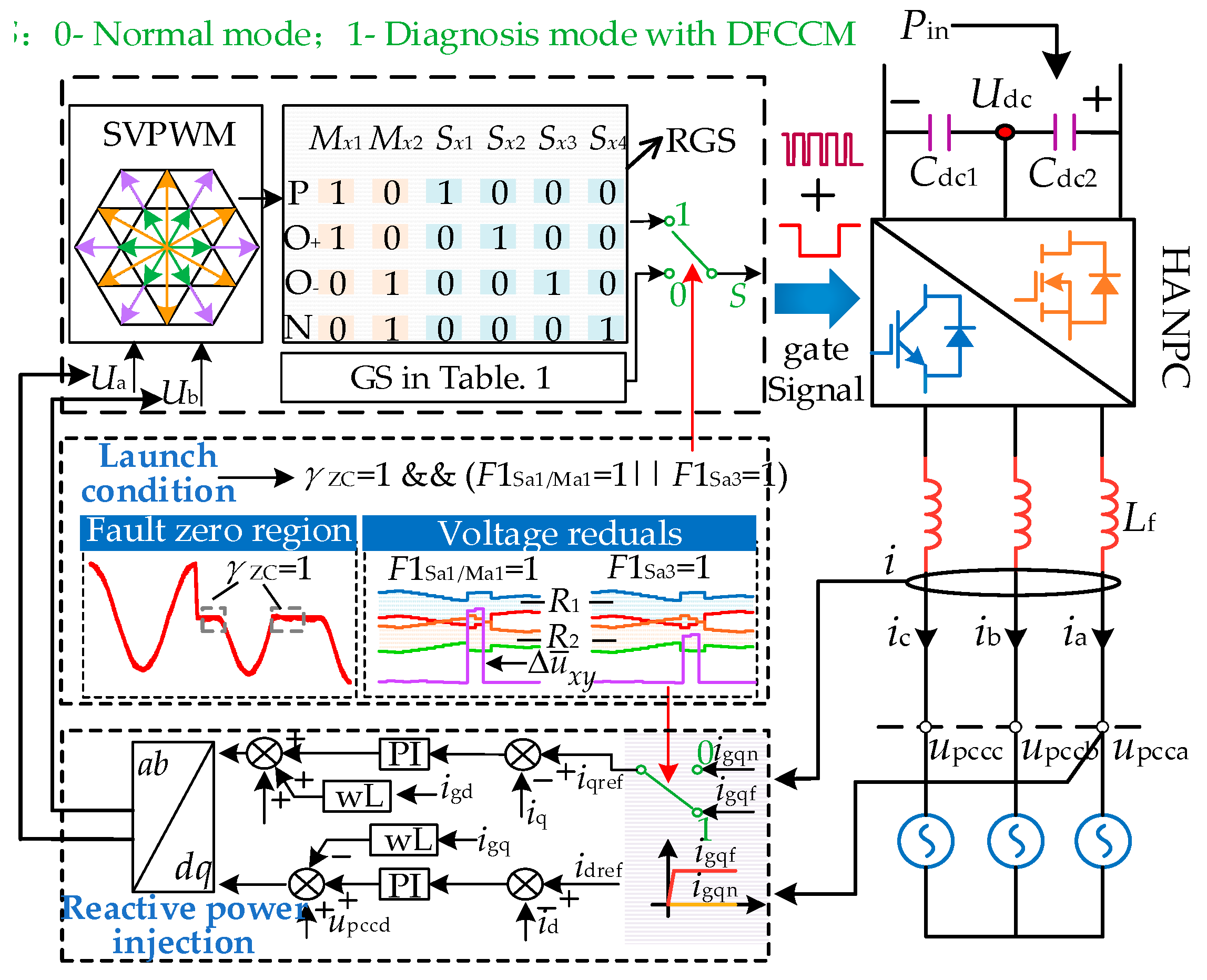
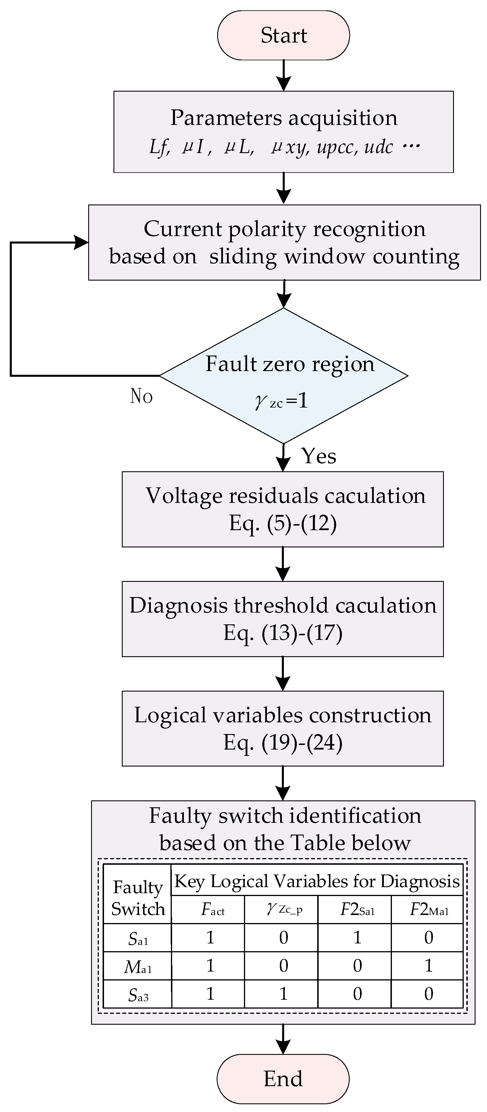
3. The Proposed Fault Diagnosis Method

As analyzed in Section 2, to achieve the faulty switch location by relying on the exiting electrical signals, several challenges must be addressed.

(1) The output voltage and current of the phase-A leg under an OC fault at M_x1 are similar to those under a fault at S_x1. This similarity makes it difficult to distinguish between M_x1 and S_x1 using conventional electrical characteristics.

(2) When an OC fault occurs at M_x1 or S_x1 in the negative current region, no linear current-decrease is observed. Instead, a fault zero region appears, during which the phase-leg voltage floats, making a voltage-based identification method ineffective.

To address these issues, the differentiated fault characteristic construction method (DFCCM) is proposed, as shown in Figure 6. The DFCCM is activated if the condition (γ_ZC = 1 && (F1_Sa1/Ma1 = 1 || F1_Sa3 = 1)) is satisfied. The “&&” represents logical AND, while the “||” represents logical OR. For a more detailed definition of other symbols in Figure 6, please refer to Section 3.5 of Section 3. The implementation process of the DFCCM is described as follows. First, a reactive current is injected to adjust the region where the switch participates in the modulation, thereby restoring the linear current-decrease region under the OC fault at M_x1 or S_x1. Subsequently, the neutral current path is reconfigured by using rearranged gate sequences (RGS) different from those in Table 1. This effectively alters the voltage and current characteristics of the faulty phase. Finally, the voltage residuals are utilized as the primary diagnostic variable, and the current polarity state serves as an auxiliary diagnostic variable. These variables are integrated to establish the fault location criterion.

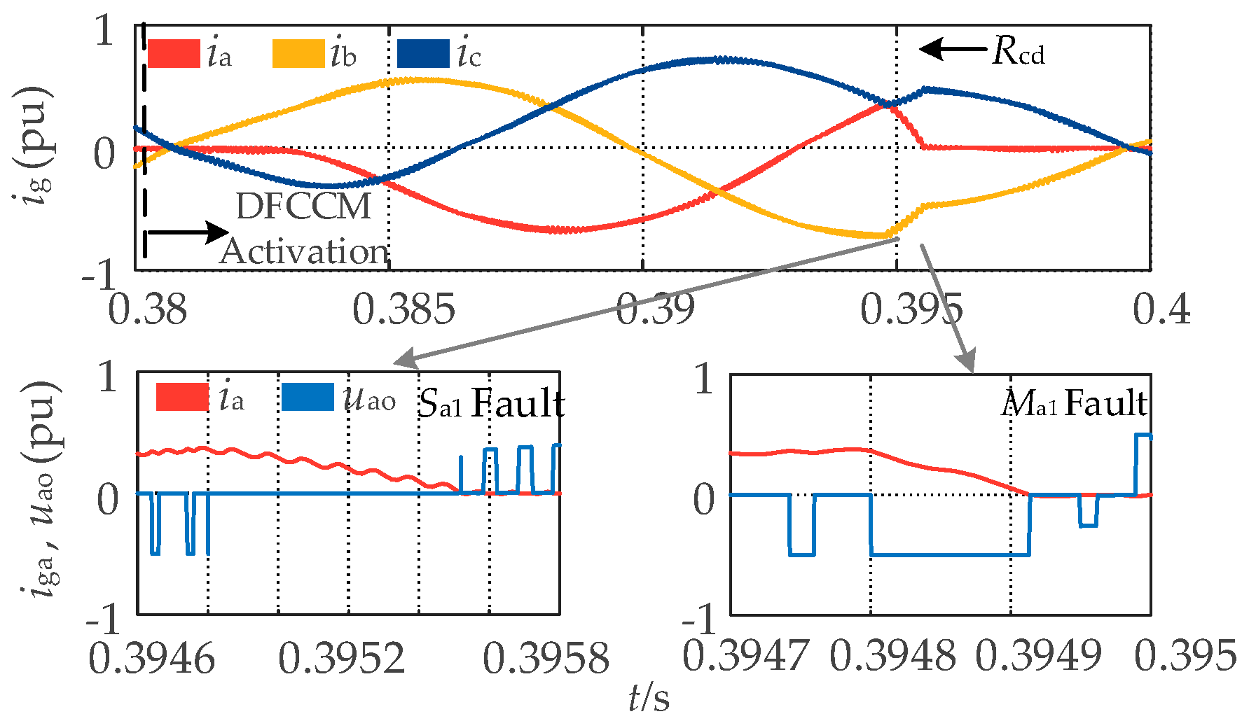
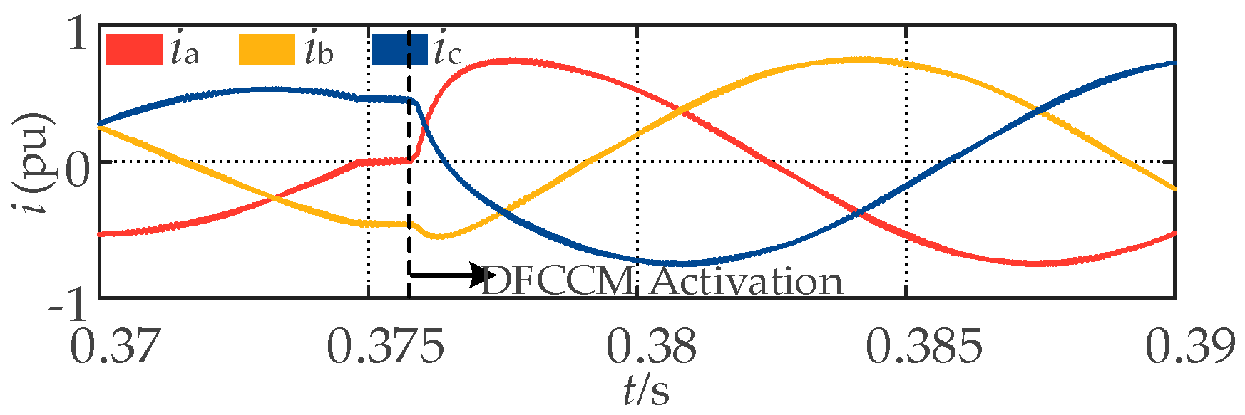
3.1. Behavior of Varying Electrical Quantities with DFCCM

The current and voltage waveforms in the case of an S_a1 fault or M_a1 fault are shown in Figure 7, and the current waveform in the case of an S_a3 fault is shown in Figure 8. Compared to the waveforms in Figure 5, the DFCCM introduces clear differences in the current and voltage characteristics under different faulty switches.

Specifically, for the S_a1 fault, the output voltage level of the phase leg is clamped to 0 in the region where the current decreases linearly. In contrast, for the M_a1 fault, the output voltage level is clamped to −U_dc/2. Notably, in the case of the S_a3 fault, there is no linear current-decrease region observed in the phase-A current. Instead, it exhibits a state transition from the FZR to the positive current region following the activation of the DFCCM.

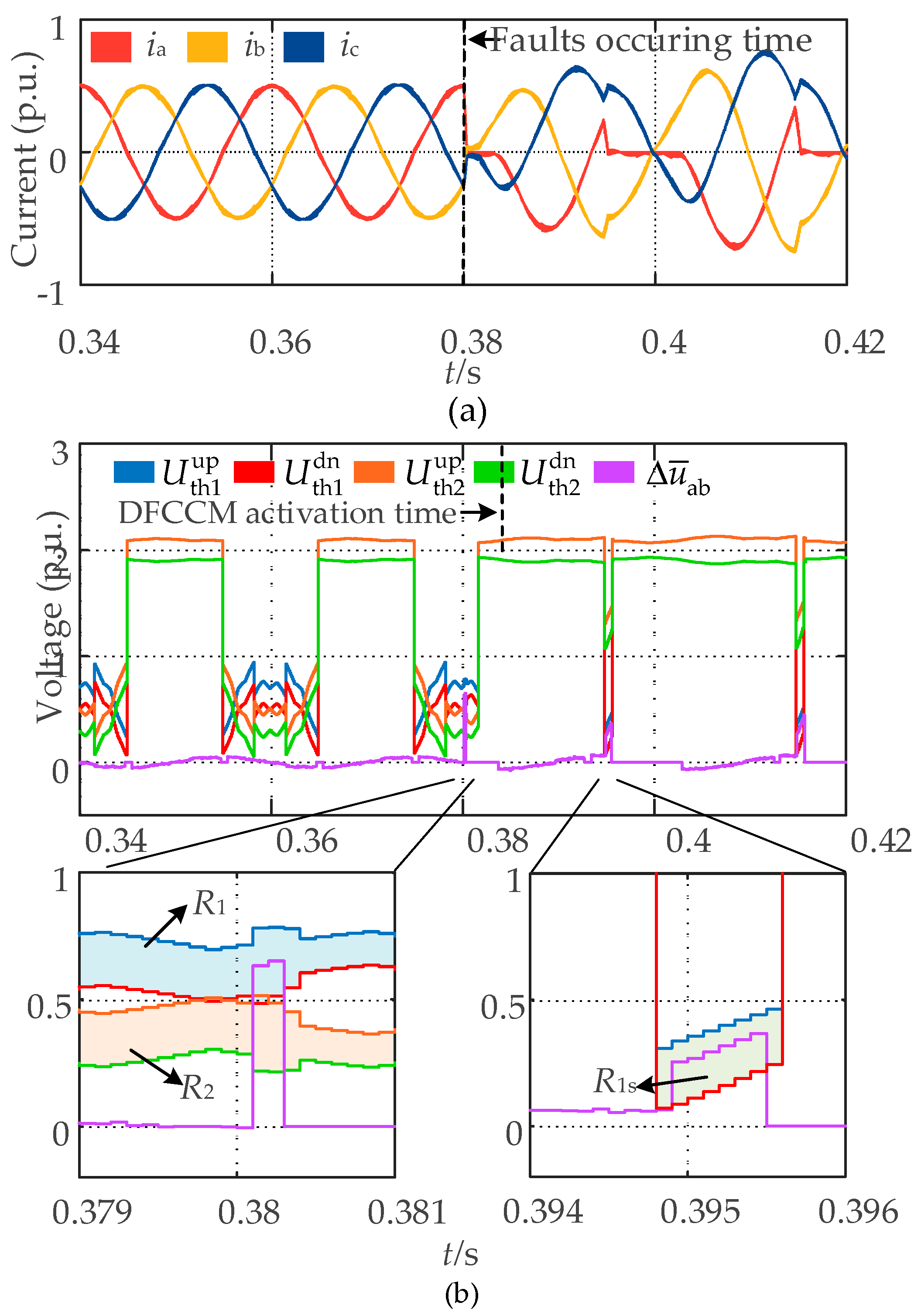
3.2. Generalized Voltage Residuals Model Based on the Variation of Pulse Equivalent Area

Based on the above analysis, within the linear current-decrease region, the output voltage of the faulty leg is clamped to a fixed level under an S_a1 or M_a1 fault. This leads to a large difference between the reference and actual output voltage (i.e., voltage residuals). This section develops a voltage residuals model and introduces a physical metric, “the variation of the pulse equivalent area”, to quantify the voltage residuals caused by switch faults. It reveals the mechanism by which the faulty switch affects the voltage residual, providing an important theoretical foundation for fault diagnosis.

(1)

The variation in pulse equivalent area before and after the switch OC fault

OC faults at S_a1 and M_a1 are given as examples to show the variation of the pulse equivalent area, respectively. Figure 9a shows the fault operation mode of the phase-A leg under the S_a1 fault, where the dwelling time of the voltage vectors [ONO], [ONP], [OOP], and [POP] are expressed as T₁l₁/2, T₂, T₃, and T₁l₂/2, respectively. Here, l₁ = (1 + k) and l₂ = (1 − k), and k represents the balance factor of neutral-point voltage. It is observed that the forward conduction path of the current i_a transitions from “S_a1-M_a1” to “D_a2-M_a1”, resulting in the operation state of phase-A leg shifting from “[P]” to “[O]”. The small vector [POP] fails and is replaced by the small vector [OOP].

In addition, as shown in Figure 9a, the pulse equivalent area for phase A under normal and fault conditions is expressed as

$$\left\{\begin{array}{l}{S}_{\mathrm{Sa}1\_\mathrm{eq}}^{\mathrm{nor}}={\displaystyle \frac{T_1}{2}}(1-k)\\ S_{\mathrm{Sa}1\_\mathrm{eq}}^{\mathrm{fault}}=0\end{array}\right.$$

(1)

Further, the variation in the pulse equivalent area of phase A before and after the S_a1 fault (i.e., the grey-shaded region in Figure 9a) is obtained as

$$S_{\mathrm{Sa}1\_\mathrm{eq}}={\displaystyle \frac{T_1}{2}}(1-k)$$

(2)

Figure 9b shows the fault operation mode of the phase-A leg under the M_a1 fault. As seen, the forward conduction path of i_a is “S_a1-M_a1” in the state [P] of the phase leg under normal conditions, but it transitions from “S_a1-M_a1” to “D_a4-D_ma2” under fault conditions. Similarly, the forward conduction path of i_a is “D_a2-M_a1” in the state [O] of the phase leg under normal conditions, but it transitions from “D_a2-M_a1” to “D_a4-D_ma2” under fault conditions. The phase-A leg is forcibly constrained to operate in the [N] state. Consequently, the unreachable vectors [ONO], [ONP], [OOP], and [POP] are replaced by [NNO], [NNP], [NOP], and [NOP], respectively.

In addition, as shown in Figure 9b, the pulse equivalent area for phase A under normal and fault conditions can be expressed as

$$\left\{\begin{array}{l}{S}_{\mathrm{Ma}1\_\mathrm{eq}}^{\mathrm{nor}}={\displaystyle \frac{T_1}{2}}(1-k)\\ S_{\mathrm{Ma}1\_\mathrm{eq}}^{\mathrm{fault}}=-(T_1+T_2+T_3)\end{array}\right.$$

(3)

Further, the variation in the pulse equivalent area of phase-A before and after the M_a1 fault (i.e., the grey-shaded region in Figure 9b) is obtained as

$$\Delta S_{\mathrm{Ma}1\_\mathrm{eq}}={\displaystyle \frac{T_1}{2}}(1-k)+T_{\mathrm{s}}$$

(4)

(2)

Generalized voltage residuals model

At the n-th sampling instant, within the linear current-decrease region, the moving averages of the actual phase voltage, expected phase voltage, and voltage residual for the HANPC converter can be expressed as

$$\left\{\begin{array}{c}{\overline{u}}_{x\mathrm{o}}(n)={\displaystyle \frac{1}{T_{\mathrm{s}}}}{\displaystyle {\int }_{t(n-1)}^{t(n)}{u}_{x\mathrm{o}}\mathrm{d}t}\\ {\overline{u}}_{x\mathrm{o}}^{*}(n)={\displaystyle \frac{1}{T_{\mathrm{s}}}}{\displaystyle {\int }_{t(n-1)}^{t(n)}{\overline{u}}_{x\mathrm{o}}^{*}\mathrm{d}t}\\ \Delta {\overline{u}}_{x\mathrm{o}}(n)={\overline{u}}_{x\mathrm{o}}^{*}(n)-{\overline{u}}_{x\mathrm{o}}(n)\end{array}\right.$$

(5)

Similarly, the moving average of the actual line-to-line voltage ${\overline{u}}_{xy}(n)$, expected line-to-line voltage ${\overline{u}}_{xn}^{*}(n)$, and line-to-line voltage residual $\Delta {\overline{u}}_{xy}(n)$ can be defined. The definition follows the same form as in Equation (5).

Based on Kirchhoff’s law and the equivalent circuit of the grid-tied HANPC converters in Figure 10, the actual line-to-line voltage between the phase leg is expressed as

$${\overline{u}}_{xy}(n)={\displaystyle \frac{1}{T_{\mathrm{s}}}}{\displaystyle {\int }_{t(n-1)}^{t(n)}(u_{xy}+\frac{\mathrm{d}{i}_x}{\mathrm{d}t}{L}_x}-{\displaystyle \frac{\mathrm{d}{i}_y}{\mathrm{d}t}}{L}_{\mathrm{y}})$$

(6)

To enable the computation of (6) using existing electrical signals in the controller, it is discretized as follows.

$$\begin{array}{ccc}{\overline{u}}_{xy}(n)& =& {\displaystyle \frac{1}{2}}[u_{xy}(n)+u_{xy}(n-1)]+{\displaystyle \frac{1}{T_{\mathrm{s}}}}\{L_x[i_x(n)-i_x(n-1)]-L_y[i_y(n)-i_{\mathrm{y}}(n-1)]\}\hfill \\ & =& {\overline{u}}_{x\mathrm{o}}(n)-{\overline{u}}_{y\mathrm{o}}(n)\hfill \end{array}$$

(7)

where L_x and L_y denote the filter inductance of phase-x and phase-y, respectively. i_x (n) and i_y (n) denote the currents of phase-x and phase-y at n-th sampling moment.

Further, ${\overline{u}}_{x\mathrm{y}}^{*}(n)$ can be expressed as

$${\overline{u}}_{x\mathrm{y}}^{*}(n)={(-1)}^r{\displaystyle \frac{U_{\mathrm{dc}}}{2}}{d}_x-{(-1)}^q{\displaystyle \frac{U_{\mathrm{dc}}}{2}}{d}_{\mathrm{y}}$$

(8)

where the dwelling duty d_x is defined as the ratio of dwelling time of the states [P] or [N] to the switching period. If the phase-x leg operates in the [P] and [O] during a switching period, r is assigned a value of 0. Conversely, if it operates in the [N] and [O], r is assigned a value of 1. The meanings of d_y and q are analogous to those of d_x and r.

In the following, the OC fault at S_a1 is given as an example to derive the quantitative expression for the voltage residual. In case of an S_a1 fault, Equation (9) can be obtained.

$$\left\{\begin{array}{c}{\overline{u}}_{\mathrm{ab}}(n)={\overline{u}}_{\mathrm{ao}}(n)-{\overline{u}}_{\mathrm{bo}}(n)\\ {\overline{u}}_{\mathrm{ab}}^{*}(n)={\overline{u}}_{\mathrm{ao}}^{*}(n)-{\overline{u}}_{\mathrm{bo}}^{*}(n)\end{array}\right.$$

(9)

Furthermore, the following equation can be derived as

$$\Delta {\overline{u}}_{\mathrm{ab}}(n)=\Delta {\overline{u}}_{\mathrm{ao}}(n)$$

(10)

Based on the variation of the pulse equivalent area in Figure 9a, the moving average of the phase-A output voltage can be calculated as follows, including both pre-fault and post-fault conditions.

$$\left\{\begin{array}{l}{u}_{\mathrm{ao}}^{\mathrm{pre}}(n)={\displaystyle \frac{U_{\mathrm{dc}}}{2}}\cdot {\displaystyle \frac{T_1}{2}}(1-k)={\displaystyle \frac{U_{\mathrm{dc}}}{2T_{\mathrm{s}}}}\Delta S_{\mathrm{Sa}1\_\mathrm{eq}}\\ u_{\mathrm{ao}}^{\mathrm{post}}(n)=0\end{array}\right.$$

(11)

By combining Equation (5) with Equation (11), Equation (12) is derived as

$$\Delta {\overline{u}}_{\mathrm{ab}}(n)={\displaystyle \frac{U_{\mathrm{dc}}}{2T_{\mathrm{s}}}}\Delta S_{\mathrm{Sa}1\_\mathrm{eq}}$$

(12)

Equation (12) reveals that the line-to-line voltage residual can be quantified by the variation in the pulse equivalent area. The quantification expressions for voltage residuals under other switch fault conditions can be derived using the same method.

To better illustrate, the voltage residuals and their corresponding threshold regions are given in Figure 11. It can be observed that when faults occur at Sa1, the voltage residuals exhibit significant changes and enter the threshold region R1. After the DFCCM strategy is activated, the residuals further transition into threshold region R1s.

3.3. Current Polarity Recognition

To identify the current polarity states under fault conditions, a recognition method based on sliding window counting is proposed, as shown in Figure 12. The i_x[n] denotes current sampling at the n-th sampling moment in the controller. If the phase current i_x[n] ∈ [−Ith, Ith], it is classified as a zero current state “0”; if i_xo[n] > Ith, it is classified as a positive current state “+”. A sliding window is employed to process the data samples of the current, obtaining the count of each type of polarity current sample within the sliding window. In the digital controller, the sliding window is represented by the array i[m], where m denotes the length of the sliding window.

The sliding window is updated with each sampling moment. It is evenly divided into a front window (FW) and a rear window (RW). Initially, the number of positive current states in the front window is denoted as C_p1, and the number of zero current states is denoted as C_o1. Similarly, the initial number of positive and zero current states in the rear window are denoted as C_p2 and C_o2, respectively. As the window slides, if the current sampling data exiting the front window corresponds to the positive current state, the C_p1 is reduced by 1. If the current sampling entering the front window corresponds to a zero current state, the C_o1 is increased by 1. Similar operations are performed when the data corresponds to other current states. The operations for the rear window are analogous to those for the front window and are not elaborated here. When C_o2 is greater than the counting threshold N_tho2, it indicates the FZR is recognized. When C_o1 > N_tho1 and C_p2 > N_thp2, it indicates that the state transition process from FZR to the positive current region is recognized. N_tho1 and N_thp2 denote corresponding counting thresholds. The design of counting thresholds and the establishment of logical variables for current states are discussed in Section 3.4 and Section 3.5.

3.4. Threshold Selection

A well-designed threshold is crucial for ensuring the effectiveness of the diagnostic method, as it directly influences both the accuracy and speed of the diagnosis. The thresholds discussed in this paper include the voltage threshold, zero current threshold, counting threshold, and window length. The process of designing these thresholds is elaborated in the following.

(1)

Adaptive voltage threshold

To improve diagnostic robustness, it is necessary to account for the inductance parameter errors, sampling errors, and effect of switch dead-time on the diagnostic variable $\Delta {\overline{u}}_{xy}(n)$. Taking the above factors into consideration, the voltage error can be expressed as [34]

$$\Delta {\overline{u}}_{xy\_\mathrm{error}}={\displaystyle \frac{1}{T_{\mathrm{s}}}}{\mu }_{\mathrm{L}}\left|i_x(n)-i_x(n-1)\right|+{\displaystyle \frac{1}{T_{\mathrm{s}}}}{\mu }_{\mathrm{L}}\left|i_{\mathrm{y}}(n)-i_y(n-1)\right|+{\mu }_{xy}+{\displaystyle \frac{4}{T_{\mathrm{s}}}}{\mu }_{i}L+U_{\mathrm{dc}}{\displaystyle \frac{T_{\mathrm{dead}}}{T_{\mathrm{s}}}}$$

(13)

where μ_L denotes the inductance parameters errors; μ_i stands for the current sampling errors; μ_xy denotes the sampling errors of the grid line-to-line voltage; and T_dead denotes the dead-time of the switch.

Based on Equations (10) and (13), the adaptive voltage threshold regions are designed. These include regions R₁ and R₂ before DFCCM activation, and the regions R_1S and R_2S after its activation, which are expressed as

$$\left\{\begin{array}{l}{R}_1=[{\displaystyle \frac{U_{\mathrm{dc}}\Delta {S^{\prime }}_{\mathrm{sa}1}}{2T_{\mathrm{s}}}}-\Delta {\overline{u}}_{xy\_\mathrm{error}}, {\displaystyle \frac{U_{\mathrm{dc}}\Delta {S^{\prime }}_{\mathrm{sa}1}}{2T_{\mathrm{s}}}}+\Delta {\overline{u}}_{xy\_\mathrm{error}}]\\ R_2=[{\displaystyle \frac{U_{\mathrm{dc}}\Delta {S^{\prime }}_{\mathrm{Sa}3}}{2T_{\mathrm{s}}}}-\Delta {\overline{u}}_{xy\_\mathrm{error}}, {\displaystyle \frac{U_{\mathrm{dc}}\Delta {S^{\prime }}_{\mathrm{Sa}3}}{2T_{\mathrm{s}}}}+\Delta {\overline{u}}_{xy\_\mathrm{error}}]\\ R_{1\mathrm{S}}=[{\displaystyle \frac{U_{\mathrm{dc}}\Delta {S^{″}}_{\mathrm{Sa}1}}{2T_{\mathrm{s}}}}-\Delta {\overline{u}}_{xy\_\mathrm{error}}, {\displaystyle \frac{U_{\mathrm{dc}}\Delta {S^{″}}_{\mathrm{Sa}1}}{2T_{\mathrm{s}}}}+\Delta {\overline{u}}_{xy\_\mathrm{error}}]\\ R_{2\mathrm{S}}=[{\displaystyle \frac{U_{\mathrm{dc}}\Delta {S^{″}}_{\mathrm{Ma}1}}{2T_{\mathrm{s}}}}-\Delta {\overline{u}}_{xy\_\mathrm{error}}, {\displaystyle \frac{U_{\mathrm{dc}}\Delta {S^{″}}_{\mathrm{Ma}1}}{2T_{\mathrm{s}}}}+\Delta {\overline{u}}_{xy\_\mathrm{error}}]\end{array}\right.$$

(14)

where $\Delta {S^{\prime }}_{\mathrm{sa}1}$ and $\Delta {S^{\prime }}_{\mathrm{a}3}$ denote the variations in the area of the pulse sequence caused by the OC fault at S_a1/M_a1 and S_a3, respectively, before DFCCM activation. $\Delta {S^{″}}_{\mathrm{Sa}1}$ and $\Delta {S^{″}}_{\mathrm{Ma}1}$ denote the corresponding variations caused by the fault at S_a1 and M_a1 after DFCCM activation.

(2)

Zero current threshold

Ideally, the value of the current sample in the FZR should be zero. However, deviations inevitably arise due to the combined effects of sampling errors, noise, and harmonic interference. Considering these factors, the threshold for the FZR is calculated as

$$I_{\mathrm{th}}=k\sqrt{I_{\mathrm{d}\_\mathrm{ref}}^2+I_{\mathrm{q}\_\mathrm{ref}}^2}$$

(15)

where k denotes the current threshold scaling factor, with a value ranging from 0.05 to 0.1. I_{d_ref} and I_{q_ref} denote the reference active current and reactive current, respectively.

(3)

Counting threshold and the length of the sliding window

Based on the determined zero current threshold, the number of zero current states N_zc near the phase current zero-crossing under normal conditions can be calculated. The N_tho1 and N_tho2 are set greater than N_zc; otherwise, misdiagnosis may occur. Consequently, it is recommended to set N_tho1 and N_tho2 as

$$N_{\mathrm{tho}1}=N_{\mathrm{tho}2}=(1.5~3)N_{\mathrm{ZC}}$$

(16)

The length of the sliding window m must be at least 2N_tho1. The positive polarity counting threshold N_thp should be greater than half the length of the rear sliding window, which is expressed as

$$N_{\mathrm{thp}}\ge {\displaystyle \frac{1}{4}}m$$

(17)

3.5. Fault Location Criterion

In this subsection, some logic variables are established to develop the fault location criterion. The definitions of each logic variable are presented in detail below.

Based on the proposed current polarity recognition method, the logical variable for detecting FZR is defined as

$${\gamma }_{\mathrm{zc}}=\left\{\begin{array}{l}1 C_{\mathrm{o}2}\ge N_{\mathrm{tho}2}\\ 0 C_{\mathrm{o}2}<N_{\mathrm{tho}2}\end{array}\right.$$

(18)

where the value “1” means high level and “0” means low level. C_o2 denotes the number of zero current states in the rear window, and N_tho2 denotes the corresponding zero current threshold.

The logical variable for detecting the state transition process from the FZR to the positive current region is as follows:

$${\nu }_{\mathrm{zc}\_\mathrm{p}}=\left\{\begin{array}{l}1 C_{\mathrm{o}1}>N_{\mathrm{tho}1}\&\&C_{\mathrm{P}2}>N_{\mathrm{thp}2}\\ 0 \mathrm{else}\end{array}\right.$$

(19)

where C_o1 denotes the number of zero states in the front window, and N_tho1 denotes the corresponding zero current threshold. C_P2 denotes the number of positive current states in the rear window, and N_thp2 denotes the positive current threshold.

In the region where the current decreases linearly, the voltage residuals differ depending on the specific faulty switch. The logical variable for locating the faulty switch at S_a1 or M_a1 before DFCCM activation is defined as

$$F{1}_{\mathrm{Sa}1/\mathrm{Ma}1}=\left\{\begin{array}{l}1 \Delta {\overline{u}}_{\mathrm{ab}}\in R_1\\ 0 \Delta {\overline{u}}_{\mathrm{ab}}\notin R_1\end{array}\right.$$

(20)

where $\Delta {\overline{u}}_{\mathrm{ab}}$ line-to-line voltage residuals between phase A and phase B. The definition of R₁ is shown in Equation (14).

The logical variables for locating the faulty switch S_a3 is defined as

$$F{1}_{\mathrm{Sa}3}=\left\{\begin{array}{l}1 \Delta {\overline{u}}_{\mathrm{ab}}\in R_2\\ 0 \Delta {\overline{u}}_{\mathrm{ab}}\notin R_2\end{array}\right.$$

(21)

where the definition of R₂ is shown in Equation (14).

Upon detecting the fault zero region, and when F1_Sa1/Ma1 = 1 or F1_Sa3 = 1, the DFCCM is activated to ensure the accuracy of faulty switch localization. The logical variable for activating the DFCCM is defined as

$$F_{\mathrm{act}}=\left\{\begin{array}{l}1 D\&\&E\\ 0 \mathrm{else} \end{array}\right.$$

(22)

where D is expressed as γ_ZC = 1, while condition E is defined as (F1_Sa1/Ma1 =1) || (F1_Sa3 = 1). The symbol “&&” denotes logical AND operator, and “||” denotes logical OR operator.

Following the activation of the DFCCM, the logical variables for locating faulty switches S_a1 and M_a1 are defined as

$$F{2}_{\mathrm{Sa}1}=\left\{\begin{array}{l}1 \Delta {\overline{u}}_{\mathrm{ab}}\in R_{1\mathrm{S}}\\ 0 \Delta {\overline{u}}_{\mathrm{ab}}\notin R_{1\mathrm{S}}\end{array}\right.$$

(23)

$$F{2}_{\mathrm{Ma}1}=\left\{\begin{array}{l}1 \Delta {\overline{u}}_{\mathrm{ab}}\in R_{2\mathrm{S}}\\ 0 \Delta {\overline{u}}_{\mathrm{ab}}\notin R_{2\mathrm{S}}\end{array}\right.$$

(24)

where the definition of R_1S and R_2S is shown in Equation (14).

Building upon the combination of the logical variables described above, fault location criteria are formulated, as presented in Figure 13, which delineates the conditions under which the fault of a corresponding switch is anticipated. When all conditions in a given row of the table are simultaneously met, the switch corresponding to that row is identified as the faulty switch.

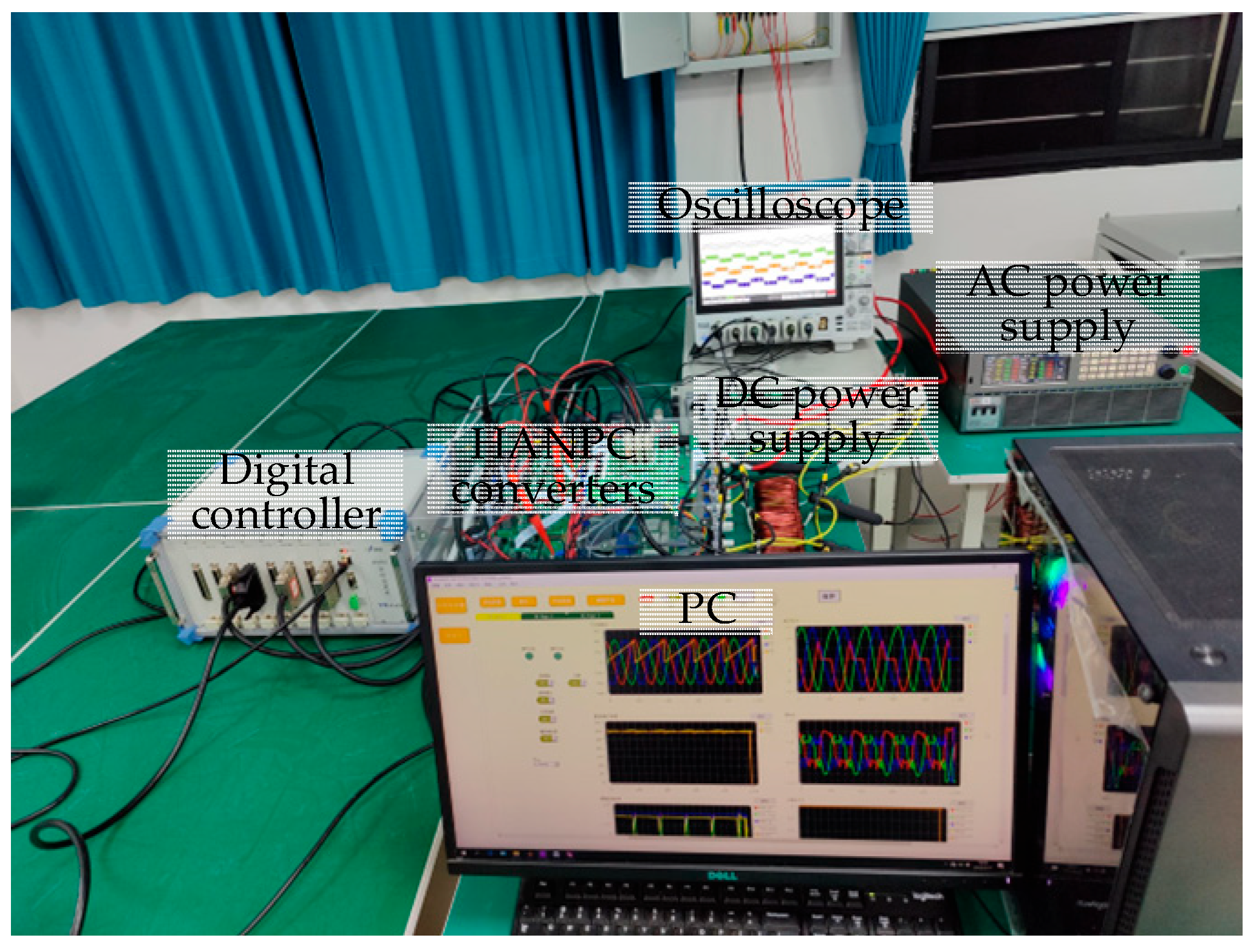
4. Experimental Results

To verify the effectiveness of the proposed fault diagnosis method, the experimental prototype of grid-tied HANPC converters is built, as shown in Figure 14. The experimental parameters are listed in

Table 2. Experimental parameters.

Parameters	Symbol	Value
DC input voltage	Udc	600 V
DC-link capacitor	C1, C2	1020 μF
AC filter inductor	L	6 mH
AC grid phase-voltage	Ux	150 V
Rated power	Prated	10 kW
Grid frequency	fg	50 Hz
Switching frequency	fs	10 kHz
Switching dead time	Tdead	2 μs

. Two groups of tests, including effectiveness and robustness verification of the proposed fault diagnosis method, are carried out. The OC fault in a power switch of an HANPC converter is realized by clamping the gate drive signal of the related switch to a low level. In the following experimental results, the value of the undrawn key logic variables for fault diagnosis is always zero (i.e., low level). i_x (x = a, b, c) denotes the output currents of the converter, and u_xo denotes the pole voltage of the converter. $U_{\mathrm{th}1}^{\mathrm{up}}$ denotes the upper boundary of the threshold region R₁ before DFCCM activation and that of the threshold region R_1S after DFCCM activation. $U_{\mathrm{th}1}^{\mathrm{dn}}$ denotes the lower boundary of the threshold region R₁ before DFCCM activation and that of the threshold region R_1S after DFCCM activation. Similarly, Uth2up and Uth2dn denote the upper and lower boundaries of the threshold regions R2 (before DFCCM activation) and R2S (after DFCCM activation), respectively.

4.1. Effectiveness Verification of Proposed Method

Four representative fault conditions are selected to verify the effectiveness of the proposed fault diagnosis method. In the following experimental results, the threshold region of the voltage residuals is dynamically adaptive, which takes into account the model calculation error and the modulation working interval, rather than the traditional fixed threshold. Meanwhile, the threshold region of the voltage residuals is set high in the non-working region of the corresponding switch, which effectively guarantees the robustness of fault diagnosis. Additionally, it should be noted that the overlap of the threshold regions R₁ and R₂ before activation of the DFCCM would cause misdiagnosis. After the activation of the DFCCM, the distance between threshold regions R_1s and R_2s is relatively large, addressing the issue of misdiagnosis caused by the overlap of the threshold region.

(1)

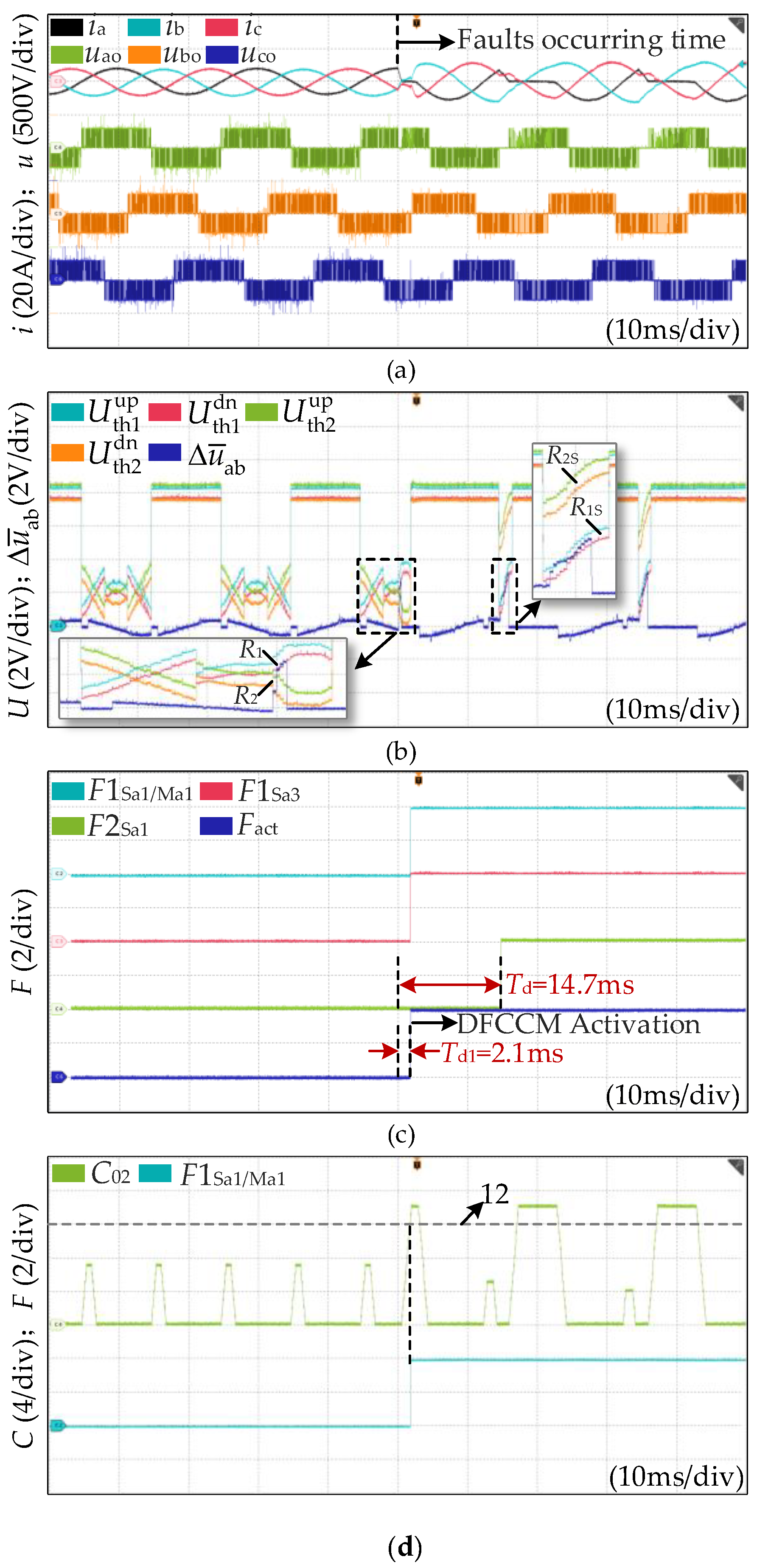
Case 1: The OC fault occurs at S_a1 when i_a > 0.

Figure 15 shows the experimental waveforms of case 1. As shown in Figure 15a, the phase-A current i_a begins to decrease linearly following the fault. Meanwhile, the voltage residual $\Delta {\overline{u}}_{\mathrm{ab}}$ enters both threshold regions R₁ and R₂ (Figure 15b) before DFCCM activation. This condition immediately triggers the first-stage diagnostic signals F1_Sa1/Ma1 and F1_Sa3 to a logic high state (Figure 15c), indicating a possible OC fault at S_a1, M_a1, or S_a3. As the current further decreases, it enters the fault zero region (FZR). The count variable C₀₂, representing the number of consecutive zero current samples within a sliding rear window, exceeds 12 (i.e., count threshold), confirming FZR detection. This fulfills the condition for activating the DFCCM, and logical variable F_act transitions to a logic high state. After the DFCCM is activated, the voltage residual $\Delta {\overline{u}}_{\mathrm{ab}}$ is re-evaluated against the updated threshold region R_1S, which is separated from R_2S to avoid region overlap. $\Delta {\overline{u}}_{\mathrm{ab}}$ subsequently enters R_1S [Figure 15b], triggering the second-stage diagnostic variable F2_Sa1 to a logic high state. Finally, all identification conditions for S_a1 are satisfied, and the fault is conclusively attributed to switch S_a1.

(2)

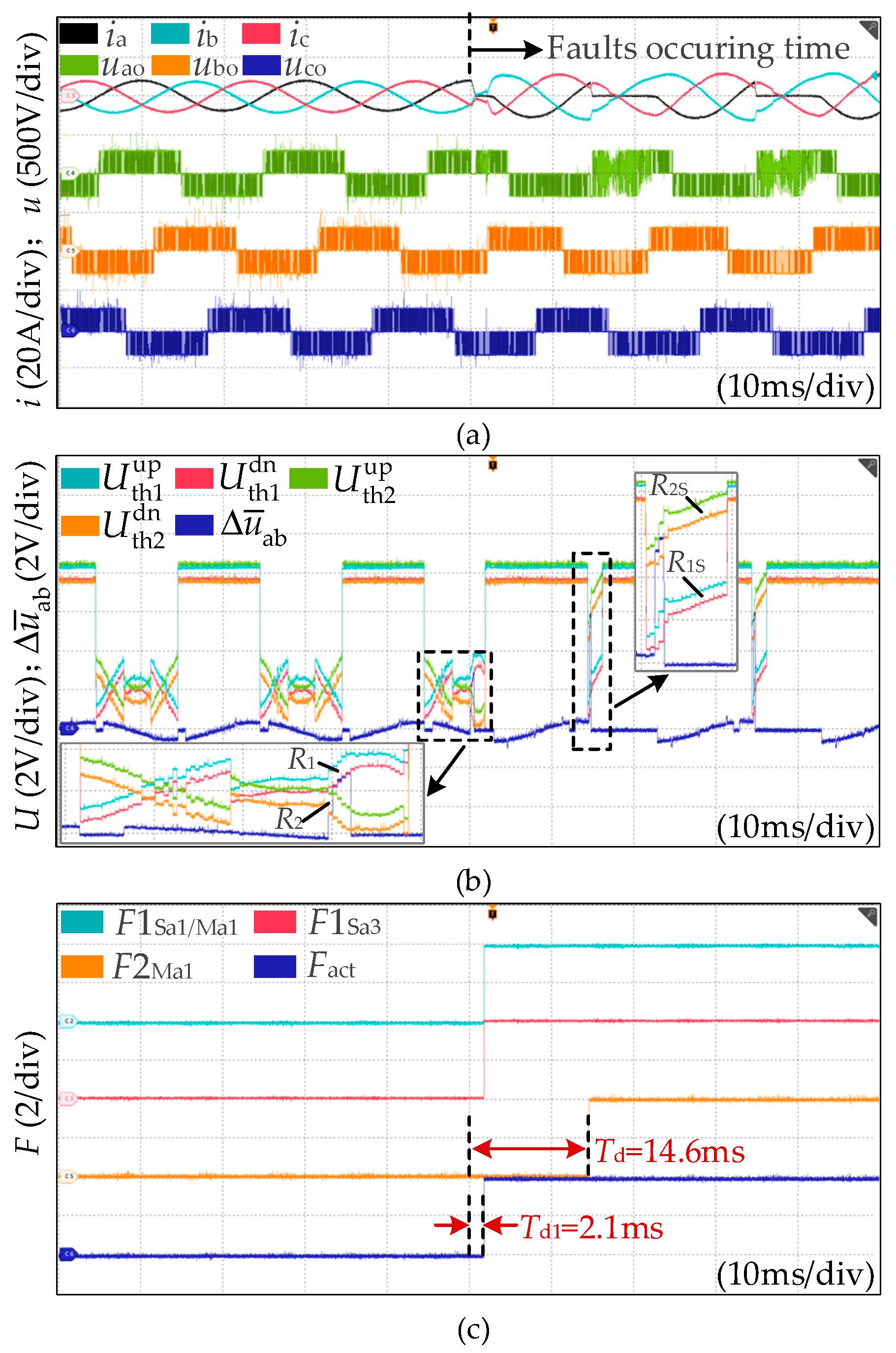
Case 2: The OC fault occurs at M_a1 when i_a > 0.

Figure 16 shows the experimental waveforms of case 2. As shown in Figure 16b, the voltage residual $\Delta {\overline{u}}_{\mathrm{ab}}$ enters both threshold R₁ and R₂ under post-fault conditions. This immediately drives the first-stage diagnostic signals F1_Sa1/Ma1 and F1_Sa3 to a logic high state, indicating a possible OC fault at S_a1, M_a1, or S_a3. When the FZR is identified, F_act is driven to a logic high state and the DFCCM is activated. After DFCCM activation, the voltage residual $\Delta {\overline{u}}_{\mathrm{ab}}$ enters the refined threshold region R_2S (Figure 16b), and the second-stage diagnostic variable F2_Ma1 is set high (Figure 16c). Finally, all fault location conditions for switch M_a1 are satisfied. Consequently, M_a1 is identified as the faulty switch.

(3)

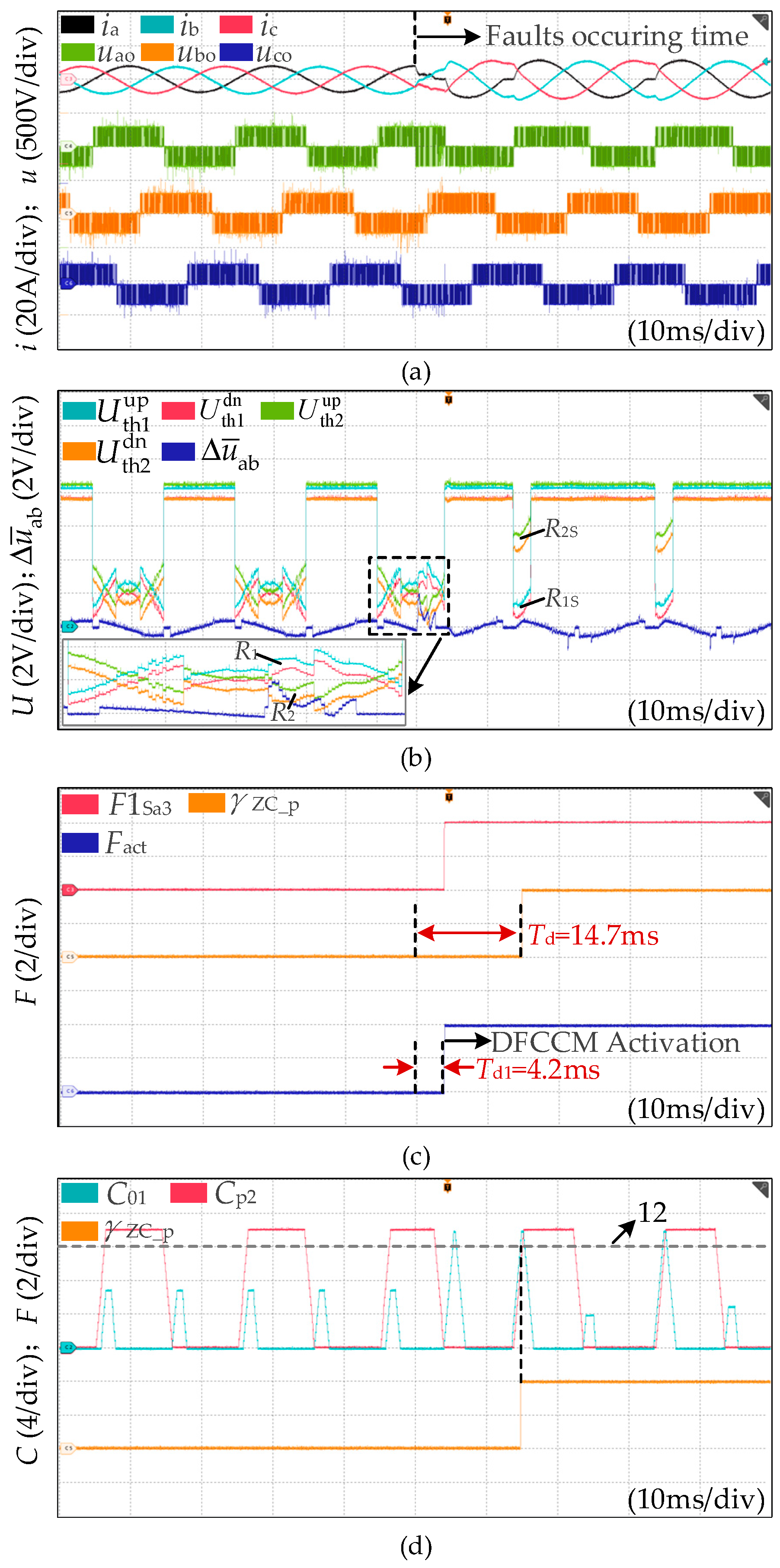
Case 3: The OC fault occurs at S_a3 when i_a > 0.

Figure 17 shows the experimental waveforms of case 3. As the fault current on phase A decreases linearly (Figure 17a), the voltage residual $\Delta {\overline{u}}_{\mathrm{ab}}$ enters only the threshold region R₂ (Figure 17b), and the F1_Sa3 is driven to a logic high state (Figure 17c). Once the FZR is detected, the DFCCM is activated to enhance diagnostic accuracy. Following activation, the counter variable of positive current state C_p2 exceeds 10 in the sliding rear window with the counter variable of the zero current state C₀₁ > 12 (Figure 17d). It indicates that the change process of current polarity from “0” state to “+” state is detected, and logic variable γ_{ZC_P} is driven to a logic high state. In addition, $\Delta {\overline{u}}_{\mathrm{ab}}$ does not enter the threshold regions R_1S and R_2S. According to the formulated fault location criterion, S_a3 is determined to be the faulty switch.

(4)

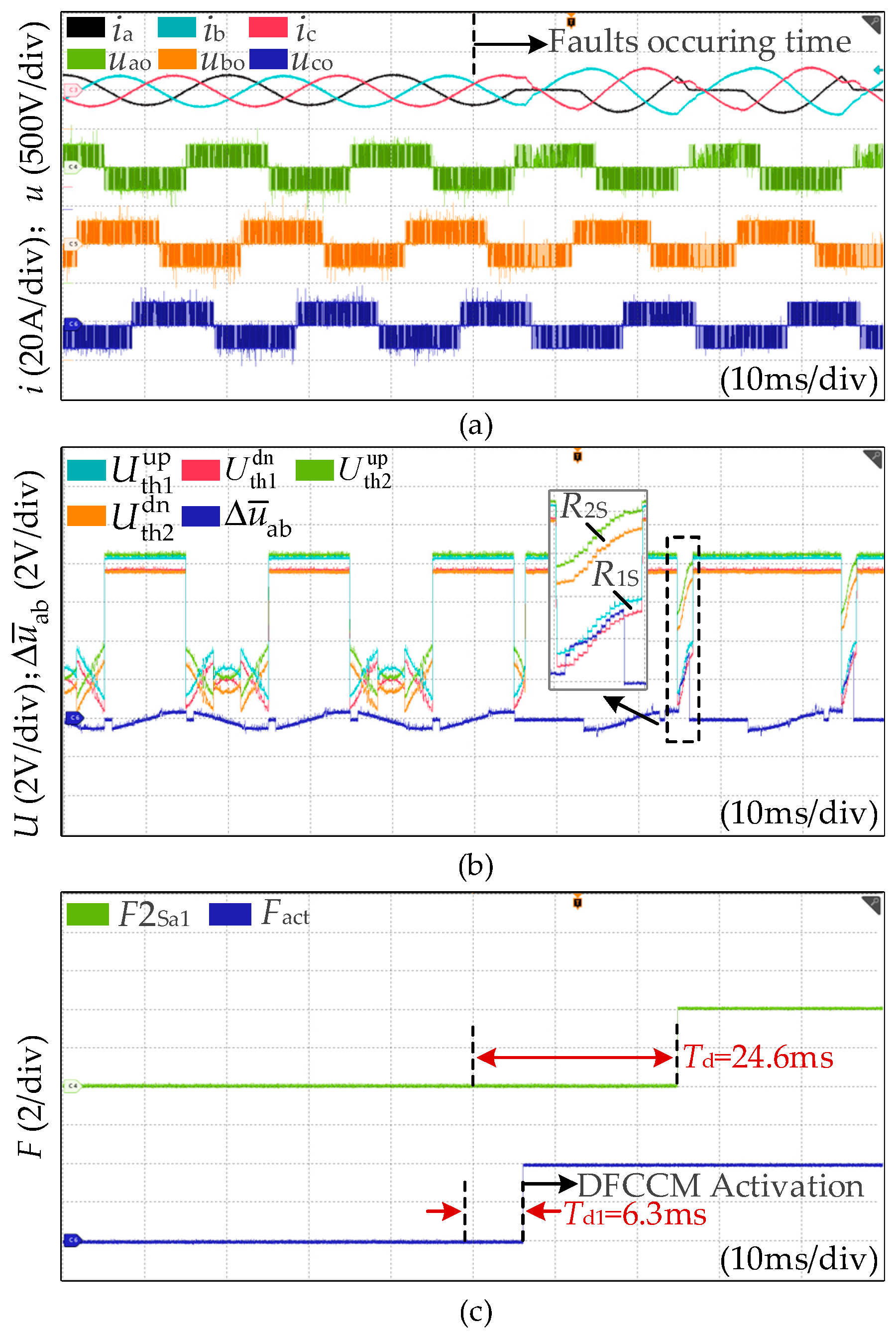
Case 4: The OC fault occurs at S_a1 when i_a < 0.

Figure 18 shows the experimental waveforms of case 4. In this condition, no liner current-decrease region is observed initially (Figure 18a). Once the FZR is detected, the DFCCM is activated. Following activation, a linear current-decrease region emerges, and the voltage residual $\Delta {\overline{u}}_{\mathrm{ab}}$ enters threshold region R_1S (Figure 18b), triggering the second-stage diagnostic variable F2_Sa1 to a logic high state (Figure 18c). According to the formulated fault location criterion, all the conditions for the fault location of switch S_a1 are satisfied. Consequently, S_a1 is determined to be the faulty switch.

The diagnosis results are summarized in

Table 3. Experiment results under cases 1–4.

Case No	Fault Type	Td1	Td	Identification Correctness
1	OC at Sa1, ia > 0	2.1 ms	14.7 ms	Yes
2	OC at Ma1, ia > 0	2.1 ms	14.6 ms	Yes
3	OC at Sa3, ia > 0	4.2 ms	14.7 ms	Yes
4	OC at Sa1, ia < 0	6.3 ms	24. 6 ms	Yes

Note: “T_d1” denotes time duration from fault occurrence to DFCCM activation (first-stage detection). “T_d” denotes time duration from fault occurrence to faulty switch identification.

As seen, the proposed method achieves accurate fault identification in all scenarios, with a full detection time within 25 ms. These results quantitatively demonstrate the responsiveness and correctness of the proposed diagnostic method.

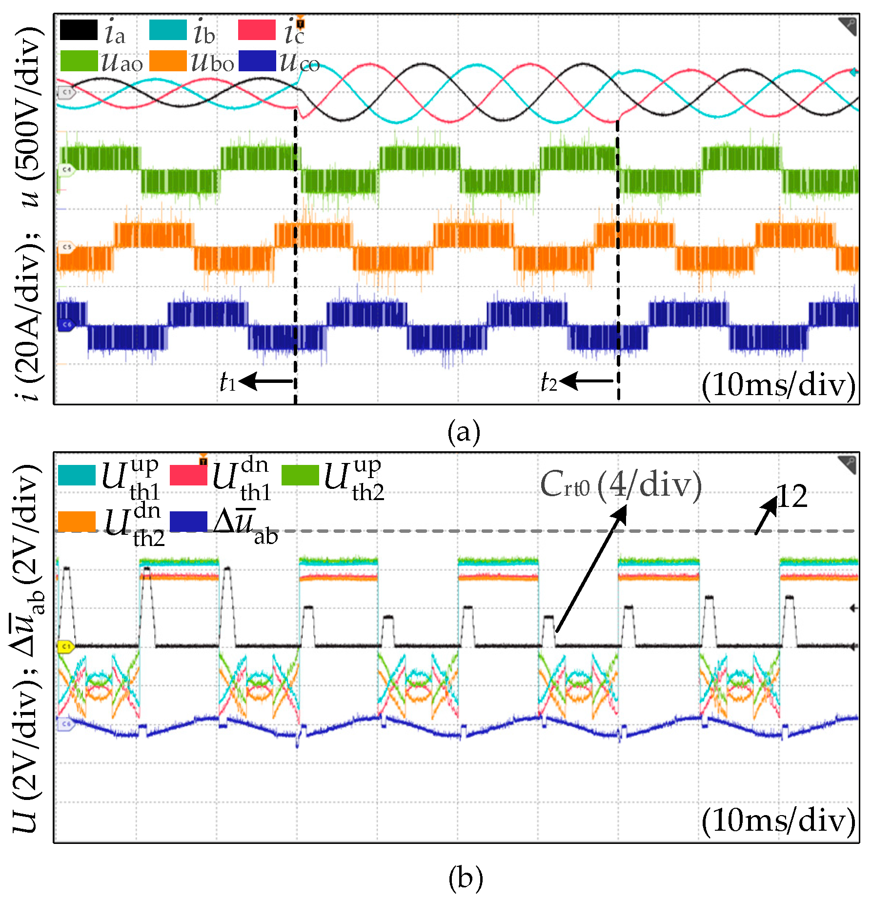
4.2. Robustness Verification of Proposed Method

To verify the robustness of the proposed fault diagnosis method, the experiments regarding the operation conditions of power variation and grid voltage fluctuation are carried out.

(1)

Case 5: Operation conditions of power variation

Figure 19 shows the experimental waveforms of case 5, where the reference power is step-increased at t₁ and step-decreased at t₂. It is observed that there is no FZR, and $\Delta {\overline{u}}_{\mathrm{ab}}$ does not enter the threshold regions under the operation conditions of power variation. Therefore, it will not cause misdiagnosis in case 5.

(2)

Case 6: Operation conditions of voltage fluctuation

Figure 20 shows the experimental waveforms of case 6, where the grid voltage sag happens at t_sag and returns to normal at t_nor. As seen, the output current of the converter is increased with constant power control during the grid voltage sag. Although the voltage residual $\Delta {\overline{u}}_{\mathrm{ab}}$ enters the threshold region R₁, there is no FZR. According to the formulated fault location criterion, the conditions of the switch fault location are not satisfied. Therefore, it will not cause misdiagnosis in case 6.

4.3. Comparison with Existing Method

The diagnosis time (DT), calculation burden (CB), diagnosis threshold type (DTT), and robustness are listed for the comparison, as shown in

Table 4. Comparison with exiting method.

Method	DT	CB (FLOPs)	DTT	Robustness
				OPF	GVF
[13]	<30 ms	<400	Fixed (Δ)	NO	NO
[14]	<15 ms	<400	Fixed (Δ)	NO	NO
[18]	<20 ms	<500	Fixed (Δ)	Yes	NO
[27]	<10 ms	>25,000	Fixed (Δ)	NO	NO
[28]	<20 ms	>25,000	Fixed (Δ)	NO	NO
[31]	<29.56 ms	>10,000	Fixed (Δ)	NO	NO
[32]	<54 ms	>10,000	Fixed (Δ)	NO	NO
Proposed	<25 ms	<350	Adaptive (▲)	Yes	Yes

Note: “DT” denotes diagnosis time. “CB” denotes calculation burden, which is quantified by the number of floating-point operations (FLOPs). “DTT” denotes diagnosis threshold type. “▲” denotes that the diagnosis threshold has an explicit physical model, while “Δ” denotes that the diagnosis threshold lacks a well-defined physical model. “OPF” denotes the output power fluctuation. “GVF” denotes the grid voltage fluctuation. The data of DT is derived from the experiment in corresponding reference. The date of CB is estimated based on algorithm structure described in corresponding reference.

. Both conventional CNN-based [27] and DNN-based [28] diagnostic methods can effectively identify faulty switches. However, their high calculation burden complexity (>25,000 FLOPs) limits real-time deployment on edge devices. To mitigate this, lightweight CNN models using TensorRT were introduced in [31,32], but still require high-performance platforms like NVIDIA Jetson, increasing system cost. In contrast, methods based on current vector trajectory [13,14] and current vector residuals [18] offer lower complexity, enabling DSP-based deployment. Yet, their reliance on fixed thresholds without physical models reduces robustness under power or voltage fluctuations. Although the proposed diagnostic method is not the most superior in terms of diagnostic time, it has some significant advantages, as follows: (1) It is non-AI-based and requires no data training, with an ultra-low calculation burden (<350 FLOPs), enabling low-cost real-time implementation. (2) It incorporates a two-stage voltage-based detection process that enhances accuracy and robustness under varying power and grid voltage conditions. (3) The diagnostic thresholds are derived from explicit physical models and adaptively tuned in real-time, achieving a balance between robustness and response speed.

5. Conclusions

In this article, the open-circuit fault diagnosis method using a generalized voltage residuals model and current polarity state is proposed to locate the faulty switch in a grid-tied HANPC converter. The approaches of current polarity state recognition and the generalized model of voltage residuals quantization are introduced in detail. Experimental results verify the effectiveness and accuracy of the proposed OC fault diagnosis method under typical operating conditions. The main conclusions are as follows.

(1) When different switches along the current path in the [P] or [N] states of the HANPC leg have OC faults, the output voltage and current characteristics of the faulty leg show very high similarity. For example, S_x1 and M_x1 share similar fault characteristics. It is the same for S_x4 and M_x2.

(2) The DFCCM is proposed to address the similarity in fault characteristics for switches at different positions. By reconfiguring the neutral-current path, the fault-current path is reconstructed and additional diagnostic information is obtained, enabling the identification of faulty switches with similar fault characteristics.

(3) The proposed quantization model of voltage residuals based on the variation of the pulse equivalent area is generalized. It can be extended to other types of inverters for the diagnosis of faulty switches, such as T-type converters and neutral-point-clamped converters.

Nevertheless, the proposed diagnosis method has certain limitations. Its robustness under extreme operating conditions, such as significant DC-link voltage fluctuations or strong background harmonics from the utility grid, has not been quantitatively validated and requires further investigation. Moreover, the proposed is primarily designed for single-switch fault scenarios, and its capability to identify simultaneous faults in multiple switches remains limited. Future research will focus on extending the method to address these challenges.

References

1. Shi, R.; Lan, C.; Dong, Z.; Yang, G. An Active Power Dynamic Oscillation Damping Method for the Grid-Forming Virtual Synchronous Generator Based on Energy Reshaping Mechanism. Energies 2023, 16, 7723. [Google Scholar] [CrossRef]
2. Wang, X.; Guo, Q.; Tu, C.; Che, L.; Xu, Z.; Xiao, F. A comprehensive control strategy for F-SOP considering three-phase imbalance and economic operation in ISLDN. IEEE Trans. Sustain. Energy 2025, 16, 149–159. [Google Scholar] [CrossRef]
3. Zhang, Y.; Li, K.; Zhang, L. Hybrid ANPC Grid-Tied Inverter Design with Passivity-Based Sliding Mode Control Strategy. Energies 2024, 17, 3655. [Google Scholar] [CrossRef]
4. Kim, Y.-J.; Kim, S.-M.; Lee, K.-B. Improving DC-link capacitor lifetime for three-level photovoltaic hybrid active NPC inverters in full modulation index range. IEEE Trans. Power Electron. 2021, 36, 5250–5261. [Google Scholar] [CrossRef]
5. Hakami, S.S.; Halabi, L.M.; Lee, K.-B. Dual-carrier-based PWM method for DC-link capacitor lifetime extension in three-level hybrid ANPC Inverters. IEEE Trans. Ind. Electron. 2023, 70, 3303–3314. [Google Scholar] [CrossRef]
6. Guo, Q.; Li, G.; Lin, J. A domain generalization network exploiting causal representations and non-causal representations for three-phase converter fault diagnosis. IEEE Trans. Instrum. Meas. 2024, 73, 2509713. [Google Scholar] [CrossRef]
7. Xiang, C.; Ouyang, Z.; Zhang, X.; Lu, H.H.C.; Cheng, S. An improved predictive current control of eight switch three-level post-fault inverter with common mode voltage reduction. IEEE Trans. Circuits Syst. I Regul. Pap. 2022, 69, 3861–3872. [Google Scholar] [CrossRef]
8. Xu, S.; Xu, X.; Du, H.; Wang, H.; Chai, Y.; Zheng, W.; Xhen, H. Comprehensive diagnosis strategy for power switch, grid-side current sensor, DC-link voltage sensor faults in single-phase three-level rectifiers. IEEE Trans. Circuits Syst. I Regul. Pap. 2024, 71, 3343–3356. [Google Scholar] [CrossRef]
9. Fan, C.; Xiahou, K.; Wang, L.; Wu, Q.H. Hybrid fault diagnosis of multiple open-circuit faults for cascaded H-bridge multilevel converter based on perturbation estimation convolution network. IEEE Trans. Instrum. Meas. 2024, 73, 3508812. [Google Scholar] [CrossRef]
10. Zhang, M.; Zhang, Z.; Li, Z.; Wang, J.; Zhang, Y.; Liu, S. A simple and effective open-circuit-fault diagnosis method for grid-tied power converters-A new technique based on tellegen’s theorem. IEEE J. Emerg. Sel. Top. Power Electron. 2023, 11, 2203–2213. [Google Scholar] [CrossRef]
11. Xu, S.; Sun, Z.; Yao, C.; Liu, K.; Ma, G. Open-switch fault-tolerant operation of T-type active neutral-point-clamped converter using level-shifted PWM. IEEE Trans. Circuits Syst. II Express Briefs 2021, 68, 2598–2602. [Google Scholar] [CrossRef]
12. Zhang, W.; He, Y. A simple open-circuit fault diagnosis method for grid-tied T-type three-level inverters with various power factors based on instantaneous current distortion. IEEE J. Emerg. Sel. Top. Power Electron. 2023, 11, 1071–1085. [Google Scholar] [CrossRef]
13. Kwon, B.H.; Kim, S.-H.; Kim, S.-M.; Lee, K.-B. Fault diagnosis of open-switch failure in a grid-connected three-level Si/SiC hybrid ANPC inverter. Electronics 2020, 9, 399. [Google Scholar] [CrossRef]
14. Kim, S.-H.; Kim, S.-M.; Park, S.; Lee, K.-B. Switch open-fault detection for a three-phase hybrid active neutral-point-clamped rectifier. Electronics 2020, 9, 1437. [Google Scholar] [CrossRef]
15. Wu, Z.; Zhao, J. Open-circuit fault diagnosis method for grid-connected bidirectional T-type converter based on geometrical similarity measurement. IEEE Trans. Power Electron. 2022, 37, 15571–15582. [Google Scholar] [CrossRef]
16. Zhang, M.; Zhang, Z.; Li, Z.; Chen, H.; Zhou, D. A unified open-circuit-fault diagnosis method for three-level neutral-point-clamped power converters. IEEE Trans. Power Electron. 2023, 38, 3834–3846. [Google Scholar] [CrossRef]
17. Xu, S.; Huang, W.; Wang, H.; Zheng, W.; Wang, J.; Chai, Y. A simultaneous diagnosis method for power switch and current sensor faults in grid-connected three-level NPC inverters. IEEE Trans. Power Electron. 2023, 38, 1104–1118. [Google Scholar] [CrossRef]
18. Li, G.; Xu, S.; Sun, Z.; Yao, C.; Ren, G.; Ma, G. Open-circuit fault diagnosis for three-level ANPC inverter based on predictive current vector residual. IEEE Trans. Ind. Appl. 2023, 59, 6837–6851. [Google Scholar] [CrossRef]
19. Wu, Z.; Zhao, J.; Luo, H.; Liu, Y. Real-time open-circuit fault diagnosis method for T-type rectifiers based on median current analysis. IEEE Trans. Power Electron. 2023, 38, 8956–8965. [Google Scholar] [CrossRef]
20. Liang, Y.; Wang, R.; Hu, B. Single-switch open-circuit diagnosis method based on average voltage vector for three-level T-type inverter. IEEE Trans. Power Electron. 2021, 36, 911–921. [Google Scholar] [CrossRef]
21. Caseiro, L.M.A.; Mendes, A.M.S. Real-time IGBT open-circuit fault diagnosis in three-level neutral-point-clamped voltage-source rectifiers based on instant voltage error. IEEE Trans. Ind. Electron. 2015, 62, 1669–1678. [Google Scholar] [CrossRef]
22. Chen, M.; He, Y. Multiple open-circuit fault diagnosis method in NPC rectifiers using fault injection strategy. IEEE Trans. Power Electron. 2022, 37, 8554–8571. [Google Scholar] [CrossRef]
23. Wang, B.; Li, Z.; Bai, Z.; Krein, P.T.; Ma, H. A voltage vector residual estimation method based on current path tracking for T-type inverter open-circuit fault diagnosis. IEEE Trans. Power Electron. 2021, 36, 13460–13477. [Google Scholar] [CrossRef]
24. Zhang, W.; He, Y. A hypothesis method for T-type three-level inverters open-circuit fault diagnosis based on output phase voltage model. IEEE Trans. Power Electron. 2022, 37, 9718–9732. [Google Scholar] [CrossRef]
25. Zhang, W.; He, Y.; Chen, J. A robust open-circuit fault diagnosis method for three-level T-type inverters based on phase voltage vector residual under modulation mode switching. IEEE Trans. Power Electron. 2023, 38, 5309–5322. [Google Scholar] [CrossRef]
26. Chen, M.; He, Y. Open-circuit fault diagnosis in NPC rectifiers using reference voltage deviation and incorporating fault-tolerant control. IEEE Trans. Power Electron. 2024, 39, 1514–1526. [Google Scholar] [CrossRef]
27. Kim, S.-H.; Yoo, D.-Y.; An, S.-W.; Park, Y.-S.; Lee, J.-W.; Lee, K.-B. Fault detection method using a convolution neural network for hybrid active neutral-point clamped inverters. IEEE Access 2020, 8, 140632–140642. [Google Scholar] [CrossRef]
28. Selvakumar, P.; Muthukumaran, G. An intelligent technique for fault detection and localization of three-level ANPC inverter with NP connection for electric vehicles. Adv. Eng. Softw. 2023, 176, 103354. [Google Scholar] [CrossRef]
29. Yuan, W.; Li, Z.; He, Y.; Cheng, R.; Lu, L.; Ruan, Y. Open-circuit fault diagnosis of NPC inverter based on improved 1-D CNN network. IEEE Trans. Instrum. Meas. 2022, 71, 3510711. [Google Scholar] [CrossRef]
30. Shen, H.; Tang, X.; Luo, Y.; Xie, F.; Shi, Z. Online open-circuit fault diagnosis for neutral point clamped inverter based on an improved convolutional neural network and sample amplification method under varying operating conditions. IEEE Trans. Instrum. Meas. 2024, 73, 3512612. [Google Scholar] [CrossRef]
31. Yao, C.; Xu, S.; Ren, G.; Wu, S.; Li, G.; Sun, Z. Online open-circuit fault diagnosis for ANPC inverters using edge-based lightweight two-dimensional CNN. IEEE Trans. Power Electron. 2024, 39, 3979–3984. [Google Scholar] [CrossRef]
32. Ma, G.; Yao, C.; Xu, S.; Ren, G.; Sun, Z.; Wu, S. Real-time diagnosis of multiple open-circuit faults in ANPC inverters based on lightweight deployment of edge 2D-CNN. IEEE Trans. Ind. Electron. 2025, 4, 1–12. [Google Scholar]
33. Peng, X.; Xiao, F.; Tu, C.; Wang, L. A fault-tolerant control for hybrid active neutral-point-clamped converters with shared redundant unit under multiswitch open-circuit fault. IEEE Trans. Ind. Electron. 2025, 72, 8550–8560. [Google Scholar] [CrossRef]
34. Li, Z.; Wang, B.; Ren, Y.; Wang, J.; Bai, Z.; Ma, H. L- and LCL-filtered grid-tied single-phase inverter transistor open-circuit fault diagnosis based on post-fault reconfiguration algorithms. IEEE Trans. Power Electron. 2019, 34, 10180–10192. [Google Scholar] [CrossRef]
Figure 1. Grid-tied circuit of HANPC converters.
Energies 18 03855 g001
Figure 2. Modulation of the HANPC converters. (a) Space vector distribution. (b) Vector synthesis in 60° g-h coordinated system. (c) Gate signal for switches.
Energies 18 03855 g002
Figure 3. Operation modes of the phase leg. (a) [P], iinvx > 0, mode 1. (b) [O], iinvx > 0, mode 2. (c) [N], iinvx > 0, mode 3. (d) [O], iinvx < 0, mode 4. (e) [P], iinvx < 0, mode 5. (f) [O+], iinvx < 0, mode 6. (g) [N], iinvx < 0, mode 7. (h) [O+], iinvx > 0, mode 8.
Energies 18 03855 g003
Figure 4. Switching modulation interval of HANPC converters under unit power factor operation.
Energies 18 03855 g004
Figure 5. Voltage and current of HANPC converters under OC fault at different switches. (a) OC fault at Sa1, ia > 0. (b) OC fault at Ma1, ia > 0. (c) OC fault at Sa3, ia > 0. (d) OC fault at Sa1, ia < 0. (e) OC fault at Ma1, ia < 0. (f) OC fault at Sa3, ia < 0.
Energies 18 03855 g005
Figure 6. The method of differentiated fault characteristic construction.
Energies 18 03855 g006
Figure 7. The waveforms of HANPC in cases of Sa1 and Ma1 fault, respectively.
Energies 18 03855 g007
Figure 8. The current waveform of HANPC in case of Sa3 fault.
Energies 18 03855 g008
Figure 9. Operation mode of HANPC converters under Sa1 fault and Ma1 fault, respectively. (a) Sa1 fault. (b) Ma1 fault.
Energies 18 03855 g009
Figure 10. Equivalent circuit of grid-tied HANPC converters.
Energies 18 03855 g010
Figure 11. The waveform of HANPC in case of Sa3 fault. (a) Output currents. (b) Voltage residuals and its threshold region.
Energies 18 03855 g011
Figure 12. Schematic diagram of current polarity recognition algorithm based on sliding window counting.
Energies 18 03855 g012
Figure 13. The flow chart of fault diagnosis.
Energies 18 03855 g013
Figure 14. Experimental prototype of grid-tied HANPC converters.
Energies 18 03855 g014
Figure 15. Experimental waveforms in case 1. (a) Output currents and voltages. (b) Voltage residual and its threshold region. (c) Logic variables for diagnosis. (d) Current-state counting in sliding window.
Energies 18 03855 g015
Figure 16. Experimental waveforms in case 2. (a) Output currents and voltages. (b) Voltage residual and its threshold regions. (c) Logic variables for diagnosis.
Energies 18 03855 g016
Figure 17. Experimental waveforms in case 3. (a) Output currents and voltages. (b) Voltage residual and its threshold regions. (c) Logic variables for diagnosis. (d) Current-state counting in sliding window.
Energies 18 03855 g017
Figure 18. Experimental waveforms in case 4. (a) Output currents and voltages. (b) Voltage residual and its threshold regions. (c) Logic variables for diagnosis.
Energies 18 03855 g018
Figure 19. Experimental waveforms in case 5. (a) Output currents and voltages. (b) Voltage residual and its threshold regions.
Energies 18 03855 g019
Figure 20. Experimental waveforms in case 6. (a) Output currents and voltages. (b) Voltage residual and its threshold regions.
Energies 18 03855 g020