State of Health Prediction for Lithium-Ion Batteries Based on Gated Temporal Network Assisted by Improved Grasshopper Optimization

Abstract

Accurate SOH prediction provides a reliable reference for lithium-ion battery maintenance. However, novel algorithms are still needed because few studies have considered the correlations between monitored parameters in Euclidean space and non-Euclidean space at different time points. To address this challenge, a novel gated-temporal network assisted by improved grasshopper optimization (IGOA-GGNN-TCN) is developed. In this model, features obtained from lithium-ion batteries are used to construct graph data based on cosine similarity. On this basis, the GGNN-TCN is employed to obtain the potential correlations between monitored parameters in Euclidean and non-Euclidean spaces. Furthermore, IGOA is introduced to overcome the issue of hyperparameter optimization for GGNN-TCN, improving the convergence speed and the local optimal problem. Competitive results on the Oxford dataset indicate that the SOH prediction performance of proposed IGOA-GGNN-TCN surpasses conventional methods, such as convolutional neural networks (CNNs) and gate recurrent unit (GRUs), achieving an R² value greater than 0.99. The experimental results demonstrate that the proposed IGOA-GGNN-TCN framework offers a novel and effective approach for state-of-health (SOH) estimation in lithium-ion batteries. By integrating improved grasshopper optimization (IGOA) with hybrid graph-temporal modeling, the method achieves superior prediction accuracy compared to conventional techniques, providing a promising tool for battery management systems in real-world applications.

1. Introduction

To ensure the safe and reliable operation of electric vehicles (EVs) and alleviated mileage anxiety caused by the degradation of on-board lithium-ion batteries, it is necessary to achieve reliable prediction of the state of health (SOH) for lithium-ion batteries [1,2]. This is essential for extending battery life and effectively managing the safety of EV power battery systems. As a typical interdisciplinary cooperation in lithium-ion batteries, SOH prediction can be divided into two categories: model-based approaches and data-driven approaches. Model-based approaches, such as equivalent circuit models [3] and Brownian motion models [4], are usually combined with Kalman filters or particle filters [5,6]. However, they rely on accurate physical modelling, which is challenging and often unattainable in practical engineering projects. In contrast, data-driven approaches have become a research hotspot due to the fast development of sensor technology, which provides the possibility of analyzing battery degradation data. Unlike model-based approaches, data-driven methods do not require exact physical models or prior knowledge [7]. In general, the data-driven approaches include machine learning and deep learning. Traditional machine learning methods such as support vector regression (SVR) [8], random forest [9], and Gaussian process regression (GPR) [10] require extracting features from the operational data of lithium-ion batteries and then building appropriate regressors. However, these methods depend on manual feature engineering, which limits the in-depth analysis of degradation information for lithium-ion batteries. Contrastingly, deep learning methods have garnered significant interest due to the ability to automatically acquire degradation characteristics [11].

At the present, various deep learning methods such as convolutional neural networks (CNNs) [12], recurrent unit networks (GRUs) [13], and their variants have been developed for the SOC and SOH prediction of lithium-ion batteries, allowing for the acquisition of time series features [14]. For example, Sun et al. [15] introduced a CNN to predict the impedance spectrum, in which the implicit information of the impedance spectrum is used to reflect the degradation state of lithium-ion batteries. In [16], Liu et al. developed a deep fusion transfer learning network (DFTN) consisting of CNNs to improve the SOH estimation in EVs. Ma et al. [17] utilized long-short-term memory networks (LSTMs) to extract temporal information from lithium-ion batteries. Previous studies have shown that the SOH prediction of lithium-ion batteries based on recurrent neural networks (RNNs) and their variants mainly focuses on capturing the time-dependence of degradation data. Although it is possible for CNNs to capture interdependencies between different parameters while capturing temporal degradation information, it generally leads to a significant increase in computational cost due to the increase in the depth of the network. As an alternative solution, the historical degradation information of lithium-ion batteries can be extracted with the help of dilated causal convolution in temporal convolutional networks (TCNs). Here, the receptive field of the convolutional kernel is increased dramatically, while the number of layers and parameters of the network are only slightly increased. Hence, TCNs have enhanced prediction ability compared with CNNs in SOH prediction task. Recently, the potential of TCNs has been noticed by researchers. For instance, Liu et al. [18] developed an estimation method combining multi-feature extraction with TCNs to achieve accurate SOH prediction for lithium-ion batteries. In addition, these studies are mainly devoted to the acquisition of degradation information in Euclidean spaces, ignoring topological information in non-Euclidean space. Indeed, the potential relationships in Euclidean spaces are often obtained in predefined order. This limitation restricts the ability to capture dynamic interdependencies between key battery parameters (e.g., voltage, current) across different time steps. Graph neural networks (GNNs) provide a promising solution by modeling topological relationships without relying on predefined sequential orders, as required in traditional methods [19,20]. Although GNNs have been successfully applied in domains such as traffic forecasting and materials science, their application to state-of-health (SOH) prediction for lithium-ion batteries remains underexplored.

For the complex degradation data in lithium-ion batteries, the impact of hyperparameters like learning rate and layers increases with network complexity. Hence, the most popular method of improving the performance of neural networks involves optimizing hyperparameters. Hyperparameter optimization is regarded as an integer programming problem [21]. In early studies, manual experience was the primary method used for traditional hyperparameter optimization, leading to problems such as falling into local optima and inefficiency. To solve this issue, several meta-heuristic optimization algorithms, such as genetic algorithm (GA) [22], alpine skiing optimization algorithm (ASO) [23], grey wolf optimization algorithm (GWO) [24], improved whale optimization algorithm (IWOA) [25], and artificial bee colony (ABC) [26], have been introduced to alleviate these problems. These optimization algorithms optimize the hyperparameters of the neural network, but they may cause problems such as local optima and premature maturation. Similar to these algorithms, the traditional grasshopper optimization algorithm (GOA) also exhibits uneven random initialization and poor development levels in later stages [27,28]. Therefore, in the hyperparameter search process, the global search capabilities of GOA need to be improved.

Thus, an improved SOH prediction method named gated-temporal network assisted by improved grasshopper optimization algorithm (IGOA-GGNN-TCN) is developed. The three major contributions are described below.

(1)

A graph structure is constructed to represent the degradation information of lithium-ion batteries, enabling extraction of the interdependence among parameters such as voltage and current in non-Euclidean space using a GGNN. Based on this, a TCN is used to obtain the temporal dependence of lithium-ion batteries during the degradation process in the Euclidean space, avoiding the manual feature engineering.

(2)

An improved grasshopper optimization algorithm (IGOA) is developed to achieve the hyperparameter optimization of the GGNN-TCN, in which an adaptive attenuation function is proposed to alleviate problems such as poor convergence and stagnation during the searching process.

(3)

A SOH prediction method is proposed based on the GGNN-TCN and the IGOA for complex degradation data of lithium-ion batteries. The experiments on the show that it has better predictive ability compared to traditional methods.

The remainder of this paper is as follows. The preliminary method and the proposed method are described in Section 2 and Section 3, respectively. In Section 4, the simulation results using different battery datasets are shown. Some conclusions are given in Section 5.

2. Preliminaries

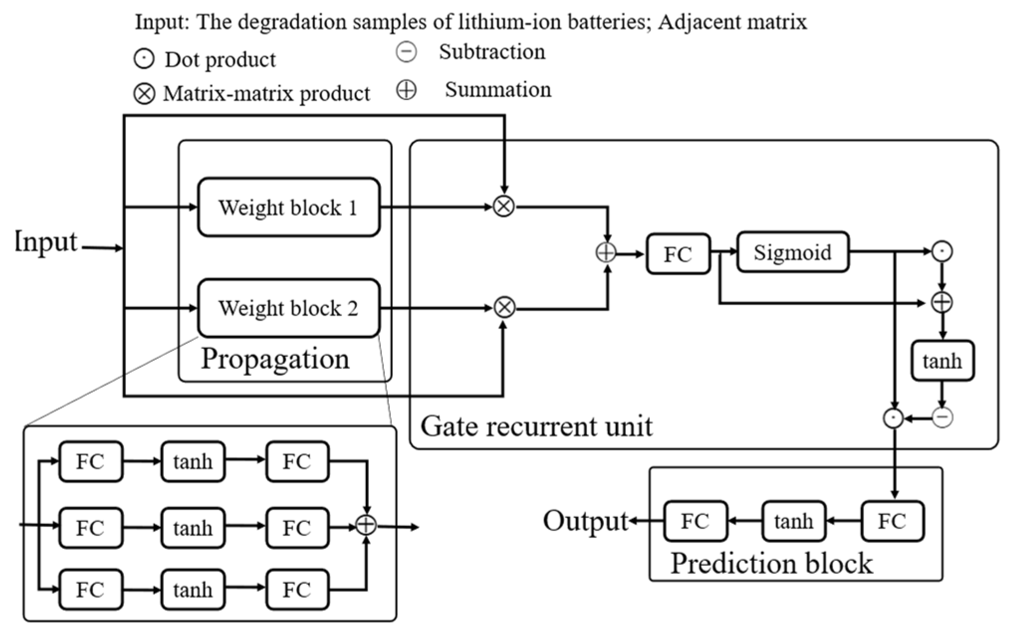
2.1. Gated Graph Convolution Network

The gated graph convolution network (GGNN) is considered a message-passing model based on GRU, which alleviates the limitations of GNNs in obtaining long-term degradation information of lithium-ion batteries [29]. Similar to GNNs, the degradation information can be given as follows:

$$G=(V,E,A)$$

(1)

where, V, E and A represent the nodes set, edge in the graph data, and adjacency matrix, respectively.

Then, the G is used as the input for the GGNN. Notably, the components in the GGNN include a messaging module and prediction module. The former is utilized to propagate degradation potential relationships between nodes. The latter is applied to achieve the prediction of degradation information for lithium-ion batteries. The whole structure of the GGNN is shown in Figure 1. This figure shows that there are two FC layers in each of the weight blocks in the propagation block. Notably, GRU is employed to integrate the degradation information obtained using the transmission module. Such an approach is useful in selecting effective degradation information and capturing causal and sequential degradation information in lithium-ion batteries. The propagation block is expressed as follows:

$$h_v^0={[x_v^T,0]}^T$$

(2)

$$a_v^t=A_v^T{[h_1^{(t-1)T},\dots ,h_{\left|V\right|}^{(t-1)T}]}^T{W}_a+b$$

(3)

$$u^t=\sigma (W_u{a}^t+U_u{h}^{t-1}+O_u{g}^{t-1}+b_u)$$

(4)

$$r^t=\sigma (W_r{a}^t+U_r{h}^{t-1}+O_r{g}^{t-1}+b_r)$$

(5)

$$\widetilde{h^t}=\tanh (W_h{a}^t+U_h(r^t\odot h^{t-1})+O_h{g}^{t-1}+b_h)$$

(6)

$$h^t=\widetilde{h^t}\odot u^t+h^{t-1}\odot (1-u^t)$$

(7)

where, $a^t$, $A_v^T$, $h^{t-1}$, and $g^{t-1}$ denote the information representation of adjacent nodes through the edge, the symmetric normalized adjacency matrix, the hidden state of the previous moment, and the global message for the previous moment, respectively. In addition, $u^t$ and $r^t$ represent the update gate and reset gate, respectively, and $h^t$ and $\widetilde{h^t}$ are the updated hidden state and the candidate hidden state, respectively. $W_x$, $U_x$,$O_x$, and $b_x$ are the trainable weights and biases. $\sigma$ and $\tanh$ denote the sigmoid and the tanh activation function, respectively.

For the prediction block, the graph output of degradation information can be defined as follows:

$$h^t=\widetilde{h^t}\odot u^t+h^{t-1}\odot (1-u^t)$$

(8)

where the correlation between adjacent nodes and the current node is determined by the sigmoid function $\sigma (*)$. $f_1$ and $f_2$ are the full connectivity layers.

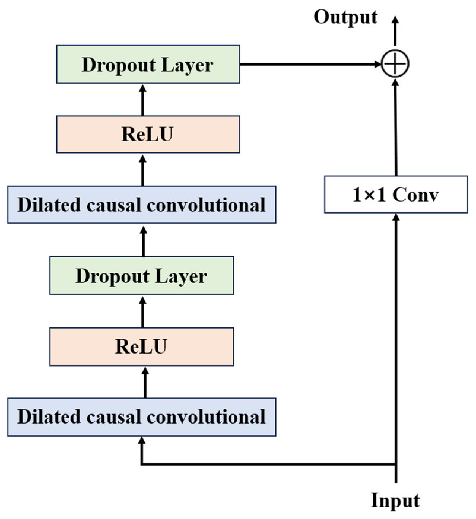
2.2. Temporal Convolutional Network

Based on the one-dimensional convolutional neural network, causal convolution, inflationary convolution, and residual linking are introduced. This approach alleviates the limitations of traditional CNNs in capturing the degradation information of long sequences, and the detail structure is shown in Figure 2. This figure shows that the TCN is composed of two small modules, each of which consists of 4 network layers, i.e., the inflated causal convolutional layer, the weight normalization layer (Weight-Norm), the activation function layer (ReLU), and the regularization layer (Dropout). In causal convolution, the predicted output at time t is obtained from the input data at time t and before time t. The advantage of this structure is that the output of the previous moment is not affected by the input of the next moment, allowing the model to satisfy the logical order of backward and forward dependencies when dealing with the SOH prediction tasks for lithium-ion batteries. In addition, dilation convolution is employed to ensure that more historical information is covered by the neural network while the model depth remains unchanged. This increases the ability of the TCN to extract information about the degradation of lithium-ion batteries. Although the ability of neural networks to extract degradation information from lithium-ion batteries improves as the number of layers increases, deeper network structures may cause problems such as gradient vanishing and gradient explosion. Thus, residual connectivity modules are introduced in TCNs, accelerating the process of feedback and convergence.

2.3. Grasshopper Optimization Algorithm

The grasshopper optimization algorithm (GOA) is a meta-heuristic optimization algorithm that was developed in 2017 and inspired by the hunting behavior of grasshoppers [30]. Similar to other meta-heuristic optimization algorithms, the GOA consists of both exploration and development phases. In the exploration phase, the grasshoppers can migrate long distances, which means that the algorithm can look for potentially high-quality solutions in a wide search space. In the development phase, grasshoppers move slowly and at a small pace, allowing the algorithm to perform small searches to speed up convergence. The algorithm is defined as follows:

$$X_i=S_i+G_i+A_i$$

(9)

where, $X_i$, $S_i$, $G_i$, and $A_i$ denote the position of the i-th grasshopper, social interactions among populations, the gravity force acting on the i-th grasshopper, and wind force on the i-th grasshopper, respectively.

$$S_i={\displaystyle \sum _{\begin{array}{l}j=1\\ j\ne i\end{array}}^{N}s(d_{ij})\widehat{d_l}}$$

(10)

$$d_{ij}=|x_j-x_i|$$

(11)

$$\widehat{d_{ij}}={\displaystyle \frac{x_j-x_i}{d_{ij}}}$$

(12)

$$s(r)=f{e}^{{\displaystyle \frac{-r}{l}}}-e^{-r}$$

(13)

where, $d_{ij}$ denotes the distance of the grasshoppers i and j from each other, $s(r)$ represents the functions of social relations, and f and l are the attraction strength and attraction scale, respectively.

$$G_i=-g\widehat{e_g}$$

(14)

$$A_i=u\widehat{e_{\omega }}$$

(15)

Here, g represents the gravitational constant, $\widehat{e_g}$ indicates a unit vector towards the center of the earth, and $\widehat{e_{\omega }}$ represents the unit vector of wind direction.

$$X_i^d=c\{{\displaystyle \sum _{\begin{array}{l}j=1\\ j\ne 1\end{array}}^{N}c\frac{u{b}_d-l{b}_d}{2}s(|x_j^d-x_i^d|)\frac{x_j-x_i}{d_{ij}}}\}+\widehat{T_d}$$

(16)

Here, d denotes the dimension of the variable; $x_i^d$ represents the optimal individual; $u{b}_d$ and $l{b}_d$ denote the upper and lower bounds of the variable, respectively; and $\widehat{T_d}$ is the optimal positions of individual grasshoppers. In addition c is the control parameter, which is given as follows:

$$c=c_{\max }-l{\displaystyle \frac{c_{\max }-c_{\min }}{L}}$$

(17)

where, $c_{\max }$ and $c_{\min }$ denote the max value and min value of the control parameter, respectively, and $l$ and $L$ represent the current iteration and the max iteration, respectively.

3. Proposed Method

3.1. Adjacency Matrix for GGNN

For the degradation data for lithium-ion batteries, V is expressed as follows:

$$Dis(x_i,x_j)=\left|\right|x_i-x_j|{|}^2=\left|\right|x_i|{|}^2+|\left|x_j\right|{|}^2-2\left|\right|x_i\left|\right|\times \left|\right|x_j\left|\right|\cos \theta$$

(18)

where $x_i,x_j$ denote the two different nodes, and the $\theta$ is the angle between $x_i,x_j$. Notably, the edges of one parameter are treated as the interactions from other parameters, while some represent disturbances during the degradation phase, and not all of them are be useful for SOH prediction. In this work, $x_i$ is regarded as a neighbor of $x_j$, if $\cos \theta$ > 0.2, as inspired by [31].

3.2. Improved Grasshopper Optimization Algorithm

Similar to other meta-heuristic optimization algorithms, the distribution of grasshopper populations is not uniform due to random initialization. These algorithms face problems such as falling into local optima and early maturation during the iterative process. To alleviate these problems, sine chaotic mapping and an improved adaptive fading strategy are developed to enhance exploration and exploratory ability.

First, sine is used for the initialization of the GOA, and the distributions of the generated sequences are more uniform [32]. The advantage of this method is that the sequences generated by sine have higher dynamic performance and more complex evolutionary trajectories. Thus, the diffusion performance is enhanced compared to the tent mapping method. The mathematical expression of sine is given as follows:

$$y_i^{j+1}={\displaystyle \frac{\delta \sin (\pi y_i^j)}{4}}$$

(19)

where, $y_i^j$ represents the j-th dimensional components of the i-th grasshopper after sine chaotic mapping. $\delta$ is limited to between 0 and 4. The chaotic state manifests when $\delta$ is greater than 3.8, and it becomes more obvious when $\delta$ is closer to 4. Therefore, $\delta$ is set to 4 in this paper. The initialization of $\delta$ can be redefined as follows:

$$z_i^j=l{b}_j+y_i^j\times (u{b}_j-l{b}_j)$$

(20)

In addition, an adaptive function is proposed to improve the exploitation and exploration capability of the GOA, and the function is assumed as follows:

$$S_p=2\gamma (\cos ({\displaystyle \frac{\pi t}{\sqrt{T^2+300}}})+1)$$

(21)

where, $\gamma$ is limited to [0.5, 1]. The new position update formula can be given as follows:

$$X_i^d=S_p\times c\{{\displaystyle \sum _{\begin{array}{l}j=1\\ j\ne 1\end{array}}^{N}c\frac{u{b}_d-l{b}_d}{2}s(|x_j^d-x_i^d|)\frac{(x_j-x_i)}{d_{ij}}}\}+\widehat{T_d}$$

(22)

In this paper, IGOA is used to achieve hyperparameter optimization of the proposed GGNN-TCN, which involves the learning rate, the number of neurons in the GGNN and TCN, and the batch size. Moreover, mean square error is used for the loss function, and the optimization processes for IGOA-GGNN-TCN are given in Figure 3. The details of IGOA-GGNN-TCN are described as follows.

First, considering the diversity of the input parameters and inconsistencies in their measurements, such as voltage, current, etc., the prediction performance would be limited if these data are fed into the GGNN-TCN. Therefore, min–max normalization is used for normalization of the input data, which is expressed as follows:

$$x_{norm}={\displaystyle \frac{x_i-x_{\min }}{x_{\max }-x_{\min }}}$$

(23)

where, $x_{norm}$, $x_i$, $x_{\max }$, and $x_{\min }$ denote the normalization of input data, raw data, and the maximum and minimum value of the raw data, respectively. Then, the IGOA is used for hyperparameter optimization of the proposed GGNN-TCN based on these normalization results. The details are defined as follows:

Step (1). The parameters of the IGOA, including the population G, number of grasshoppers N, and maximum iteration $\max t$, are initialized using the developed sine mapping method. Here, G is defined as follows:

$$G=[l{r}_i,n{g}_i,n{t}_i,b_i]$$

(24)

where, $l{r}_i$, $n{g}_i$, $n{t}_i$, and $b_i$ denote the learning rate, number of hidden neurons in the GGNN, number of hidden neurons in the TCN, and batch size in the i-th population, respectively.

Step (2). The fitness function and the -R² of the training set are calculated using the proposed GGNN-TCN. On this basis, the current optimal position is retained.

Step (3). The position of the grasshopper is updated according to Equation (22). Recalculating the -R² and replacing the result if the current result is better than the previous fitness value, otherwise retaining the previous position.

Step (4). If the $\max t$ is reached or the pre-requirement is satisfied, the optimal parameters and model are output. Otherwise, Steps (1)–(4) are executed again.

Step (5). The optimal parameters and GGNN-TCN are utilized for SOH prediction of lithium-ion batteries.

3.3. SOH Estimation Method for Lithium-Ion Batteries Based on IGOA-GGNN-TCN

In this section, a novel SOH estimation framework based on the proposed IGOA- GGNN-TCN method proposed in the previous section is described in detail, as shown in Figure 4. The proposed IGOA-GGNN-TCN includes three parts, including graph construction for input samples, acquisition of topological degradation relationships, and the optimization of hyperparameters for the GGNN-TCN. First, a fixed sliding time window is used to construct the input graph data. The window is set to 3, and the stride is defined as 1. On this basis, cosine similarity is used to calculate the weights for different nodes of different parameters. For the neural networks, which include a linear stacked structure of the GGNN and TCN, the predicted performance is affected by the learning rate, hidden layers, number of neurons, and batch size when the neural network structure is fixed. Therefore, the IGOA is developed to optimize the predicted performance of GGNN-TCN, improving the global search ability. Finally, the test dataset is used to validate the effectiveness of the optimized GGNN-TCN in SOH predictions.

4. Results and Discussion

4.1. Dataset Description

In this work, the Oxford ‘Path Dependence Battery Degradation Dataset’ is employed to validate the advancement of the proposed IGOA-GGNN-TCN method [31]. The Oxford Battery Degradation Dataset comprises eight small-format Kokam lithium-ion pouch cells (Cells 1–8), each with a nominal capacity of 740 mAh [32]. The experiments were conducted using a Bio-Logic MPG-205 battery tester under a controlled temperature of 40 °C, with a sampling interval of 1 s. The charging phase employed a constant current-constant voltage (CC-CV) protocol, whereas the discharging phase utilized the urban Artemis driving cycle. In the charging phase, the current is 0.74 A, and the charging cut-off voltage is 4.2 V, while discharge phase reduces voltage to 2.7 V at a constant cur-rent of 0.74 A. The system records voltage, current, temperature, and capacity data during both charging and discharging operations, with measurements taken every 100 cycles. In this dataset, the discharge condition of the aging test is closer to the dynamic operation condition of the real vehicle. This can more effectively verify the performance of the model under dynamic operation conditions. The current and voltage curves for the conducting capacity testing of batteries are shown in Figure 5a, and the discharge capacity decay curves of eight batteries are shown in Figure 5b.

The lithium-ion battery capacity exhibits progressive degradation with increasing charge–discharge cycles, showing varying rates of deterioration. To quantitatively characterize this capacity decay, we identify and extract multiple highly correlated features from both charging and discharging voltage profiles. During the charging phase, five representative parameters are obtained: the time interval (TI-ECVR) and charge capacity (CC-ECVR) between equal voltage rise points, along with the slope (SCVC), integral (ICVC), and peak temperature (MTCVC) of the charging curve. Similarly, the discharging process provides corresponding indicators including the time interval (TI-EDVD) and discharge capacity (DC-EDVD) between equal voltage drop points, supplemented by the discharge slope (SDVD), voltage integral (IDVC), and maximum temperature (MTDVC). These complementary feature sets comprehensively capture the battery’s aging characteristics through their representation of temporal dynamics, capacity–voltage relationships, energy transformation patterns, and thermal behavior during both operational phases.

As shown in Figure 6a, during the charging phase, TI-ECVR is Δt₁, V₁ is 3.4 V, and V₂ is 4.2 V. As shown in Figure 6b, during the discharging phase, TI-EDVD is Δt₂, V₃ is 4.1 V, and V₄ is 3.4 V. The calculation formulas for SCVC and SDVD in this article are as follows:

$$\left\{\begin{array}{l}{K}_1=\mathrm{\Delta }{t}_1/\left|V_2-V_1\right|\\ K_2=\mathrm{\Delta }{t}_2/\left|V_3-V_4\right|\end{array}\right.$$

(25)

where the parameters K₁ and K₂ represent the respective voltage curve gradients during the charging and discharging phases, Δt₁ and Δt₂ denote the corresponding temporal durations between these operational stages, V₁ and V₂ are the voltage values during the charging stage, and V₃ and V₄ are the voltage values during the discharging stage.

In addition, the incremental capacity (IC) curve refers to the curve of the current variation of a battery over time during the charging and discharging process. By analyzing the IC curve, important information about the charging and discharging characteristics, health status, and function of the battery can be obtained. This information can be used for applications such as fault diagnosis, capacity estimation, and life prediction of the battery.

This study focuses on characteristic features extracted from incremental capacity (IC) analysis to investigate battery degradation mechanisms. During the charging phase, we identify the IC peak (ICP) and its corresponding voltage position (ICPL) as key indicators, whereas the discharging phase reveals the IC valley (ICV) and its associated voltage location (ICVL) as equally significant markers. The IC curve itself is derived through numerical differentiation of the experimentally measured capacity-voltage (Q-V) profile, expressed mathematically as dQ/dV, where Q represents charge capacity and V denotes voltage. These distinctive IC curve features provide critical insights into phase transition behaviors and electrochemical degradation processes occurring within lithium-ion batteries. It is expressed as follows:

$${\displaystyle \frac{dQ}{dV}}\approx {\displaystyle \frac{I\cdot dt}{dV}}={\displaystyle \frac{\mathrm{\Delta }Q}{\mathrm{\Delta }V}}$$

(26)

where Q denotes the instantaneous charge/discharge capacity (Ah), and V represents the battery terminal voltage (V). The parameter I corresponds to the operating current (A), with t indicating the sampling timestamp. For numerical differentiation, we employ a fixed voltage increment ∆V of 5 mV, with ∆Q characterizing the corresponding capacity variation within this voltage window. This differential approach enables precise tracking of electrochemical state transitions during battery operation.

However, the original IC curve contains a large amount of noise, and the peak values on the IC curve are highly sensitive to noise, making it difficult to capture effective features for estimating battery capacity. In some studies, filters are used to denoise the original IC curve to achieve the expected smoothness. However, the type of filter and some of the related parameters introduce uncertainties to the final IC curve. Thus, this method is occasionally unable to effectively capture the corresponding peak and position information. Some studies have utilized the extended Kalman filter algorithm to filter IC curves and obtain smooth IC curves. Therefore, this article also uses the EKF algorithm to filter the IC curve, and the method is detailed in reference [33]. The system noise variance Q_EKF of the EKF algorithm in this article is 1 × 10⁻⁵, the measurement noise variance R_EKF is 10, and the prediction error covariance matrix P_EKF is 0.01. Figure 7 shows the results of filtering the IC curve using the EKF algorithm. From the graph, it can be seen that the IC curves for charging and discharging are very smooth, making it easy to extract the four features noted above.

Consequently, 14 features are described in this work and are coded as x0–x13. Some of the cosine similarity results for these batteries are shown in Figure 8. Here, the correlation of features differs at the same moment. According to the correlation guidelines, the correlation is very weak when the cosine similarity result is less than 0.2. Thus, correlations between features less than 0.2 are considered to have no edges between the two features when using these features to construct graph data.

4.2. Evaluation Metrics

The performance of the proposed method is evaluated using three widely used evaluation metrics, including R-square(R²), root mean square error (RMSE), and mean absolute percentage error (MAPE). These metrics are defined as follows:

$$R^2=1-{\displaystyle \frac{{\displaystyle \sum _{i=0}^n{(y_i-\widehat{y_i})}^2}}{{\displaystyle \sum _{i=0}^n{(y_i-\overline{y_i})}^2}}}$$

(27)

$$RMSE=\sqrt{{\displaystyle \frac{1}{n}}{\displaystyle \sum _{i=1}^n{(y_i-\widehat{y_i})}^2}}$$

(28)

$$MAPE={\displaystyle \frac{1}{n}}{\displaystyle \sum _{i=1}^n\left|\frac{y_i-\widehat{y_i}}{y_i}\right|}$$

(29)

where n denotes the total number of testing samples, and $\widehat{y_i}$, $y_i$, and $\overline{y_i}$ represent the predicted SOH values, the true SOH values and the mean SOH values, respectively. All methods used in this paper were implemented using Python 3.7 with the “torch_geometric 2.6.1” and “torch 2.5.1” libraries on Anaconda (Windows) running on a NVIDIA GTX 1060 Ti GPU, an Intel Core i7-6700 CPU, and 16 G of RAM. They are come from NVIDIA corporation and Intel corporation in Santa Clara, CA, USA.

4.3. Comparison Experiments Using Different Optimization Algorithms

To validate the optimization performance of the proposed IGOA in this work, the GOA, the subtraction-average-based optimizer (SABO) [34], symbiotic organisms search (SOS) [35], and war strategy optimization (WSO) [36] algorithms are adopted for comparison. The ranges of $G=[l{r}_i,n{g}_i,n{t}_i,b_i]$ are defined as $[0.001,0.01]$, $[16,128]$, $[16,128]$, and $[64,128]$, respectively. Notably, the maximum iteration for all the methods is set as 100, and the population size id defined as 5. The searching process is stopped when the optimization results do not change for 10 consecutive iterations. The predicted results of different methods are shown in Figure 9. This figure shows that the proposed IGOA can provide the optimal evaluation results for batteries. The detail evaluation results are listed in

Table 1. The comparison of different optimization algorithms for GGNN-TCN.

Methods	R2	RMSE	MAPE	Time (h)
IGOA-GGNN-TCN	0.9965	0.0027	0.0037	5.86 h
GOA-GGNN-TCN	0.9840	0.0059	0.0069	6.74 h
SABO-GGNN-TCN	0.9852	0.0057	0.0079	7.51 h
SOS-GGNN-TCN	0.9667	0.0086	0.0103	7.89 h

. GOA obtains the best results for the indexes R², MAPE, and computational time, while the RMSE provides the second-best results among the compared methods. The RMSE value of GOA is similar to that of SABO (0.059 > 0.057). Nevertheless, the MAPE, RMSE, R², and computational time are still improved by 46.3768%, 54.2373%, 0.2517% and 13.0563%, respectively. These experimental results indicate that the early-maturing issue and the balance of local optima and global optimum are improved in the GGNN-TCN.

4.4. Comparative Experiments of Different Deep Learning Methods

In this section, different structures are first introduced to verify the effectiveness of the proposed IGOA-GGNN-TCN, including TCN and GGNN. The predicted results are shown in Figure 1, and ablation experiment results are listed in

Table 2. The IGOA-GGNN-TCN ablation experiments.

Methods	R2	RMSE	MAPE
IGOA-GGNN-TCN	0.9965	0.0027	0.0037
TCN	0.9875	0.0052	0.0069
GGNN	0.9787	0.0069	0.0087

. Figure 10 shows that the IGOA-GGNN-TCN can provide accurate capacity results, demonstrating implicit relations from both Euclidean space and non-Euclidean space. In contrast, although GGNN and TCN also able to realize capacity prediction, graph neural networks or conventional neural networks only consider potential relationships in Euclidean space or non-Euclidean space. This limits their performance in predicting SOH in lithium-ion batteries.

Furthermore, different conventional methods, including stack CNN (sCNN), GRU, and LSTM [37], and advanced algorithms, including lightLA [38], CMGRU [39], MTGNN [40], AGCRN [41] and LAGCN [42], are used to validate the utility of the proposed IGOA-GGNN-TCN. The predicted SOH is visualized in Figure 11. The best prediction results can be obtained using IGOA-GGNN-TCN. The predicted error is shown in Figure 11b. The predicted error of IGOA-GGNN-TCN is minimal and stable compared with other methods. The details of the predicted evaluation metrics are listed in

Table 3. The prediction results of different deep learning methods.

Methods	R2	RMSE	MAPE
IGOA-GGNN-TCN	0.9965	0.0027	0.0037
sCNN	0.9635	0.0091	0.0106
GRU	0.9792	0.0068	0.0075
LSTM	0.9807	0.0066	0.0085
lightLA	0.9791	0.0068	0.0091
MTGNN	0.9815	0.0064	0.0068
AGCRN	0.9738	0.0076	0.0093
LAGCN	0.9835	0.0061	0.0051
CMGRU	0.9889	0.0049	0.0074

. Among the methods, CMGRU achieves the optimal evaluation results, i.e., R² is 0.9889, RMSE is 0.0049, and MAPE is 0.0074. In constant, these values are improved by 0.768%, 44.898%, and 50%, respectively, with IGOA-GGNN-TCN. This finding indicates that the predicted variance and the predicted bias can be guaranteed when using IGOA-GGNN-TCN. Thus, this method improves the SOH prediction precision for lithium-ion batteries. In addition, the training time and testing time of these methods were also obtained as listed in

Table 4. Training and testing times of different deep learning methods.

Methods	IGOA-GGNN-TCN	sCNN	GRU	LSTM	lightLA	MTGNN	AGCRN	LAGCN	CMGRU
Training time (s)	132.3445	104.0792	146.3712	153.2817	317.9561	141.5486	124.6817	135.8773	170.4817
Testing time (s)	0.02676	0.02201	0.02357	0.02618	0.04923	0.02596	0.02131	0.02816	0.02983

. Here, the training time of IGOA-GGNN-TCN is worse than the sCNN, GRU, LSTM, MTGNN, and AGCRN but better than lightLA, LAGCN and CMGRU. Indeed, the training process is offline, but this does not affect the actual engineering project. The training time can be improved with hardware improvements. The testing times for all the methods are less than 1 s, meeting the engineering requirements (10 s). Therefore, the proposed IGOA-GGNN-TCN method achieves competitive results.

5. Conclusions

To address the challenge of accurate SOH prediction when Euclidean and non-Euclidean spaces are considered, a novel gated temporal network assisted by improved grasshopper optimization (IGOA-GGNN-TCN) is developed based on the 14 features extracted from batteries in this work. In contrast to traditional methods, cosine similarity is adopted to describe the relationships among measured parameters obtained from the lithium-ion batteries, allowing for the potential relationships in non-Euclidean spaces to be captured using GGNN. Building on this foundation, TCN is employed to obtain potential relationships in the Euclidean space. In addition, considering that proper hyperparameters can effectively improve the prediction performance of GGNN-TCN—and that this is an integer programming problem—IGOA is proposed to enhance the prediction accuracy, accelerate the convergence speed, and reduce the tendency to fall into the local optima. Competitive experiment results on lithium-ion batteries demonstrate that the proposed IGOA-GGNN-TCN provides superior predictive performance, with an R² higher than 0.99 and an RMSE of 0.003. In the future, more batteries under different experimental conditions, including extreme conditions such as +2C (particle cracking) or low temperatures should be used to verify the effectiveness and sophistication of the proposed IGOA-GGNN-TCN.

References

1. Feng, X.; Zhang, Y.; Xiong, R.; Wang, C. Comprehensive performance comparison among different types of features in data-driven battery state of health estimation. Appl. Energy 2024, 369, 123555. [Google Scholar] [CrossRef]
2. Chen, Y.; Liu, Y.; He, Y.; Lyu, Z.; Cai, Y.; Zhang, S. SOC Estimation of Lithium-Ion Battery Pack Based on Discharge Stage Division and Fusion Modeling. IEEE Trans. Instrum. Meas. 2025, 74, 2515914. [Google Scholar] [CrossRef]
3. Li, C.; Yang, L.; Li, Q.; Zhang, Q.; Zhou, Z.; Meng, Y.; Zhao, X.; Wang, L.; Zhang, S.; Li, Y.; et al. SOH estimation method for lithium-ion batteries based on an improved equivalent circuit model via electrochemical impedance spectroscopy. J. Energy Storage 2024, 86, 111167. [Google Scholar] [CrossRef]
4. Long, Z.; Yuan, L.; Yin, A.; Zhou, J.; Song, L. A neural-driven stochastic degradation model for state-of-health estimation of lithium-ion battery. J. Energy Storage 2024, 79, 110248. [Google Scholar] [CrossRef]
5. Li, X.; Yuan, C.; Wang, Z.; He, J.; Yu, S. Lithium battery state-of-health estimation and remaining useful lifetime prediction based on non-parametric aging model and particle filter algorithm. Etransportation 2022, 11, 100156. [Google Scholar] [CrossRef]
6. Bracale, A.; De Falco, P.; Di Noia, L.P. Probabilistic state of health and remaining useful life prediction for Li-ion batteries. IEEE Trans. Ind. Appl. 2022, 59, 578–590. [Google Scholar] [CrossRef]
7. Zhou, J.; Qin, Y.; Luo, J.; Zhu, T. Remaining useful life prediction by distribution contact ratio health indicator and consolidated memory GRU. IEEE Trans. Ind. Inform. 2022, 19, 8472–8483. [Google Scholar] [CrossRef]
8. Wu, T.; Huang, Y.; Xu, Y.; Jiang, J.; Liu, S.; Li, Z. SOH prediction for lithium-ion battery based on improved support vector regression. Int. J. Green Energy 2023, 20, 227–236. [Google Scholar] [CrossRef]
9. Yang, N.; Song, Z.; Hofmann, H.; Sun, J. Robust State of Health estimation of lithium-ion batteries using convolutional neural network and random forest. J. Energy Storage 2022, 48, 103857. [Google Scholar] [CrossRef]
10. Jia, J.; Liang, J.; Shi, Y.; Wen, J.; Pang, X.; Zeng, J. SOH and RUL prediction of lithium-ion batteries based on Gaussian process regression with indirect health indicators. Energies 2020, 13, 375. [Google Scholar] [CrossRef]
11. Ma, Y.; Wang, Z.; Gao, J.; Chen, H. A novel method for remaining useful life of solid-state lithium-ion battery based on improved CNN and health indicators derivation. Mech. Syst. Signal Process. 2024, 220, 111646. [Google Scholar] [CrossRef]
12. Lee, G.; Kwon, D.; Lee, C. A convolutional neural network model for SOH estimation of Li-ion batteries with physical interpretability. Mech. Syst. Signal Process. 2023, 188, 110004. [Google Scholar] [CrossRef]
13. Zhang, C.; Luo, L.; Yang, Z.; Zhao, S.; He, Y.; Wang, X.; Wang, H. Battery SOH estimation method based on gradual decreasing current, double correlation analysis and GRU. Green Energy Intell. Transp. 2023, 2, 100108. [Google Scholar] [CrossRef]
14. Chen, Y.; Duan, W.; Huang, X.; Wang, S. Multi-output fusion SOC and SOE estimation algorithm based on deep network migration. Energy 2024, 308, 133032. [Google Scholar] [CrossRef]
15. Sun, Y.; Xiong, R.; Wang, C.; Tian, J.; Li, H. Deep neural network based battery impedance spectrum prediction using only impedance at characteristic frequencies. J. Power Sources 2023, 580, 233414. [Google Scholar] [CrossRef]
16. Liu, H.; Deng, Z.; Che, Y.; Xu, L.; Wang, B.; Wang, Z.; Xie, Y.; Hu, X. Big field data-driven battery pack health estimation for electric vehicles: A deep-fusion transfer learning approach. Mech. Syst. Signal Process. 2024, 218, 111585. [Google Scholar] [CrossRef]
17. Ma, Y.; Shan, C.; Gao, J.; Chen, H. A novel method for state of health estimation of lithium-ion batteries based on improved LSTM and health indicators extraction. Energy 2022, 251, 123973. [Google Scholar] [CrossRef]
18. Liu, S.; Chen, Z.; Yuan, L.; Xu, Z.; Jin, L.; Zhang, C. State of health estimation of lithium-ion batteries based on multi-feature extraction and temporal convolutional network. J. Energy Storage 2024, 75, 109658. [Google Scholar] [CrossRef]
19. Cheng, K.; Zhang, K.; Wang, Y.; Yang, C.; Li, J.; Wang, Y. Research on gas turbine health assessment method based on physical prior knowledge and spatial-temporal graph neural network. Appl. Energy 2024, 367, 123419. [Google Scholar] [CrossRef]
20. Wang, Z.; Yang, F.; Xu, Q.; Wang, Y.; Yan, H.; Xie, M. Capacity estimation of lithium-ion batteries based on data aggregation and feature fusion via graph neural network. Appl. Energy 2023, 336, 120808. [Google Scholar] [CrossRef]
21. Yeh, W.C.; Lin, Y.P.; Liang, Y.C.; Lai, C.; Huang, C. Simplified swarm optimization for hyperparameters of convolutional neural networks. Comput. Ind. Eng. 2023, 177, 109076. [Google Scholar] [CrossRef]
22. Ren, J.; Wang, Z.; Pang, Y.; Yuan, Y. Genetic algorithm-assisted an improved AdaBoost double-layer for oil temperature prediction of TBM. Adv. Eng. Inform. 2022, 52, 101563. [Google Scholar] [CrossRef]
23. Yuan, Y.; Yang, Q.; Ren, J.; Fan, J.; Shen, Q.; Wang, X.; Zhao, Y. Learning-imitation strategy-assisted alpine skiing optimization for the boom of offshore drilling platform. Ocean. Eng. 2023, 278, 114317. [Google Scholar] [CrossRef]
24. Yuan, Y.; Yang, Q.; Ren, J.; Mu, X.; Wang, Z.; Shen, Q.; Zhao, W. Attack-defense strategy assisted osprey optimization algorithm for PEMFC parameters identification. Renew. Energy 2024, 225, 120211. [Google Scholar] [CrossRef]
25. Duan, W.; Song, S.; Xiao, F.; Chen, Y.; Peng, S.; Song, C. Battery SOH estimation and RUL prediction framework based on variable forgetting factor online sequential extreme learning machine and particle filter. J. Energy Storage 2023, 65, 107322. [Google Scholar] [CrossRef]
26. Yuan, Y.; Shen, Q.; Xi, W.; Wang, S.; Ren, J.; Yu, J.; Yang, Q. Multidisciplinary design optimization of dynamic positioning system for semi-submersible platform. Ocean. Eng. 2023, 285, 115426. [Google Scholar] [CrossRef]
27. Meraihi, Y.; Gabis, A.B.; Mirjalili, S.; Ramdane-Cherif, A. Grasshopper optimization algorithm: Theory, variants, and applications. IEEE Access 2021, 9, 50001–50024. [Google Scholar] [CrossRef]
28. Hichem, H.; Elkamel, M.; Rafik, M.; Mesaaoud, M.T.; Ouahiba, C. A new binary grasshopper optimization algorithm for feature selection problem. J. King Saud Univ.-Comput. Inf. Sci. 2022, 34, 316–328. [Google Scholar] [CrossRef]
29. Tian, Z.; Li, X.; Chen, Z.; Zheng, Y.; Fan, H.; Li, Z.; Li, C.; Du, S. Interactive prostate MR image segmentation based on ConvLSTMs and GGNN. Neurocomputing 2021, 438, 84–93. [Google Scholar] [CrossRef]
30. Qin, P.; Hu, H.; Yang, Z. The improved grasshopper optimization algorithm and its applications. Sci. Rep. 2021, 11, 23733. [Google Scholar] [CrossRef] [PubMed]
31. Liang, P.; Li, Y.; Wang, B.; Yuan, X.; Zhang, L. Remaining useful life prediction via a deep adaptive transformer framework enhanced by graph attention network. Int. J. Fatigue 2023, 174, 107722. [Google Scholar] [CrossRef]
32. Birkl, C.R. Diagnosis and Prognosis of Degradation in Lithium-Ion Batteries. Ph.D. Thesis, University of Oxford, Oxford, UK, 2017. [Google Scholar]
33. Tian, J.; Xiong, R.; Shen, W. State-of-health estimation based on differential temperature for lithium ion batteries. IEEE Trans. Power Electron. 2020, 35, 10363–10373. [Google Scholar] [CrossRef]
34. Trojovský, P.; Dehghani, M. Subtraction-average-based optimizer: A new swarm-inspired metaheuristic algorithm for solving optimization problems. Biomimetics 2023, 8, 149. [Google Scholar] [CrossRef] [PubMed]
35. Cheng, M.Y.; Prayogo, D. Symbiotic organisms search: A new metaheuristic optimization algorithm. Comput. Struct. 2014, 139, 98–112. [Google Scholar] [CrossRef]
36. Ayyarao, T.S.L.V.; Ramakrishna, N.S.S.; Elavarasan, R.M.; Polumahanthi, N.; Rambabu, M.; Saini, G. War strategy optimization algorithm: A new effective metaheuristic algorithm for global optimization. IEEE Access 2022, 10, 25073–25105. [Google Scholar] [CrossRef]
37. Meng, X.; Sun, C.; Mei, J.; Tang, X.; Hasanien, H.M.; Jiang, J.; Fan, F.; Song, K. Fuel cell life prediction considering the recovery phenomenon of reversible voltage loss. J. Power Sources 2025, 625, 235634. [Google Scholar] [CrossRef]
38. Wang, Z.; Ma, Y.; Gao, J.; Chen, H. Remaining useful life prediction for solid-state lithium batteries based on spatial–temporal relations and neuronal ODE-assisted KAN. Reliab. Eng. Syst. Saf. 2025, 260, 111003. [Google Scholar] [CrossRef]
39. Wang, Z.; Ma, Y.; Gao, J.; Chen, H. Cured memory RUL prediction of solid-state batteries combined progressive-topologia fusion health indicators. IEEE Trans. Ind. Inform. 2025, 21, 4051–4060. [Google Scholar] [CrossRef]
40. Zheng, L.; Zhang, S.; Li, Y.; Liu, Y.; Ge, Q.; Gu, L.; Xie, Y.; Wang, X.; Ma, Y.; Liu, J.; et al. MTGNN: A drug–target–disease triplet association prediction model based on multimodal heterogeneous graph neural networks and direction-aware metapaths. J. Chem. Inf. Model. 2025, 65, 5921–5933. [Google Scholar] [CrossRef] [PubMed]
41. Gao, X.; Hu, Y.; Liu, S.; Yin, J.; Fan, K.; Yi, L. An AGCRN Algorithm for pressure prediction in an Ultra-long mining face in a medium–thick coal Seam in the Northern Shaanxi Area, China. Appl. Sci. 2023, 13, 11369. [Google Scholar] [CrossRef]
42. Han, H.; Zhu, R.; Liu, J.X.; Dai, L.Y. Predicting miRNA-disease associations via layer attention graph convolutional network model. BMC Med. Inform. Decis. Mak. 2022, 22, 69. [Google Scholar] [CrossRef] [PubMed]
Figure 1. The structure gated graph neural network, where FC is the fully connected layer.
Energies 18 03856 g001
Figure 2. The basic structure of the TCN.
Energies 18 03856 g002
Figure 3. The optimization process of SOH prediction based on IGOA-GGNN-TCN.
Energies 18 03856 g003
Figure 4. The framework of the IGOA-GGNN-TCN for SOH prediction of lithium-ion batteries.
Energies 18 03856 g004
Figure 5. Battery charging and discharging test experiments: (a) Current and voltage curves; (b) Battery capacity degradation curves.
Energies 18 03856 g005
Figure 6. Charge and discharge voltage curves: (a) charge curve, (b) discharge curve.
Energies 18 03856 g006
Figure 7. IC curve after the filtering processing: (a) charge curve, (b) discharge curve.
Energies 18 03856 g007
Figure 8. Correlation of different features at the same moment within a sliding window.
Energies 18 03856 g008
Figure 9. The prediction results of different optimization methods: (a) predicted capacity; (b) capacity error.
Energies 18 03856 g009
Figure 10. The prediction results of different structures: (a) predicted capacity; (b) capacity error.
Energies 18 03856 g010
Figure 11. The prediction results of different deep learning methods: (a) predicted capacity; (b) capacity error.
Energies 18 03856 g011