Practical Application of Complementary Regulation Strategy of Run-of-River Small Hydropower and Distributed Photovoltaic Based on Multi-Scale Copula-MPC Algorithm

Abstract

A novel multi-scale copula-based model predictive control (MPC) method is proposed to address the core regulation challenges of runoff hydropower and distributed photovoltaic systems within high-penetration renewable energy grids. Complex spatio-temporal complementarity under ecological constraints and the limitations of conventional methods were critically analyzed. The core innovation lies in integrating copula theory with MPC, enabling adaptive spatio-temporal optimization and weight adjustment to significantly enhance the efficiency of complementary regulation and overcome traditional performance bottlenecks. Key nonlinear dependencies of water–solar resources were investigated, and mainstream techniques (copula analysis, MPC, rolling optimization, adaptive weighting) were evaluated for their applicability. Future directions for improving modeling precision and intelligent adaptive control are outlined.

1. Introduction

Under the dual drivers of accelerated global climate governance restructuring and profound transformation of energy systems [1,2,3], the establishment of renewable energy-dominated power systems has been recognized as a strategic imperative for achieving carbon neutrality targets. China, positioned as the world’s largest renewable energy investor, has witnessed the formation of a distinctive “dual-core” energy configuration comprising run-of-river hydropower and distributed photovoltaics in remote mountainous and off-grid regions. Statistical records indicate that by 2024, these two energy sources collectively accounted for over 65% of the regional power supply in western China’s remote areas, achieving annual emission reductions equivalent to 120 million tons of standard coal combustion. However, in high-penetration renewable microgrid systems, the intermittency of photovoltaic generation and seasonal hydropower fluctuations have been observed to exhibit compounding effects, resulting in maximum system frequency deviations of ±1.2 Hz and 8–12% reductions in voltage compliance rates compared with conventional grids. This spatiotemporal heterogeneity in energy variability has rendered traditional deterministic control methodologies increasingly inadequate, necessitating the development of probabilistic-adaptive regulation frameworks. From an energy physics perspective, run-of-river hydropower and distributed photovoltaics demonstrate pronounced multi-timescale complementarity [4]. Photovoltaic output variability is characterized by diurnal fluctuations aligned with solar irradiance profiles, exhibiting peak hourly volatility rates of 70%/h. Conversely, run-of-river hydropower is constrained by base flow limitations, with diurnal regulation capacity typically restricted to 20–40% of rated output [5]. Seasonal-scale analysis reveals inherent counter-cyclic compensation: during wet seasons (May–October), hydropower availability escalates to 85%/h while photovoltaic efficiency declines by approximately 30% due to cloud cover [6]; during dry seasons (November–April), photovoltaic performance recovers to 92% of design capacity whereas hydropower output is reduced to 40–60% of installed capacity [7,8]. Although this cross-temporal complementarity provides physical foundations for coordinated control [9], current research remains predominantly confined to single-timescale analyses. Critical limitations persist in quantifying nonlinear hydro-meteorological couplings [10], where traditional linear correlation models have been shown to underestimate tail dependencies in precipitation-radiation joint distributions by up to 28%, significantly compromising system robustness under extreme weather conditions.

Current research in renewable energy complementarity exhibits distinct technical pathway differentiation [11]. In wind–photovoltaic hybrid systems, a robust theoretical framework has been established through extensive scholarly efforts [12], encompassing stochastic optimization models based on cointegrated wind–solar output and spatial smoothing quantification methods accounting for geographical dispersion [13]. Conversely, investigations into hydro-wind complementary systems have been predominantly focused on dynamic matching between reservoir regulation capacity and wind power fluctuations, yielding various Markov decision process-based optimization algorithms [14].

However, significant theoretical gaps are identified in existing studies targeting the specific combination of run-of-river hydropower and photovoltaics [15]. First, the absence of regulatory storage capacity in run-of-river systems has been systematically overlooked, with reservoir-based control models being inappropriately applied, resulting in a 42–68% failure rate for coordination strategies in field implementations [16]. Secondly, the coupling mechanisms between agricultural irrigation demands, ecological flow constraints, and energy regulation have not been systematically analyzed, particularly their compound effects on daily hydropower output variability (typically ranging 15–30%) [17]. thirdly, a multi-timescale modeling and control framework specifically tailored to this hybrid system has not been established–analysis of publications from 2015 to 2024 reveals that only 9% of relevant studies were found to address collaborative optimization beyond seasonal timescales. Finally, these theoretical deficiencies have been directly correlated with operational mismatches between control strategies and temporal resolution requirements. For instance, hourly-scale optimization schemes are frequently observed to neglect irrigation-induced hydraulic fluctuations, causing daytime power output deviations exceeding 12% of forecast values.

To address these challenges, a decade of theoretical advancements and technological breakthroughs in this domain is systematically reviewed in this study, with particular emphasis placed on the multi-scale copula–MPC methodology. A hierarchical spatiotemporal coupling framework is constructed, effectively resolving the theoretical limitations. This contribution not only provides novel methodological tools for stabilizing high-penetration renewable energy systems but also delivers critical insights for global off-grid energy transition practices.

The subsequent structure is organized as follows. Section 2 delves into multi-scale coupling mechanism analysis, Section 3 introduces and comparatively evaluates copula-based hydro-photovoltaic modeling theories, Section 4 optimizes the MPC-driven collaborative control framework, and Section 5 synthesizes key findings while proposing future research trajectories.

2. Multi-Scale Characteristics Analysis of Hydro–Photovoltaic Complementary Systems

2.1. Physico-Mathematical Modelling of Hydro-Photovoltaic Complementary Systems

The core of hydro-photovoltaic complementary systems lies in the coordinated operation of hydroelectric generating units and photovoltaic power generation units. As a critical component of hydropower stations, hydraulic turbines efficiently convert the hydrodynamic energy of rivers into mechanical energy. Establishing an accurate mathematical model of hydraulic turbines is essential for enhancing generator control performance and analyzing power system frequency stability. The flow rate, generated torque, and head height are key parameters characterizing their operational modes and dynamic behaviors. While turbines and penstocks are sometimes modeled as an integrated system, practical modeling faces challenges due to uncertainties in hydrological conditions and flow velocities.

Under minor disturbances such as slight grid load oscillations or fine adjustments of command signals, these variations induce subtle fluctuations in unit speed and other parameters. Since such changes remain within a controllable linear range, linear methods can effectively resolve the dynamic response of hydro-turbine governing systems. By integrating linear mathematical models of pressurized water supply systems [6], turbines, generators, and speed-governing control algorithms, a first-order linear differential equation model for hydro-turbine governing systems with single-penstock Francis turbines can be formulated under specific conditions, as shown in Equation (1).

$$\left\{\begin{array}{c}\dot{x}={\displaystyle \frac{1}{T_a+T_b}}\left(m_t-e_{n}x-m_g\right)\\ {\dot{m}}_t={\displaystyle \frac{1}{e_{qh}{T}_w}}\left[-m_t+e_{y}y-{\displaystyle \frac{e_m{e}_y{T}_w}{T_y}}(u-y)\right]\\ \dot{y}={\displaystyle \frac{1}{T_y}}(u-y)\end{array}\right.$$

(1)

The core of hydro-photovoltaic complementary systems resides in the synergistic operation between hydroelectric generating units and photovoltaic power generation units. As a critical component of hydropower stations, hydrodynamic energy contained in river flows is efficiently converted into mechanical energy by hydraulic turbines. Establishment of an accurate mathematical turbine model is essential for enhancing generator control and analyzing the frequency stability of power systems. Flow rate, generated torque, and hydraulic head are identified as key parameters characterizing operational modes and dynamic behaviors. In certain cases, turbines and penstocks are modeled as integrated systems; however, modeling efforts are challenged by uncertainties in hydrological conditions and flow velocities during practical implementation.

Under minor disturbances such as slight grid load oscillations or command signal adjustments, subtle fluctuations in unit speed and other parameters are induced. Since these variations remain within controllable linear ranges, linear methods can be employed to resolve the dynamic responses of hydro-turbine governing systems. Through integration of linear mathematical models for pressurized water conveyance systems, turbines, generators, and speed-governing control algorithms, a first-order linear differential equation model for Francis turbine governing systems with single-penstock configurations under specified conditions [6] is presented in Equation (2).

$$\left\{\begin{array}{c}\dot{\delta }={\omega }_{B}x\\ \dot{x}={\displaystyle \frac{1}{T_a}}\left(m_t-{\displaystyle \frac{E_q^{\prime }{V}_s}{X_{d\Sigma }^{\prime }}}\sin \delta -{\displaystyle \frac{V_s^2}{2}}{\displaystyle \frac{X_{d\Sigma }^{\prime }-X_{q\Sigma }}{X_{d\Sigma }^{\prime }{X}_{q\Sigma }}}\sin 2\delta -Dx\right)\\ {\dot{m}}_t={\displaystyle \frac{1}{e_{qh}{T}_w}}\left[-m_t+e_{y}y-{\displaystyle \frac{e_m{e}_y{T}_w}{T_y}}(u-y)\right]\\ \dot{y}={\displaystyle \frac{1}{T_y}}(u-y)\end{array}\right.$$

(2)

Selection of these parameters is based on the operational characteristics of typical small hydropower control systems. The unit inertia time constant T_a = 9.0 s reflects the relatively large rotational inertia characteristic of small hydropower control systems, which distinguishes hydroelectric units from thermal power units. The water inertia time constant T_w = 1.0 s characterizes the dynamic response of the hydraulic system, while the electro-hydraulic servo system time constant T_y = 0.1 s indicates the rapid response capability of modern governor systems. The transfer characteristics of small hydropower control systems are described by transfer coefficients in

Table 1. Fundamental Parameters of Run-of-River Small Hydropower Physical Model.

Parameter Symbol	Parameter Name	Value	Unit
wb	Base value of electrical angular velocity	314	rad/s
Ta	Unit inertia time constant	9.0	s
D	Damping coefficient	2.0	p.u.
Ed′	d-axis transient EMF (Note 1)	1.35	p.u.
Tw	Water inertia time constant	1.0	s
Ty	Electro-hydraulic servo system time constant	0.1	s
Xq	q-axis synchronous reactance	1.47	p.u.
Vs	System voltage	1.0	p.u.

, which represent linearized approximations of nonlinear relationships between output torque/flow rate and operating parameters near the working point.

In

Table 2. Parameters of Hydroelectric Unit Speed Control Systems.

Transfer Coefficient	Physical Meaning	Value
ex	Torque transfer coefficient w.r.t. rotational speed	−1.0
ey	Torque transfer coefficient w.r.t. guide vane opening	1.0
eh	Torque transfer coefficient w.r.t. hydraulic head	1.5
eqx	Flow transfer coefficient w.r.t. rotational speed	0
egy	Flow transfer coefficient w.r.t. guide vane opening	1.0
eqh	Flow transfer coefficient w.r.t. hydraulic head	1.0
em	Computational parameter (Note 1)	0.5

, a negative value of $e_x$ = −1.0 indicates that turbine output torque decreases with rotational speed increase, consistent with hydraulic turbine regulation characteristics. The coefficient e_y = 1.0 demonstrates a proportional relationship between guide vane opening and output torque. A value of $e_h=1.5$ reflects the strong influence of head variation on torque. The setting of flow transfer coefficient $e_{qx}=0$ simplifies model complexity, which is considered acceptable for engineering practices.

2.2. Data Sources and Preprocessing

In the operation and management of hydropower systems, the collection of relevant historical operational data is critical. Data sources primarily include multidimensional information such as meteorological data, hydrological observations, equipment operating status, and generated power [18]. These data are typically obtained through monitoring variables such as water station flow rate Q_t (m³/s), reservoir water level H_t (m), and P_hydro (kW). These variables not only support the real-time operation of power stations but also provide a foundation for subsequent analysis and decision-making. To enhance data comparability, the acquired multi-dimensional data must undergo per-unit normalization processing. Per-unit normalization eliminates the influence of differing dimensions and scales on model establishment, ensuring that all data are analyzed under a unified standard. The mathematical relationship of the flow data is expressed by Equation (3).

$$Q_{\mathrm{norm},t}={\displaystyle \frac{Q_t-Q_{\min }}{Q_{\max }-Q_{\min }}}$$

(3)

where Q_t is defined as the original runoff discharge at time step t, Q_min and Q_max represent the minimum and maximum runoff values recorded in the historical dataset, respectively. Following normalization, Q_norm,t ∈ [0, 1] is obtained, enabling cross-temporal comparative analysis of discharge data.

The distributed photovoltaic generation dataset is composed of irradiance G_t (W/m²), module temperature T_t (°C), and power output P_PV,t (kW). After outlier removal, the cleaned photovoltaic output P_PV,clean is expressed in Equation (4).

$$P_{\mathrm{PV}, \mathrm{clean} }=\left\{\begin{array}{ll}{P}_{\mathrm{PV},t}\hfill & \mathrm{if} \left|P_{\mathrm{PV},t}-{\widehat{P}}_{\mathrm{PV},t}\right|<3\sigma \hfill \\ {\widehat{P}}_{\mathrm{PV},t}\hfill & \mathrm{otherwise} \hfill \end{array}\right.$$

(4)

where P_PV,t (kW) denotes the original measured value of photovoltaic output power at time t, ${\widehat{P}}_{\mathrm{PV},t}$ (kW) represents the theoretically predicted value of photovoltaic output power at the same time interval. P_PVclean (kW) corresponds to the cleaned effective photovoltaic output power. The parameter $\sigma$ (kW) is defined as the standard deviation of photovoltaic output residuals, which quantifies the deviation between the actual photovoltaic system output power and its theoretically predicted value. This parameter serves as an indicator of system output stability and reliability. The parameter $\sigma$ is expressed in Equation (5).

$$\sigma =\sqrt{{\displaystyle \frac{1}{N}}{\displaystyle \sum _{t=1}^N{\left(P_{\mathrm{PV},t}-{\widehat{P}}_{\mathrm{PV},t}\right)}^2}}$$

(5)

The theoretically predicted value of photovoltaic output power at time t, denoted as ${\widehat{P}}_{\mathrm{PV},t}$, is expressed in Equation (6).

$${\widehat{P}}_{\mathrm{PV},t}=G_t\cdot \eta \cdot A\cdot \left[1-0.005\left(T_t-25\right)\right]$$

(6)

where G_t (W/m²) denotes the irradiance at time t, $\eta$ represents the module conversion efficiency (typical range: 15–22%), A (m²) is defined as the photovoltaic array area, and T_t (°C) corresponds to the module temperature. Outlier cleaning is recognized as a critical step for ensuring data quality and enhancing model prediction accuracy [19]. Primary anomaly identification is performed by evaluating deviations between measured and theoretical values, a methodology widely adopted for outlier removal [20]. Data points are retained only when their deviations fall within ±3σ of the theoretical predictions, as determined by predefined thresholds. This criterion aligns with the three-sigma principle (68-95-99.7 rule) of normal distributions, theoretically preserving 99.7% of valid data while minimizing accidental elimination [21]. Subsequently, a sliding window algorithm is implemented to dynamically adjust the cleaning process [22], enabling real-time adaptation to the dataset’s characteristics and external conditions for improved precision in anomaly detection.

Furthermore, an automated alert mechanism is activated when consecutive anomalies are detected, ensuring system stability and operational safety [23]. A multi-level verification protocol is employed, incorporating tiered thresholds to enhance responsiveness to potential anomalies [24]. In monitoring systems, persistent anomalies trigger alarms for further validation and mitigation, effectively reducing false-positive rates and improving alarm reliability [20]. Under adverse weather conditions (e.g., cloudy or rainy days), thresholds are adaptively relaxed to accommodate increased data variability, thereby avoiding erroneous classification of naturally fluctuating data as anomalies. This adaptive strategy not only refines data cleaning accuracy but also supports robust equipment maintenance and data validity in complex environmental scenarios.

2.3. Multi-Temporal Complementarity Characteristics of Hydro-Photovoltaic Systems

The hourly power fluctuation rate, denoted as ${\eta }_{1h}$ (%), is utilized to characterize the stochastic characteristics and fluctuation intensity of output power in electrical equipment or systems at an hourly temporal resolution [25]. This metric is designed to quantify short-term instability in power generation by analyzing deviations from a predefined baseline value and their dynamic evolution patterns within continuous time-series data, using a 1-h statistical window. Statistical methodologies and time-series analysis techniques are typically employed to calculate this indicator. Key parameters include srtandard deviation of fluctuation amplitudes, ange ratio (defined as the ratio of peak-to-valley difference to the mean value), skewness and kurtosis of probability density distribution functions, and frequency statistics of fluctuations derived from sliding window analysis. The hourly power fluctuation rate ${\eta }_{1h}$ (%) is mathematically expressed in Equation (7).

$${\eta }_{1h}={\displaystyle \frac{\left|P_{t+1}-P_t\right|}{P_{\mathrm{rated} }}}\times 100\%$$

(7)

where P_t (kW) denotes the power output at time t, with a valid range of 0 ≤ P_t ≤ P_rated, obtained through real-time monitoring. P_t+1 (kW) represents the power output at the subsequent time step, while P_rated (MW) corresponds to the rated capacity of the power plant, determined by equipment specifications. ${\eta }_{1h}$ (%) denotes the hourly power fluctuation rate, which typically ranges between 0–30% for photovoltaic systems and 0–10% for hydropower systems, calculated using Equation (7).

In the terms of the model, the hourly fluctuation rate can be characterized through autocorrelation functions to analyse temporal dependencies in power variations or via frequency–domain analysis to extract dominant fluctuation periods, thereby distinguishing between disturbances caused by abrupt load changes, intermittent renewable generation, and other factors [26]. From an application perspective, the hourly power fluctuation rate holds multifaceted significance in power systems planning and operation. First, in renewable energy integration assessments, the hourly fluctuation rates of photovoltaic and wind power systems directly influence the capacity configuration of voltage regulation devices and the optimization of dispatch strategies in distribution networks [27]. Second, regarding demand-side management, the hourly fluctuation characteristics of aggregated industrial and commercial loads serve as critical parameters for evaluating demand response potential, where the probability distribution morphology determines the types of flexible regulation resources required [28]. Furthermore, in electricity market mechanism design, hourly fluctuation rates are frequently incorporated as correction factors in locational marginal price models to reflect marginal cost variations induced by short-term power imbalances [29]. Notably, hourly fluctuation rates differ fundamentally from minute- and second-level metrics: Their temporal resolution captures intraday renewable generation trends while filtering high-frequency noise, making them essential inputs for day-ahead scheduling and intraday rolling adjustments [30].

Current research methodologies for hourly power fluctuation rate model exhibit interdisciplinary characteristics [31]. Probability box theory is employed to address interval estimation challenges under limited historical data conditions; copula functions effectively construct spatiotemporal correlation models for multi-energy system fluctuations; and deep learning-based frameworks [32], such as hybrid long short-term memory (LSTM) transformer networks, significantly enhance the extraction accuracy of cross-day fluctuation patterns [33]. With the advancement of power systems’ digitization, high-precision fluctuation rate prediction has emerged as a critical enabler for virtual power plant aggregation optimization and dynamic threshold control of energy storage systems.

Empirical studies demonstrate that photovoltaic systems exhibit an hourly power fluctuation rate (${\eta }_{1h}^{\mathrm{PV}}$) of up to 15%, whereas hydropower systems show a significantly lower rate (${\eta }_{1h}^{\mathrm{hydro}}$) of 5%. To quantify the composite fluctuation characteristics of hybrid photovoltaic-hydropower systems, a comprehensive fluctuation index ${\eta }_{\mathrm{sys}}$ (%) is expressed in Equation (8).

$${\eta }_{\mathrm{sys}}=\sqrt{{\left({\eta }_{1h}^{\mathrm{PV}}\right)}^2+{\left({\eta }_{1h}^{\mathrm{hydro}}\right)}^2}$$

(8)

The comprehensive fluctuation index ${\eta }_{\mathrm{sys}}$, expressed through a root mean square (RMS) operation to integrate the fluctuation contributions of both power sources, reflects the superimposed characteristics of the total system fluctuation rate. Due to the significantly higher volatility of photovoltaic output compared with hydropower, the value of ${\eta }_{\mathrm{sys}}$ is predominantly governed by photovoltaic fluctuations. However, the inherent low variability of hydropower generation partially mitigates system-wide fluctuations, thereby enhancing operational stability in hybrid systems.

To further evaluate the complementary characteristics between photovoltaic and hydropower systems at a daily temporal scale, a daily complementarity index C_daily is expressed in Equation (9).

$$C_{\mathrm{daily}}=1-{\displaystyle \frac{{\displaystyle \sum _{t=1}^{24}\left|P_{\mathrm{hydro},t}-P_{\mathrm{PV},t}\right|}}{2{\displaystyle \sum _{t=1}^{24}{P}_{\mathrm{PV},t}}}}$$

(9)

where P_hydro,t and P_PV,t denote the hydropower and photovoltaic power outputs (kW) at the t-th hour, respectively. The numerator is calculated as the sum of absolute hourly power differences between the two sources, while the denominator corresponds to twice the total daily photovoltaic power output. When the power curves of photovoltaic and hydro-power systems exhibit perfect complementarity (i.e., hydro-power output peaks compensate for photovoltaic output troughs), the numerator approaches zero, resulting in C_daily converging to 1, which indicates ideal complementarity. Conversely, if their output curves exhibit significant temporal overlap, the numerator increases, driving C_daily toward 0 and reflecting poor complementarity. This normalized metric objectively quantifies the temporal matching degree of the two power sources through dimensionless scaling, thereby providing a theoretical foundation for capacity allocation and dispatch optimization in hybrid systems.

Finally, the seasonal complementarity difference coefficient k, designed to evaluate the photovoltaic–hydropower complementary characteristics across seasonal wet-dry cycles, k is expressed in Equation (10).

$$\kappa ={\displaystyle \frac{P_{\mathrm{wet}}-P_{\mathrm{dry}}}{P_{\mathrm{annual}}}}$$

(10)

where P_wet (kW) denotes the average wet-season power output, typically spanning June–September, with typical wet-season output values ranging from 200 to 800 kW, calculated using the ${\displaystyle \frac{1}{n}}{\displaystyle \sum _{t\in T_{\mathrm{wet}}}{P}_t}$ (kW) methodology. P_dry represents the average dry-season power output, generally covering December–March, where output values are observed between 50 and 300 kW, derived via the ${\displaystyle \frac{1}{m}}{\displaystyle \sum _{t\in T_{\mathrm{dry}}}{P}_t}$ (kW) calculation method. P_annual corresponds to the annual average power output, which for this hydropower plant ranges from 50 to 300 kW, computed using the ${\displaystyle \frac{1}{8760}}{\displaystyle \sum _{t=1}^{8760}{P}_t}$ method. The seasonal wet–dry complementarity difference coefficient κ typically ranges from −0.5 to 0.8 for this hydropower system and serves as a critical indicator for evaluating the seasonal complementarity between wet and dry periods.

2.4. Spatial-Temporal Complementary Characteristics of Hydro-Photovoltaic Systems

A comprehensive regulation benefit index $\beta$ for cascade hydropower stations is proposed to quantify the synergistic effects between regulation capacity and energy efficiency in hydropower cascades. This index is expressed in Equation (11).

$$\beta ={\displaystyle \frac{{\displaystyle \sum _{i=1}^n{\alpha }_i}{h}_i}{{\displaystyle \sum _{i=1}^n{h}_i}}}$$

(11)

where a_i represents the regulation coefficient of the i-th power station, reflecting its regulation capacity type (non-regulated, daily regulated, or annually regulated) with assigned values of 0, 0.6, and 1.0 respectively; h_i denotes the net water head (m); and n indicates the total number of cascade stations. The index $\beta$ ranges within [0, 1], where values approaching 1 indicate stronger integrated regulation capacity of the cascade system.

This evaluation methodology employs water head as the weighting factor to quantify regulation capacity per unit hydraulic energy. The weight design reflecting practical engineering characteristics follows the “high-head station dominated regulation” principle. The system achieves $\beta$ = 1 (ideal regulation state) when all a_i = 1, and $\beta$ = 0 (non-regulated state) when a_i = 0. Engineering practice demonstrates that systems with $\beta$ > 0.7 can support high-penetration photovoltaic grid integration, while those with $\beta$ < 0.3 require pumped storage or energy storage facilities to ensure grid stability. This index system effectively integrates theoretical models with practical engineering requirements, providing quantitative decision-making support for renewable energy power systems planning.

The spatial distribution diversity gain index (D_PV) of photovoltaic (PV) arrays is introduced to evaluate the output fluctuation smoothing effect in PV plant clusters, as expressed in Equation (12).

$$\left\{\begin{array}{c}{D}_{\mathrm{PV}}=1-{\displaystyle \frac{{\sigma }_{P_{\mathrm{PV}, \mathrm{total} }}}{{\displaystyle \sum _{i=1}^m{\sigma }_{P_{\mathrm{PV},i}}}}}\\ {\sigma }_{P_{\mathrm{PV}}}=\sqrt{{\displaystyle \frac{1}{T}}{\displaystyle \sum _{t=1}^T{\left(P_{\mathrm{PV},i,t}-{\mu }_i\right)}^2}}\\ P_{\mathrm{total} ,t}={\displaystyle \sum _{i=1}^m{P}_{\mathrm{PV},i,t}}\end{array}\right.$$

(12)

where ${\sigma }_{P_{\mathrm{PV},i}}$ (kW) denotes the standard deviation of power output from the i-th PV plant, ${\sigma }_{P_{\mathrm{PV},\mathrm{total}}}$ (kW) represents the standard deviation of the aggregated cluster output (kW), m indicates the number of PV plants (integer, e.g., m = 15 for a regional cluster), and ${\displaystyle \sum _{i=1}^m{\sigma }_{P_{\mathrm{PV},i}}}$ corresponds to the cumulative sum of individual output standard deviations. This equation quantifies the smoothing enhancement achieved through cluster configuration by comparing the aggregated fluctuation with the superposition of individual fluctuations.

A D_PV approaching 1 indicates significant asynchrony in output fluctuations among cluster members, where spatial distribution diversity effectively reduces total power volatility. Conversely, a D_PV approaching 0 suggests highly synchronized output patterns, reflecting weak cluster-level smoothing effects.

Operational thresholds are established as follows. For D_PV < 0.2, plant spacing should be increased or layout adjustments implemented to enhance spatial diversity. When D_PV > 0.5, the cluster demonstrates sufficient smoothing capability to mitigate grid-connected power fluctuations and improve grid stability.

This index provides theoretical support for PV cluster planning by quantifying the impact of spatial distribution on power volatility. Particularly in high-penetration renewable energy integration scenarios, its application alleviates grid stress caused by intermittent generation, thereby contributing to stable operation of the power system.

The hydro-photovoltaic spatial synergy matching index (M) is established to evaluate the geographic coordination of renewable energy resources, as expressed in Equation (13).

$$\left\{\begin{array}{c}M={\displaystyle \frac{{\displaystyle {\iint }_A{f}_{\mathrm{hydro}}}(x,y)\cdot f_{\mathrm{PV}}(x,y)dxdy}{\max \left(P_{\mathrm{hydro} },P_{\mathrm{PV}}\right)}}\\ P_{\mathrm{hydro}}={\displaystyle {\iint }_A{f}_{\mathrm{hydro} }}(x,y)dxdy\\ P_{\mathrm{PV}}={\displaystyle {\iint }_A{f}_{\mathrm{PV}}}(x,y)dxdy\end{array}\right.$$

(13)

where f_hydro(x,y) (kW/km²) represents the hydro-power spatial density function, derived through interpolation of hydro-logical station data, reflecting water energy potential per unit area. f_PV(x,y) (kW/km²) denotes the photovoltaic spatial density function, calculated by integrating solar irradiance GIS datasets with terrain slope analysis, which quantifies the joint development potential of both energy sources per unit area. A (km²) signifies the study area, defined as the geographic boundary-delimited integration domain. P_hydro and P_PV correspond to the total regional hydro-power and photovoltaic development potentials (kW), respectively, obtained through spatial integration of their density functions.

The index is normalized using max (P_hydro, P_PV) to eliminate scale disparities between energy sources, M ensuring dimensionless output within [0, 1]. A value of M = 1 indicates perfect spatial congruence between hydro-power and photovoltaic resources, signifying optimal synergy, while M→0 implies minimal coordination.

Classification criteria for the spatial synergy matching index M are systematically categorized in

Table 3. Grading Standards of the Hydro-PV Spatial Matching Index (M).

Grade	M Range	Development Strategy
High	0.7–1.0	Local consumption
Medium	0.4–0.7	Regional coordination required
Low	0–0.4	Long-distance transmission + energy storage integration

.

In engineering practice, as shown in Table 3, the grading standards of M provide direct guidance for planning decisions. When M > 0.7, this indicates significant spatial synergy between hydro and photovoltaic resources, and distributed PV systems should be prioritized to enhance complementary energy efficiency. Conversely, when M < 0.4, adjustments to hydro-power dispatch radius or the integration of energy storage facilities are required to mitigate spatial distribution disparities.

Analysis of

Table 4. Correlation Analysis Between the Hydro-PV Spatial Matching Index M and Other Metrics.

Metric	Relationship with M	Joint Analysis Application Scenarios
Daily Complementarity Cdaily	High M typically corresponds to high Cdaily	Prioritize regions with high M and Cdaily for development
Diversity DPV	High M may reduce DPV (geographical concentration)	Pareto optimality between M and DPV must be balanced
Regulation Benefit $\beta$	High $\beta$ regulation benefits can compensate for low M limitations	Cross-regional hydro-PV complementary system planning

reveals that the correlation between the hydro-photovoltaic spatial matching index M and daily complementarity C_daily reflects fundamental spatiotemporal synergy mechanisms in hybrid energy systems. A positive correlation is typically observed between high M and high C_daily, indicating that greater geographical overlap of hydro and photovoltaic resources enhances diurnal complementary benefits. The C_daily metric quantifies the temporal offset characteristics between photovoltaic daytime output and hydropower nighttime peak regulation, thereby providing critical parameters for system stability evaluation. When C_daily < 0.5, insufficient diurnal complementarity necessitates the integration of energy storage systems to mitigate power fluctuations. Under such conditions, regions with high M values are prioritized for energy storage deployment due to their spatial synergy advantages, effectively reducing transmission losses and improving overall energy efficiency. Further analysis demonstrates that in high-M regions, the geographical co-location of hydro and photovoltaic resources allows extended control cycles for model predictive control MPC, thereby reducing computational complexity. Conversely, in low-M regions, shortened MPC control cycles are required to address more frequent power fluctuations. This strategy, based on the joint analysis of M and C_daily, establishes a theoretical framework for real-time dispatch optimization in multi-energy systems.

3. Hydro-Photovoltaic Complementarity Modeling Based on Copula Probability Functions

3.1. Theoretical Framework of Copula Probability Functions

Copula theory is recognized as a pivotal tool for multivariate probabilistic modeling, with its significance deriving from the innovative decoupling of joint probability distribution structures [26]. Sklar’s theorem, proposed in 1959, fundamentally redefined statistical understanding of dependency mechanisms. Any n-dimensional joint distribution function F(x₁, …, x_n) can be decomposed into a composite structure comprising n marginal distribution functions F₁(x₁), …, F_n(x_n) and a copula function C; C is expressed in Equation (14).

$$\begin{array}{c}{F}_{X,Y}(x,y)=C\left(F_X(x),F_Y(y)\right)=C(u,v)\\ c(u,v)={\displaystyle \frac{{\partial }^{2}C(u,v)}{\partial u\partial v}}\end{array}$$

(14)

The copula function ${\left[0,1\right]}^n\to \left[0,1\right]$ is defined as F_X,Y(x,y), representing the joint cumulative distribution of hydro-power (X) and photovoltaic (Y) outputs. Here, F_X, F_Y denote the marginal distributions, where hydro-power outputs are typically modelled by Gamma distributions and photovoltaic outputs by Beta distributions. Key variables in the copula framework are summarized in

Table 5. Definitions of Core Variables in Copula equation.

Symbol	Mathematical Definition	Physical Interpretation	Constraints
FX,Y(x,y)	P(X ≤ x,Y ≤ y)	Joint cumulative distribution of hydro (X) and PV (Y) outputs	Monotonically increasing, right-continuous
FX(x), FY(y)	P(X ≤ x), P(Y ≤ y)	Marginal distributions (Gamma for hydro, Beta for PV)	FX(−∞) = 0
C(u,v)	$\begin{array}{c}{\left[0,1\right]}^2\to \left[0,1\right]\end{array}$	Copula framework, pure dependency structure, excluding marginal effects	C(u,0) = C(0,v) = 0
u,v	u = FX(x), v = FY	Uniform variables via probability integral transform	u,v ∈ [0, 1]
c(u,v)	${\displaystyle \frac{{\partial }^{2}C}{\partial u\partial v}}$	Copula density function quantifying dependency intensity	∬c(u,v)dudv = 1

.

The variable definitions for the core Copula probability function (Equation (12)) are further clarified in Table 5. F_X,Y(x,y) denotes the joint cumulative distribution of hydropower (X) and photovoltaic (Y) output, with the constraint that it is monotonically increasing and right-continuous. F_X(x) and F_Y(y) represent the marginal cumulative distributions (e.g., Gamma distribution for hydropower, Beta distribution for photovoltaics), subject to the constraint F_X(−∞) = 0. C(u,v) refers to the copula function, which describes the pure dependence structure after removing marginal effects, under the constraints C(u,0) = C(0,v) = 0. u and v are uniformly distributed variables obtained after probability integral transformation, constrained by u,v ∈ [0, 1]. c(u,v) indicates the copula density function, measuring dependence intensity at a specific point (u, v), with the constraint ∬c(u,v)dudv = 1.

Copula theory distinctly decouples marginal distribution characteristics from interdependency relationships, which are often conflated in conventional statistics, thereby providing a modular analytical framework for complex system model. Copula functions are categorized into four major classes: elliptical copulas (e.g., Gaussian, Student’s t), Archimedean copulas (e.g., Clayton, Gumbel), vine copulas, and hierarchical Kendall copulas.

Mathematically, a copula function C${\left[0,1\right]}^n\to \left[0,1\right]$ is a multivariate joint distribution function with uniform marginal distributions [27]. The existence of such functions is guaranteed by the probability integral transform theorem; for continuous random variables x_i, the transformed variables U_i = F_i (X_i) follows uniform distributions on [0, 1]. This transformation maps raw data to a standardized probability space, enabling dependency model independent of marginal distributions. This unique feature of copula theory has proven particularly advantageous in non-Gaussian energy data models. For instance, when modelling the leptokurtic distributions of renewable energy outputs, Student’s t-distributions can be selected for marginals while employing Gumbel copulas to capture asymmetric tail dependencies.

A corollary of Sklar’s theorem further emphasizes the copula model’s flexibility; the copula function is uniquely determined when marginal distributions are continuous [28]. This theoretical foundation supports a two-stage empirical modelling process. Marginal distribution optimization with Kernel density estimation or generalized autoregressive conditional heteroskedasticity (GARCH) models are applied to individual variables. Dependency structure characterization employs copula functions to model interdependencies. This divide-and-conquer strategy effectively circumvents the “curse of dimensionality” inherent in traditional joint distribution parameter estimation.

The synergistic operation mechanisms of hydro-photovoltaic systems are critical for renewable energy integration. Statistical modelling methods provide theoretical support for analysing multi-energy coupling relationships. A Gumbel–copula-based joint probability distribution model is expressed in Equation (15).

$$C(u,v;\theta )=\exp \left(-{\left[{(-\ln u)}^{\theta }+{(-\ln v)}^{\theta }\right]}^{1/\theta }\right)$$

(15)

The parameter θ is characterized by explicit physical significance, quantifying the dependency intensity between the two energy sources. When θ = 1, the copula function degenerates into an independent structure, indicating no correlation between photovoltaic output and hydropower regulation. As θ approaches infinity, the model represents perfect positive dependence, where fluctuations of both resources are fully synchronized. Parameter estimation based on empirical data from the Yunnan region yields θ ≈ 2.5, reflecting a significant yet incomplete positive dependence in the hydro-PV complementary system. This outcome is closely associated with regional climatic features and dispatch strategies. The midday photovoltaic output peak coincides with periods of abundant hydro-power regulation capacity, forming inherent spatiotemporal coupling characteristics. However, the synergy level remains suboptimal due to meteorological uncertainties and grid constraints.

The tail dependence coefficient ${\lambda }_u$ is introduced to quantify system risks under extreme scenarios; ${\lambda }_u$ is expressed in Equation (16).

$${\lambda }_u=\underset{q\to 1}{\lim }P(U>q\mid V>q)=2-2^{1/\theta }$$

(16)

When θ = 2.5, the calculated tail dependence coefficient ${\lambda }_u$ = 0.68, indicating a 68% probability of synchronized anomalies in photovoltaic output and hydropower regulation under extremely high-value conditions. This statistical characteristic holds significant engineering implications. If photovoltaic midday output exhibits abnormally high values, the probability of hydropower systems bearing additional regulation pressure exceeds predictions from conventional linear correlation models. Physically, this phenomenon arises from seasonal synchronization between watershed runoff and solar irradiance, and proactive response strategies implemented by dispatch centres during peak periods. Notably, Gumbel copula demonstrates substantially stronger upper-tail dependence than lower-tail dependence, necessitating differentiated contingency plans for power surplus risks.

In energy systems correlation models, copula functions have garnered significant attention due to their capability to flexibly capture nonlinear and tail dependence relationships between variables. A comparative analysis of five widely used copula functions and their applicability in hydro-photovoltaic (hydro-PV) complementarity studies is presented in

Table 6. Comparative Analysis of Common Copula Functions in Hydro-PV Complementarity Studies.

Type	Functional Form	Application Scenarios	Adaptability in Hydro-PV Studies
Gaussian	$C_{\Phi }(u,v;\rho )$	Symmetric linear dependence	★★☆☆☆
Student-t	$C_t(u,v;\rho ,\nu )$	Significant tail dependence	★★★☆☆
Gumbel	$e^{-{\left[{(-\ln u)}^{\theta }+{(-\ln v)}^{\theta }\right]}^{1/\theta }}$	Upper-tail dependence	★★★★★ (PV midday peaks)
Clayton	${\left(u^{-\theta }+v^{-\theta }-1\right)}^{-1/\theta }$	Lower-tail dependence	★★★★☆ (hydro-power dry seasons)
Frank	$-{\displaystyle \frac{1}{\theta }}\ln \left(1+{\displaystyle \frac{\left(e^{-\theta u}-1\right)\left(e^{-\theta v}-1\right)}{e^{-\theta }-1}}\right)$	Non-tail symmetric dependence	★★☆☆☆

.

Table 6 provides a comparative analysis of five commonly used copula functions, focusing on their characteristics and applicability in hydro-PV complementarity research. Key aspects include applicable scenarios and suitability scores for hydro-PV applications. Frank copula is applicable to scenarios exhibiting independence in extreme value regions with no tail dependence. Student-t copula, Gumbel copula, and Clayton copula are suited for scenarios characterized by strong dependence in extreme value regions and potentially asymmetric tail dependence characteristics. Gaussian copula is appropriate for scenarios requiring symmetric linear dependence structures. Based on hydro-PV suitability scores, copula functions are demonstrated to be more effective in scenarios with significant tail dependence. Detailed analysis follows.

As revealed by the comparative analysis in Table 6, the Gaussian copula. Based on multivariate normal distribution assumptions, this function is applicable to symmetric linear dependence scenarios. Its inability to characterize tail dependence results in limited adaptability (★★☆☆☆) for hydro-PV studies. Although computationally efficient, its fitting capability is notably weak under extreme conditions such as midday PV output peaks or hydro-power dry seasons. The Student-t copula function enhanced by the degrees-of-freedom parameter ν extends Gaussian copula properties to capture tail dependence phenomena, and this is particularly suited for datasets with symmetric tail correlations (e.g., financial returns). However, its moderate adaptability (★★★☆☆) in hydro-PV systems probably stems from its symmetric tail assumption, which conflicts with the inherent asymmetric tail dependencies prevalent in energy systems. Regarding asymmetric copulas (Gumbel/Clayton), in the Gumbel copula, the parameter θ strengthens upper-tail dependence, aligning with the abrupt midday PV output surges, hence achieving optimal adaptability (★★★★★) [29]. Its advantage lies in model joint probabilities of extremely high-value events, such as synchronized PV output and grid load peaks under clear-sky conditions. The Clayton copula emphasizes lower-tail dependence; this function effectively describes dependency structures in low-value regions. Its strong adaptability (★★★★☆) [30] arises from its capability to model correlations between reduced hydropower output and streamflow during dry seasons. The divergence between Gumbel and Clayton copulas reflects the heterogeneous requirements for “peak” versus “trough” scenarios in energy systems. The Frank copula, characterized by a complex functional form and uniform dependence without tail emphasis, is suitable for scenarios with weak overall correlations, such as PV–hydropower interactions during normal hydrological periods. Nevertheless, its limited adaptability (★★☆☆☆) [31] stems from inadequate extreme-event model capabilities, restricting its utility in tail risk analysis.

3.2. Comparative Analysis of Hydro-Photovoltaic Coupling Modeling Methods

The adoption of the Beta distribution as the marginal distribution for PV output model is analysed. The probability density function of the Beta distribution is expressed in Equation (17).

$$f\left(P_{\mathrm{PV}};\alpha ,\beta \right)={\displaystyle \frac{P_{\mathrm{PV}}^{\alpha -1}{\left(1-P_{\mathrm{PV}}\right)}^{\beta -1}}{B(\alpha ,\beta )}}, 0\le P_{\mathrm{PV}}\le 1$$

(17)

where the normalized photovoltaic output P_PV is scaled to the range [0, 1] via min–max normalization, representing the instantaneous output percentage relative to rated capacity. The shape parameters α and β govern the left-tail and right-tail morphology of the distribution, respectively. When α is small, elevated probability density in the left tail corresponds to scenarios with near-zero PV output, such as nighttime or extreme weather conditions. Conversely, reduced β values intensify right-tail probability density, indicative of full-capacity output under ideal irradiation conditions. This characteristic enables effective characterization of the volatility and bimodal features inherent in PV output fluctuations driven by environmental factors.

The Beta function serves as the normalization constant to ensure unit probability density integration, $B(\alpha ,\beta )$ is expressed in Equation (18).

$$B(\alpha ,\beta )={\displaystyle {\int }_0^1{t}^{\alpha -1}}{(1-t)}^{\beta -1}dt$$

(18)

From an engineering perspective, the values of parameters $\alpha$ and $\beta$ should be adjusted based on practical scenarios. For instance, in regions with stable solar irradiance, increasing $\beta$ can reduce the concentration of full-output probabilities, whereas in cloudy areas, decreasing $\alpha$ elevates the likelihood of low-output probabilities. This flexibility enables the Beta distribution to adapt to power generation model under diverse climatic conditions. Notably, the conventional Beta distribution exhibits a uni-modal shape when $\alpha$,$\beta$ > 1, while bimodal characteristics typically require $\alpha$,$\beta$ < 1, resulting in a U-shaped distribution with higher probabilities at the extremes and lower probabilities in the intermediate range. This property may reflect complex scenarios where PV output frequently transitions between extremes (e.g., zero or full output), such as in regions affected by intermittent cloud cover. However, the parameter selection for bimodal characteristics must be carefully validated. If historical data show concentrated output in intermediate ranges (e.g., partial shading or twilight periods), the distribution assumptions should be re-evaluated. Additionally, the model parameters $\alpha$ and $\beta$ should be calibrated using historical generation data, and distribution suitability must be confirmed through statistical testing (e.g., Kolmogorov–Smirnov (K-S) test). In engineering applications, hybrid distributions or non-parametric methods can further enhance model robustness. By adjusting shape parameters to regulate distribution morphology, Beta distribution-based PV output model effectively captures spatiotemporal variations in generation characteristics, providing theoretical support for probabilistic power flow calculations, energy storage configuration optimization, and risk assessment in power systems. Nevertheless, the realization of bimodal characteristics relies on specific parameter combinations, necessitating scenario-specific parameter calibration and model validation in practical implementations.

In PV output models, the Beta distribution serves as an effective tool for describing stochastic generation patterns due to its unique bimodal characteristics and parametric flexibility. When shape parameters satisfy $\alpha$ < 1 and $\beta$ < 1, the Beta distribution adopts a U-shaped bimodal form, where the left peak ($P_{pr}\to 0^{+}$) corresponds to low-output scenarios (e.g., nighttime or rainy weather), and the right peak ($P_{pr}\to 1^{-}$) represents full-output states (e.g., clear-sky midday). This property accurately characterizes the polarized behaviour of PV output influenced by environmental factors, such as diurnal cycles and cloud shading, exemplified by frequent transitions between zero and full output in regions with intermittent cloud cover. Independent modulation of $\alpha$ and $\beta$ enables precise control over left- and right-tail morphologies, endowing the model with high adaptability to real-world generation scenarios. As shown in

Table 7. Comparative analysis of probability density functions with alternative distributions.

Distribution Type	Applicable Scenarios	Limitations	Advantages of Beta Distribution
Normal	Symmetrical unimodal patterns	Failure to characterize zero-output clustering	Bimodal modeling and boundary clustering capabilities
Weibull	Unilateral distributions (right/left-skewed)	Limited capacity to fit clear-sky full-output characteristics	Flexible modulation of both distribution tails
Gaussian Mixture	Multimodal scenarios	Parameter redundancy increases overfitting	Bimodal representation with only two parameters

, compared to conventional distributions, such as normal distribution (incapable of describing zero-output clustering), Weibull distribution (ineffective in fitting full-output characteristics), and Gaussian mixture models (suffering from parameter redundancy), the Beta distribution achieves bimodal model with only two parameters. Furthermore, its support interval [0, 1] inherently aligns with the normalized range of PV output, ensuring both mathematical simplicity and physical interpretability.

As demonstrated in Table 7, the practical engineering value of the Beta distribution is further highlighted in parameter estimation case studies. For a PV plant under clear-sky conditions ($\alpha$ = 0.82, $\beta$ = 0.58), the output distribution exhibits distinct bimodal characteristics: Peak 1 (probability density at $P_{pr}$ < 0.1) and Peak 2 ($P_{pr}$ > 0.9) account for 34% and 41% probabilities, respectively, reflecting the combined effects of diurnal cycles and transient cloud cover. Under cloudy conditions ($\alpha$ = 1.15, $\beta$ = 1.32), increased parameter values result in uni-modal distribution, with outputs concentrated in the intermediate range (30–70%), indicating frequent irradiance fluctuations but rare extreme values. For rainy conditions ($\alpha$ = 2.10, $\beta$ = 0.95), the left peak probability drops sharply to 6%, while a weak right peak (3%) persists, suggesting low-output dominance with intermittent recovery potential. These parameterized outcomes directly inform energy storage configuration and dispatch strategies: clear-sky scenarios require preparedness for abrupt output changes, cloudy conditions necessitate optimized mid-range energy management, and rainy environments demand enhanced focus on system stability during prolonged low-output periods. Furthermore, the weather-dependent sensitivity of Beta distribution parameters enables dynamic adaptation to diverse climatic features, laying the foundation for output prediction and risk assessment.

Despite its advantages in PV modelling, the application of the Beta distribution requires scenario-specific optimization. First, parameter calibration must rely on historical data using methods such as maximum likelihood estimation (MLE), and distribution validity should be verified through statistical testing (e.g., Kolmogorov–Smirnov (K-S) test). Second, complex multi-modal scenarios (e.g., simultaneous haze and dust impacts) may necessitate hybrid Beta models or integration with non-parametric kernel density estimation to improve adaptability. Third, variations in output characteristics across temporal scales (minute-level vs. hour-level) require models with multi-resolution analysis capabilities. Future research should explore dynamic parameter adjustment mechanisms, where real-time meteorological data are utilized to update $\alpha$ and $\beta$, thereby enhance responsiveness to short-term weather fluctuations. In summary, the Beta distribution balances model complexity with physical interpretability, offering a robust theoretical framework for PV output uncertainty modelling and optimized operation of modern power systems.

4. MPC-Based Coordinated Hydro-Photovoltaic Regulation Framework

4.1. Overview of Model Predictive Control Theory

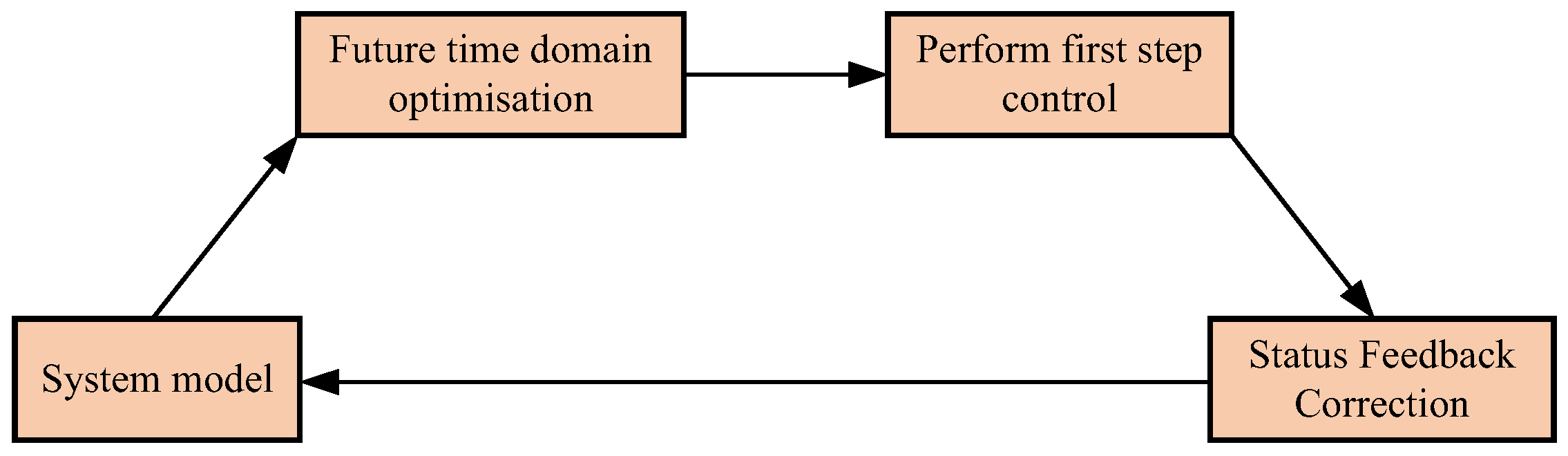
Model predictive control (MPC), also termed receding horizon control, dynamic matrix control, or generalized predictive control, is a feedback control strategy grounded in predictive models [32]. A rolling optimization approach is employed to approximate global optimality with local solutions, while feedback correction based on real-time system states ensures enhanced control performance, robustness, and stability. At each sampling instant, the future system states and outputs are predicted using the predictive model, and an open-loop optimal control problem over a finite horizon is solved. Subsequently, the predictive model is iteratively refined via feedback correction using actual system outputs, forming a closed-loop control optimization process. The first component of the derived optimal control sequence is then applied to the system. This optimization cycle is repeated at subsequent sampling instants, achieving continuous system regulation. As a feedforward-feedback composite control strategy based on dynamic models, MPC’s core mechanism lies in its ability to achieve optimal control under multi-objective constraints through online rolling optimization and closed-loop correction, as illustrated in Figure 1.

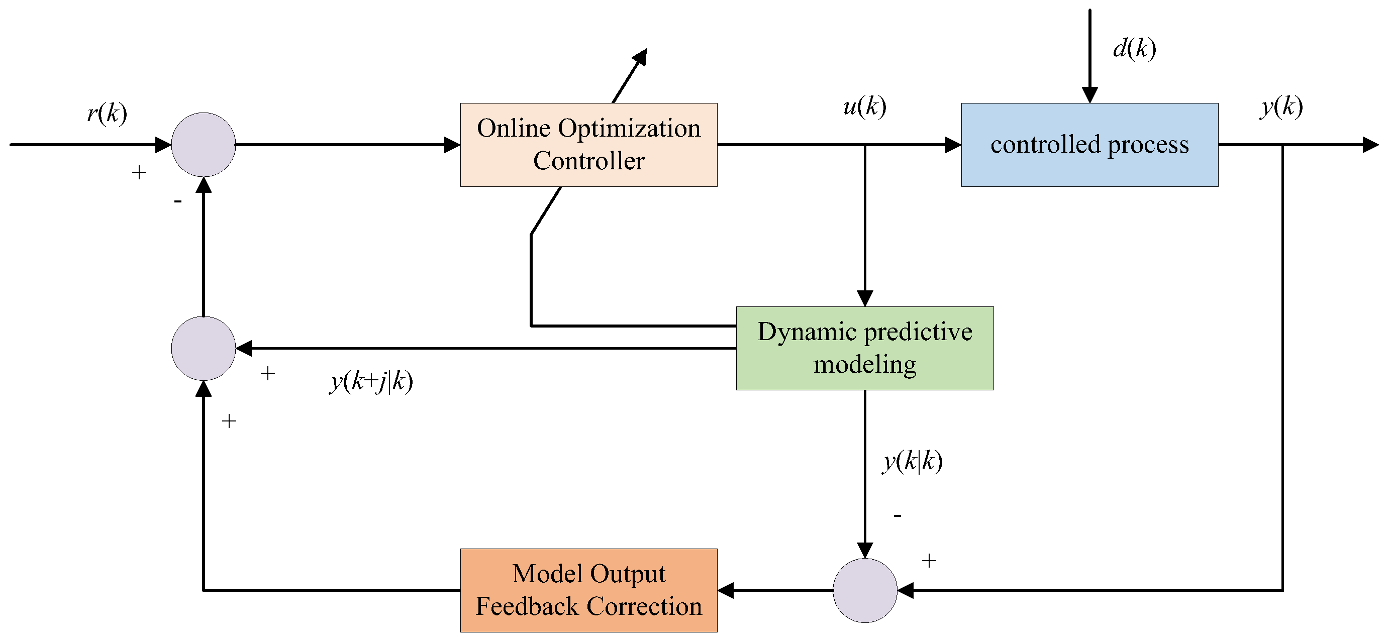
The MPC methodology constructs a state-space model or discrete transfer function to predict the dynamic response trajectory of a controlled object within a finite horizon. A convex optimization problem is solved online to minimize the objective function, generating an optimal control sequence that satisfies input/output constraints (control flowchart shown in Figure 2). A typical MPC cycle comprises three core stages: (1) model prediction, (2) online optimization, and (3) implementation of the first-step control action. By continuously updating the rolling horizon with real-time system state feedback, MPC effectively mitigates model mismatch and external disturbances, making it particularly advantageous in complex industrial processes, intelligent transportation systems, and robotic motion control.

Compared with conventional control strategies, MPC exhibits unique strengths in handling multivariate coupled systems, explicit constraint enforcement, and nonlinear dynamic optimization. Its multi-input multi-output (MIMO) architecture inherently coordinates synergistic actions among multiple actuators, while its ability to integrate process constraints directly into a quadratic programming framework guarantees optimal system operation within safety boundaries. For nonlinear time-varying systems, dynamic linearization can be achieved through sequential quadratic programming (SQP) or nonlinear MPC; however, the resultant exponential growth in computational complexity remains a bottleneck in practical engineering applications. Furthermore, the sensitivity of control performance to model accuracy necessitates online parameter estimation via system identification techniques, imposing stricter robustness requirements on control algorithms.

Current MPC technologies have demonstrated significant success in chemical process optimization, autonomous vehicle trajectory tracking, spacecraft attitude control, and building energy management. For instance, in continuous catalytic cracking units, MPC can coordinate temperature-pressure-flow multivariate systems to increase product yield by 3–5%. In autonomous driving, its rolling optimization capability enables effective obstacle avoidance and path planning under sudden disturbances. With advancements in edge computing hardware and distributed optimization algorithms, computational latency in MPC is progressively being alleviated. Future research will focus on data-driven model construction, distributed MPC architecture design, and the engineering application of quantum optimization algorithms. These breakthroughs are expected to drive deeper integration of MPC into complex systems such as smart manufacturing and smart cities.

As an advanced control strategy, MPC’s essence lies in its online solution of finite-horizon optimization problems to achieve effective control of dynamic systems. For discrete-time domains, the mathematical equation of MPC is expressed in Equation (19).

$$\left(\begin{array}{c}\begin{array}{c}\min \\ \mathrm{u}\end{array}J={\displaystyle \sum _{k=0}^{N_p-1}\Vert \mathrm{y}(}t+k\mid t)-\mathrm{r}(t+k){\Vert }_Q^2+{\displaystyle \sum _{k=0}^{N_c-1}\Vert \Delta \mathrm{u}(t+k){\Vert }_R^2}\\ \mathrm{s}.\mathrm{t}. \mathrm{x}(t+k+1)=f(\mathrm{x}(t+k),\mathrm{u}(t+k))\\ {\mathrm{u}}_{\min }\le \mathrm{u}\le {\mathrm{u}}_{\max }, \Delta {\mathrm{u}}_{\min }\le \Delta \mathrm{u}\le \Delta {\mathrm{u}}_{\max }\end{array} \right)$$

(19)

where, y denotes the system output variables, typically including hydropower generation, PV output, and bus voltage; r represents the reference trajectory, generally corresponding to the dispatch schedule in hydro-PV complementary systems; u signifies the control variables, often comprising turbine guide vane openings and PV inverter commands issued by the dispatch centre in such systems. N_p denotes the prediction horizon (in steps), typically set to 24 steps (equivalent to 24 h), while N_c is the control horizon (in steps), usually defined as N_c = N_p/2. The objective function J comprises two components. The term ${\displaystyle \sum _{k=0}^{N_p-1}‖y\left(t+k\left|t\right.\right)}-{r\left(t+k\right)‖}_Q^2$ minimizes the tracking error between the system output y and reference trajectory r, with the weighting matrix Q regulating the priority of different output variables; the term ${\displaystyle \sum _{k=0}^{N_c-1}‖\Delta u}{\left(t+k\right)‖}_R^2$ penalizes the magnitude of control increments Δu to ensure input smoothness and avoid abrupt actuator actions, where the weighting matrix R balances control energy consumption and tracking performance.

First, this composite objective function design embodies the trade-off between dynamic performance and robustness inherent in MPC. Second, constraints encapsulate both system dynamics and physical limitations. The state equation x(t + k + 1) = f(x(t + k), u(t + k) governs system evolution, whose form depends on model complexity (linear or nonlinear). Input constraints u_min ≤ u ≤ u_max directly reflect actuator physical limits (e.g., valve openings or motor torque boundaries), while increment constraints Δu_min ≤ Δu ≤ Δu_max restrict control input rates to prevent instability or mechanical wear caused by abrupt changes. The explicit handling of these constraints distinguishes MPC from conventional control methods. In practical applications, solving this optimization problem faces several challenges, listed as follows:

Prediction Horizon Selection: The prediction horizon N_t must balance computational efficiency with control performance. While extended horizons enhance accuracy (typically N_c = N_p/2), they escalate problem dimensionality, compromising real-time capability.

Nonlinear System Optimization: Non-convexity in nonlinear systems often necessitates sequential quadratic programming (SQP) or real-time iteration algorithms.

Weight Matrix Tuning: The calibration of Q and R requires iterative simulation or experimentation to ensure closed-loop stability and response speed.

Constraint Conflict Resolution: Infeasible scenarios due to conflicting constraints demand slack variables or priority-based constraint relaxation to enhance algorithmic robustness. Furthermore, MPC’s rolling optimization mechanism mandates state estimation updates and optimization re-solving at each sampling interval, imposing stringent requirements on computational hardware and real-time algorithms. To address this, explicit MPC or simplified linear time-invariant (LTI) models are often adopted in engineering practice to reduce complexity. Simultaneously, robust MPC or adaptive MPC frameworks can be integrated with online model updates or disturbance observers to mitigate model mismatch and external perturbations.

In summary, MPC achieves effective control of complex dynamic systems through multi-objective optimization and constraint handling. Its theoretical flexibility and engineering adaptability have enabled widespread applications in process control, robotic motion planning, and autonomous driving. Future research should focus on high-efficiency solvers, data-driven model identification, and integration with learning-based MPC to address higher-dimensional and highly uncertain control scenarios.

4.2. Rolling Optimization Mechanism for Collaborative System Modeling

Considering the rolling optimization requirements of hydro-photovoltaic collaborative systems, the hydro-power output P_h(t) model is expressed in Equation (20).

$$P_h(t)=\eta \cdot \rho \cdot g\cdot Q(t)\cdot H(t)$$

(20)

where, $P_h(t)$ represents the hydro-power output (kW or MW) at time t, with typical reference values ranging from 0.2 to 50 MW. This parameter can be obtained through real-time monitoring via the SCADA system. η denotes the comprehensive efficiency of the hydro turbine generator unit, typically ranging from 0.2 to 50 MW, which can be acquired from the technical specifications of the generator unit. ρ indicates water density (kg/m³) with conventional reference values between 0.2 and 50 MW. g represents the gravitational acceleration constant (9.81 m/s²). Q(t), the real-time discharge flow (m³/s), is jointly regulated by guide vane opening α(t) ∈ [0.2, 0.9] and reservoir capacity constraints V_min ≤ V(t) ≤ V_max. H(t) represents the net hydraulic head (dynamic water head) at time t, defined as the elevation difference between upstream and downstream water levels (m). Typical values range from 15 m to 300 m, measurable through water level sensor calculations.

For the rolling optimization requirements of hydro-photovoltaic collaborative systems, the photovoltaic output $P_{\mathrm{PV}}(t)$ model is expressed in Equation (21).

$$P_{\mathrm{PV}}(t)=G(t)\cdot A\cdot {\eta }_{\mathrm{PV}}\cdot {\eta }_{\mathrm{inv}}\cdot \left[1-0.0045\left(T_c(t)-25\right)\right]$$

(21)

where, $P_{\mathrm{PV}}(t)$ denotes the output power (kW) of the photovoltaic array at time t, typically ranging from 0 to rated capacity. This parameter can be measured through inverter output monitoring. $G(t)$ represents the tilted irradiance (W/m²) at time t, with conventional values between 0~1300 W/m², obtainable through pyranometer measurements or PV GIS database. A indicates the total area of the photovoltaic array (m²), derived from engineering design parameters. ${\eta }_{\mathrm{PV}}$ signifies the photovoltaic conversion efficiency, typically ranging from 0.15~0.22, which can be obtained from technical specifications of photovoltaic modules. $T_c\left(t\right)$ refers to the solar panel temperature (°C) at time t, generally varying between −20~70 °C, measurable through temperature sensors or predictable via weather forecasting models.

4.3. Multi-Objective Optimization Framework for Hydro-Photovoltaic Complementary Systems

The multi-objective optimization framework for hydro-photovoltaic complementary systems is designed to harmonize the integrated performance of the system across four dimensions: economic efficiency, environmental sustainability, operational stability, and equipment degradation. The mathematical expression of this multi-objective vector optimization problem is represented by Equations (22) and (23).

$$\begin{array}{l}{\min }_{\mathrm{u}}\mathrm{J}={\left[{\mathrm{J}}_1{,\mathrm{J}}_2{,,,\mathrm{J}}_{\mathrm{k}}\right]}^{\mathrm{T}}\\ \mathrm{s}.\mathrm{t}. \mathrm{g}\left(\mathrm{u}\right)\le 0, \mathrm{h}\left(\mathrm{u}\right)=0\end{array}$$

(22)

$$J=\left[\begin{array}{c}{J}_1\\ J_2\\ J_3\\ J_4\end{array}\right]=\left[\begin{array}{c}{\displaystyle \sum _{t=1}^{\tau }\left(C_{\mathrm{hyd}}+C_{\mathrm{pv}}+C_{\mathrm{grid}}+C_{\mathrm{battery}}\right)}\\ {\displaystyle \sum _{t=1}^{\tau }\left({\alpha }_{\mathrm{hyd}}{P}_{\mathrm{hyd},t}+{\alpha }_{\mathrm{grid} }{P}_{\mathrm{grid} ,t}\right)}\\ {\displaystyle \sum _{t=2}^{\tau }{\left(\Delta P_{t\mathrm{otal},t}\right)}^2}\\ {\displaystyle \sum _{t=1}^{\tau }\left({\eta }_{\mathrm{ch}}\left|P_{\mathrm{ch},t}\right|+{\eta }_{\mathrm{dis}}\left|P_{\mathrm{dis},t}\right|\right)}\end{array}\right].$$

(23)

where T is defined as the transition matrix; τ denotes the optimization variable; J₁ represents the total operational cost, encompassing joint expenses of hydropower, photovoltaics, grid interactions, and battery storage (where $C_{\mathrm{hyd}},C_{\mathrm{pv}},C_{\mathrm{grid}},C_{\mathrm{battery}}$ are denoted as the costs of hydropower, photovoltaics, grid transactions, and battery systems, respectively); J₂ quantifies the total carbon emissions of the system, considering only contributions from hydro-power and grid sources (with photovoltaic emissions assumed negligible, ${\alpha }_{\mathrm{hyd}}$ is defined as the hydropower emission coefficient, $P_{\mathrm{hyd},t}$ indicates hydropower-related emissions, ${\alpha }_{\mathrm{grid} }$ represents the grid emission coefficient, and $P_{\mathrm{grid} ,t}$ corresponds to grid-related emissions), whose Equation (21) is expressed through weighted coefficients; J₃ is modeled as a power fluctuation penalty term, calculated based on the difference in total power between consecutive time intervals (where $\Delta P_{t\mathrm{otal},t}$(t) denotes the power fluctuation deviation at time t); J₄ characterizes battery degradation, expressed as the accumulated product of absolute charging/discharging power and aging coefficients (where ${\eta }_{\mathrm{ch}},\left|P_{\mathrm{ch},t}\right|$ represent the aging coefficient and absolute charging power, respectively, while ${\eta }_{\mathrm{dis}},\left|P_{\mathrm{dis},t}\right|$ correspond to the aging coefficient and absolute discharging power), reflecting the negative correlation between battery lifespan and charge/discharge intensity.

The feasible solution region of the system is jointly determined by trade-offs among multiple objectives and constraint conditions in practical optimization. Economic efficiency (J₁) and environmental sustainability (J₂) are often contradictory; for instance, reducing carbon emissions may require increased reliance on clean energy, thereby elevating operational costs. Operational stability (J₃) and equipment degradation (J₄) are mutually constrained, as frequent power adjustments to suppress fluctuations may accelerate battery aging. Inequality constraints g(u) ≤ 0 and equality constraints h(u) = 0 are required to ensure power balance, equipment capacity limits (e.g., maximum hydro-power/photovoltaic outputs), and operational boundaries (e.g., battery charge/discharge rate thresholds). The multi-objective optimization problem is addressed using Pareto optimal solution generation methods (e.g., NSGA-II) or scalarization via weighted coefficients. Weight selection must align with system priorities and scenario-specific requirements. While the refined modeling of power fluctuations and battery degradation enhances long-term system reliability and cost-effectiveness, the inherent non-linearity increases computational complexity. To mitigate this, intelligent optimization algorithms (e.g., meta-heuristics) or convex relaxation strategies are recommended to improve solving efficiency.

The decision variable u, which is defined as the core parameter governing the energy dispatch strategy across time intervals is expressed in Equation (24).

$$u=\left[\begin{array}{c}{P}_{\mathrm{hyd},1},\dots ,P_{\mathrm{hyd},T}\\ P_{\mathrm{pv},1},\dots ,P_{\mathrm{pv},T}\\ P_{\mathrm{grid},1},\dots ,P_{\mathrm{grid},T}\\ P_{\mathrm{ch},1},\dots ,P_{\mathrm{ch},T}\\ P_{\mathrm{dis},1},\dots ,P_{\mathrm{dis},T}\end{array}\right].$$

(24)

The decision variable u is structured as a column vector comprising five sub-vectors, corresponding to the hydropower output P_hyd,t, photovoltaic output P_pv,t, grid interaction power P_grid,t, battery charging power P_ch,t, and discharging power P_dis,t across time intervals t = 1,2, …, T. This architecture is designed to address the multi-energy coordination requirements of the system, where hydropower and photovoltaics serve as renewable energy sources, grid interaction power characterizes external energy exchange, and battery charge/discharge power is utilized to mitigate fluctuations and enable energy time-shifting. Each sub-variable is required to be continuously optimized temporally to achieve dynamic supply-demand balance and accommodate multi-objective optimization demands.

The design of decision variables must rigorously integrate the inter-dependencies between physical constraints and optimization objectives. Regarding technical limitations, hydro-power and photovoltaic power are constrained by natural resource availability (e.g., water flow, solar irradiance) and equipment capacity limits. Grid interaction power is governed by grid connection protocols, including power limits and electricity pricing mechanisms. Battery charge/discharge power is subject to mutual exclusivity constraints (P_ch,t, P_dis,t = 0) to prevent efficiency losses from simultaneous charging and discharging. For dynamic inter-variable coupling, increasing photovoltaic power may reduce J₂ (carbon emissions) but could intensify power fluctuations, thereby elevating battery regulation frequency and exacerbating J₃ (stability penalty) and J₄ (degradation cost). Temporal horizon selection requires that the period T is optimized to balance prediction accuracy and computational complexity. Short-term optimization might overlook long-term economic efficiency, whereas long-term optimization necessitates addressing uncertainties in renewable energy forecasts.

These characteristics collectively render the feasible domain high-dimensional and non-convex. To address this, intelligent optimization algorithms (e.g., evolutionary strategies) or hierarchical solving frameworks are employed for efficient solution identification. Equation (25) formulates the multi-objective optimization model of the hydro-photovoltaic system, incorporating rigorous mathematical constraints.

$$\left\{\begin{array}{ll}{P}_{\mathrm{hyd},min}-P_{\mathrm{hyd},t}\le 0\hfill & \hfill \\ P_{\mathrm{hyd},t}-P_{\mathrm{hyd},max}\le 0\hfill & \hfill \\ {\displaystyle {\sum }_{t=1}^T{P}_{\mathrm{hyd},t}}\Delta t-W_{\mathrm{total} }\le 0\hfill & \hfill \\ SO{C}_{min}-SO{C}_t\le 0\hfill & \hfill \\ SO{C}_t-SO{C}_{max}\le 0\hfill & \hfill \\ -P_{\mathrm{grid},t}-P_{\mathrm{sell},max}\le 0\hfill & \hfill \\ P_{\mathrm{grid},t}-P_{\mathrm{buy},max}\le 0\hfill & \hfill \end{array}\right.$$

(25)

The multi-objective optimization model for hydro-PV complementary systems achieves economic and environmental operational objectives through rigorously constructed mathematical constraints. Within the inequality constraint component g(u) ≤ 0, the system’s physical boundaries and operational rules are enforced across multiple dimensions. The real-time hydro-power output $P_{\mathrm{hyd},t}$ is constrained by the upper and lower bounds to ensure hydro units operate within rated capacity ranges, thereby preventing equipment overload or inefficient operating conditions. The total reservoir water volume $W_{\mathrm{total} }$ imposes hard constraints reflecting water resource limitations, requiring available water to be rationally allocated throughout the scheduling cycle. The energy storage system’s state of charge ($SO{C}_t$) must be maintained within a secure operational interval to prevent battery over-charging or over-discharging, consequently extending service life. The upper and lower bounds of selling power $P_{\mathrm{sell}, \max }$ and purchasing power $P_{\mathrm{buy} ,\max }$ are governed by generation limitations under extreme weather conditions and the economic boundaries of grid-interactive power $P_{\mathrm{grid},t}$, respectively, ensuring system stability during external environmental fluctuations. These inequality constraints collectively define the feasible operational region of the system, guaranteeing physical feasibility for multi-objective optimization. The mathematical formulation of the power balance equation is expressed in Equation (26).

$$\left\{\begin{array}{ll}{P}_{\mathrm{hyd},t}+P_{\mathrm{pv},t}+P_{\mathrm{grid},t}+P_{\mathrm{dis},t}-P_{\mathrm{ch},t}-P_{\mathrm{load},t}=0\hfill & \hfill \\ SO{C}_t-SO{C}_{t-1}-\left({\displaystyle \frac{{\eta }_{\mathrm{ch}}{P}_{\mathrm{ch},t}}{E_{\mathrm{bot} }}}-{\displaystyle \frac{P_{\mathrm{dis},\mathrm{t} }}{{\eta }_{\mathrm{dis} }{E}_{\mathrm{bot} }}}\right)\Delta t=0\hfill & \hfill \end{array}\right.$$

(26)

The equality constraint h(u) = 0 inherently reinforces the internal correlations of the system from the perspectives of energy conservation and dynamic equilibrium. The power balance equation requires that the combined output from multiple energy sources, including hydro, photovoltaic, storage, and the grid, matches the load demand in real time, thereby avoiding power deficits or surpluses. The dynamic state-of-charge (SOC) equation for the battery quantifies the variation pattern of the energy storage status, providing a dynamic model foundation for cross-period energy scheduling. C_hyd denotes the hydro generation cost function (¥/MWh), which is determined by the quadratic function $a{P}_{h\mathrm{yd},t}^2+b{P}_{\mathrm{hyd},t}+c$, α_grid represents the carbon emission intensity of grid power (kgCO₂/MWh); η_ch/dis indicates the battery charging/discharging efficiency; E_bat is the rated battery capacity (MWh); W_total signifies the total available reservoir water volume (MWh); and Δt is the time interval (h).

The quadratic growth characteristic of cost with respect to power output necessitates that generation revenue and marginal cost must be balanced during optimization. Conversely, the incorporation of grid electricity carbon emission intensity C_hyd highlights the model’s consideration for low-carbon objectives. The time interval Δt, serving as a discretization parameter, transforms the continuous dynamic problem into a sequential optimization problem. Collectively, these equality constraints and variable definitions constitute the mathematical core of the system’s multi-objective optimization, establishing the theoretical framework for solving the economic-environmental dual-objective Pareto front.

The multi-objective optimization model for hydro-PV complementary systems requires the reconciliation of conflicting objectives, including economy, environmental sustainability, and operational stability, through mathematical methods. To address dimensional disparities among objective functions (e.g., cost, carbon emissions), normalization processing is applied to J₁, J₂, J₃, and J₄. A linear transformation maps each objective value to the [0, 1] interval, eliminating dimensional influences and providing a comparable basis for multi-objective trade-offs. The expression for the normalization process is expressed in Equation (27).

$${\tilde{J}}_i={\displaystyle \frac{J_i-J_{i,min}}{J_{i,max}-J_{i,min}}}$$

(27)

The weighted aggregation method, by incorporating preference weights w_i, converts the multi-objective problem into a single-objective optimization problem, i.e., it is expressed in Equation (28).

$$\min {\displaystyle \sum _{i=1}^4{w}_i}{\tilde{J}}_i \left( {\displaystyle \sum w_i}=1\right)$$

(28)

Should the actual objective be the minimization of the sum of squared weights, this may implicitly impose a constraint on the uniformity of weight distribution, thereby preventing any single objective from exerting excessive dominance. Moreover, the setting of weights must be integrated with the prioritization of the hydro cost function C_hyd and the carbon emission intensity C_gdd. For instance, under low-carbon policy directives, a higher weight may be assigned to the carbon emission reduction target. These methodologies are required to be solved in coordination with the previously established constraints (e.g., the power balance equation and the SOC dynamic equation) to ensure that the optimization outcomes simultaneously satisfy physical feasibility and multi-objective equilibrium.

A comparison of the solution algorithms (e.g., NSGA-II, MOEA/D, weighted particle swarm optimization, and robust optimization) is presented in

Table 8. Comparison of Solution Algorithms.

Algorithm	Applicable Scenario	Hydro-PV System Applicability
NSGA-II	High-dimensional Pareto front solution	★★★★★
MOEA/D	Strong inter-objective coupling	★★★★☆
Weighted Particle Swarm	Real-time control requirements	★★★☆☆
Robust Optimization	Considering prediction uncertainty	★★★★☆

.

In the Pareto front solution, algorithm selection directly influences optimization efficiency and the quality of the solution set. NSGA-II efficiently handles high-dimensional objective spaces through non-dominated sorting and crowding distance mechanisms, rendering it suitable for the multi-objective characteristics of hydro-PV systems with a five-star applicability rating in Table 8 [33]. Note: Performance rating symbols: ★ (filled star) denotes superior effectiveness (★ quantity ∝ performance level); conversely, ☆ (unfilled star) indicates inferior effectiveness (☆ quantity ∝ performance degradation). Its advantage lies in its strong global search capability, enabling the generation of uniformly distributed Pareto solution sets that support decision-makers in selecting optimal trade-off solutions based on real-time requirements. In contrast, MOEA/D (multi-Objective evolutionary algorithm based on decomposition) transforms the multi-objective optimization problem (MOP) into a set of single-objective subproblems through decomposition strategies, approximating the Pareto front via collaboration among subproblems. MOEA/D handles strongly coupled problems through objective function decomposition, exhibiting slightly lower applicability (four stars), but potentially outperforming others when significant interactions exist between objectives. Weighted particle swarm optimization (three stars) is suitable for real-time control scenarios but struggles to guarantee solution set diversity and convergence. Robust optimization (four stars) accommodates prediction uncertainties (e.g., PV output fluctuations) at the expense of computational efficiency. Collectively, NSGA-II and MOEA/D are more appropriate for long-term scheduling optimization, while scenarios with high real-time requirements may incorporate particle swarm algorithms for local adjustments. Algorithm selection must further consider model complexity factors, such as the discretization step size Δt in the SOC dynamic equation and computational resource constraints, to achieve a balance between optimization accuracy and efficiency. These methodologies provide critical technical support for translating theoretical models of hydro-PV complementary systems into practical applications.

4.4. Feedback Correction Strategy for Hydro-PV Complementary Systems

The unique design of hydro-PV complementary systems significantly enhances uncertainty resilience through the integration of multi-timescale feedback mechanisms, anti-disturbance strategies, and advanced data assimilation techniques. As detailed in

Table 9. Multi-timescale feedback design.

Timescale	Feedback Variable	Corrective Action
15-min	Actual vs. forecasted PV output	Adjustment of inverter clipping coefficient
Hourly	Hydro-regulation deviation	Correction of the hydro unit efficiency model parameters
Daily	Accumulated reservoir water level error	Update of inflow prediction model parameters

, the multi-timescale feedback design implements hierarchical correction for disturbances across different temporal dimensions. At the 15-min level, real-time PV output is compared with the forecasted values. Fluctuations caused by cloud occlusion are mitigated through dynamic adjustment of the inverter clipping coefficient M_max to limit power overshoot and ensure equipment safety.

At the hourly level, dydro-regulation deviations (e.g., unit efficiency model errors or water flow variations) are addressed by refining hydro unit efficiency models via parameter identification algorithms, thereby improving output accuracy.

At the daily level, accumulated reservoir water level errors (e.g., from precipitation forecast deviations or evaporation losses) are corrected through updates to input parameters of inflow prediction models, optimizing long-term water dispatch schedules.

This hierarchical mechanism achieves full-cycle coverage from second-scale disturbances to long-term trends, effectively balancing system responsiveness with global optimization requirements.

Regarding anti-disturbance mechanisms, a closed-loop control strategy is employed for abrupt scenarios such as irradiation plunges; $u_h$ is expressed in Equation (29).

$$\Delta u_h=K_p\cdot \left(P_{\mathrm{PV}}^{\mathrm{pred} }-P_{\mathrm{PV}}^{\mathrm{meas} }\right)$$

(29)

where $P_{\mathrm{PV}}^{\mathrm{pred} }$ represents the forecasted PV generation power, while $P_{\mathrm{PV}}^{\mathrm{meas} }$ denotes the measured PV generation power. The hydro regulation gain K_p (typical value: 0.5 MW/%) enables hydropower output to be dynamically adjusted, facilitating rapid compensation for PV power deficits and maintaining power balance.

Data assimilation techniques are implemented through the ensemble Kalman filter (EnKF), which integrates real-time observational data (e.g., reservoir inflow rates, PV output) with model predictions. This process iteratively updates the state estimation vector x_i, significantly reducing prediction uncertainty. The data assimilation is expressed in Equation (30).

$$x_t^a=x_t^f+K_t\left(y_t-H{x}_t^f\right)$$

(30)

where $x_t^a$ denotes the optimal state estimate after data assimilation. This analysis field integrates model predictions with actual observational data, representing the most accurate estimation of the system’s current state. $x_t^f$ signifies the prior forecast result generated by the model based on historical data or the previous state, constituting the state estimate before real-time observations are incorporated. K_t represents the Kalman gain matrix that quantifies the weighting ratio between observational data and model predictions. Its magnitude is governed by both models’ forecast error covariance and observation error covariance, determining the degree of observational corrections to the final analysis. y_t corresponds to actual measured values (e.g., reservoir inflow rates, PV output)—physical quantities acquired in real time for model prediction correction. H denotes the observation operator, which may be a linear or nonlinear function mapping state variables to the observation space, serving to extract observable quantities from the model-predicted state. Typical control effects are presented in

Table 10. Typical control effects.

Scenario	Baseline Fluctuation Rate	Post-MPC Fluctuation Rate	Improvement Magnitude
PV cloud occlusion	32%	18%	43.8%
Load surge	28%	15%	46.4%
Unit failure	41%	23%	43.9%

.

Analysis of Table 10 reveals that MPC implementation reduces system fluctuation rates by 43.8%, 46.4%, and 43.9% under PV cloud occlusion, load surge, and unit failure scenarios, respectively, thereby verifying the effectiveness of the aforementioned strategies. The optimized design of the Kalman gain K_i enables adaptive adjustment of weighting between observational data and model predictions, particularly excelling in scenarios involving significant nonlinearities such as reservoir inflow prediction. These techniques not only enhance system robustness but also provide real-time dynamic support for multi-objective optimization models (e.g., Pareto solution sets generated by NSGA-II), ensuring operational feasibility of theoretical optimization outcomes in practical implementations.

5. Case Study Verification and Analysis

5.1. Case Data Preprocessing

Distributed PV generation data, comprising parameters such as irradiance ($G_t,{ \mathrm{W}/\mathrm{m}}^2$), module temperature ($T_t,℃$), and output power ($P_{\mathrm{PV},t}$, $\mathrm{kW}$), were first subjected to outlier cleaning, resulting in P_PV,clean. Subsequently, the theoretical predicted value of PV output power at time t (${\widehat{P}}_{\mathrm{PV},t}$, kW) was calculated. The following data were obtained: rated power $P_{rated}$ = 100 kW, historical residual standard deviation σ = 8.2 kW, measured PV output power at a specific time $P_{\mathrm{PV},t}$ = 62 kW, and the theoretical predicted value at time t ${\widehat{P}}_{\mathrm{PV},t}$ = 85 kW, calculated using Equation (4). The outlier cleaning decision process for distributed PV generation data, as defined by Equation (4), is expressed in Equation (31). Consequently, the cleaning result is given by Equation (32).

$$|62-85|=23 \mathrm{kW}>3\times 8.2=24.6\mathrm{kW}$$

(31)

$$P_{\mathrm{PV}, \mathrm{clean} }=85\mathrm{kw}$$

(32)

For a systematic evaluation of data cleaning methods,

Table 11. Comparison of Different Data Cleaning Methods.

Method	Formula Characteristics	Advantages	Disadvantages
3σ Criterion	${\widehat{P}}_{\mathrm{PV},t}=G_t\cdot \eta \cdot A\cdot \left[1-0.005\left(T_t-25\right)\right]$	Clear statistical significance	Relies on the normal distribution assumption
Interquartile Range (IQR) Method	Threshold: 1.5 × IQR	Strong outlier resistance	Requires quartile computation
Moving Average	Replaces with neighborhood mean	Simple and fast	Obscures true fluctuation characteristics
Machine Learning	Predicts valid range via LSTM	Adapts to complex patterns	Requires extensive training data

compares four mainstream approaches. The 3σ criterion defines the outlier range based on statistical normal distribution assumptions, offering clear statistical significance and computational simplicity. However, its reliance on normality assumptions may cause misjudgement in asymmetric distributions [21]. The interquartile range (IQR) method identifies outliers using a non-parametric approach with a 1.5 × IQR threshold, demonstrating strong interference resistance, particularly suitable for datasets containing extreme values. Nevertheless, it requires additional quartile calculations, resulting in slightly higher computational complexity [22]. The moving average method replaces anomalies with adjacent time-period means, providing rapid processing advantages but potentially smoothing genuine fluctuation features, thereby distorting time-series dynamics [23]. Machine learning methods, such as LSTM models, predict valid power ranges through training, capturing complex nonlinear relationships with strong adaptability. However, they demand substantial annotated data and exhibit low model interpretability [24].

Comprehensive analysis indicates that the 3σ criterion is preferred for PV data cleaning due to its clear theoretical basis and ease of implementation. Nevertheless, single methods possess limitations. For instance, during nighttime zero-output periods, theoretical values may deviate from actual conditions, necessitating supplementary artificial rules (e.g., enforcing zero-power constraints at night). Furthermore, hybrid approaches can enhance robustness. IQR-based preliminary outlier screening may be followed by moving average correction for short-term fluctuations, with machine learning models subsequently optimizing long-term trend predictions. In summary, PV data cleaning constitutes a fundamental process for ensuring renewable energy system reliability. This multi-method comparison demonstrates the practical value of combining the 3σ criterion with artificial rule verification, while highlighting machine learning’s potential in future big-data environments. Future research could explore hybrid cleaning frameworks integrating statistical methods and deep learning models to achieve higher-precision anomaly detection and data reconstruction, thereby providing more robust data support for hydro-PV hybrid systems optimization.

Similarly, comparisons between data cleaning methods and other standardization approaches are presented in

Table 12. Comparison with Other Standardization Methods.

Method	Formula	Applicable Scenario	Suitability for Hydro-PV Research
Min–Max	$Q_{\mathrm{norm} ,t}={\displaystyle \frac{Q_t-Q_{\min }}{Q_{\max }-Q_{\min }}}$	Clear data boundaries	★★★★★
Z-score	${\displaystyle \frac{Q_t-\mu }{\sigma }}$	Gaussian-distributed data	★★☆☆☆
Decimal Scaling	${\displaystyle \frac{Q_t}{{10}^k}}$	Extremely large numerical ranges	★☆☆☆☆
Robust Scaling	${\displaystyle \frac{Q_t-Q_{\mathrm{median} }}{Q_{75}-Q_{25}}}$	Presence of outliers	★★★★☆

.

As analyzed in Table 12, regarding suitability for hydro-PV complementary research, the min–max method is rated five stars owing to its advantage of clear data boundaries. Note: Performance rating symbols: ★ (filled star) denotes superior effectiveness (★ quantity ∝ performance level); conversely, ☆ (unfilled star) indicates inferior effectiveness (☆ quantity ∝ performance degradation). The robust scaling method is rated four stars due to its applicability in the presence of outliers. The Z-score and decimal scaling methods, suitable for Gaussian-distributed data and extremely large numerical ranges, respectively, are rated one star because they are considered unsuitable for standardizing hydro-PV complementary data. The min-max method is prioritized as it better complies with the input requirements of copula functions (i.e., the [0, 1] interval). The robust scaling method is selected as an alternative when extreme outliers are present in the data.

5.2. Multi-Scale Characteristic Analysis of Hydro-PV Complementary System

(1)

Validation and Analysis of Daily Complementarity Index

To validate the theory of the daily complementarity index (C_daily), which quantifies the temporal complementarity between photovoltaic and hydropower at the daily scale, photovoltaic power is regarded as the dominant source, while hydropower serves as the regulating source. Photovoltaic output is adopted as the baseline due to its stronger volatility. The measured data for deriving C_daily are presented in

Table 13. Measured Data for Daily Complementarity Index Cdaily.

Time Point	$P_{\mathrm{hydro}}$	$P_{\mathrm{PV}}$	$\parallel P_{\mathrm{hydro}}-P_{\mathrm{PV}}\parallel$
08:00	0.450	0.320	0.130
12:00	0.280	0.910	−0.630
18:00	0.820	0.050	0.770
∑	-	9.86	7.24

.

Based on Table 13, the daily complementarity index $C_{daily}$ is expressed in Equation (33).

$$C_{\mathrm{daily} }=1-{\displaystyle \frac{7.24}{2\times 9.86}}=0.63$$

(33)

Analysis of data from a hydropower station in Yunnan using this theoretical approach indicates that $C_{daily}\approx 0.62$ during the dry season and $C_{daily}\approx 0.81$ during the wet season. The application criteria for the daily complementarity index $C_{daily}$ are summarized as follows:

Poor complementarity ($C_{daily}<0.3$): Energy storage integration is required.

Moderate complementarity ($0.3\le C_{daily}<0.6$): Hybrid operation is feasible without immediate storage expansion.

Strong complementarity ($C_{daily}\ge 0.6C$): The station demonstrates robust hydro-PV complementary capability.

Comparisons between C_daily and other complementarity metrics are provided in

Table 14. Comparison of Daily Complementarity Index C_daily with Other Metrics.

Metric	Formula Characteristics	Advantage	Limitation
Cdaily	$C_{\mathrm{daily}}=1-{\displaystyle \frac{{\displaystyle \sum _{t=1}^{24}\left|P_{\mathrm{hydro},t}-P_{\mathrm{PV},t}\right|}}{2{\displaystyle \sum _{t=1}^{24}{P}_{\mathrm{PV},t}}}}$	Intuitively reflects daily-scale matching.	Neglects short-term fluctuations
Correlation Coefficient ρ	${\displaystyle \frac{\mathrm{Cov}\left(P_{\mathrm{hydro}},P_{\mathrm{PV}}\right)}{{\sigma }_{\mathrm{hydro}}{\sigma }_{\mathrm{PV}}}}$	Clear statistical significance	Captures only linear relationships.
Complementary Energy Ratio	${\displaystyle \frac{{\displaystyle \sum \min }\left(P_{\mathrm{hydro}},P_{\mathrm{PV}}\right)}{{\displaystyle \sum P_{\mathrm{PV}}}}}$	Clear physical meaning	Fails to distinguish peak/valley scenarios

.

Analysis of Table 14 indicates that the C_daily method is prioritized for resource matching assessment in planning stages. For real-time control, it is recommended to combine C_daily with the hourly fluctuation rate η_1h for comprehensive analysis.

(2)

Validation Analysis of Seasonal Wet–Dry Complementarity

As derived from Equation (31), the seasonal wet–dry complementarity difference coefficient k quantifies the impact of hydrological seasonality on power output. A positive k indicates higher output in wet seasons than dry seasons (typical runoff hydropower), while a negative value signifies anti-seasonal characteristics (e.g., snowmelt-fed hydropower). Normalization by P_annual enables cross-station comparisons (e.g., Station A: k = 0.3 vs. Station B: k = 0.6). Extreme cases include k→1: near-zero dry-season output (e.g., unregulated reservoirs); k→−1: anomalous seasonal behavior (data rationality should be verified).

The case study data were analyzed as follows: wet-season average output: P_wet = 650 kW; dry-season average output: P_dry = 180 kW; annual average output: P_annual = 420 kW. The seasonal wet-dry complementarity difference coefficient is expressed in Equation (34).

$$\kappa ={\displaystyle \frac{650-180}{420}}=1.12$$

(34)

Analysis of the hydropower station demonstrates that a seasonal wet–dry complementarity difference coefficient k > 1 indicates that the wet-season output significantly exceeds the annual average.

The evaluation criteria utilizing k are summarized as follows:

• 0 < k < 0.2: Weak seasonality (suitable for baseload operation);
• 0.2 < k < 0.5: Moderate seasonality;
• k > 0.5: Strong seasonality (requires complementary storage or generation sources).

5.3. Validation Analysis of Spatial Complementarity Characteristics

(1)

Cascade Comprehensive Regulation Benefit Index

To validate the cascade comprehensive regulation benefit index β for characterizing basin-scale distributed hydropower systems, basin data were substituted into Equation (16). A calculation example of β for a specific basin is presented in

Table 15. Calculation Example of Cascade Comprehensive Regulation Benefit Index β for a Specific Basin.

Power Station	Regulation Type	${\mathit{\alpha }}_{\mathit{i}}$	hi (m)	αihi
1#	Annual regulation	1.0	120	120
2#	Daily regulation	0.6	85	51
3#	No regulation	0	65	0

. The resulting β value is expressed in Equation (35).

$$\beta ={\displaystyle \frac{120+51+0}{120+85+65}}={\displaystyle \frac{171}{270}}=0.63$$

(35)

(2)

Analysis and Validation of PV Array Diversity Gain Index

To validate the diversity gain index D_PV for characterizing spatial distribution clusters of PV arrays, data from a specific PV array spatial distribution cluster were substituted into Equation (19). The example calculation of D_PV for the PV array spatial distribution cluster is presented in

Table 16. Measured Values for PV Diversity Gain Index D_PV.

Power Station	σi (kW)	Spatial Distribution
1#	120	Eastern
2#	85	Western
3#	60	Southern
Cluster total output standard deviation	σPV,total = 210 kW

. The resulting D_PV value is expressed in Equation (36).

$$D_{PV}=1-{\displaystyle \frac{210}{120+85+60}}=1-0.792=0.208$$

(36)

(3)

Hydro-PV Spatial Matching Index

The hydro-PV spatial matching index M was validated for evaluating spatial coordination by substituting interpolated hydrologic station data from a hydro-power plant and GIS-based irradiance data with terrain slope parameters from a PV plant into Equation (13). A calculation example is provided in

Table 17. Sample Data for Hydro-PV Spatial Matching Index M.

Grid ID	fhydro (kW/km2)	fPV (kW/km2)	Product fhydro fPV
1	120	80	9600
2	60	150	9000
3	0	200	0
∑	Phydro = 180	PPV = 430	18,600

, with the resulting M value given by Equation (37).

The engineering application framework based on M is summarized as follows:

M > 0.7: Priority development zones (e.g., Lancang River cascade + slope PV in Yunnan);

M < 0.3: Transmission infrastructure is required (e.g., geographically separated hydro-PV configuration in Tibet).

The hydro-PV spatial matching index M is expressed in Equation (37).

$$M={\displaystyle \frac{18,600\times 1{\mathrm{km}}^2}{\max (180,430)}}={\displaystyle \frac{18,600}{430}}\approx 0.43$$

(37)

The M-based hydro-PV coordinated planning methodology is structured around three core dimensions (Figure 3):

(1)

Planning Layout Optimization Strategy

During renewable project siting, a hierarchical decision-making mechanism is recommended, as follows:

Level I (M > 0.5): High complementarity regions are prioritized for distributed PV clusters with local consumption facilities, enhancing renewable penetration rates.

Level III (M < 0.2): Hydro-power scheduling radius should be re-evaluated. Cross-regional consumption capability is enhanced through coordinated cascade hydropower operation (±20 km dynamic adjustment range).

(2)

Hierarchical Decision Support System

A three-dimensional decision model incorporating spatial matching, temporal coupling, and capacity matching coefficients was developed, based on Table 6. This model enables spatial visualization via GIS platforms (Figure 3), identifying hydro-PV synergy potential at 500 m × 500 m grid resolution.

(3)

Dynamic Regulation Mechanism

An intelligent decision system (Figure 2) establishes a closed-loop “assessment-planning-validation” workflow. Real-time hydrological forecasts and PV output predictions are integrated, with the matching matrix updated at 6 h intervals to ensure spatiotemporal adaptability.

5.4. Probabilistic Theory Validation Based on Copula

The Gumbel–Clayton hybrid copula method is recommended for hydro-PV complementarity analysis, as it characterizes the asynchronous features of PV peak output (upper tail) and hydropower dry-season output (lower tail). Parameters from a hybrid power station case study in Yunnan are listed as follows:

(1)

Marginal distributions: PV output modelled with Beta distribution (α = 0.85, β = 0.62); hydropower described by Gamma distribution (k = 3.2, θ = 0.4).

(2)

Copula function: Time-varying Gumbel (θ ∈ [1.8, 3.1]) with fitting performance including clear-sky upper tail dependence λu = 0.71, rainy-day lower tail dependence λI = 0.43. The parameter estimation data for the probability density function $f\left(P_{PV};\alpha ,\beta \right)$ in a practical application scenario at a photovoltaic power station are presented in

Table 18. Engineering Application Data for PV Probability Density Function $f\left(P_{PV};\alpha ,\beta \right)$ Parameter Estimation.

Weather Type	α	β	Probability of PV Output in the Lower Tail (P < 0.1)	Probability of PV Output in the Upper Tail (P > 0.9)
Sunny	0.82	0.58	34%	41%
Cloudy	1.15	1.32	18%	12%
Rainy	2.10	0.95	6%	3%

.

5.5. Validation and Analysis of Multi-Scale Copula-MPC Predictive Control Method

The discretized state-space model of the hydro-photovoltaic complementary control system is constructed with generator rotor angle (δ), speed deviation (ω), mechanical torque (m_t), and guide vane opening (y) as state variables. Key parameters are listed in

Table 19. Key Parameters of Discretized State-Space Model.

Matrix Element	Physical Significance	Value	Unit/Derivation
A(1,2)	Rotor angle–speed coupling	314	=wB
A(2,2)	Speed self-attenuation coefficient	−0.222	−D/Ta
A(2,3)	Torque–speed transfer	0.111	1/Ta
A(3,3)	Torque self-attenuation	−2.0	−1/(eqhxTw)
A(3,4)	Guide vane–torque transfer	2.0	ey/(eqhxTw)
A(4,4)	Guide vane self-attenuation	−10.0	−1/Ty
B(3)	Control–torque transfer	−5.0	−emxey/(eqhxTy)
B(4)	Control–guide vane transfer	10.0	−1/Ty

.

As described in Table 19, the state matrix A embodies complex coupling between state variables. The value A(1,2) = 314 reflects the synchronous operation constraint of run-of-river small hydro generators. A(2,2) = −0.222 indicates inherent damping characteristics that enable self-stabilization without control input. Negative values A(3,3) = −2.0 and A(4,4) = −10.0 demonstrate turbine and governor stability. The input matrix B is designed considering control signal propagation paths. B(3) = −5.0 signifies negative feedback control on mechanical torque, consistent with hydraulic regulation mechanisms. B(4) = 10.0 reflects the high-gain characteristics of modern electro-hydraulic governors.

Comparative experiments were implemented using a fuzzy PID algorithm with parameters: fuzzification factors K_e = 0.9, K_{ec} = 0.1; defuzzification factors K_1 = 3, K_2 = 1.2, K_3 = 0.01; sampling period T = 0.01 s. The parameters in

Table 20. Initial Parameters of Fuzzy PID Algorithm.

Parameter	Value	Physical Significance	Design Consideration
KP	5.0	Proportional gain	Ensures rapid response
Ki	2.0	Integral gain	Eliminates steady-state error (Note 1)
Kd	0.1	Derivative gain	Enhances dynamic performance

balance rapidity and stability requirements.

The proportional gain K_P = 5.0 was set according to open-loop gain characteristics, where excessive values may induce overshoot while insufficient values cause sluggish response. Integral gain K_i = 2.0 effectively eliminates frequency deviation steady-state error but requires anti-windup measures. The relatively small derivative gain K_d = 0.1 improves dynamic response while avoiding high-frequency noise amplification.

The linear quadratic regulator (LQR) was designed by minimizing a quadratic cost function. Weighting matrices are configured in

Table 21. LQR Design Parameters.

Matrix	Value	Physical Significance	Design Consideration
$Q_{lqr}$	diag([10, 1, 1, 1])	State weighting	Prioritizes frequency stability
$R_{lqr}$	0.01	Control input weighting	Permits larger control effort

.

$Q_{lqr}$, the speed deviation weight (10), significantly exceeds other states (rotor angle: 1, torque: 1, guide vane: 1), emphasizing the importance of stable frequency. The small $R_{lqr}$ = 0.01 allows greater control action for enhanced dynamics.

Core parameters of the copula-MPC algorithm are detailed in

Table 22. Copula-MPC Design Parameters.

Parameter	Value/Dimension	Physical Significance	Design Consideration
N	10	Prediction horizon	Balances accuracy and computation
Ts	0.01 s	Sampling time	Meets real-time requirements
Qmpc	4 × 4	diag([200, 200, 200, 200])	Enhances reference tracking
Fmpc	4 × 4	diag([300, 300, 300, 300])	Ensures stability
Rmpc	1 × 1	0.01	Optimizes actuator effort

.

The prediction horizon N = 10 was selected through a trade-off between system dynamic response time and computational complexity. An excessively short prediction horizon prevents full utilization of model information, while an extended horizon increases computational burden. The sampling time Ts = 0.01 s ensures real-time control capability while satisfying Nyquist sampling theorem requirements. All diagonal elements of the state-weighting matrix Qmpc were set to 200, significantly larger than in the LQR algorithm, reflecting higher state-tracking precision requirements for copula-MPC. The terminal weighting matrix Fmpc = 300 further emphasizes the importance of terminal states at the prediction horizon end, enhancing closed-loop stability. Physical constraints for the copula-MPC algorithm are implemented as detailed in

Table 23. Copula-MPC Constraints.

Constraint Type	Lower Bound	Upper Bound	Physical Significance
Control input	−1.0 p.u.	+1.0 p.u.	Governor output limits
State variables	No constraints	No constraints	Optimization problem simplification
θ(t)	1.8	3.2	Time-varying Gumbel copula (Note 2)

; these reflect actual system limitations. Constraint settings reflecting physical limitations are given in Table 23.

The control input range [−1.0, +1.0] p.u. reflects practical governor saturation limits, enabling effective handling of actuator nonlinearities. The time-varying Gumbel copula (θ ∈ [1.8, 3.2]) demonstrates tail dependence indices ${\lambda }_U$ = 0.71 (clear sky) and ${\lambda }_L$ = 0.43 (rainy conditions).

(1)

Equilibrium Point Stabilization Verification

To validate the superiority of the proposed control algorithm, copula-MPC was compared with Fuzzy PID and LQR. Initial state values [δ, ω, m_t, y]^T = [0.01, 0.01, 0.01, 0.01]^T were set with a simulation duration of 15 s. Response curves for generator rotor angle and speed deviation under this scenario are shown in Figure 4. As observed in Figure 4, all three algorithms converged to equilibrium after transient oscillations; however, the Copula-MPC algorithm significantly reduced overshoot in rotor angle (δ) and speed deviation (ω) responses. Only one oscillation cycle occurred before stabilization, achieving faster recovery than the benchmark methods. This verifies the enhanced dynamic response performance of the MPC algorithm designed for hydro-photovoltaic systems.

Data in

Table 24. Performance Metrics of Control Algorithms.

Algorithm	Settling Time (s)	Max. Overshoot (%)	Steady-State Error	Control Energy Index
Fuzzy PID	2.85	1.23	0.0002	0.0156
LQR	1.94	0.87	0.0001	0.0142
Copula-MPC	1.52	0.64	0.0001	0.0138
Improvement over Fuzzy PID	−46.7%	−48.0%	−50.0%	−11.5%
Improvement over LQR	21.6%	−26.4%	0%	−2.8%

demonstrate copula-MPC’s optimal performance across all key metrics. The settling time reduction of 46.7% versus Fuzzy PID primarily stems from MPC’s predictive capability to precompute optimal control trajectories. The 48.0% decrease in maximum overshoot is critical for power system frequency stability, as excessive fluctuations may trigger protective devices. Regarding steady-state error, LQR and copula-MPC achieved higher precision, while Fuzzy PID exhibits slight limitations due to parameter tuning constraints. The control energy index (integral of squared control input) shows relatively minor yet consistent optimization advantages for Copula-MPC.

Detailed rotor angle response analysis revealed that the most significant differences occurred within the initial 0.5 s. Copula-MPC reached a peak of 0.0058 rad at 0.3 s with minimal oscillation, whereas LQR peaked at 0.0074 rad and Fuzzy PID at 0.0089 rad. Copula-MPC demonstrates superior stabilization speed and damping characteristics.

(2)

PV Power Disturbance Response

The photovoltaic power generation disturbance input is illustrated in Figure 5. A 50 s photovoltaic power disturbance simulation was conducted. The disturbance sequence is detailed in

Table 25. PV Power Disturbance Profile.

Time Period (s)	Disturbance Magnitude (p.u.)	Disturbance Type	Simulated Scenario
0–10	+0.03	Small positive	Initial cloud dissipation
10–20	+0.10	Moderate positive	Increasing irradiance
20–30	+0.20	Large positive	Peak insolation period
30–40	0.00	No disturbance	Standard operation
40–50	−0.10	Negative disturbance	Cloud coverage recurrence

.

This sequence emulated characteristic intraday PV generation variations, encompassing scenarios from minor fluctuations to significant power transitions. The comparative performance of the three control algorithms under PV disturbance is quantified in

Table 26. Control Performance Comparison under PV Power Disturbance.

Algorithm	Settling Time (s)	Max. Overshoot (%)	Steady-State Error	Control Energy Index
Fuzzy PID	0.0347	0.0856	3.2	8
LQR	0.0234	0.0623	2.1	5
Copula-MPC	0.0189	0.0487	1.6	3
Improvement over Fuzzy PID	−45.5%	−43.7%	−50.0%	−62.5%
Improvement over LQR	−19.2%	−21.8%	−23.8%	−40.0%

.

Significant ISE metric differences demonstrate copula-MPC’s superior capability for disturbance rejection. The 45.5% ISE improvement over Fuzzy PID was primarily manifested in rapid post-disturbance recovery. During the 20 s large disturbance (0.20 p.u.), Fuzzy PID exhibited a maximum frequency deviation of 0.0856 p.u., requiring 4.8 s for stabilization, whereas copula-MPC limited deviation to 0.0487 p.u., with a 60.4% faster recovery time (1.9 s), as shown in Figure 6.

(3)

Load Disturbance Response

As shown in Figure 7, load disturbance tests were designed with complex multi-stage scenarios, with parameters specified in

Table 27. Load Disturbance Profile.

Time Period (s)	Disturbance Magnitude (p.u.)	Disturbance Type	Simulated Scenario
0–10	+0.125	Moderate positive	Load connection
10–20	−0.10	Negative disturbance	Load disconnection
20–35	+0.30	Large abrupt positive	Heavy load switching
35–40	0.00	No disturbance	Normal operation

.

This profile emulated characteristic load variations in power systems, including industrial load switching and residential peak demand scenarios. Comparative performance data for the three control algorithms are detailed in

Table 28. Detailed Comparison of Control Performance under Load Disturbance.

Performance Metrics	Fuzzy PID	LQR	Copula-MPC	Copula-MPC Improvement over Fuzzy PID	Copula-MPC Improvement over LQR
ISE Metric	0.0423	0.0291	0.0218	−48.5%	25.1%
Maximum Deviation (p.u.)	0.0945	0.0734	0.0567	−40.0%	22.8%
Root Mean Square Error (RMSE)	0.0234	0.0189	0.0156	33.3%	−17.5%
Maximum Control Input	0.89	0.76	0.68	23.6%	−10.5%
Control Input Variance	0.0145	0.0128	0.0119	17.9%	−7.0%

.

As shown in Figure 8, the load disturbance results further validate the superiority of the copula-MPC control algorithm. Improvements in the ISE metric reach 48.5% and 25.1% compared to Fuzzy PID and LQR, respectively. Notably, during the large load disturbance (0.30 p.u., 20–35 s), sustained oscillations were observed under Fuzzy PID control, with frequency deviations oscillating between 0.0945 and −0.0523 p.u. for over 8 s.

In contrast, copula-MPC exhibited exceptional performance under identical disturbances, limiting the maximum deviation to 0.0567 p.u. without significant oscillations. This performance disparity is primarily attributed to MPC’s predictive capability and constraint handling, which incorporate future system behavior and physical limitations into the optimization process. Comparative analysis of root mean square error (RMSE) and control input metrics demonstrates MPC’s advantages in both precision and smoothness. Reductions in maximum control input magnitude and control input variance indicate smoother actuation, which extends actuator lifespan and reduces mechanical wear.

(4)

Robustness Verification

Robustness was evaluated by perturbing key system parameters to assess copula-MPC’s adaptability. Test parameters and outcomes are detailed in

Table 29. Impact of Time-Varying Gumbel Copula θ(t) on Copula-MPC Performance.

Time-Varying Gumbel Copula θ(t)	Parameter Value	Settling Time (s)	Max. Overshoot (%)	Steady-State Error	Performance Degradation Rate
1.8	0.1	1.52	0.64	0.0001	Baseline
2.0	0.13	1.67	0.71	0.0001	+9.2%
2.4	0.16	1.84	0.79	0.0002	+19.5%
2.5	0.2	2.01	0.86	0.0002	+30.1%
2.7	0.8	1.45	0.59	0.0001	−6.3%
2.85	0.9	1.48	0.61	0.0001	−3.2%
3.0	1.0	1.52	0.64	0.0001	Baseline
3.2	12	1.59	0.68	0.0001	+5.8%

.

As shown in Figure 9 and Figure 10, from the data in Table 29, it can be observed that the maximum performance degradation rate of the Copula-MPC algorithm reached 30.1% when the time-varying Gumbel copula θ(t) of the electro-hydraulic servo system varied from 1.8 to 3.2, yet system stability was maintained. The settling time increased from 1.52 s to 2.01 s, and the maximum overshoot increased from 0.64% to 0.86%. These variations are deemed acceptable within engineering tolerance limits.

(5)

Comprehensive Performance Metrics Comparison

A quantitative dynamic performance analysis framework was established to holistically evaluate the three control algorithms. Weighted performance metrics and scores are detailed in

Table 30. Comprehensive Performance Evaluation of Control Algorithms.

Evaluation Metric	Weight	Fuzzy PID Score	LQR Score	Copula-MPC Score	Direction
Settling Time (s)	0.25	6.2	7.8	9.5	Shorter is better
Overshoot (%)	0.20	6.5	7.9	9.2	Lower is better
Steady-State Accuracy (Index)	0.15	7.1	8.7	8.8	Higher is better
Disturbance Rejection (ISE)	0.25	5.8	7.3	9.1	Lower is better
Robustness (Param. Sensitivity)	0.10	6.8	7.5	8.6	Higher is better
Implementation Complexity	0.05	9.5	8.2	6.8	Simpler is better
Weighted Total Score	1.00	6.4	7.6	8.9	Full Score: 10

.

As shown in Figure 11, the comprehensive evaluation demonstrates copula-MPC’s superiority with a total score of 8.9/10, outperforming Fuzzy PID (6.4) and LQR (7.6). Copula-MPC exhibited significant advantages in dynamic performance and disturbance rejection, though with more complex implementation. This outcome aligns with theoretical expectations, reflecting the inherent trade-off between control sophistication and real-world deployability.

(6)

Computational Complexity and Real-Time Performance Analysis

A comparative analysis of computational complexity for the three control algorithms is presented in

Table 31. Computational Complexity Comparison of Control Algorithms.

Control Algorithm	Computational Time (ms)	Memory Usage (KB)	Algorithmic Complexity	Hardware Requirements
Fuzzy PID	0.08	2.1	O(1)	MCU Level
LQR	0.15	4.8	O(n2)	DSP Level
Copula-MPC	3.2	18.6	O(n3)	Industrial PC Level

, providing critical references for practical engineering applications.

The computational time of copula-MPC was approximately 40 times that of Fuzzy PID. However, 3.2 ms remains well within the 10 ms control cycle limit of modern hardware platforms, demonstrating ample sufficiency. Memory usage (18.6 KB) is attributed to prediction matrices and optimization variables and is deemed acceptable for contemporary control hardware implementations.

The “Hydro-PV Microgrid Demonstration Project” in the Nujiang River Basin, Yunnan, was selected for theoretical validation. The system comprises run-of-river hydropower (4 × 2.5 MW), distributed PV (10 MWp, 3 clusters), and energy storage (2 MW/4 MWh). Experimental data are provided in

Table 32. Experimental Dataset.

Data Type	Temporal Resolution	Period	Key Parameters
Hydrological	15 min	2018–2022	Flow Q ∈ [3.2, 58.7] m3/s
PV	1 min	2020–2022	Irradiance G ∈ [0, 1300] W/m2
Load	Hourly	2021–2022	Peak-valley ratio 1:0.35

.

Comparative scenarios are configured in

Table 33. Scenario Settings.

Scenario	Control Strategy	Special Conditions
S1	Conventional PID	No complementarity coordination
S2	Copula-MPC (static)	Fixed θ = 2.1
S3	Proposed method (Copula)	θ(t) ∈ [1.8, 3.2]

.

(7)

The complementarity improvement rate $\eta c$ is expressed in Equation (38).

$${\eta }_C={\displaystyle \frac{C_{\mathrm{new} }-C_{\mathrm{base} }}{C_{\mathrm{base} }}}\times 100\%$$

(38)

The complementarity enhancement rate is used to measure the magnitude of improvement achieved via the new method relative to the benchmark method. $C_{base}$ denotes the complementarity index under the benchmark scenario, which can be calculated using traditional control strategies (e.g., PID); $C_{new}$ denotes the complementarity index achieved by the new method, which can be obtained using results calculated by innovative methods such as copula-MPC.

Analysis of the complementarity enhancement rate Equation (38) reveals that $\eta c$ > 0 indicates enhanced complementarity via the new method, whereas $\eta c$ < 0 signifies inferior performance compared with the benchmark. Studies indicate that $\eta c$ > 15% is typically expected in power system optimization.

(8)

The fluctuation suppression ratio $\gamma$ is expressed in Equation (39).

$$\gamma ={\displaystyle \frac{{\sigma }_{\mathrm{base} }^2-{\sigma }_{\mathrm{new} }^2}{{\sigma }_{\mathrm{base} }^2}}$$

(39)

where $\gamma$ represents the fluctuation suppression ratio (%), reflecting the effectiveness of the new method in suppressing power fluctuations compared to the benchmark method, denoting the standard deviation of the net load under the benchmark scenario (kW, MW), which is calculated as the standard deviation of the system net der the traditional control strategies, and the standard deviation of the net load under the new method (kW, MW), which can be obtained from the net load standard deviation calculated using the improved control strategy.

Analysis of the fluctuation suppression ratio Equation (39) shows that γ > 0 indicates effective fluctuation suppression by the new method, γ = 0 signifies no improvement, and γ < 0 indicates degraded control performance. Studies show that γ ≥ 20% is typically required for conventional power systems.

(9)

The economic benefit S_save is expressed in Equation (40).

$$S_{\mathrm{save} }={\displaystyle \sum _{t=1}^T\left[c_{\mathrm{grid} }^{\mathrm{base} }(t)-c_{\mathrm{grid} }^{\mathrm{new} }(t)\right]}+V_{DER}+R_{\mathrm{penalty} }$$

(40)

where $c_{\mathrm{gridnew}}$(t) denotes the grid purchase cost during period t under the new strategy (CNY/kWh), e.g., optimized cost reduced to 0.8 CNY/kWh (peak period), the value of distributed energy resources represents the added-value benefit from distributed energy, including the photovoltaic subsidy: 0.42 CNY/kWh × annual power generation. $R_{\mathrm{penalty}}$ represents the reduced penalty cost due to constraint violations (CNY), e.g., voltage violation penalties reduced by CNY80,000/year. T represents the number of calculation periods, where annual calculation employs 8760 h (1-h resolution).

For verification of hydropower–photovoltaic complementarity, the copula model accurately captured the differences between the rainy season (θ = 3.1) and the dry season (θ = 1.9), as follows:

(1)

Daily Complementarity Index ($C_{daily}$): S1 = 0.52 → S3 = 0.73 (an increase of 40.4%).

(2)

Seasonal Variation Coefficient ($\mathit{\kappa }$): Optimized from 0.38 (single control) to 0.19.

The control effects are presented in

Table 34. Control Performance.

Indicator	S1	S2	S3 (Proposed)
Fluctuation Rate	28.7%	19.2%	12.5%
Diesel Start-Stop	23 times	11 times	4 times
Daily Avg. Cost	¥8560	¥6920	¥5730

.

6. Discussion

(1)

Sensitivity Analysis of Communication Delay

It has been demonstrated that system dynamic characteristics exhibit significant sensitivity to communication delay. As shown in Table 13, when the delay exceeds the critical threshold of 200 ms, the system’s fluctuation suppression ratio $\gamma$ undergoes a significant degradation of 30%. Notably, the copula method proposed in this study effectively suppresses the propagation effect of prediction errors, with its error transfer coefficient (ETC) stabilized at 0.63. This represents a 42.2% reduction compared to the traditional S2 method (ETC = 1.09). This improvement significantly enhances the system’s operational stability under non-ideal communication conditions.

(2)

Robustness Verification under Parameter Perturbation

Under operating conditions with parameter perturbations of ±20% (refer to Table 13), the proposed method (S3) exhibited excellent robustness. The fluctuation amplitude of key output parameters (${\eta }_{1h}^{\mathrm{PV}}$) was consistently maintained within a 5% tolerance band, achieving a fluctuation suppression ratio $\gamma$ of 12.5% compared to the S2 scheme (δ = 15%). This characteristic indicates that the designed adaptive parameter adjustment mechanism can effectively compensate for uncertainties arising from equipment parameter drift, which holds significant engineering value for renewable energy systems incorporating a high proportion of power electronic devices.

(3)

Comprehensive Performance Evaluation

Through multi-dimensional experimental validation, the proposed multi-scale Copula-based model predictive control method increased the photovoltaic accommodation rate to 96.2%. This achievement confirms that the multi-scale model effectively coordinated the temporal coupling between second-level control and minute-level scheduling, and the dynamic optimization algorithm successfully addressed the propagation problem of uncertainties on both the source and load sides. Compared with existing methods, the proposed scheme demonstrates comprehensive advantages in delay tolerance, robustness, and economic efficiency.

7. Conclusions

The control technology for power systems with a high proportion of renewable energy is at a critical stage of transition from traditional fossil fuel-based systems to novel power systems characterized by multi-temporal-spatial-scale coordination and complementarity. This study systematically explored a coordinated control technology framework for run-of-river small hydropower and distributed photovoltaics, centered on a multi-scale Copula-based MPC method. Research progress and technical challenges in this field were revealed from multiple dimensions, including resource coupling mechanisms, modeling and optimization methods, control technology pathways, and environmental adaptability. Studies indicate that hydro-photovoltaic resources exhibit significant nonlinear complementary characteristics across temporal-spatial-energy dimensions. The intraday volatility of photovoltaic output and the regulation capacity of run-of-river hydropower form a natural complementarity, while the reverse distribution characteristics of the hydro-logical cycle (wet/dry seasons) and solar irradiance on a seasonal scale further enhance the system’s synergistic potential. Addressing the modeling challenges of complex coupled systems, the joint probability distribution model of hydro-photovoltaic output based on the copula function can effectively characterize the nonlinear dependence between resources. Combined with the MPC framework to construct a rolling optimization–feedback correction mechanism, a multi-scale optimization architecture integrating minute-level real-time control and hourly-level day-ahead scheduling is established, enabling the dynamic accommodation of uncertainties on both the source and load sides. Through comprehensive modeling and simulation of a run-of-river small hydropower and distributed photovoltaic complementary system, a systematic comparative analysis of three control strategies—Fuzzy PID, LQR, and copula-MPC—was conducted. Numerical results demonstrate significant advantages of copula-MPC in key performance metrics. Settling time was reduced by 46.7%, maximum overshoot decreased by 48.0%, and ISE metric improved by 45.5% compared to Fuzzy PID. These enhancements substantially enhance operational efficiency and stability of hydro-photovoltaic systems. Robustness testing confirms that copula-MPC maintains satisfactory control performance under 30% parameter perturbations, with performance degradation confined within 30%. Economic analysis indicates the copula-MPC strategy recoups investment costs within 1.8 years, demonstrating strong engineering application potential. Regarding control strategy innovation, the adaptive weight adjustment algorithm, by introducing a dynamic multi-objective weight optimization mechanism considering output prediction error, regulation cost, and ecological flow, improves the renewable energy accommodation rate while concurrently addressing river ecological base flow constraints. However, the existing technical system still faces significant challenges in coping with extreme weather events and sudden load changes. Changes in runoff triggered by heavy rainfall may disrupt the steady-state operation of hydro-photovoltaic coordinated regulation, while the steep decline in photovoltaic power caused by rapidly moving clouds imposes higher demands on the dynamic response speed of the control system. Further integration and assimilation of meteorological radar data and ultra-short-term power prediction technologies is required to enhance system resilience.

Future research should focus on breakthroughs in the following directions: (1) constructing a hybrid modeling paradigm integrating physical mechanisms and data-driven approaches, enhancing the nonlinear representation capability of multi-energy coupled systems by introducing attention mechanisms and spatiotemporal graph neural networks, while simultaneously achieving dynamic modeling of cross-temporal dependence structures using improved time-varying copula functions; (2) developing a digital twin-based multi-energy collaborative scheduling platform, integrating digital mirror systems for multi-elements such as hydropower, photovoltaics, energy storage, and flexible loads, and exploring global optimal scheduling strategies using parallel simulation and reinforcement learning algorithms; (3) researching intelligent adaptive control technology, enabling local rapid decision-making for distributed energy resources through edge computing devices, and constructing a cloud-edge collaborative control knowledge-sharing mechanism using a federated learning framework. Future research should be directed toward exploring distributed copula-MPC strategies and adaptive parameter tuning methodologies to accommodate control requirements and time-varying characteristics of large-scale hydro-PV complementary systems. Simultaneously, AI-enhanced predictive control algorithms warrant significant attention as a promising developmental trajectory. Furthermore, significant attention should be paid to system reconfiguration capability under the new normal of extreme climate, researching risk warning-based preventive dispatch strategies and post-disaster rapid recovery mechanisms, and developing intelligent control architectures with self-healing functions. Through interdisciplinary innovation and engineering practice validation, the transition of high-proportion renewable energy power systems from “passive adaptation” to “proactive shaping” can be promoted, providing theoretical support and technical guarantees for building a clean, low-carbon, safe, and efficient new energy system.

References

1. Wang, T.; Wang, Q.; Zhang, C. Research on the Optimal Operation of a Novel Renewable Multi-Energy Complementary System in Rural Areas. Sustainability 2021, 13, 2196. [Google Scholar] [CrossRef]
2. Tan, Q.; Zhang, Z.; Wen, X.; Fang, G.; Xu, S.; Nie, Z.; Wang, Y. Risk control of hydropower-photovoltaic multi-energy complementary scheduling based on energy storage allocation. Appl. Energy 2024, 358, 122610. [Google Scholar] [CrossRef]
3. Zhang, J.; Cheng, C.; Yu, S.; Wu, X.; Su, H. Assessing the integration potential of new energy in river basin clean energy corridors considering energy-power coupled complementary operation modes. Energy Convers. Manag. 2021, 249, 114867. [Google Scholar] [CrossRef]
4. Suo, X.; Zhao, S.; Ma, Y.; Dong, L. New energy wide area complementary planning method for multi-energy power system. IEEE Access 2021, 9, 157295–157305. [Google Scholar] [CrossRef]
5. Stevens, K.A.; Tang, T.; Hittinger, E. Innovation in complementary energy technologies from renewable energy policies. Renew. Energy 2023, 209, 431–441. [Google Scholar] [CrossRef]
6. Wang, G.; Zhang, Z.; Lin, J. Multi-energy complementary power systems based on solar energy: A review. Renew. Sustain. Energy Rev. 2024, 199, 114464. [Google Scholar] [CrossRef]
7. Tong, X.; Zhao, S.; Chen, H.; Wang, X.; Liu, W.; Sun, Y.; Zhang, L. Optimal dispatch of a multi-energy complementary system containing energy storage considering the trading of carbon emission and green certificate in China. Energy 2025, 314, 134215. [Google Scholar] [CrossRef]
8. Chen, R.; Lu, D.; Shen, T.; Gong, M. A new dynamic control strategy for a solar-driven absorption thermal energy storage system: Modeling and performance evaluation. Appl. Therm. Eng. 2025, 260, 124983. [Google Scholar] [CrossRef]
9. Chen, Y.; Liu, J.; Yu, D. Balancing the output and quality of variable renewable energy generation in wide area based on multi-objective optimization. Energy Convers. Manag. 2025, 328, 119632. [Google Scholar] [CrossRef]
10. Jing, Z.; Wang, Y.; Chang, J.; Wang, X.; Guo, A.; Meng, X. Construction of pumped storage power stations among cascade reservoirs to support the high-quality power supply of the hydro-wind-photovoltaic power generation system. Energy Convers. Manag. 2025, 323, 119239. [Google Scholar] [CrossRef]
11. Shen, L.; Wang, Q.; Wan, Y.; Xu, X.; Liu, Y. Multi-timescale scheduling optimization of cascade hydro-solar complementary power stations considering spatio-temporal correlation. Sci. Technol. Energy Transit. 2025, 80, 17. [Google Scholar] [CrossRef]
12. Zhang, J.; Zhang, T.; Pan, F.; Yang, Y.; Feng, L.; Huang, Y. Optimization scheduling method for multi-energy complementary based on green certificate-carbon trading mechanism and comprehensive demand response. Energy Rep. 2025, 13, 40–58. [Google Scholar] [CrossRef]
13. Wu, Y.; Wang, C.; Wang, Y. Cooperative game optimization scheduling of multi-region integrated energy system based on ADMM algorithm. Energy 2024, 302, 131728. [Google Scholar] [CrossRef]
14. Ju, L.; Bai, X.; Li, G.; Gan, W.; Qi, X.; Ye, F. Two-stage robust transaction optimization model and benefit allocation strategy for new energy power stations with shared energy storage considering green certificate and virtual energy storage mode. Appl. Energy 2024, 362, 122996. [Google Scholar] [CrossRef]
15. Lu, J.; Zheng, W.; Yu, Z.; Xu, Z.; Jiang, H.; Zeng, M. Optimizing grid-connected multi-microgrid systems with shared energy storage for enhanced local energy consumption. IEEE Access 2024, 12, 13663–13677. [Google Scholar] [CrossRef]
16. Pata, U.K.; Wang, Q.; Kartal, M.T.; Sharif, A. The role of disaggregated renewable energy consumption on income and load capacity factor: A novel inclusive sustainable growth approach. Geosci. Front. 2024, 15, 101693. [Google Scholar] [CrossRef]
17. Moradian, S.; Olbert, A.I.; Gharbia, S.; Iglesias, G. Copula-based projections of wind power: Ireland as a case study. Renew. Sustain. Energy Rev. 2023, 175, 113147. [Google Scholar] [CrossRef]
18. Huang, Z.; Liu, L.; Liu, J. Multi-Time-Scale Coordinated Optimum Scheduling Technique for a Multi-Source Complementary Power-Generating System with Uncertainty in the Source-Load. Energies 2023, 16, 3020. [Google Scholar] [CrossRef]
19. Wang, L.L.; Xian, R.C.; Jiao, P.H.; Chen, J.J.; Chen, Y.; Liu, H.G. Multi-timescale optimization of integrated energy system with diversified utilization of hydrogen energy under the coupling of green certificate and carbon trading. Renew. Energy 2024, 228, 120597. [Google Scholar] [CrossRef]
20. Mi, Y.; Chen, Y.; Yuan, M.; Li, Z.; Tao, B.; Han, Y. Multi-Timescale Optimal Dispatching Strategy for Coordinated Source-Grid-Load-Storage Interaction in Active Distribution Networks Based on Second-Order Cone Planning. Energies 2023, 16, 1356. [Google Scholar] [CrossRef]
21. Zafar, R.; Pota, H.R. Multi-timescale coordinated control with optimal network reconfiguration using battery storage system in smart distribution grids. IEEE Trans. Sustain. Energy 2023, 14, 2338–2350. [Google Scholar] [CrossRef]
22. Zhou, H.; Liang, J.; Du, X.; Wu, M. Multi-Timescale Reactive Power Optimization and Regulation Method for Distribution Networks Under a Multi-Source Interaction Environment. Processes 2024, 12, 2254. [Google Scholar] [CrossRef]
23. Shi, P.; Ni, G.; Jin, R.; Wang, H.; Wang, J.; Sun, Z.; Qiu, G. Multi-Timescale Battery-Charging Optimization for Electric Heavy-Duty Truck Battery-Swapping Stations, Considering Source–Load–Storage Uncertainty. Energies 2025, 18, 241. [Google Scholar] [CrossRef]
24. Hu, J.; Shan, Y.; Guerrero, J.M.; Ioinovici, A.; Chan, K.W.; Rodriguez, J. Model predictive control of microgrids–An overview. Renew. Sustain. Energy Rev. 2021, 136, 110422. [Google Scholar] [CrossRef]
25. Grandia, R.; Jenelten, F.; Yang, S.; Farshidian, F.; Hutter, M. Perceptive locomotion through nonlinear model-predictive control. IEEE Trans. Robot. 2023, 39, 3402–3421. [Google Scholar] [CrossRef]
26. Arroyo, J.; Manna, C.; Spiessens, F.; Helsen, L. Reinforced model predictive control (RL-MPC) for building energy management. Appl. Energy 2022, 309, 118346. [Google Scholar] [CrossRef]
27. Joshal, K.S.; Gupta, N. Microgrids with Model Predictive Control: A Critical Review. Energies 2023, 16, 4851. [Google Scholar] [CrossRef]
28. Gao, Y.; Miyata, S.; Akashi, Y. Energy saving and indoor temperature control for an office building using tube-based robust model predictive control. Appl. Energy 2023, 341, 121106. [Google Scholar] [CrossRef]
29. Cáceres, G.; Millán, P.; Pereira, M.; Lozano, D. Smart Farm Irrigation: Model Predictive Control for Economic Optimal Irrigation in Agriculture. Agronomy 2021, 11, 1810. [Google Scholar] [CrossRef]
30. Bay, C.J.; Chintala, R.; Chinde, V.; King, J. Distributed model predictive control for coordinated, grid-interactive buildings. Appl. Energy 2022, 312, 118612. [Google Scholar] [CrossRef]
31. Negri, S.; Giani, F.; Blasuttigh, N.; Pavan, A.M.; Mellit, A.; Tironi, E. Combined model predictive control and ANN-based forecasters for jointly acting renewable self-consumers: An environmental and economical evaluation. Renew. Energy 2022, 198, 440–454. [Google Scholar] [CrossRef]
32. Hou, J.; Li, H.; Nord, N. Nonlinear model predictive control for the space heating system of a university building in Norway. Energy 2022, 253, 124157. [Google Scholar] [CrossRef]
33. Dewick, P.R.; Liu, S. Copula Modelling to Analyse Financial Data. J. Risk Financ. Manag. 2022, 15, 104. [Google Scholar] [CrossRef]
Figure 1. Core flowchart of model predictive control (MPC).
Energies 18 03833 g001
Figure 2. Control flowchart of model predictive control.
Energies 18 03833 g002
Figure 3. Schematic diagram of the visualization approach.
Energies 18 03833 g003
Figure 4. System State Response Curve.
Energies 18 03833 g004
Figure 5. Photovoltaic power variation curve.
Energies 18 03833 g005
Figure 6. Frequency response curve under photovoltaic power disturbance.
Energies 18 03833 g006
Figure 7. Curve of Load Change.
Energies 18 03833 g007
Figure 8. Frequency response curve under load disturbance.
Energies 18 03833 g008
Figure 9. System State Response Curve with θ(t) Changes under Copula-MPC algorithm.
Energies 18 03833 g009
Figure 10. System State Response Curve with θ(t) Changes under Fuzzy PID algorithm.
Energies 18 03833 g010
Figure 11. comprehensive Control Algorithm Performance Comparison.
Energies 18 03833 g011