
Optimal Spot Market Participation of PV + BESS: Impact of BESS Sizing in Utility-Scale and Distributed Configurations

 ,
,  ,
,  ,
, 
Abstract
1. Introduction
1.1. Motivation
1.2. Literature Review and Research Gaps
1.3. Contribution and Novelty
- 1.
- a distributed system of fixed rooftop PV systems located at the Leonardo campus of Politecnico di Milano [39];
- 2.
- a simulated utility-scale plant situated at the same location.
2. Italian Electricity Market
2.1. TIDE
2.2. Day-Ahead Market and Intra-Day Market
- CRIDA1: Opens at 12:55 on D-1 and closes at 15:30 on D-1.
- CRIDA2: Opens at 12:55 on D-1 and closes at 22:00 on D-1.
- CRIDA3: Opens at 12:55 on D-1 and closes at 10:00 on D.
2.3. Imbalance Settlement
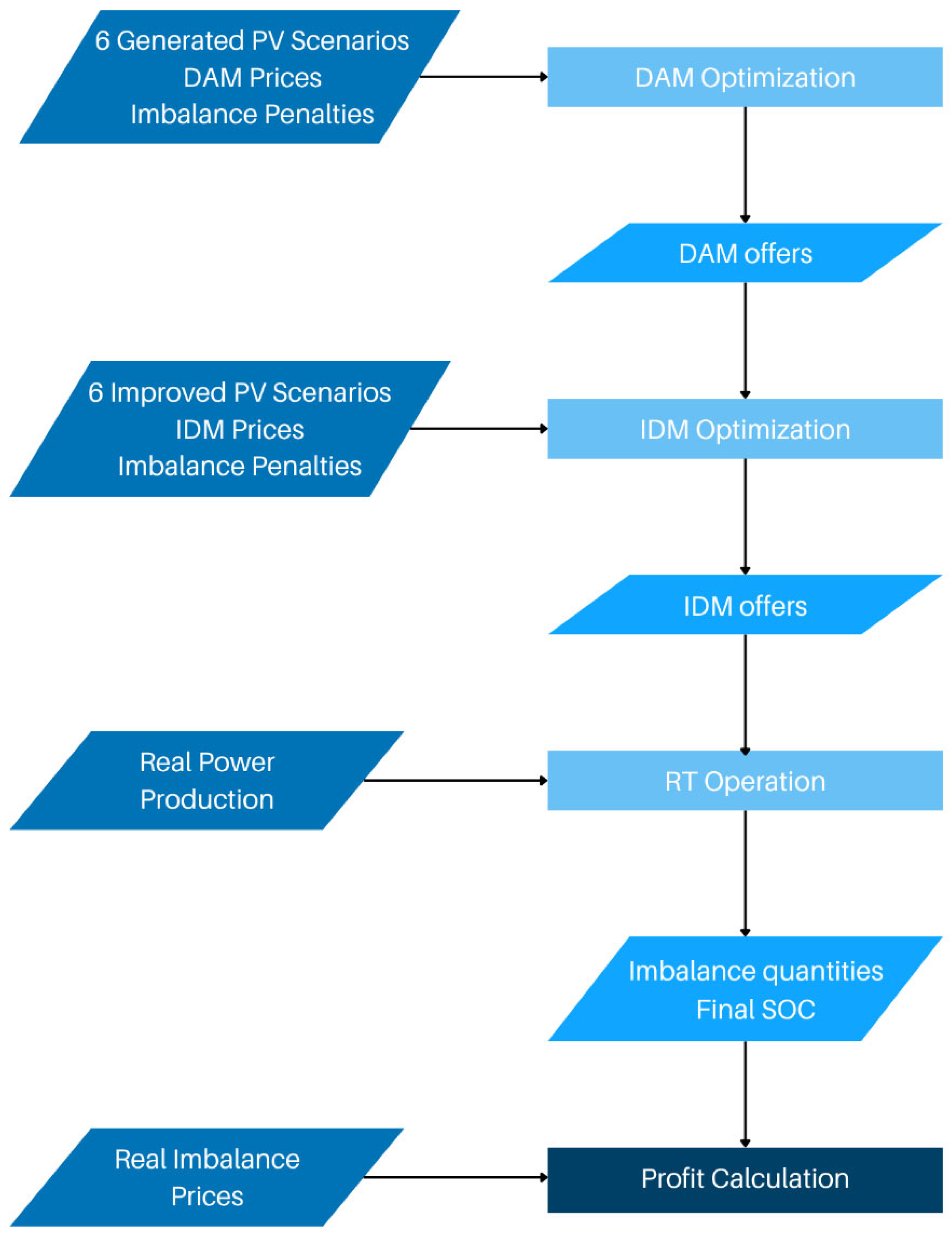
3. Methodology
3.1. PV Scenario Generation
3.1.1. Day-Ahead Market PV Scenarios
- 1.
- Calculation of the average profile of the cluster being analyzed.
- 2.
- Derivation of error profiles as the difference between the various historical profiles and the average profile, with a 15 min resolution.
- 3.
- Application of the Monte Carlo method through a random addition of errors to the average profile. The selected errors must respect the time constraint (an error obtained in a given quarter hour can only be added to the PV production value of the average profile in the same quarter hour) but can belong to different error profiles. The process continues iteratively until the convergence criterion is satisfied.
3.1.2. Intra-Day Market Improved PV Scenarios
3.2. Mathematical Model
3.2.1. Day-Ahead Market
- 1.
- Collection of annual DAM prices and imbalance prices.
- 2.
- Calculation of the difference between imbalance prices and DAM prices over each quarter of an hour of the year.
- 3.
- Computation of the annual average imbalance price deviations for each quarter-hour, separately for negative and positive system imbalances.
- 4.
- Finally, each time a day is simulated, imbalance penalties are computed for each quarter-hour by adding the average imbalance price deviations to the actual daily DAM price profile.
3.2.2. Intra-Day Market
3.2.3. Real-Time Operation
4. Case Studies and Results
4.1. Analyzed Case Studies
- It allows users to specify the exact geographical location of the PV system; in this study, Piazza Leonardo da Vinci in Milan is selected.
- The time period can vary between 2005 and 2024. In this study, the range 2021–2023 is chosen to ensure a comprehensive representation of production profiles.
- The system type can be customized by selecting fixed panels or tracking systems, allowing further customization of tilt and orientation.
- The installed peak power and system losses can be defined.
- 50% of the panels positioned at 0° inclination,
- 25% at 15° inclination,
- 25% at −15° inclination (equivalent tilt but opposite azimuth).
4.2. PV Scenario Generation and Market Data
4.3. Techno-Economic Analysis of PV + BESS Market Participation
4.3.1. Economic Impact of Dispatchability Constraints
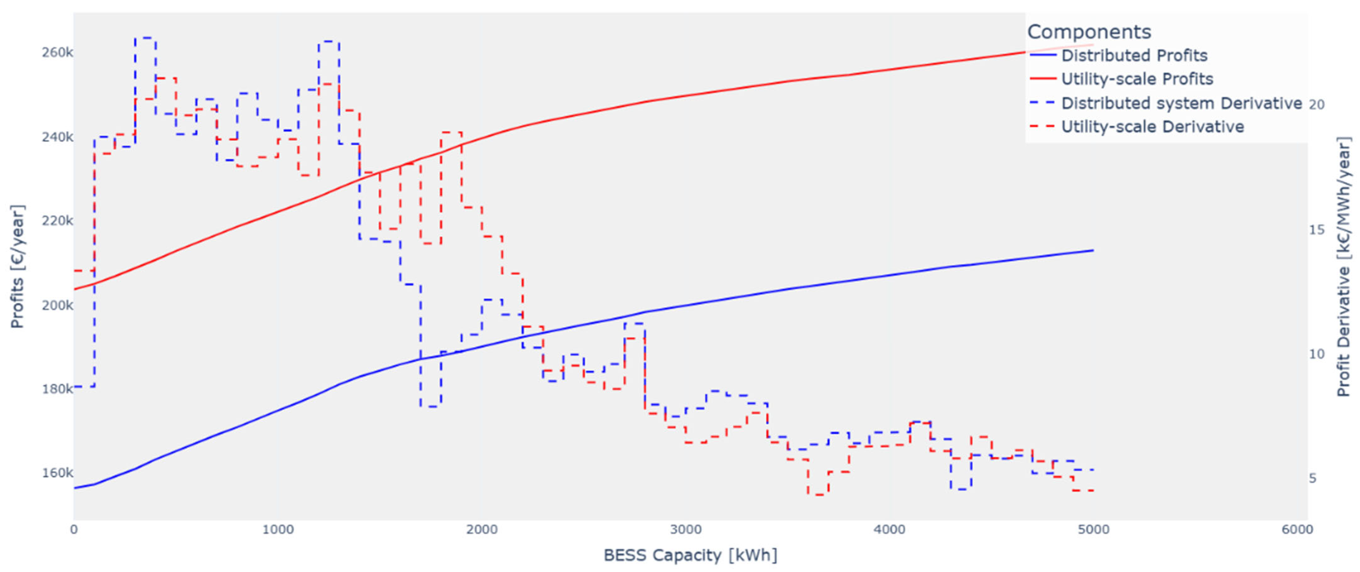
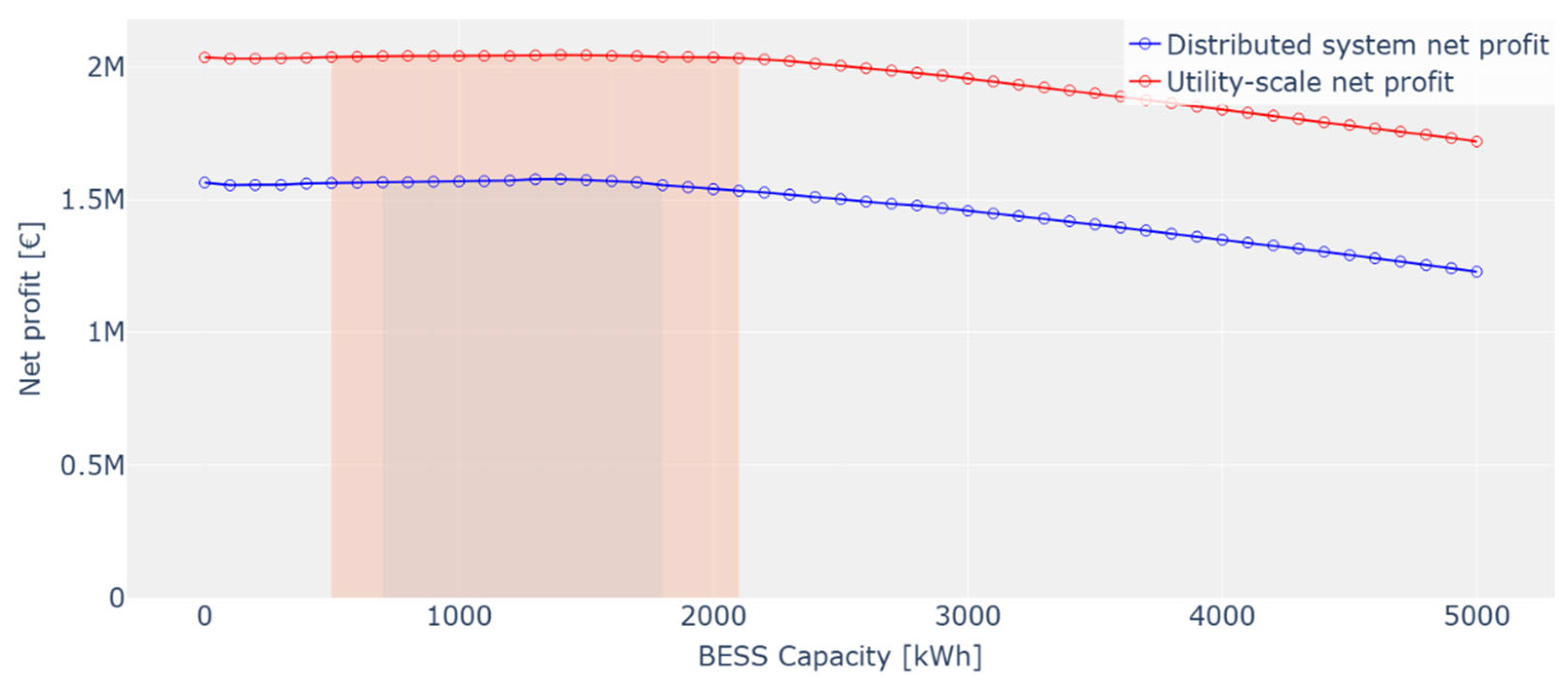
4.3.2. Unconstrained Optimal BESS Sizing
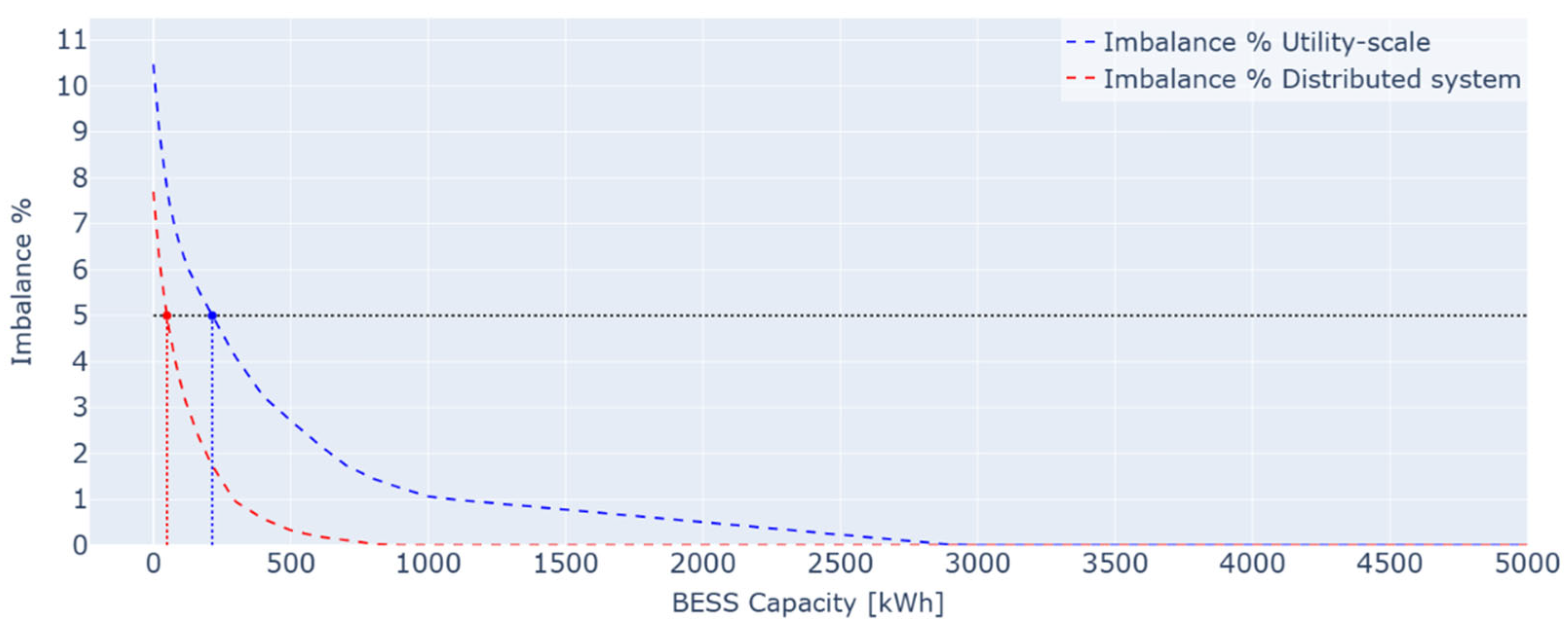
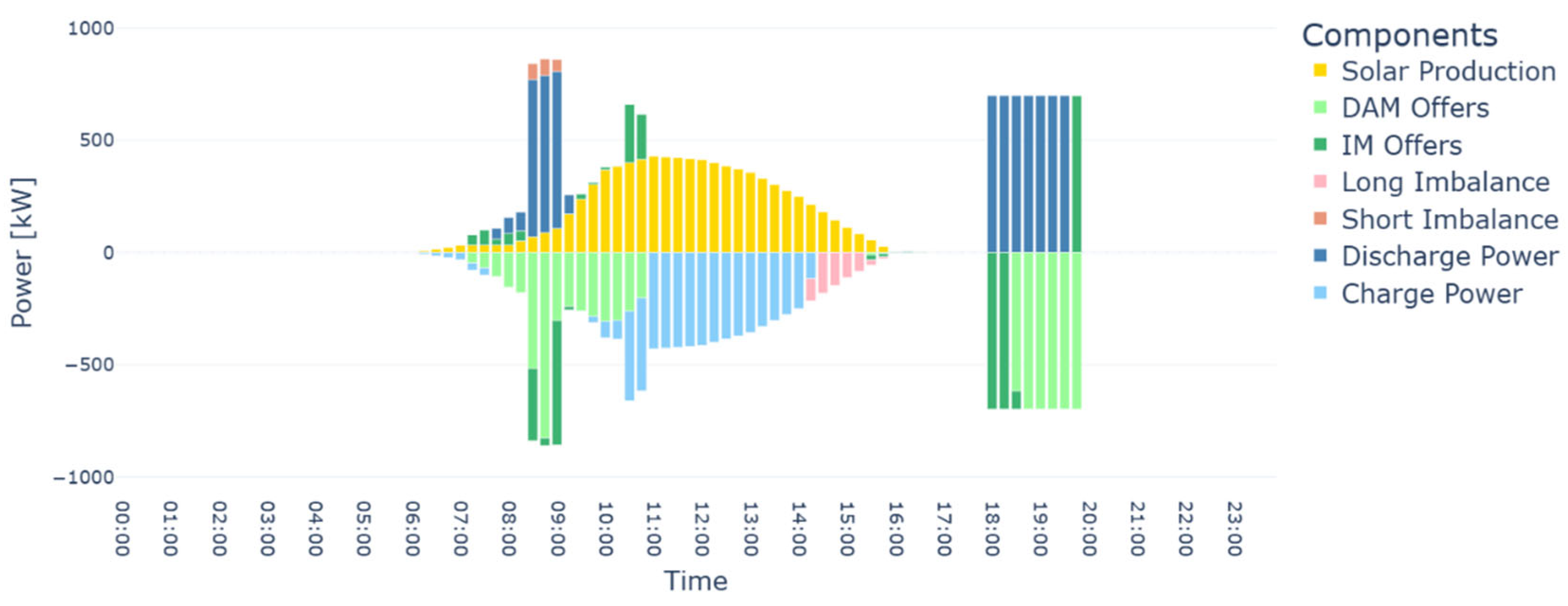
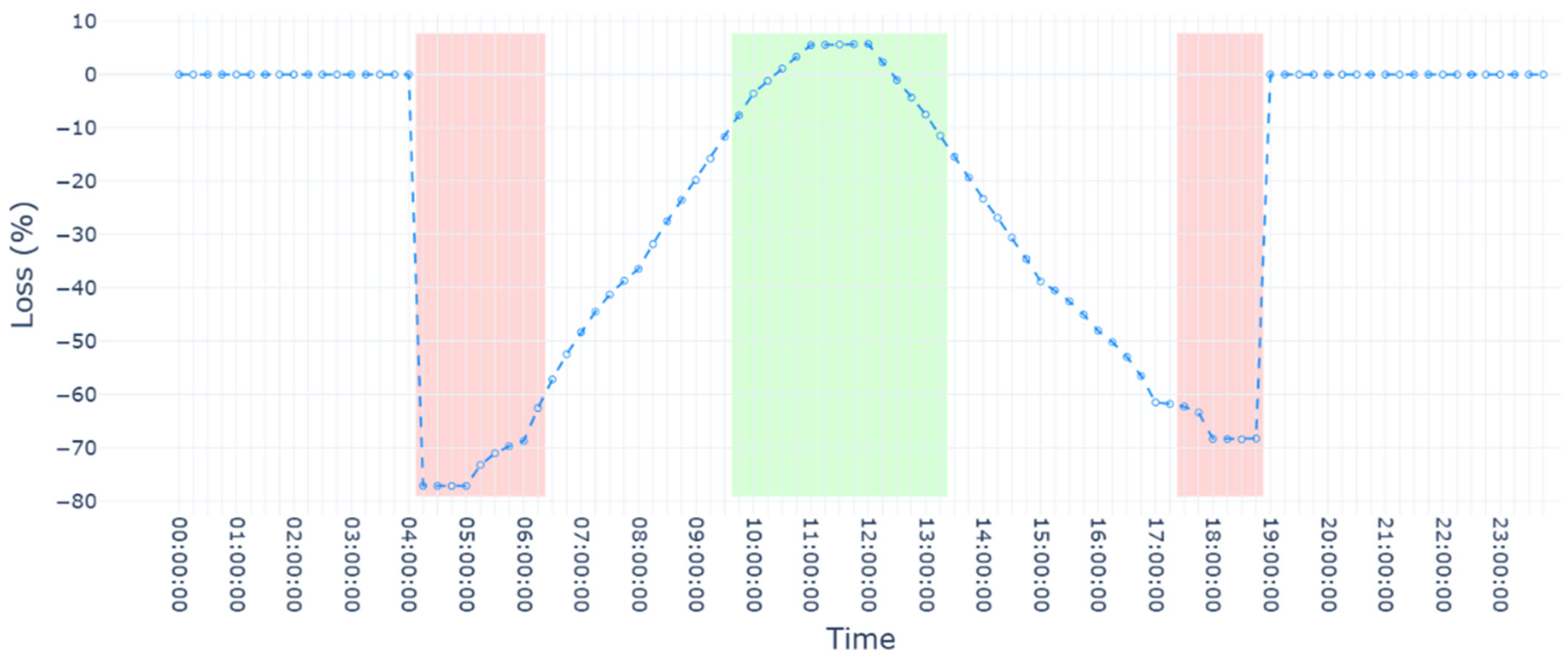
4.3.3. Optimal BESS Sizing Under Dispatchability Constraint
5. Discussion
Author Contributions
Funding
Data Availability Statement
Acknowledgments
Conflicts of Interest
Abbreviations
| ASM | Ancillary Services Market |
| BESS | Battery Energy-Storage System |
| BTM | Behind-The-Meter |
| CF | Capacity Factor |
| CRIDA | Complementary Regional Intra-Day Auction |
| DAM | Day-Ahead Market |
| DER | Distributed Energy Resource |
| EPR | Energy to Power Ratio |
| EU | European Union |
| FTM | Front-of-The-Meter |
| GTC | Gate Time Closure |
| HEMS | Home Energy Management System |
| IDM | Intra-Day Market |
| ISP | Imbalance Settlement Period |
| LCOE | Levelized Cost Of Electricity |
| MILP | Mixed-Integer Linear Programming |
| MTU | Market Time Unit |
| NP-RESs | Non-Programmable Renewable Energy Sources |
| NPV | Net Present Value |
| nRMSE | normalized Root Mean Square Error |
| PV | Photovoltaic |
| PVGIS | Photovoltaic Geographical Information System |
| RESs | Renewable Energy Sources |
| RTP | Real-Time Pricing |
| SOC | State Of Charge |
| SPT | Stepwise Power Tariff |
| TIDE | Testo Integrato del Dispacciamento Elettrico |
| TOU | Time Of Use |
| TSO | Transmission System Operator |
| VPP | Virtual Power Plant |
| UVA | Unità Virtuale Abilitata |
| WCSS | Within-Cluster Sum of Squares |
| XBID | Cross-Border Intra-Day |
Nomenclature
| Sets | Maximum state of charge (%) | ||
| q | Quarter-hour of the day (from 1 to 96) | Charging efficiency (-) | |
| i | Photovoltaic scenario (from 1 to 6) | Discharging efficiency (-) | |
| Parameters | Battery maximum power (MW) | ||
| DAM price at interval q (EUR/MWh) | PV power at interval q in scenario i (MW) | ||
| IDM price at interval q (EUR/MWh) | Variables | ||
| Negative imbalance penalty at interval q (EUR/MWh) | DAM power offer at interval q (MW) | ||
| Positive imbalance penalty at interval q (EUR/MWh) | IDM power offer at interval q (MW) | ||
| Mean DAM price used as reference (EUR/MWh) | Negative imbalance power at interval q in scenario i (MW) | ||
| Real imbalance price (EUR/MWh) | Positive imbalance power at interval q in scenario i (MW) | ||
| Scenario i probability (%) | Charging power at interval q in scenario i (MW) | ||
| Time interval length (h) | Discharging power at interval q in scenario i (MW) | ||
| Initial state of charge (%) | State of charge at interval q in scenario i (%) | ||
| Battery capacity (MWh) | Binary variables defining if the imbalance is negative or positive (-) | ||
| Minimum state of charge (%) | Binary variables defining if the battery is charging or discharging (-) |
Appendix A

| Parameter | Value | Reference |
|---|---|---|
| 55% if BESS power < 15% ; 97.2% otherwise | [52] | |
| 50% if BESS power < 15% ; 86.8% otherwise | [52] | |
| [0, 100, 200, …, 4900, 5000] kWh | [-] | |
| 2 h | [-] | |
| 250 kEUR/MWh | [52] | |
| EUR 80 k/MW | [52] | |
| 100% | [58] | |
| 5 kEUR/MWh/y | [52] | |
| 50% | [-] | |
| 100% | [-] |
| Utility Scale | Distributed System | ||
|---|---|---|---|
| Firming only | BESS size (kWh) | 220 | 50 |
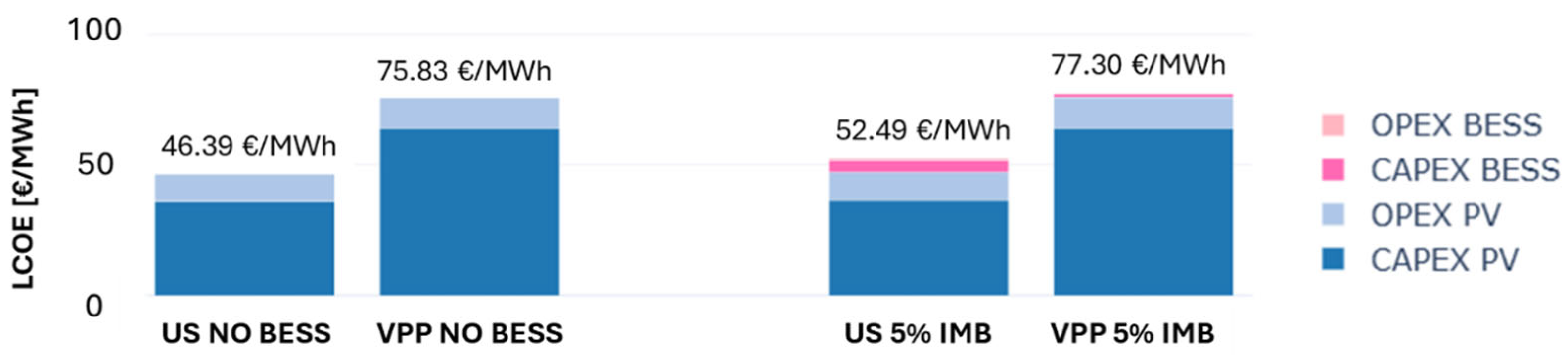
| LCOE (EUR/MWh) | 52.49 (+13.1% vs. PV-only) | 77.30 (+1.94% vs. PV-only) | |
| NPV (k€) | −61 | −20 | |
| Optimal market participation—no imbalance constraint | BESS size (kWh) | 1400 | 1300 |
| LCOE (EUR/MWh) | 86.60 (+86.7% vs. PV-only) | 125.74 (+65.8% vs. PV-only) | |
| NPV (k€) | −239 | −221 | |
| Optimal market participation + firming | BESS size (kWh) | 1700 | 1100 |
| LCOE (EUR/MWh) | 94.53 (+104% vs. PV-only) | 118.94 (+56.9% vs. PV-only) | |
| NPV (k€) | −295 | −191 | |
References
- Greenhouse Gas Emissions from Energy Data Explorer—Data Tools—IEA. Available online: https://www.iea.org/data-and-statistics/data-tools/greenhouse-gas-emissions-from-energy-data-explorer (accessed on 8 May 2025).
- The Paris Agreement|UNFCCC. Available online: https://unfccc.int/process-and-meetings/the-paris-agreement (accessed on 8 May 2025).
- The European Green Deal—European Commission. Available online: https://commission.europa.eu/strategy-and-policy/priorities-2019-2024/european-green-deal_en (accessed on 8 May 2025).
- Global Overview—Renewables 2024—Analysis—IEA. Available online: https://www.iea.org/reports/renewables-2024/global-overview (accessed on 8 May 2025).
- Rosslowe, C.; Petrovich, B. European Electricity Review 2025. 2025. Available online: https://ember-energy.org/app/uploads/2025/01/EER_2025_22012025.pdf (accessed on 28 May 2025).
- SolarPower Europe. EU Market Outlook for Solar Power 2024–2028. Available online: https://www.solarpowereurope.org/insights/outlooks/eu-market-outlook-for-solar-power-2024-2028/detail (accessed on 17 March 2025).
- ARERA. TIDE—Testo Integrato del Dispacciamento Elettrico. Available online: https://www.arera.it/area-operatori/produzione-tide (accessed on 8 May 2025).
- European Parliament. Directive—2019/944—EN—EUR-Lex. Available online: https://eur-lex.europa.eu/eli/dir/2019/944/oj/eng (accessed on 8 May 2025).
- ESO. Balancing Costs: Annual Report and Future Projections. Available online: https://www.neso.energy/document/318666/download (accessed on 28 May 2025).
- European Network of Transmission System Operators for Electricity. Balancing Report 2024. 2024. Available online: https://eepublicdownloads.blob.core.windows.net/public-cdn-container/clean-documents/news/2024/240628_ENTSO-E_Balancing_Report_2024.pdf (accessed on 28 May 2025).
- Saldarini, A.; Longo, M.; Brenna, M.; Zaninelli, D. Battery Electric Storage Systems: Advances, Challenges, and Market Trends. Energies 2023, 16, 7566. [Google Scholar] [CrossRef]
- IEA. Batteries and Secure Energy Transitions. Paris. Available online: https://www.iea.org/reports/batteries-and-secure-energy-transitions (accessed on 28 May 2025).
- Hannan, M.A.; Wali, S.; Ker, P.; Rahman, M.A.; Mansor, M.; Ramachandaramurthy, V.; Muttaqi, K.; Mahlia, T.; Dong, Z. Battery energy-storage system: A review of technologies, optimization objectives, constraints, approaches, and outstanding issues. J. Energy Storage 2021, 42, 103023. [Google Scholar] [CrossRef]
- Niu, D.; Fang, J.; Yau, W.; Goetz, S.M. Comprehensive evaluation of energy storage systems for inertia emulation and frequency regulation improvement. Energy Rep. 2023, 9, 2566–2576. [Google Scholar] [CrossRef]
- Rezaeimozafar, M.; Monaghan, R.F.D.; Barrett, E.; Duffy, M. A review of behind-the-meter energy storage systems in smart grids. Renew. Sustain. Energy Rev. 2022, 164, 112573. [Google Scholar] [CrossRef]
- Zheng, K.; Sun, Z.; Song, Y.; Zhang, C.; Zhang, C.; Chang, F.; Yang, D.; Fu, X. Stochastic Scenario Generation Methods for Uncertainty in Wind and Photovoltaic Power Outputs: A Comprehensive Review. Energies 2025, 18, 503. [Google Scholar] [CrossRef]
- Shi, Q.; Li, F.; Kuruganti, T.; Olama, M.M.; Dong, J.; Wang, X.; Winstead, C. Resilience-Oriented DG Siting and Sizing Considering Stochastic Scenario Reduction. IEEE Trans. Power Syst. 2021, 36, 3715–3727. [Google Scholar] [CrossRef]
- Falabretti, D.; Gulotta, F.; Siface, D. Scheduling and operation of RES-based virtual power plants with e-mobility: A novel integrated stochastic model. Int. J. Electr. Power Energy Syst. 2023, 144, 108604. [Google Scholar] [CrossRef]
- Gabrel, V.; Murat, C.; Thiele, A. Recent advances in robust optimization: An overview. Eur. J. Oper. Res. 2014, 235, 471–483. [Google Scholar] [CrossRef]
- Nemati, H.; Sánchez-Martín, P.; Sigrist, L.; Rouco, L.; Ortega, Á. Flexible robust optimization for Renewable-only VPP bidding on electricity markets with economic risk analysis. Int. J. Electr. Power Energy Syst. 2025, 167, 110594. [Google Scholar] [CrossRef]
- Silva, A.R.; Pousinho, H.M.I.; Estanqueiro, A. A multistage stochastic approach for the optimal bidding of variable renewable energy in the day-ahead, intraday and balancing markets. Energy 2022, 258, 124856. [Google Scholar] [CrossRef]
- Visser, L.R.; AlSkaif, T.A.; Khurram, A.; Kleissl, J.; van Sark, W.G.H.J.M. Probabilistic solar power forecasting: An economic and technical evaluation of an optimal market bidding strategy. Appl. Energy 2024, 370, 123573. [Google Scholar] [CrossRef]
- Rancilio, G.; Dimovski, A.; Bovera, F.; Moncecchi, M.; Falabretti, D.; Merlo, M. Service stacking on residential BESS: RES integration by flexibility provision on ancillary services markets. Sustain. Energy Grids Netw. 2023, 35, 101097. [Google Scholar] [CrossRef]
- Li, J. Optimal sizing of grid-connected photovoltaic battery systems for residential houses in Australia. Renew. Energy 2019, 136, 1245–1254. [Google Scholar] [CrossRef]
- Duman, A.C.; Erden, H.S.; Gönül, Ö.; Güler, Ö. Optimal sizing of PV-BESS units for home energy management system-equipped households considering day-ahead load scheduling for demand response and self-consumption. Energy Build. 2022, 267, 112164. [Google Scholar] [CrossRef]
- Zhou, L.; Zhang, Y.; Lin, X.; Li, C.; Cai, Z.; Yang, P. Optimal sizing of PV and bess for a smart household considering different price mechanisms. IEEE Access 2018, 6, 41050–41059. [Google Scholar] [CrossRef]
- DICOPT. Available online: https://www.gams.com/latest/docs/S_DICOPT.html (accessed on 24 May 2025).
- Rezaeimozafar, M.; Duffy, M.; Monaghan, R.F.D.; Barrett, E. Residential PV-battery scheduling with stochastic optimization and neural network-driven scenario generation. Energy Rep. 2024, 12, 418–429. [Google Scholar] [CrossRef]
- Guo, Y.; Gong, Y.; Fang, Y.; Khargonekar, P.P. Stochastic minimization of imbalance cost for a virtual power plant in electricity markets. In Proceedings of the 2014 IEEE PES Innovative Smart Grid Technologies Conference, ISGT 2014, Washington, DC, USA, 19–22 February 2014. [Google Scholar] [CrossRef]
- Marneris, I.G.; Ntomaris, A.V.; Biskas, P.N.; Baslis, C.G.; Chatzigiannis, D.I.; Demoulias, C.S.; Oureilidis, K.O.; Bakirtzis, A.G. Optimal Participation of RES Aggregators in Energy and Ancillary Services Markets. IEEE Trans. Ind. Appl. 2023, 59, 232–243. [Google Scholar] [CrossRef]
- Pierro, M.; Perez, R.; Perez, M.; Moser, D.; Cornaro, C. Italian protocol for massive solar integration: Imbalance mitigation strategies. Renew. Energy 2020, 153, 725–739. [Google Scholar] [CrossRef]
- Pierro, M.; Perez, R.; Perez, M.; Prina, M.G.; Moser, D.; Cornaro, C. Italian protocol for massive solar integration: From solar imbalance regulation to firm 24/365 solar generation. Renew. Energy 2021, 169, 425–436. [Google Scholar] [CrossRef]
- Pierro, M.; Perez, R.; Perez, M.; Moser, D.; Cornaro, C. Imbalance mitigation strategy via flexible PV ancillary services: The Italian case study. Renew. Energy 2021, 179, 1694–1705. [Google Scholar] [CrossRef]
- Lazard 2023 Levelized Cost of Energy + Report|Lazard. Available online: https://www.lazard.com/research-insights/2023-levelized-cost-of-energyplus/ (accessed on 9 June 2025).
- CAISO. Home | California ISO. Available online: https://www.caiso.com/ (accessed on 9 June 2025).
- Renewable Energy Progress Tracker—Data Tools—IEA. Available online: https://www.iea.org/data-and-statistics/data-tools/renewable-energy-progress-tracker (accessed on 7 May 2025).
- Pyomo. Available online: https://www.pyomo.org/ (accessed on 24 May 2025).
- Gurobi Optimization. Available online: https://www.gurobi.com/ (accessed on 24 May 2025).
- Politecnico di Milano. PoliGrid—A Smart Grid in Piazza Leonardo. Available online: https://www.polimi.it/en/sustainable-development/environment/energy-and-decarbonisation/energy-committee/translate-to-english-poligrid (accessed on 9 May 2025).
- European Commission. Photovoltaic Geographical Information System (PVGIS). Available online: https://joint-research-centre.ec.europa.eu/photovoltaic-geographical-information-system-pvgis_en (accessed on 9 May 2025).
- Regulation—2017/2195—EN—EUR-Lex. Available online: https://eur-lex.europa.eu/eli/reg/2017/2195/oj/eng (accessed on 9 May 2025).
- GME. Spot Market (MPE). Available online: https://www.mercatoelettrico.org/en-us/Home/Markets/ElectricityMarket/Spot-Market-MPE (accessed on 9 May 2025).
- GME. Vademecum to the Italian Power Exchange. Available online: https://www.mercatoelettrico.org/Portals/0/Documents/en-us/20250101VademecumBorsaElettrica_En.pdf (accessed on 9 May 2025).
- ARERA. Delibera 19 Marzo 2019 103/2019/R/eel. Available online: https://www.arera.it/atti-e-provvedimenti/dettaglio/19/103-19 (accessed on 27 June 2025).
- ARERA. Delibera 23 Novembre 2021 523/2021/R/eel. Available online: https://www.arera.it/atti-e-provvedimenti/dettaglio/21/523-21 (accessed on 9 May 2025).
- Scrocca, A.; Andreotti, D.; Spiller, M.; Rancilio, G.; Bovera, F.; Delfanti, M. Impact of Dynamic Imbalance Pricing on Electricity Market Operators in Italy. In Proceedings of the 2025 21st International Conference on the European Energy Market (EEM), Lisbon, Portugal, 27–29 May 2025; pp. 1–8. [Google Scholar] [CrossRef]
- Abud, T.P.; Augusto, A.A.; Fortes, M.Z.; Maciel, R.S.; Borba, B.S.M.C. State of the Art Monte Carlo Method Applied to Power System Analysis with Distributed Generation. Energies 2023, 16, 394. [Google Scholar] [CrossRef]
- Voyant, C.; Notton, G.; Kalogirou, S.; Nivet, M.-L.; Paoli, C.; Motte, F.; Fouilloy, A. Machine learning methods for solar radiation forecasting: A review. Renew. Energy 2017, 105, 569–582. [Google Scholar] [CrossRef]
- Benali, L.; Notton, G.; Fouilloy, A.; Voyant, C.; Dizene, R. Solar radiation forecasting using artificial neural network and random forest methods: Application to normal beam, horizontal diffuse and global components. Renew. Energy 2019, 132, 871–884. [Google Scholar] [CrossRef]
- Krishnan, N.; Kumar, K.R.; Inda, C.S. How solar radiation forecasting impacts the utilization of solar energy: A critical review. J. Clean. Prod. 2023, 388, 135860. [Google Scholar] [CrossRef]
- Lago, J.; Marcjasz, G.; De Schutter, B.; Weron, R. Forecasting day-ahead electricity prices: A review of state-of-the-art algorithms, best practices and an open-access benchmark. Appl. Energy 2021, 293, 116983. [Google Scholar] [CrossRef]
- Scrocca, A.; Bovera, F.; Rancilio, G.; Delfanti, M.; Zatti, M. Techno-Economic Optimization of Services Stacking for a Battery Participating to Electricity Spot Markets. In Proceedings of the International Conference on the European Energy Market, EEM, Istanbul, Turkiye, 10–12 June 2024. [Google Scholar] [CrossRef]
- Vandewetering, N.; Jamil, U.; Pearce, J.M. Ballast-Supported Foundation Designs for Low-Cost Open-Source Solar Photovoltaic Racking. Designs 2024, 8, 17. [Google Scholar] [CrossRef]
- Barbón, A.; Martínez-Suárez, J.; Bayón, L.; Bayón-Cueli, C. Photovoltaic Power Plants with Horizontal Single-Axis Trackers: Influence of the Movement Limit on Incident Solar Irradiance. Appl. Sci. 2025, 15, 1175. [Google Scholar] [CrossRef]
- Omoyele, O.; Hoffmann, M.; Koivisto, M.; Larrañeta, M.; Weinand, J.M.; Linßen, J.; Stolten, D. Increasing the resolution of solar and wind time series for energy system modeling: A review. Renew. Sustain. Energy Rev. 2024, 189, 113792. [Google Scholar] [CrossRef]
- GME. Esiti Elettricità. Available online: https://gme.mercatoelettrico.org/it-it/Home/Esiti/Elettricita/MGP/Esiti/PUN (accessed on 22 May 2025).
- Terna. SunSet—Area Pubblica. Available online: https://myterna.terna.it/SunSet/Public (accessed on 22 May 2025).
- IRENA. Electricity Storage and Renewables: Costs and Markets to 2030; International Renewable Energy Agency: Masdar City, Abu Dhabi, 2017; 132p, Available online: https://www.irena.org/-/media/Files/IRENA/Agency/Publication/2017/Oct/IRENA_Electricity_Storage_Costs_2017.pdf (accessed on 30 June 2025).
- Home|NREL. Available online: https://www.nrel.gov/ (accessed on 22 May 2025).
- Naemi, M.; Davis, D.; Brear, M.J. Optimisation and analysis of battery storage integrated into a wind power plant participating in a wholesale electricity market with energy and ancillary services. J. Clean. Prod. 2022, 373, 133909. [Google Scholar] [CrossRef]
- Mohamed, A.; Rigo-Mariani, R.; Debusschere, V.; Pin, L. Stacked revenues for energy storage participating in energy and reserve markets with an optimal frequency regulation modeling. Appl. Energy 2023, 350, 121721. [Google Scholar] [CrossRef]
- Andreotti, D.; Spiller, M.; Scrocca, A.; Bovera, F.; Rancilio, G. Modeling and Analysis of BESS Operations in Electricity Markets: Prediction and Strategies for Day-Ahead and Continuous Intra-Day Markets. Sustainability 2024, 16, 7940. [Google Scholar] [CrossRef]
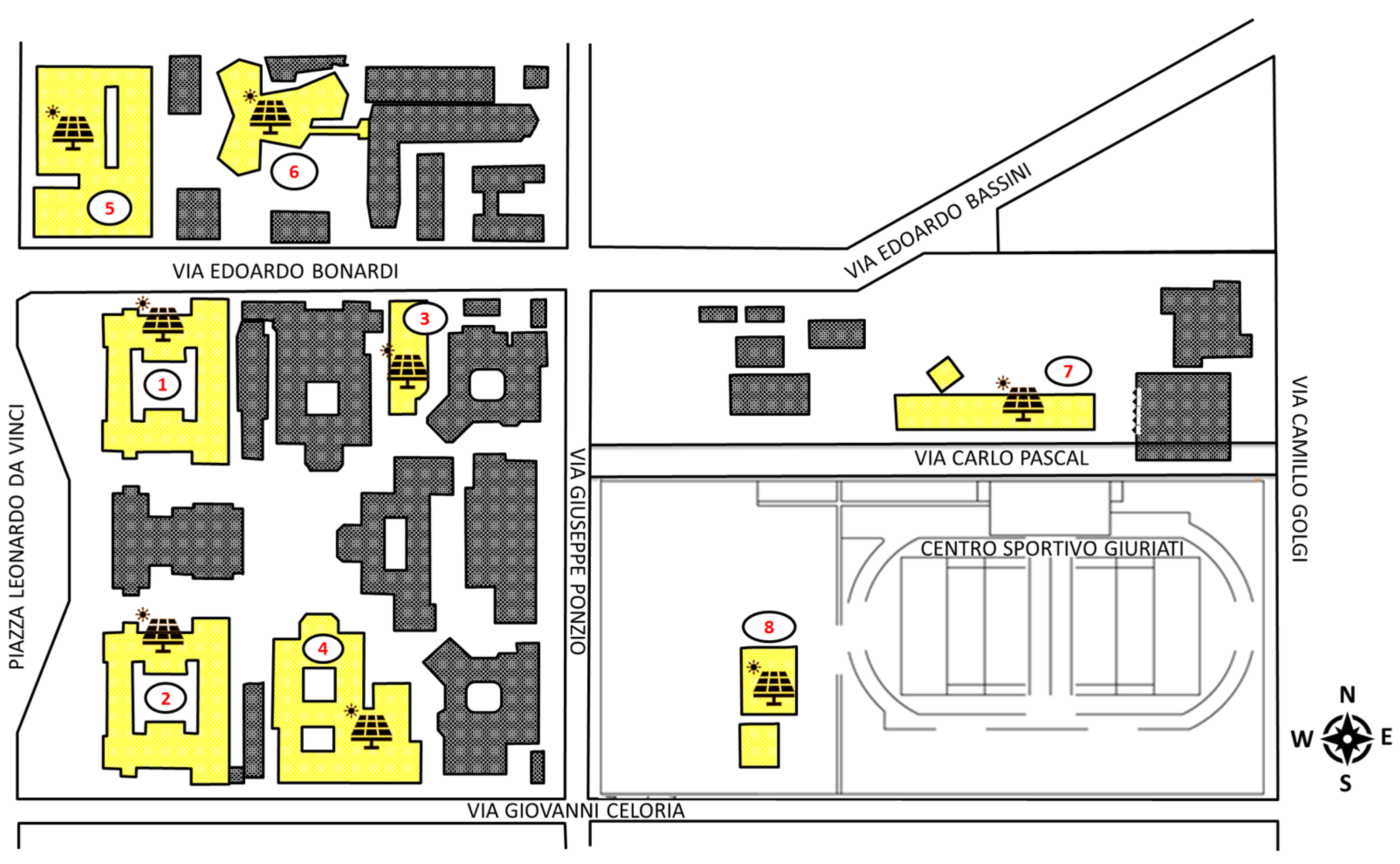


| Power Plant | Type | Peak Power (kW) | Losses (%) | Tilt (°) | Azimuth (°) |
|---|---|---|---|---|---|
| 1 | Rooftop—Coplanar | 199.30 | 12.85 | 6 | 90 |
| 2 | Rooftop—Coplanar | 165.56 | 12.43 | 9 | 90 |
| 3 | Rooftop—Barrel shaped | 84.36 | 12.57 | 0 | 90 |
| 42.18 | 12.57 | 15 | 90 | ||
| 42.18 | 12.57 | −15 | −90 | ||
| 4 | Rooftop—Coplanar | 46.40 | 13.73 | 15 | 0 |
| 13.59 | 19.90 | 27 | 0 | ||
| 0.62 | 17.72 | 15.9 | 90 | ||
| 5 | Rooftop—Coplanar | 139.19 | 12.95 | 15.9 | 90 |
| 6 | Flat Roof—Ballasted | 50.22 | 13.74 | 9 | −15 |
| 50.22 | 13.74 | 9 | −168.46 | ||
| 54.72 | 13.74 | 9 | 80 | ||
| 7 | Rooftop—Coplanar | 82.25 | 11.71 | 10 | 0 |
| 8 | Flat Roof—Ballasted | 29.53 | 11.43 | 30 | 0 |
| Season | Sunny Weather | Variable Weather | Cloudy Weather |
|---|---|---|---|
| Winter | 1 March 2023 | 24 January 2023 | 21 December 2023 |
| Spring | 6 May 2023 | 29 April 2023 | 30 March 2023 |
| Summer | 20 July 2023 | 23 August 2023 | 15 September 2023 |
| Autumn | 3 October 2023 | 31 October 2023 | 26 October 2023 |
| Season | Cluster | Occurrence Probability Utility-Scale (%) | Occurrence Probability Distributed System (%) |
|---|---|---|---|
| Winter | Sunny | 6.94 | 7.95 |
| Variable | 9.04 | 9.50 | |
| Cloudy | 8.67 | 7.21 | |
| Spring | Sunny | 15.07 | 16.26 |
| Variable | 5.39 | 6.12 | |
| Cloudy | 4.75 | 2.83 | |
| Summer | Sunny | 10.59 | 11.69 |
| Variable | 10.41 | 9.41 | |
| Cloudy | 4.20 | 4.11 | |
| Autumn | Sunny | 6.03 | 6.58 |
| Variable | 9.86 | 9.86 | |
| Cloudy | 9.04 | 8.50 |
Disclaimer/Publisher’s Note: The statements, opinions and data contained in all publications are solely those of the individual author(s) and contributor(s) and not of MDPI and/or the editor(s). MDPI and/or the editor(s) disclaim responsibility for any injury to people or property resulting from any ideas, methods, instructions or products referred to in the content. |
© 2025 by the authors. Licensee MDPI, Basel, Switzerland. This article is an open access article distributed under the terms and conditions of the Creative Commons Attribution (CC BY) license (https://creativecommons.org/licenses/by/4.0/).
Share and Cite
Scrocca, A.; Pisani, R.; Andreotti, D.; Rancilio, G.; Delfanti, M.; Bovera, F. Optimal Spot Market Participation of PV + BESS: Impact of BESS Sizing in Utility-Scale and Distributed Configurations. Energies 2025, 18, 3791. https://doi.org/10.3390/en18143791
Scrocca A, Pisani R, Andreotti D, Rancilio G, Delfanti M, Bovera F. Optimal Spot Market Participation of PV + BESS: Impact of BESS Sizing in Utility-Scale and Distributed Configurations. Energies. 2025; 18(14):3791. https://doi.org/10.3390/en18143791
Chicago/Turabian StyleScrocca, Andrea, Roberto Pisani, Diego Andreotti, Giuliano Rancilio, Maurizio Delfanti, and Filippo Bovera. 2025. "Optimal Spot Market Participation of PV + BESS: Impact of BESS Sizing in Utility-Scale and Distributed Configurations" Energies 18, no. 14: 3791. https://doi.org/10.3390/en18143791
APA StyleScrocca, A., Pisani, R., Andreotti, D., Rancilio, G., Delfanti, M., & Bovera, F. (2025). Optimal Spot Market Participation of PV + BESS: Impact of BESS Sizing in Utility-Scale and Distributed Configurations. Energies, 18(14), 3791. https://doi.org/10.3390/en18143791