

Optimization of Electric Transformer Operation Through Load Estimation Based on the K-Means Algorithm

 ,
,  , ,
, , 
Abstract
1. Introduction
1.1. Context
1.2. Related Works
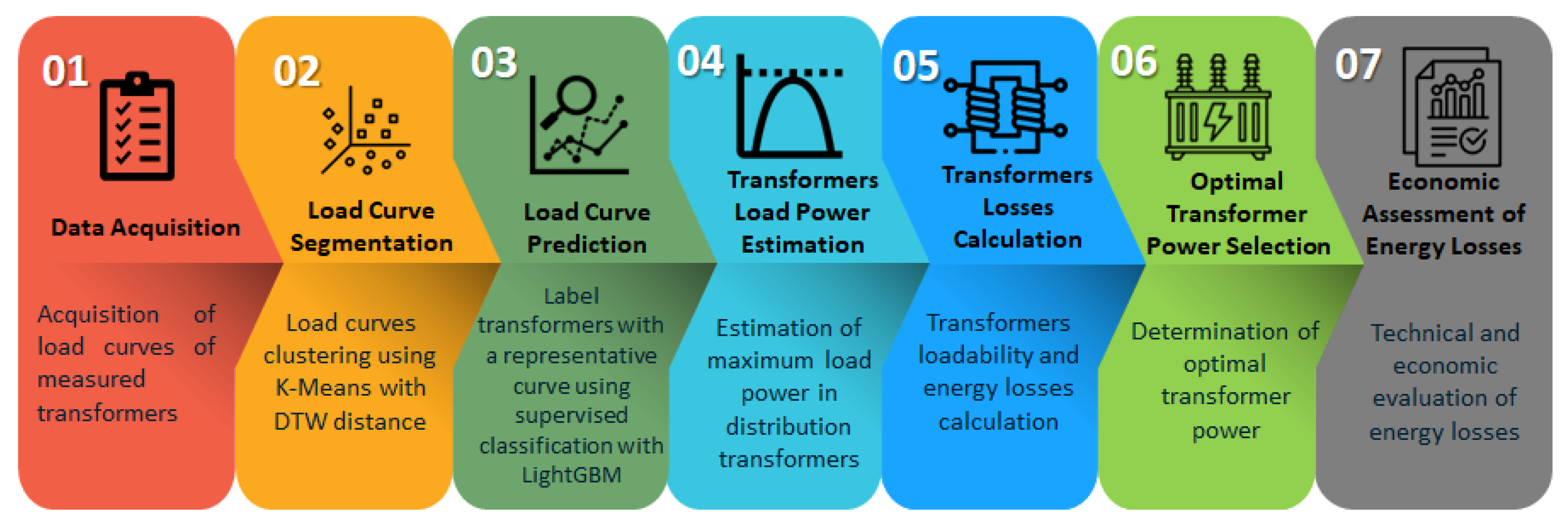
2. Materials and Methods
2.1. Data Acquisition
2.2. Load Curve Segmentation
2.3. Load Curve Prediction
2.4. Estimation of Maximum Load Power in Distribution Transformers
2.5. Transformer Losses Calculation
2.5.1. Technical Losses in Distribution Transformers
2.5.2. Transformer No-Load Loss Energy
2.5.3. Transformer Load Loss Energy
2.5.4. Total Annual Energy Losses
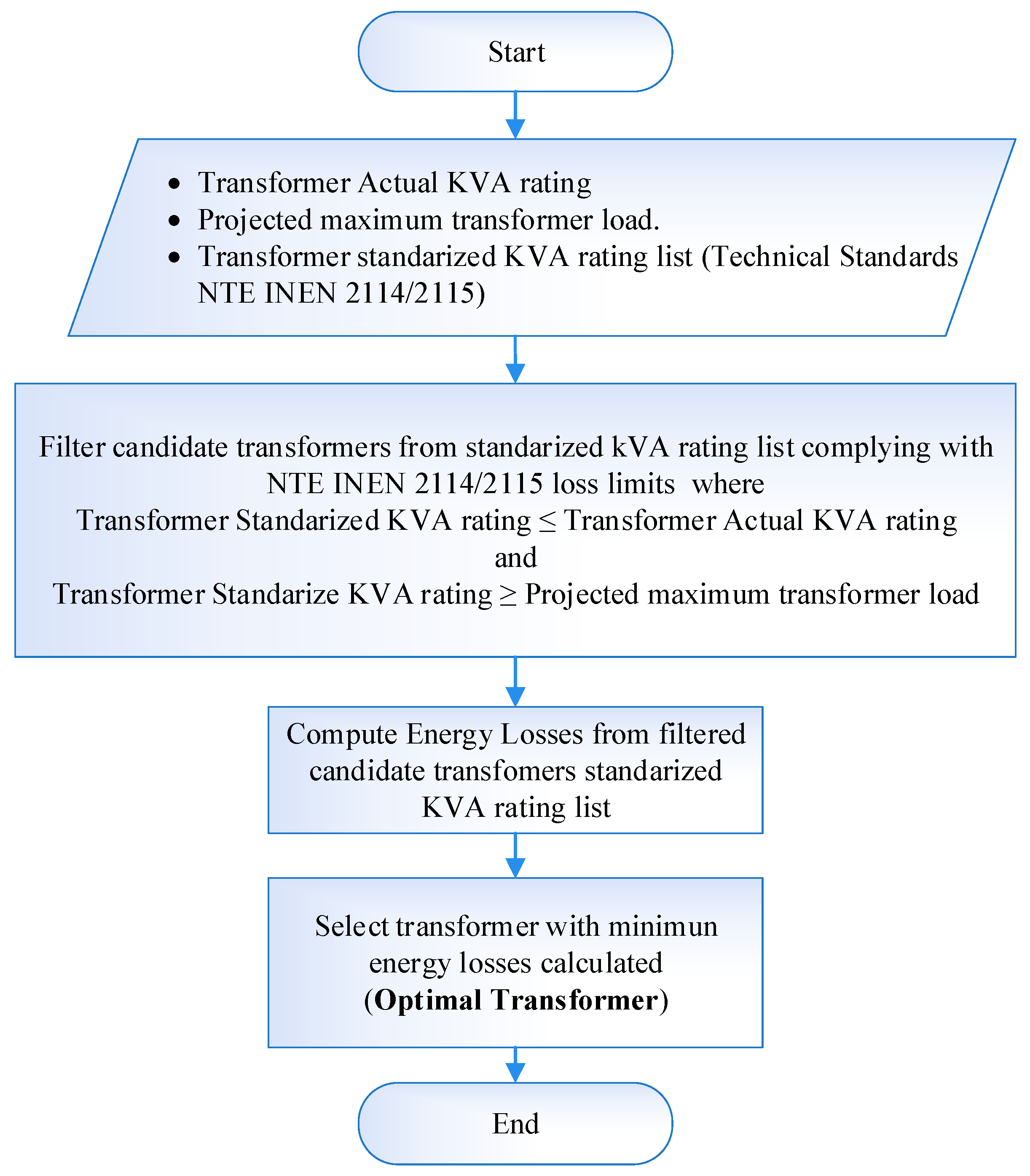
2.6. Selection of the Optimal Transformer
2.7. Economic Assessment of Energy Losses
3. Results and Discussion
3.1. Characteristic Load Curves
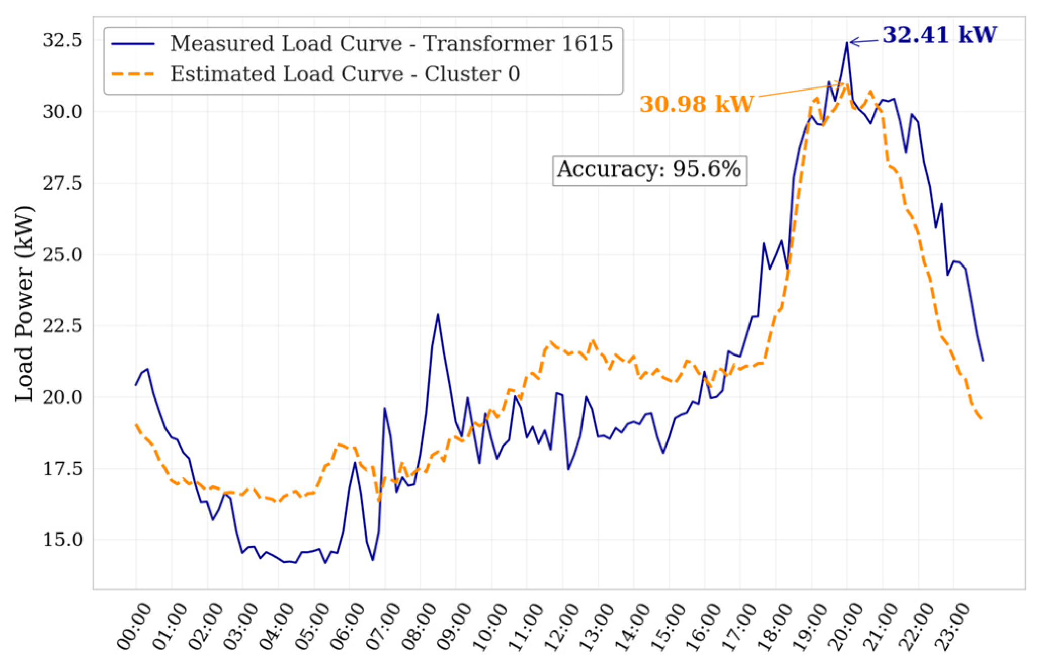
3.2. Transformer Load Curve Prediction
3.3. Transformer Peak Load Determination and Metodology Validation
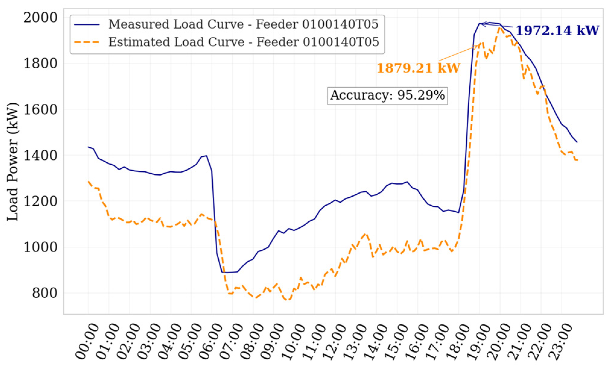
3.3.1. Evaluation on a Complete Feeder
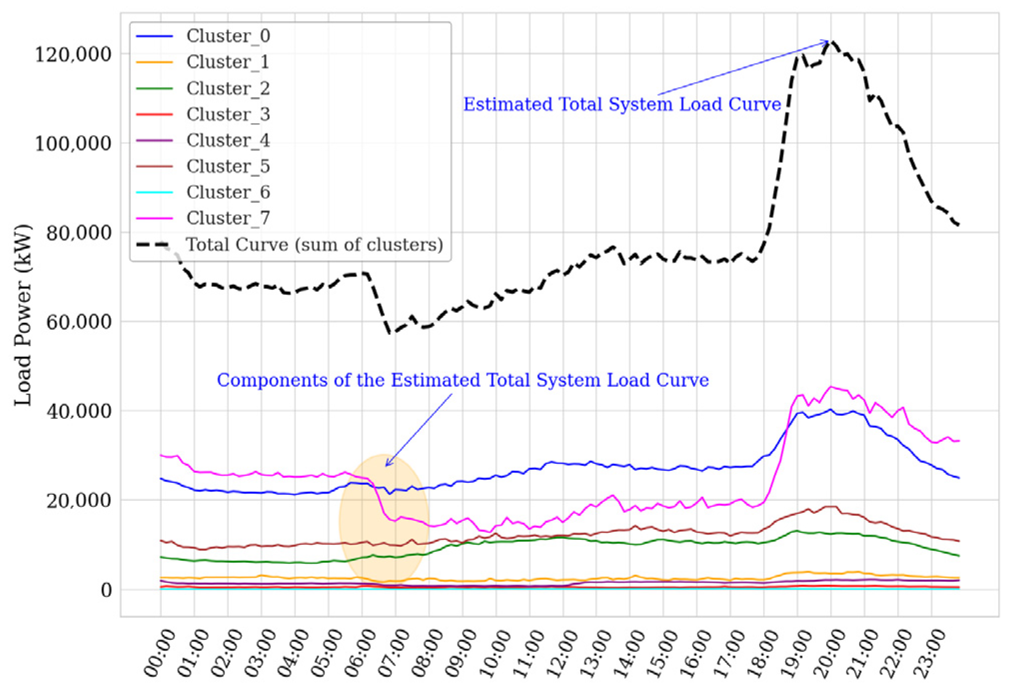
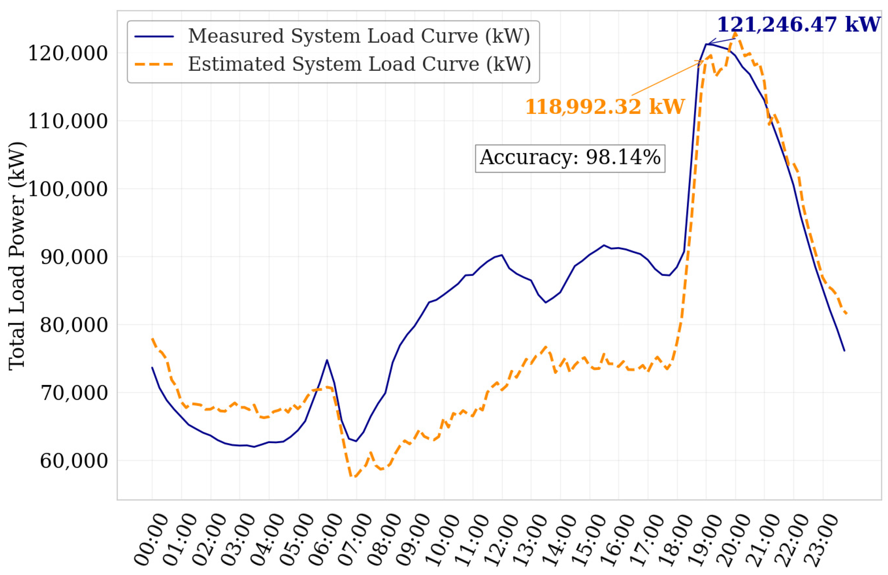
3.3.2. Generalization, Evaluation on a Complete Electrical System
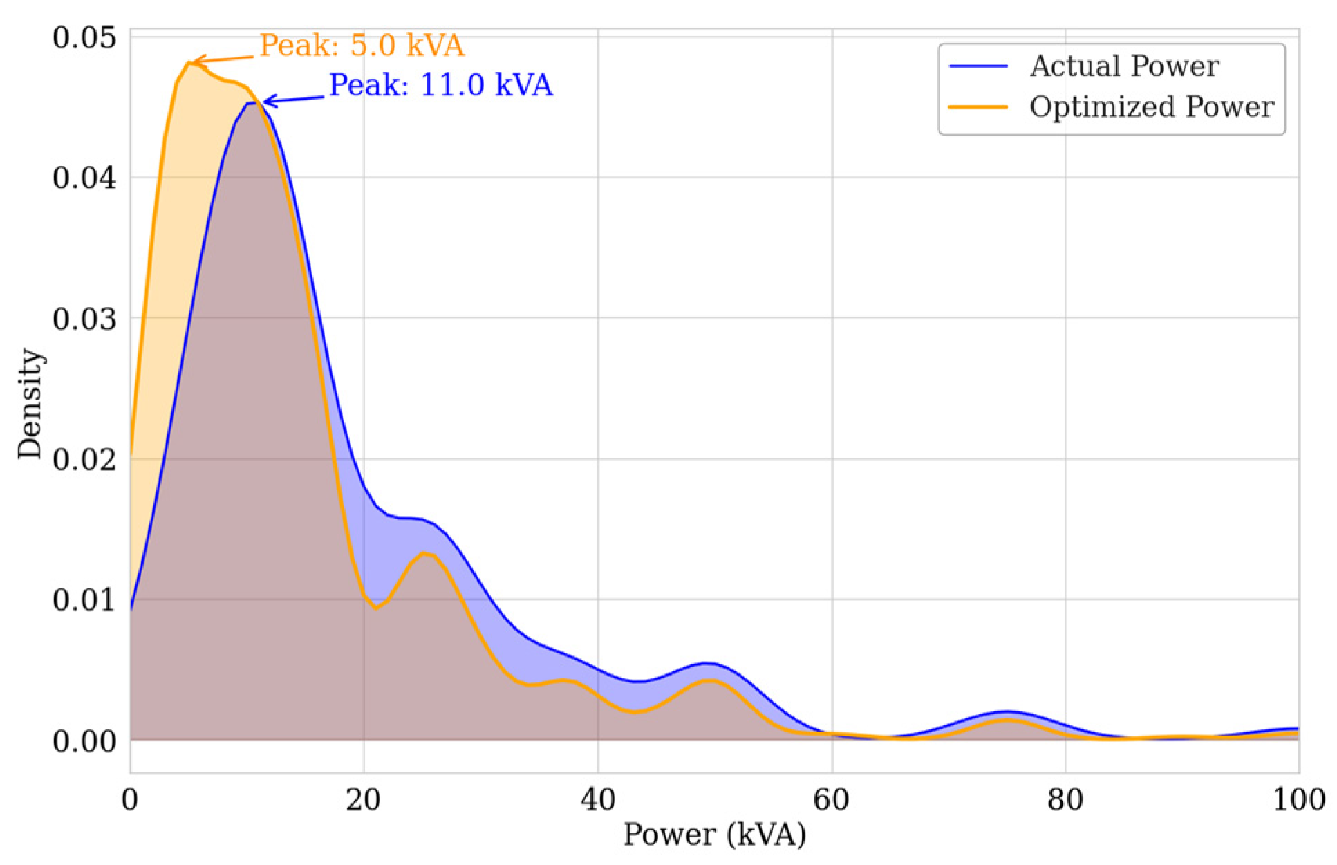
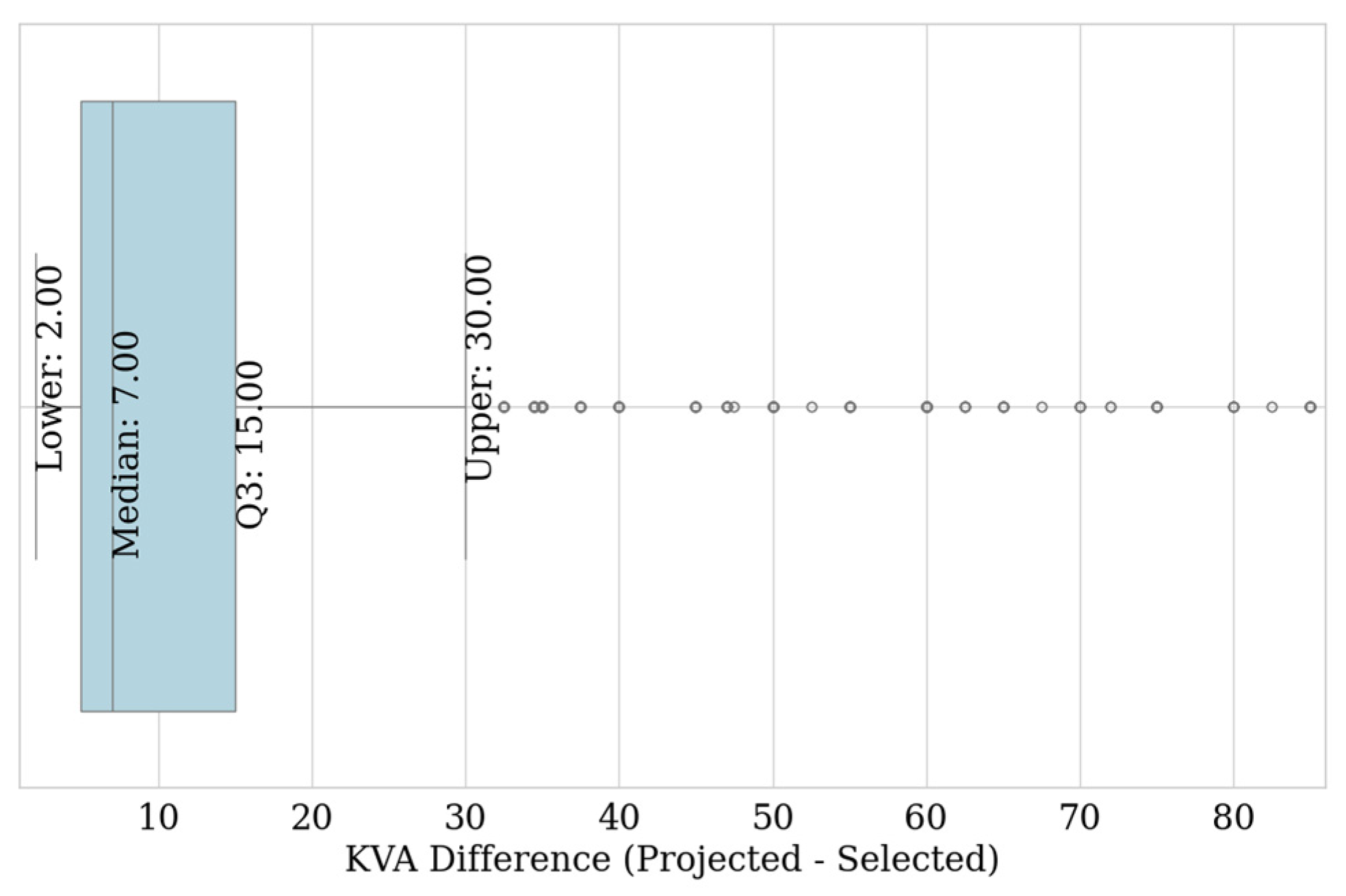
3.4. Determination of Optimal Transformer Power
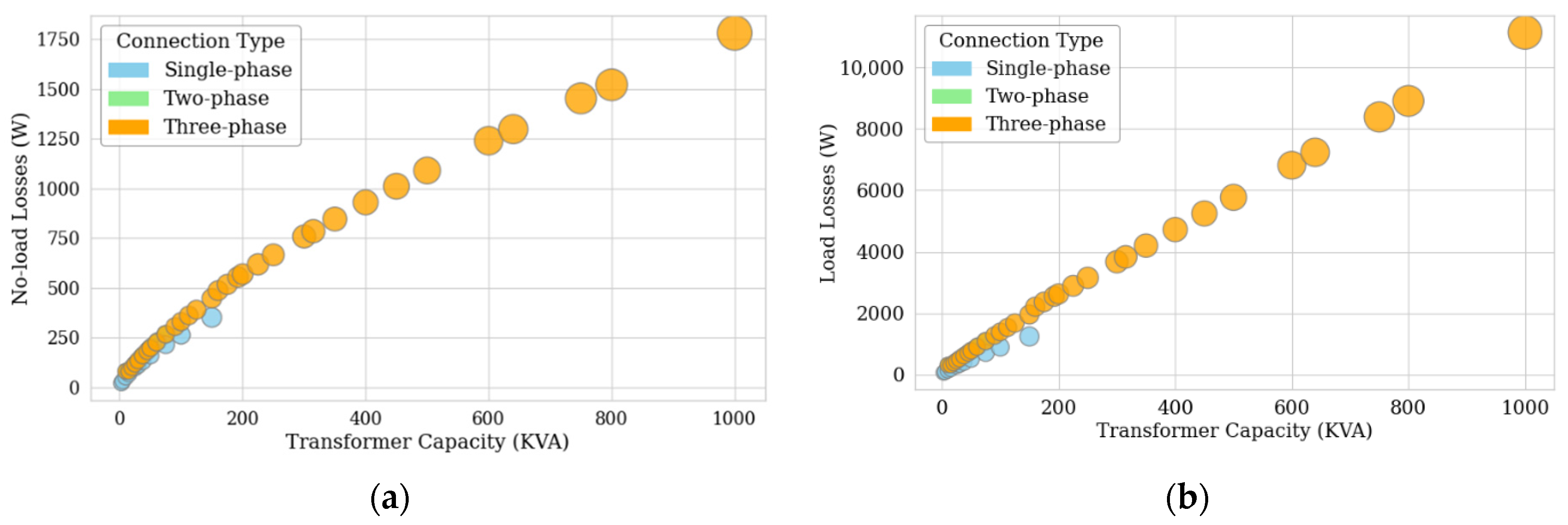
3.5. Evaluation of No-Load and Load Losses in Distribution Transformers
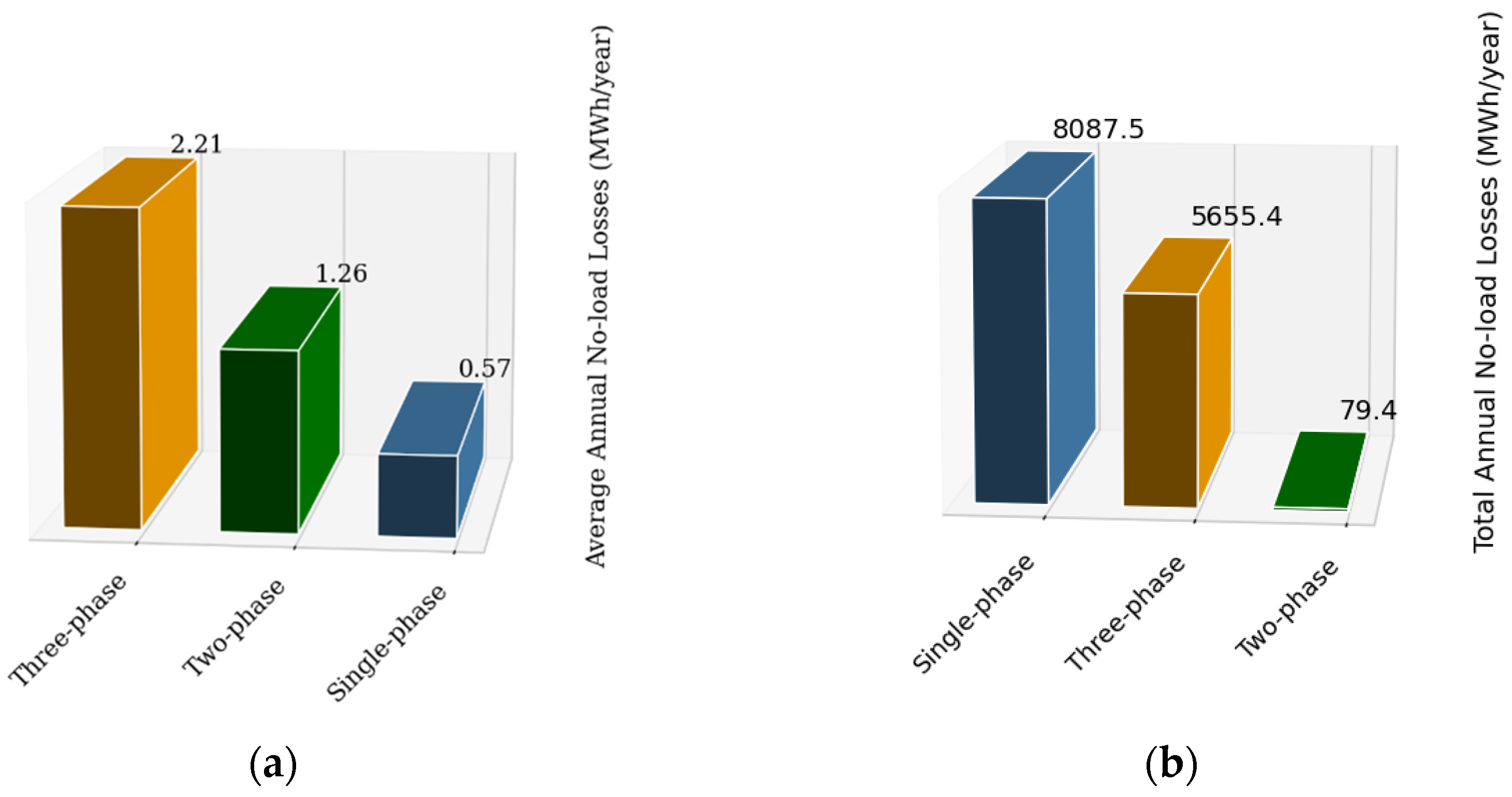
3.5.1. Results of the Evaluation of No-Load Losses in Distribution Transformers
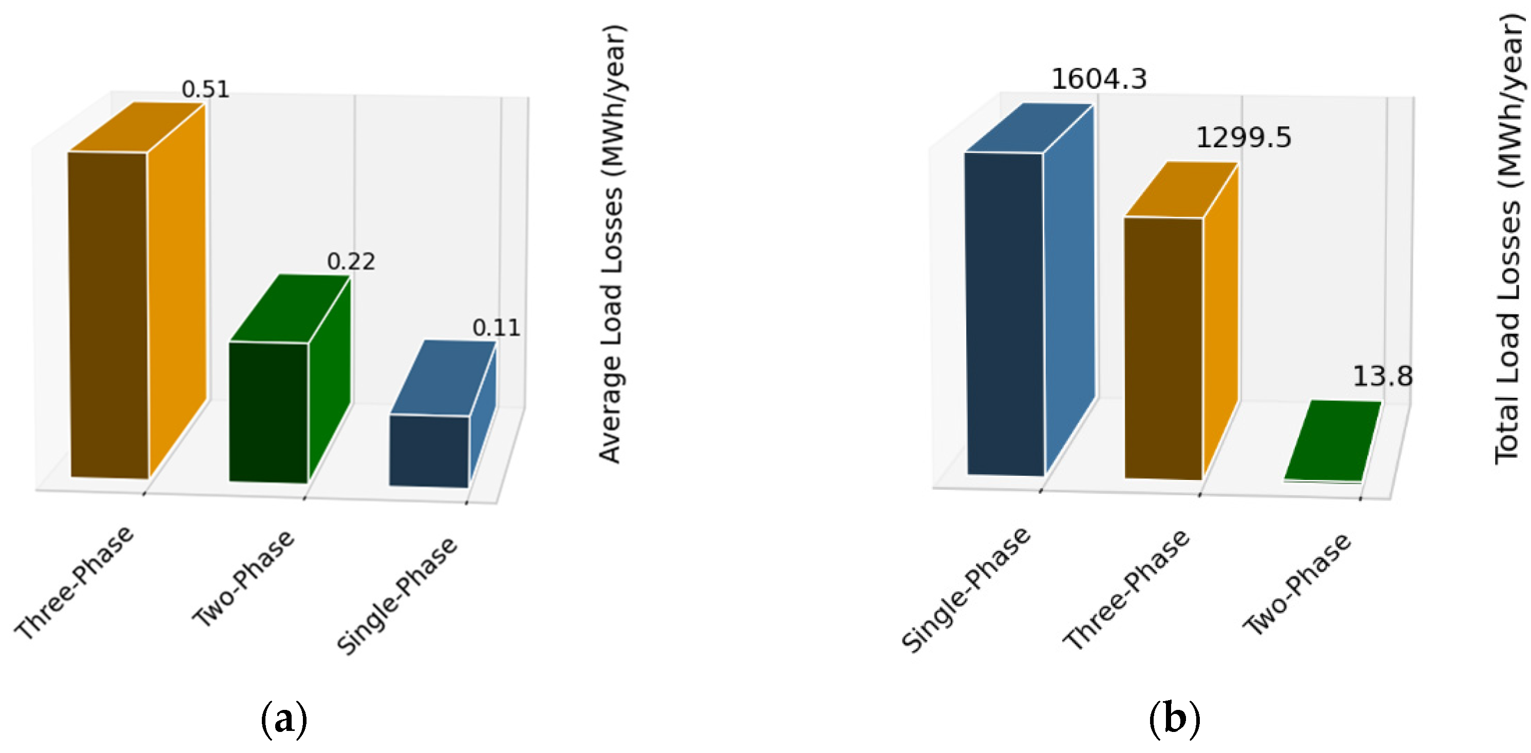
3.5.2. Results of the Evaluation of Load Losses in Distribution Transformers
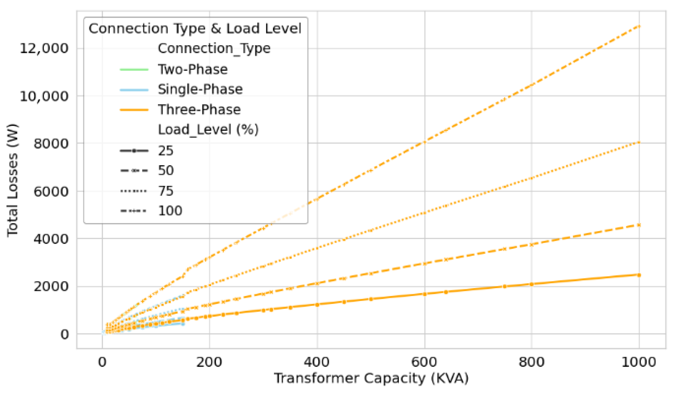
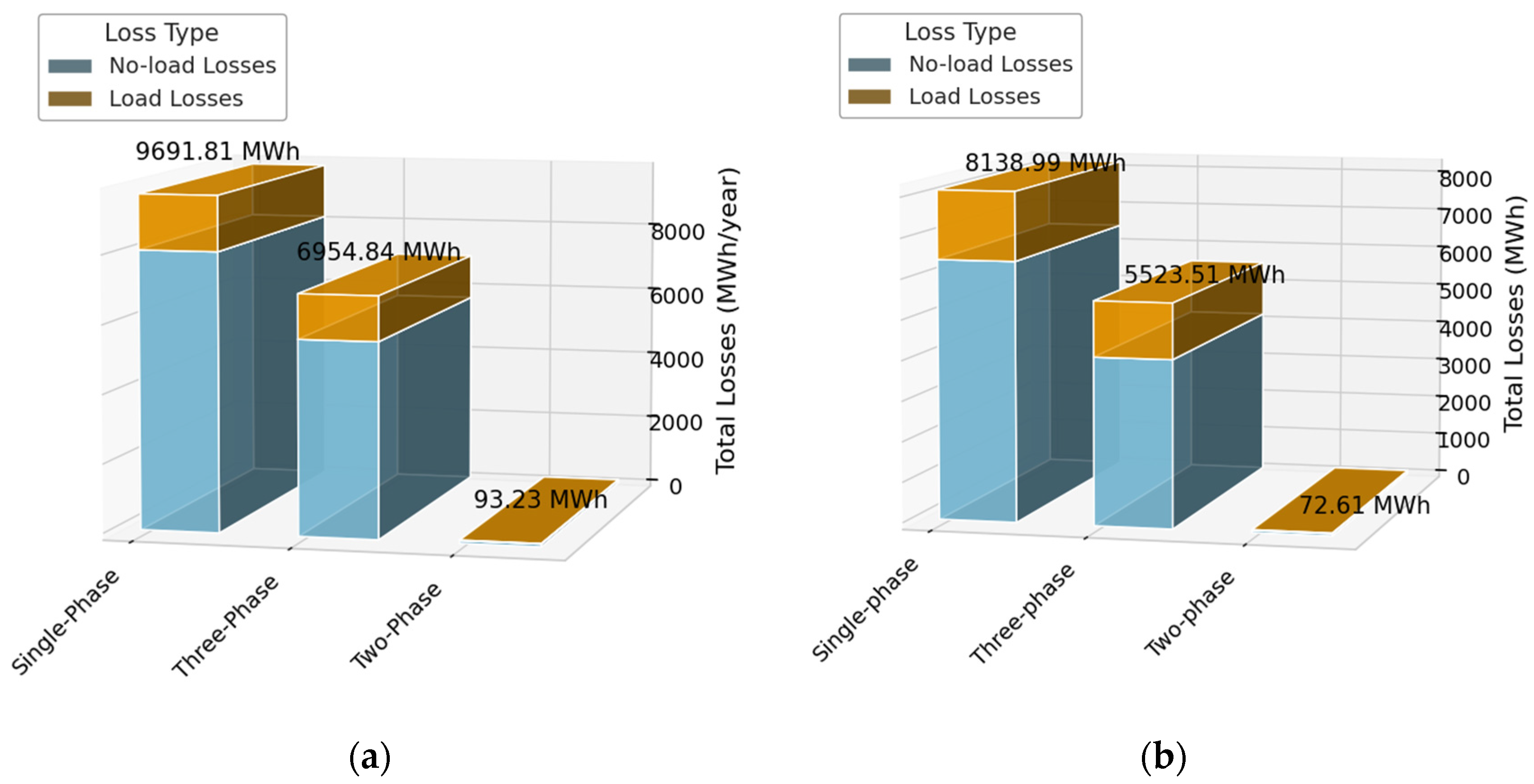
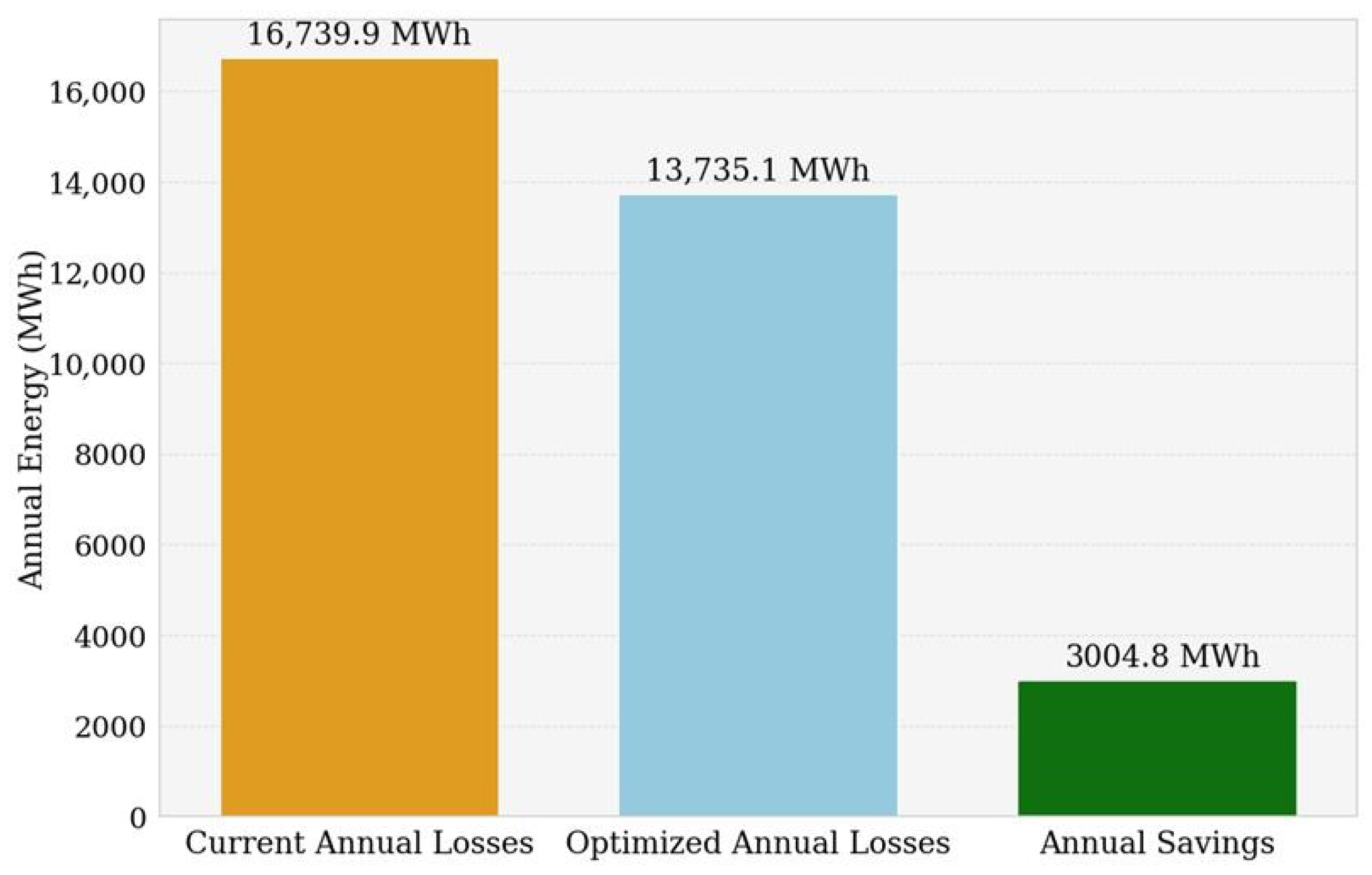
3.5.3. Evaluation of Total Energy Losses in Existing and Optimized Distribution Transformers
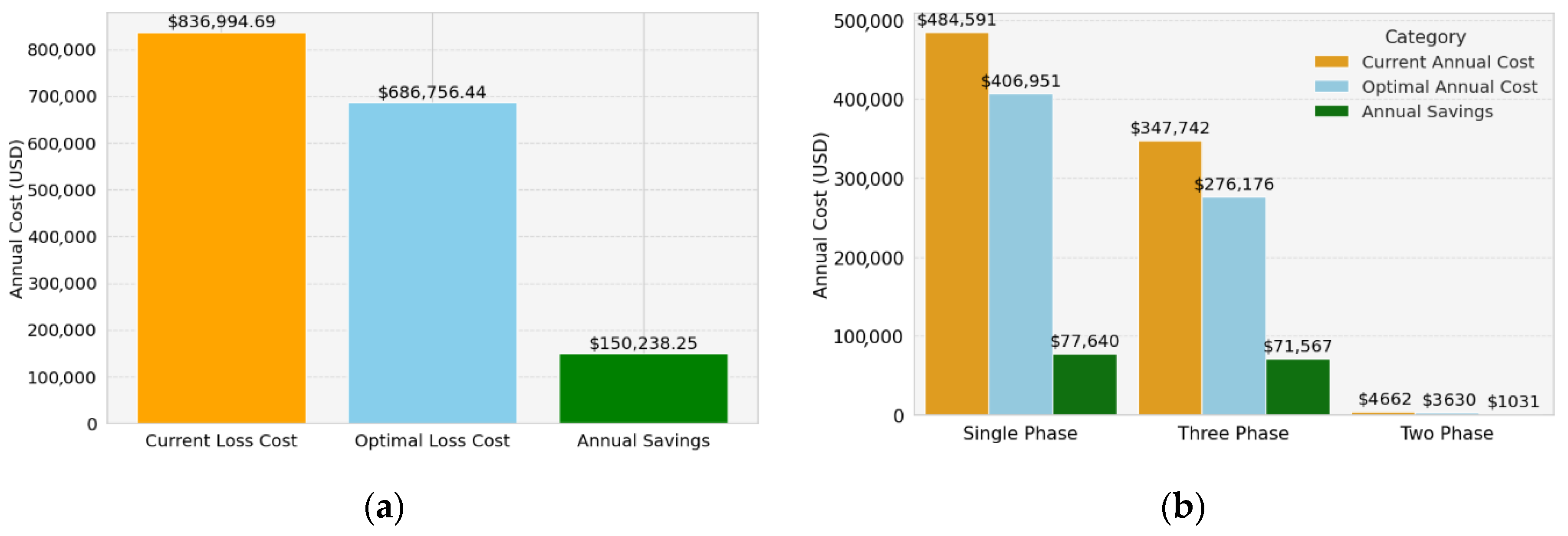
3.6. Economic Evaluation of Energy Losses
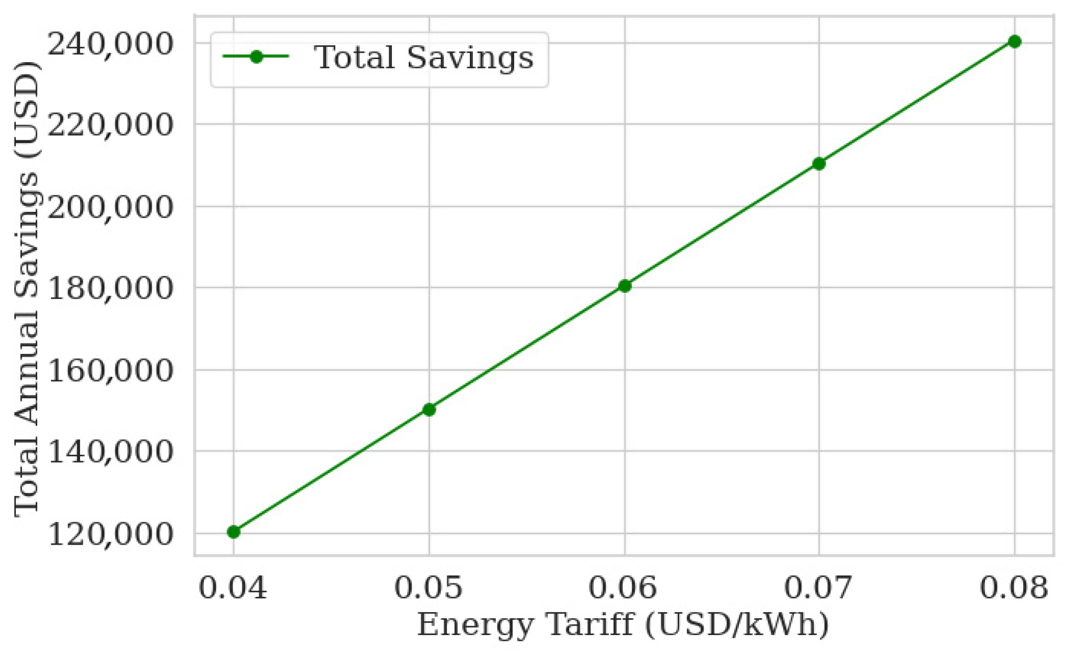
Sensitivity Analysis of Economic Savings to Energy Price Variations
4. Conclusions
Author Contributions
Funding
Data Availability Statement
Acknowledgments
Conflicts of Interest
References
- Amoiralis, E.I.; Tsili, M.A.; Kladas, A.G. Economic evaluation of transformer selection in electrical power systems. In Proceedings of the 19th International Conference on Electrical Machines, ICEM 2010, Rome, Italy, 6–8 September 2010. [Google Scholar] [CrossRef]
- Güldürek, M.; Esenboğa, B. Assessment of Corporate Carbon Footprint and Energy Analysis of Transformer Industry. Sustainability 2024, 16, 5800. [Google Scholar] [CrossRef]
- Piotrowski, T.; Markowska, D. Carbon Footprint of Power Transformers Evaluated Through Life Cycle Analysis. Energies 2025, 18, 1373. [Google Scholar] [CrossRef]
- Agha, A. Economic Evaluation of Transformer Selection in Distribution Systems. 2018. Available online: https://www.researchgate.net/publication/340133579 (accessed on 5 April 2025).
- León-Martínez, V.; Peñalvo-López, E.; Montañana-Romeu, J.; Andrada-Monrós, C.; Molina-Cañamero, L. Assessment of Load Losses Caused by Harmonic Currents in Distribution Transformers Using the Transformer Loss Calculator Software. Environments 2023, 10, 177. [Google Scholar] [CrossRef]
- Wijayapala, W.D.A.S.; Gamage, S.R.K.; Bandara, H.M.S.L.G. Determination of Capitalization Values for No Load Loss and Load Loss in Distribution Transformers. Eng. J. Inst. Eng. Sri Lanka 2016, 49, 11. [Google Scholar] [CrossRef]
- Al-Badi, A.H.; Elmoudi, A.; Metwally, I.; Al-Wahaibi, A.; Al-Ajmi, H.; Al Bulushi, M. Losses reduction in distribution transformers. In Proceedings of the International MultiConference of Engineers and Computer Scientists, Hong Kong, China, 16–18 March 2011; Available online: https://www.iaeng.org/publication/IMECS2011/IMECS2011_pp948-952.pdf (accessed on 15 June 2025).
- Wang, X.; Guo, Q.; Tu, C.; Li, J.; Xiao, F.; Wan, D. A two-stage optimal strategy for flexible interconnection distribution network considering the loss characteristic of key equipment. Int. J. Electr. Power Energy Syst. 2023, 152, 109232. [Google Scholar] [CrossRef]
- Cabral, T.W.; Fraidenraich, G.; Meloni, L.G.P.; Neto, F.B.; de Lima, E.R. Analysis of Variance Combined with Optimized Gradient Boosting Machines for Enhanced Load Recognition in Home Energy Management Systems. Sensors 2024, 24, 4965. [Google Scholar] [CrossRef] [PubMed]
- Torres-Bermeo, P.; López-Eugenio, K.; Varela-Aldás, J.; Del-Valle-Soto, C.; Palacios-Navarro, G. Sizing and Characterization of Load Curves of Distribution Transformers Using Clustering and Predictive Machine Learning Models. Energies 2025, 18, 1832. [Google Scholar] [CrossRef]
- Agudelo, L.; Velilla, E.; López, J.M. Load estimation of power transformers using an artificial neural network|Estimación de la carga de transformadores de potencia utilizando una red neuronal artificial. Inf. Tecnol. 2014, 25, 15–23. [Google Scholar] [CrossRef]
- Chen, Y.; Ye, Y.; Liu, J.; Zhang, L.; Li, W.; Mohtaram, S. Machine Learning Approach to Predict Building Thermal Load Considering Feature Variable Dimensions: An Office Building Case Study. Buildings 2023, 13, 312. [Google Scholar] [CrossRef]
- Mulliez, E.; Sanz-Bobi, M.A.; Sanchez, Á.; Mazidi, P.; González, A.; Bachiller, R. Life characterization of power distribution transformers using clustering techniques. In Proceedings of the European Conference of the Prognostics and Health Management Society, Utrecht, The Netherlands, 3–6 July 2018; Volume 3, pp. 1–7. [Google Scholar]
- Yuan, S.; Zhang, X.; Geng, J.; Wan, D. Research on load curve clustering of distribution transformer based on wavelet transform and big data processing. In Proceedings of the 2017 IEEE 2nd Information Technology, Networking, Electronic and Automation Control Conference, ITNEC 2017, Chengdu, China, 15–17 December 2017; pp. 348–351. [Google Scholar] [CrossRef]
- Zhao, J.; He, J.; Wang, J.; Liu, K. Energy Consumption Prediction for Electric Buses Based on Traction Modeling and LightGBM. World Electr. Veh. J. 2025, 16, 159. [Google Scholar] [CrossRef]
- Hajiaghapour-Moghimi, M.; Azimi-Hosseini, K.; Hajipour, E.; Vakilian, M. Residential Load Clustering Contribution to Accurate Distribution Transformer Sizing. In Proceedings of the 34th International Power System Conference, PSC 2019, Tehran, Iran, 9–11 December 2019; pp. 313–319. [Google Scholar] [CrossRef]
- Téllez, A.A.; Robayo, A.; Ortiz, L.; López, G.; Isaac, I.; González, J. Optimal sizing of distribution transformers using exhaustive search algorithm. In Proceedings of the 2019 Fise IEEE Cigre Conference Living the Energy Transition Fise Cigre 2019, Medellin, Colombia, 4–6 December 2019. [Google Scholar] [CrossRef]
- Agha, A.; Attar, H.; Luhach, A.K. Optimized Economic Loading of Distribution Transformers Using Minimum Energy Loss Computing. Math. Probl. Eng. 2021, 2021, 8081212. [Google Scholar] [CrossRef]
- Biçen, Y.; Aras, F.; Kirkici, H. Lifetime estimation and monitoring of power transformer considering annual load factors. IEEE Trans. Dielectr. Electr. Insul. 2014, 21, 1360–1367. [Google Scholar] [CrossRef]
- Mendoza, J.E.; López, M.E.; Peña, H.E.; Labra, D.A. Low voltage distribution optimization: Site, quantity and size of distribution transformers. Electr. Power Syst. Res. 2012, 91, 52–60. [Google Scholar] [CrossRef]
- Li, Y.; Han, G.; Yue, S.; Wan, Z.; Yin, J. Structure design and magnetic-vibration characteristics analysis of hybrid core for high efficiency distribution transformer. AIP Adv. 2025, 15, 035041. [Google Scholar] [CrossRef]
- Schröder, K.; Farias, G.; Dormido-Canto, S.; Fabregas, E. Comparative Analysis of Deep Learning Methods for Fault Avoidance and Predicting Demand in Electrical Distribution. Energies 2024, 17, 2709. [Google Scholar] [CrossRef]
- Farahzad, K.; Shahbahrami, A.; Ashouri, M. Optimal Capacity Determination for Electrical Distribution Transformers Based On IEC 60076-7 And Practical Load Data. Int. J. Eng. Manuf. 2020, 10, 1. [Google Scholar] [CrossRef]
- Plienis, M.; Deveikis, T.; Jonaitis, A.; Gudžius, S.; Konstantinavičiūtė, I.; Putnaitė, D. Improved Methodology for Power Transformer Loss Evaluation: Algorithm Refinement and Resonance Risk Analysis. Energies 2023, 16, 7837. [Google Scholar] [CrossRef]
- Cartina, G.; Grigoras, G.; Bobric, E.C. Clustering techniques for energy losses evaluation in distribution networks. In Proceedings of the 2009 IEEE Bucharest PowerTech: Innovative Ideas Toward the Electrical Grid of the Future, Bucharest, Romania, 28 June–2 July 2009. [Google Scholar] [CrossRef]
- Grigoras, G.; Cartina, G.; Istrate, M.; Rotaru, F. The efficiency of the clustering techniques in the energy losses evaluation from distribution networks. Int. J. Math. Models Methods Appl. Sci. 2011, 5, 133–141. [Google Scholar]
- Dai, Z.; Shi, K.; Zhu, Y.; Zhang, X.; Luo, Y. Intelligent Prediction of Transformer Loss for Low Voltage Recovery in Distribution Network with Unbalanced Load. Energies 2023, 16, 4432. [Google Scholar] [CrossRef]
- Alymov, I.; Averbukh, M. Monitoring Energy Flows for Efficient Electricity Control in Low-Voltage Smart Grids. Energies 2024, 17, 2123. [Google Scholar] [CrossRef]
- Schau, H.; Novitskiy, A. Economic transformer load estimation considering power quality. In Proceedings of the ICHQP 2008 13th International Conference on Harmonics and Quality of Power, Wollongong, NSW, Australia, 28 September–1 October 2008. [Google Scholar] [CrossRef]
- NTE INEN 2114:2004; Transformadores de Distribución Nuevos Monofásicos. Valores de Corriente Sin Carga, Pérdidas y Voltaje de Cortocircuito. Instituto Ecuatoriano de Normalización (INEN): Quito, Ecuador, 2004.
- NTE INEN 2115:2004; Transformadores de Distribución Nuevos Trifásicos. Valores de Corriente Sin Carga, Pérdidas y Voltaje de Cortocircuito. Instituto Ecuatoriano de Normalización (INEN): Quito, Ecuador, 2004.


| Variable | Type | Description |
|---|---|---|
| Number of customers by type | Independent | Customers connected to the transformer by type: Residential, Commercial, Industrial, Public Lighting 1, and Other |
| Province | Independent | Geographical location of the transformers |
| Phases | Independent | Type of transformer: Single-phase, Two-phase, or Three-phases |
| Cluster | Dependent | Cluster to which the transformer belongs |
| Cluster ID | Number of Transformers | Percentage of Transformers % |
|---|---|---|
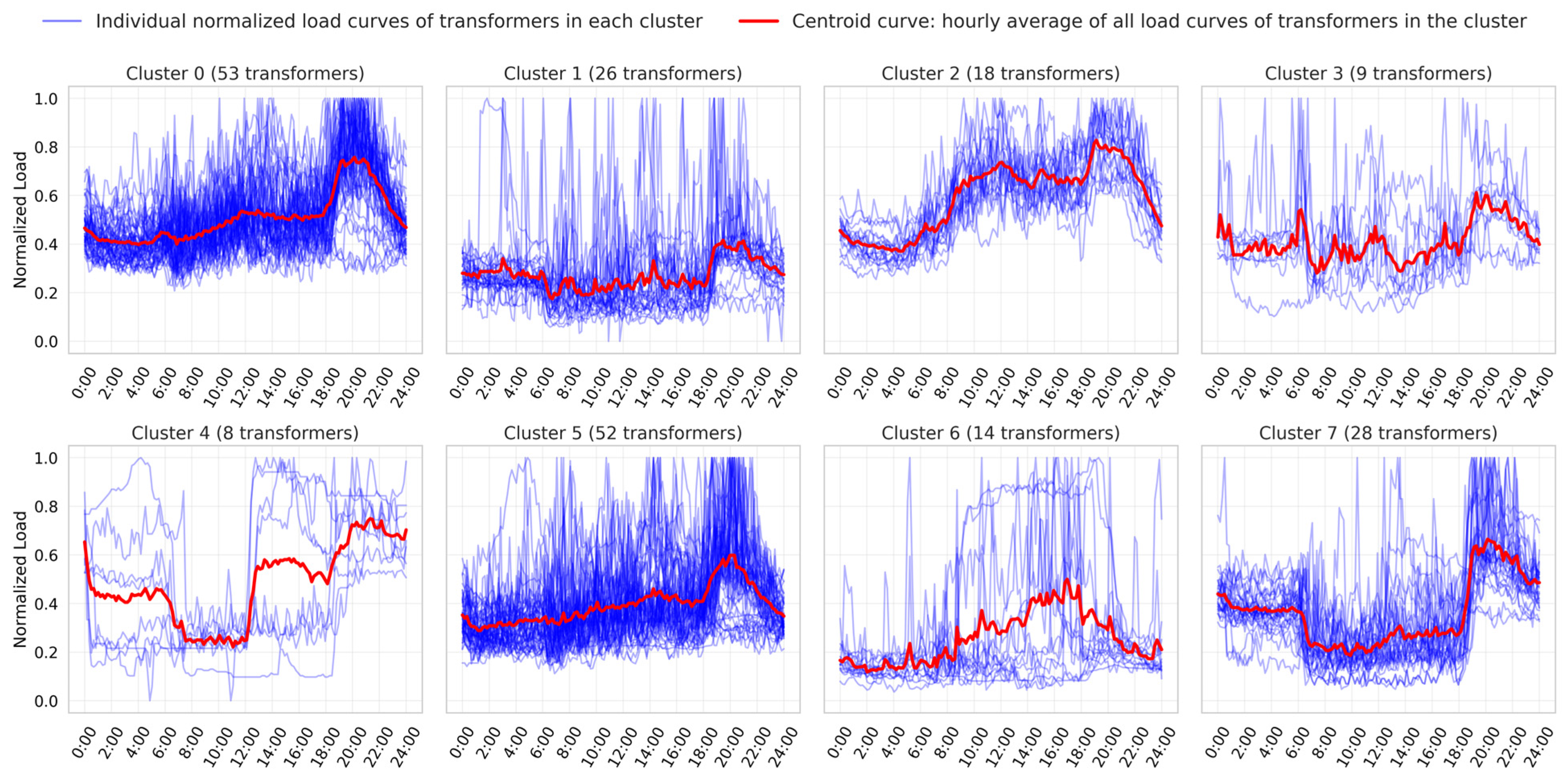
| Cluster 0 | 53 | 25.5 |
| Cluster 1 | 26 | 12.5 |
| Cluster 2 | 18 | 8.7 |
| Cluster 3 | 9 | 4.3 |
| Cluster 4 | 8 | 3.8 |
| Cluster 5 | 52 | 25.0 |
| Cluster 6 | 14 | 6.7 |
| Cluster 7 | 28 | 13.5 |
| Parameter | Description | Value |
|---|---|---|
| n_estimators | Number of trees | 10 |
| learning_rate | Learning rate | 0.1 |
| num_leaves | Maximum number of leaves per tree | 10 |
Disclaimer/Publisher’s Note: The statements, opinions and data contained in all publications are solely those of the individual author(s) and contributor(s) and not of MDPI and/or the editor(s). MDPI and/or the editor(s) disclaim responsibility for any injury to people or property resulting from any ideas, methods, instructions or products referred to in the content. |
© 2025 by the authors. Licensee MDPI, Basel, Switzerland. This article is an open access article distributed under the terms and conditions of the Creative Commons Attribution (CC BY) license (https://creativecommons.org/licenses/by/4.0/).
Share and Cite
Torres-Bermeo, P.; Varela-Aldás, J.; López-Eugenio, K.; Velasco, N.; Palacios-Navarro, G. Optimization of Electric Transformer Operation Through Load Estimation Based on the K-Means Algorithm. Energies 2025, 18, 3755. https://doi.org/10.3390/en18143755
Torres-Bermeo P, Varela-Aldás J, López-Eugenio K, Velasco N, Palacios-Navarro G. Optimization of Electric Transformer Operation Through Load Estimation Based on the K-Means Algorithm. Energies. 2025; 18(14):3755. https://doi.org/10.3390/en18143755
Chicago/Turabian StyleTorres-Bermeo, Pedro, José Varela-Aldás, Kevin López-Eugenio, Nancy Velasco, and Guillermo Palacios-Navarro. 2025. "Optimization of Electric Transformer Operation Through Load Estimation Based on the K-Means Algorithm" Energies 18, no. 14: 3755. https://doi.org/10.3390/en18143755
APA StyleTorres-Bermeo, P., Varela-Aldás, J., López-Eugenio, K., Velasco, N., & Palacios-Navarro, G. (2025). Optimization of Electric Transformer Operation Through Load Estimation Based on the K-Means Algorithm. Energies, 18(14), 3755. https://doi.org/10.3390/en18143755