Quantifying the System Benefits of Ocean Energy in the Context of Variability: A UK Example

Abstract

Recent studies have shown benefits of using tidal stream and wave energy in the electricity generation mix to improve supply–demand balancing on annual/subannual timeframes. This paper investigates this further by considering the variability of solar photovoltaic, onshore and offshore wind, wave, and tidal stream over multiple years. It also considers their ability to match with electricity demand when combined. Variability of demand and generation can have a significant impact on results. Over the sample of five years considered (2015–2019), demand varied by around 3%, and the availability of each renewable technology differed by up to 9%. This highlights the importance of considering multiple years of input data when assessing power system impacts, instead of relying on an ‘average’ year. It is also key that weather related correlations between renewable resources and with demand can be maintained in the data. Results from an economic dispatch model of Great Britain’s power system in 2030 are even more sensitive to the input data year, with costs and carbon emissions varying by up to 21% and 45%, respectively. Using wave or tidal stream as part of the future energy mix was seen to have a positive impact in all cases considered; 1 GW of wave and tidal (0.57% of total capacity) reduces annual dispatch cost by 0.2–1.3% and annual carbon emissions by 2.3–3.5%. These results lead to recommended best practises for modelling high renewable power systems, and will be of interest to modellers and policy makers.

1. Introduction

There is an ongoing need to decarbonise the global energy system, to meet net-zero targets and limit the impacts of climate change. Increased adoption of renewable energy generation is expected to contribute significantly to this [1]. The 2022 British Energy Security Strategy set a target of up to 50 GW of offshore wind by 2030 (a 36 GW increase on the existing level) and a five-fold increase in solar power from the present 14 GW is expected by 2035 [2]. It is possible that ocean energy (wave and tidal stream) can contribute towards the growth in renewable electricity generation. A significant share of the European wave and tidal resource is in the UK, estimated as 10–24.8 GW and 5.2–11.5 GW, respectively, [3,4,5]. The levelised cost of ocean energy is significantly greater than more established wind and solar technologies. However, their cost reduction trajectory could be steeper given that they are at an earlier stage of development. Whilst unlikely to ever be as cheap as wind and solar from a levelised cost of energy (LCOE) perspective, their potential to enhance system performance may result in system cost improvements that outweigh their LCOE cost premium, whilst also providing energy security benefits [6,7,8,9,10,11,12]. In this work, these potential benefits are further explored while considering the variability of electricity demand and intermittent renewable generation over differing timescales.

Whilst it is clear that expanding the deployment of energy storage and demand flexibility is critical for balancing variable renewable supply to variable demand, it comes at a cost. Research is showing that diversifying the renewable technology mix by including wave and/or tidal, the supply–demand balance can be enhanced, reducing the need for energy storage [13].

To explore this, it is important to consider the variability of both supply and demand. It is also important to capture the weather-driven links between renewable generation and demand. Renewable generation technologies are mostly intermittent, their output a function of the weather, and thus, not always available when required. Electricity demand also depends on the weather, driven largely by temperature, but wind speed and cloudiness also contribute to heating demand (e.g., [14,15,16,17]). Therefore, demand and renewable generation availability are not independent. The worst case for the UK is a calm, cold evening where wind and solar output is limited, but low temperatures push up demand [1,15]. In addition, there is also a weak negative correlation between wind speed and solar irradiance in the UK [18]. Both demand and renewable generation exhibit variability over a wide range of timescales, from almost instantaneous, through hourly, daily, weekly, seasonally, annually, and over longer timescales [19,20].

It follows that a key challenge with modelling high-renewable energy systems is to accurately capture the correlations between weather patterns and demand, whilst keeping within reasonable computational limits [21].

One approach to assess the inter-annual variability uses load duration curves (LDCs) [22]. LDCs show the power exceeded for incremental fractions of the year, sorted by demand. However, this simplification removes the temporal fluctuations and correlations between different sources. Using capacity curves to represent variable renewable energy output in energy systems models has also been identified to result in a poor representation of the hourly availability [23].

Another method to ease computational limits in energy system modelling involves the use of selected ‘time slices’ to represent example seasonal days of demand and generation over multiple years. It has been found that optimal solutions differ dramatically when converting hourly data to periods of lower resolution, with a risk of under-representing the variable nature of renewable resource and demand [24].

Finally, some existing power systems models make use of Monte Carlo simulations, to represent a number of scenarios (usually of the order of 100–1000) for intermittent renewable availability [23,25]. However, this method often involves running multiple years of historical or simulated weather data against a single demand profile, which does not correlate with the weather data.

More recent technical studies modelling high renewable future energy systems have included the use of multiple specific weather years for intermittent generation and demand [21,26], but this method is not commonplace in the scientific literature. To the authors’ knowledge, no scientific paper has been published which analyses the impact of consistent demand and generation inputs for multiple years of data on electricity dispatch modelling of the power system in Great Britain (GB).

The motivation for this work was to begin to explore the implications of variability in renewable energy resource data when modelling energy systems. Within this, the specific case of investigating the inclusion of ocean energy (wave and tidal stream) as part of a future energy mix in Great Britain was studied. This uses a series of credible scenarios, adapting those of the National Energy System Operator. Our work uses five years of consistent historical data to explore this, although the limitations of this small sample are acknowledged. Specifically, five years of annual timeseries with hourly resolution are used, for electricity demand data with the corresponding availability of five intermittent renewable resources: solar photovoltaic (PV), onshore and offshore wind, wave, and tidal stream. It is an extension of work aiming to quantify the power system benefits from ocean energy deployments [27]. Our work has the novelty of:

• Examining five years of consistent demand and generation data for the GB power system, including ocean energy, using both statistical metrics and a power system optimisation tool;
• Investigating the potential benefits of ocean energy for power system dispatch in GB for five consecutive years of data.

The rest of this paper is structured as follows. The methodology is outlined in Section 2 with the input data sources (Section 2.1), their analysis (Section 2.2), and the economic dispatch model used to assess the impact of including ocean energy (Section 2.3). Results and discussion are provided for two themes: firstly, the timeseries of demand and renewable generation availability (Section 3.1), and secondly, the outputs from the dispatch model (Section 3.2) both without and with ocean energy. This is followed by a summary of the results (Section 3.3), limitations and further work (Section 3.4), and conclusions (Section 4). This is illustrated schematically in Figure 1.

2. Methods

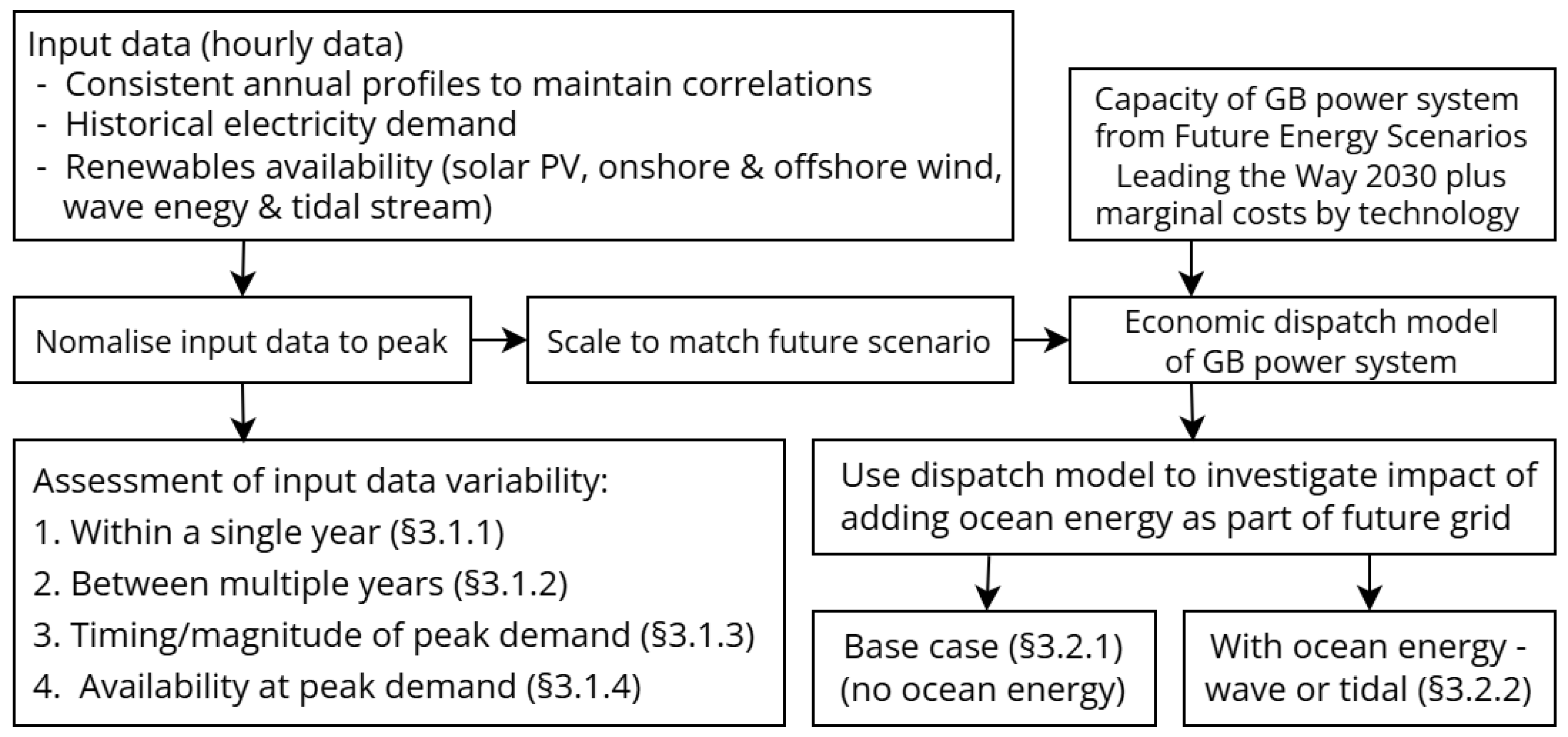
This work aims to give an illustration of the inherent variability when assessing future energy systems, specifically investigating the impact of including ocean energy as part of the future generation mix. This focuses on the inter-annual variability between years, but also examines the intra-annual variability including timing of peak demand within each year. Hourly timeseries of both electricity demand and renewable generation availability were produced and assessed for five historical years (2015–2019). These timeseries were then scaled to represent a future (2030) energy scenario in an economic dispatch model, and the variability in the results also assessed.

The methodology can be summarised as follows:

• For each of the five input years, hourly timeseries of electricity demand and renewable generation availability were derived.
• These demand and availability timeseries were analysed, considering variability within and between years, and at times of peak demand.
• An economic dispatch model scenario was developed, using these hourly timeseries as input data. Differing cases were then assessed using the model:

  (a)

  A baseline case for each of the five years;

  (b)

  Sensitivity analysis cases to explore the impact of including ocean energy in the future generation mix.

Further details on 1–3 are provided in Section 2.1, Section 2.2 and Section 2.3 below. Additional information is provided in the paper outlining the modelling framework [27].

Within this work, the five years of data between 2015 and 2019 are used, considering both the historical electricity demand and availability of intermittent renewable generation in each year. Importantly, each model run uses input data from a consistent year, thus accounting for differences in weather patterns within and between years. As 2020 and subsequent years were impacted by the COVID-19 pandemic, they are not considered in this analysis.

The electricity grid for Great Britain is considered in this work, which covers Scotland, England, and Wales. The whole island of Ireland is a separate electricity grid, although interconnected to GB by HVDC links. For the economic dispatch modelling, the GB grid was split into nine geographical zones based on National Grid boundaries to assess transmission constraints [27]. However, for simplicity, the zonal demand, availability, and model outputs were then aggregated and the GB grid considered as a whole in this analysis of variability.

The future electricity demand and assumed mix of installed generation capacity was developed to be consistent with the Future Energy Scenarios (FES) published in 2021 by the GB energy system operator (ESO), National Grid ESO [28]. For this work, the high-ambition ‘Leading the Way’ (LTW) pathway has been used, considering projections for 2030, hereafter referred to as FES LTW 2030.

2.1. Model Input Data Timeseries

The economic dispatch model (outlined in Section 2.3) requires hourly timeseries of (1) electricity demand and (2) availability for intermittent renewable generation technologies. The process of developing these timeseries is summarised below, with further details in [27].

A timeseries of GB electricity demand for each of the five years (2015–2019) was obtained from the National Grid data portal [29]. This was linearly scaled to meet the projected increase in both total and peak demand in FES LTW 2030, in GWh/yr and GW, respectively. The total and peak demand, thus, maintain their historical variability, both hour-by-hour and between years. It is expected that the future demand profile, especially at the hourly level, will change significantly from today, with the electrification of industry, heating, and transportation, and also with the emergence of load shifting and grid balancing services (e.g., [30,31]). Detailed consideration of demand flexibility or energy storage was not within the scope of the study. A previous study of the Isle of Wight, UK, found that when comparing a typical demand profile with a flat demand profile over the whole year, there were similar levels of supply demand enhancement when tidal was added to the mix [6].

Hourly timeseries were created for each of the five years (2015–2019) with the availability for five intermittent renewable generation sources: solar PV, onshore and offshore wind, wave, and tidal stream. Multiple locations were used for each technology to represent the geographical spread of the resource, and allocated to the nine model zones based on National Grid ESO FES [28]. Details of the sites used and zonal allocation process are given in [27]. The overall availability for each technology was then aggregated at a GB level for this analysis of variability.

The availability timeseries for solar PV, onshore and offshore wind were all generated using the Renewables.ninja tool [32]. This software takes solar irradiance and wind speed data from NASA’s MERRA reanalysis [33] and applies a Virtual Wind Farm model [34] and a Global Solar Energy Estimator model [35], respectively, to generate hourly timeseries of wind and solar generation availability at the specified coordinates.

The timeseries for wave energy were developed from hourly hindcast data using a 2030 target power matrix for the CorPower Ocean WEC. The hindcast were from Copernicus Marine Service Information, specifically the Arctic Ocean Wave Hindcast [36] and the Atlantic -Iberian Biscay Irish- Ocean Wave Reanalysis [37]. The PacIOOS WaveWatch III model [38] was used to identify areas of interest, but because of its coarse spatial resolution, the more precise Copernicus models were used for individual sites.

Tidal stream availability timeseries were created for specific GB sites with good resource based on previous modelling using the Thetis coastal ocean model [9]. This assumed an average annual capacity factor of 40% for tidal stream turbines.

The installed capacity of wind and solar in all model scenarios is significantly greater than for ocean energy, as shown in Table 1. Additionally, a larger number of sites were considered for these technologies, which will lead to some averaging over the UK, leading to lower variability.

One of the five years considered was a leap year, namely 2016, adding an extra 24 h of data to that year. When considering summated metrics, such as total dispatch cost, the extra day introduces a small discrepancy, although at <0.3% this is not significant compared to the inter-annual variability observed.

Table 1. Installed capacities (GW) for intermittent renewable generation technologies for baseline, plus wave and tidal sensitivities. Total renewable generation (MWh) was kept consistent between sensitivities.

	Installed Capacity (GW)			Capacity
Technology	Baseline	Wave Sensitivity	Tidal Sensitivity	Factor
Solar PV	39.70	39.70	39.70	0.130
Onshore wind	26.33	26.33	26.33	0.289
Offshore wind	47.33	47.33–35.63	47.33–38.08	0.439
Wave	0	0–10	0	0.513
Tidal stream	0	0	0–10	0.406

Table 1. Installed capacities (GW) for intermittent renewable generation technologies for baseline, plus wave and tidal sensitivities. Total renewable generation (MWh) was kept consistent between sensitivities.

	Installed Capacity (GW)			Capacity
Technology	Baseline	Wave Sensitivity	Tidal Sensitivity	Factor
Solar PV	39.70	39.70	39.70	0.130
Onshore wind	26.33	26.33	26.33	0.289
Offshore wind	47.33	47.33–35.63	47.33–38.08	0.439
Wave	0	0–10	0	0.513
Tidal stream	0	0	0–10	0.406

2.2. Demand and Renewable Generation Availability Analysis

Once the future timeseries of hourly demand and availability of intermittent renewable generation were developed, preliminary analysis was undertaken to explore the annual and inter-annual variability of these inputs. To facilitate comparison, the availability data was normalised by the peak for each year. This preliminary analysis reviewed both the whole year and also focused on times of peak demand. To assess the availability at times of peak demand, the hours of each year were sorted by demand (high to low). The corresponding renewable generation availability was then calculated for the top $X\%$ hours of the year, where $X\in 0.5,1,2,5,10,25,50,75,100$.

2.3. Economic Dispatch Modelling to Consider the Impact of Including Ocean Energy

Economic dispatch modelling has been utilised as a tool here to quantify the ability for different renewable technology mixes to meet demand. The hourly generation and demand timeseries described in Section 2.1 are used as inputs for an optimisation function that is set to match demand with supply for every hour of the year with the objective of minimising annual cost. The linear optimal power flow function is used in the Python for Power Systems Analysis (PyPSA) software package, v0.19.1 [39] (Python 3.9.7) to perform this optimisation. Each PyPSA model run takes minutes on a modern laptop when using the Gurobi solver, v9.5.1. However, it is noted that significant additional computing resource is required to derive the renewable availability input data used in the analysis.

The future mix of electricity generation capacity and capability was created to be consistent with FES LTW 2030. In the wave and tidal sensitivities, some of the predicted growth in offshore wind capacity was instead allocated to ocean energy, either wave or tidal stream. An increasing proportion of ocean energy was considered, keeping the total energy generation (MWh) constant when doing so, to give a fair comparison. The differing capacity factor (CF) assumptions for offshore wind, wave, and tidal stream mean that the total installed capacity therefore varies with the technology mix, but the total renewable energy generation available remains constant. Installed capacities for intermittent renewable sources are given in Table 1.

The marginal generation cost was taken as the fuel cost (including carbon costs for fossil fuels and waste costs for nuclear) based on [40]. The marginal cost for variable renewables were assumed to be zero. Therefore, the economies of building and operating the generation is not directly modelled. The model does include storage, in the form of batteries and pumped hydro, plus interconnectors to neighbouring counties, and a simplified representation of demand-side response. All of these have installed capacities in line with FES LTW 2030, which account for significant electrification of the energy system. Further details are given in [27].

These inputs were then run through the economic dispatch model described in [27] and the variation in output metrics was reviewed. All other inputs were kept constant with the baseline from [27], which also explored the sensitivity of technologies used and grid constraints, and describes the model validation.

The inter-annual variation of the output metrics from the dispatch model for the 5 years of input data were reviewed for the different cases: (a) baseline case without any ocean energy and (b) sensitivity analysis cases investigating including some wave or tidal energy as part of the electricity generation mix. Eight metrics have been used to quantify the impact, with paired Student’s t-test used to assess significance.

3. Results and Discussion

Results are first presented from the analysis of the hourly timeseries of electricity demand and intermittent renewable availability. This covers the variability over both a single year and then between years, to illustrate the variation in the input data used. The timing and magnitude of peak demand is reviewed, along with the availability of intermittent renewable generation at peak times, showing how these both vary between years.

Following this, outputs from the economic dispatch modelling quantify the system benefits of ocean energy and illustrate sensitivity to the year of input data used. Both a baseline case without ocean energy and examples including an increasing proportion of ocean energy as part of the future generation mix are presented.

A summary of the results and their implications is then given in Section 3.3, followed by a brief discussion on limitations.

3.1. Timeseries of Demand and Availability

3.1.1. Variability over Single Year

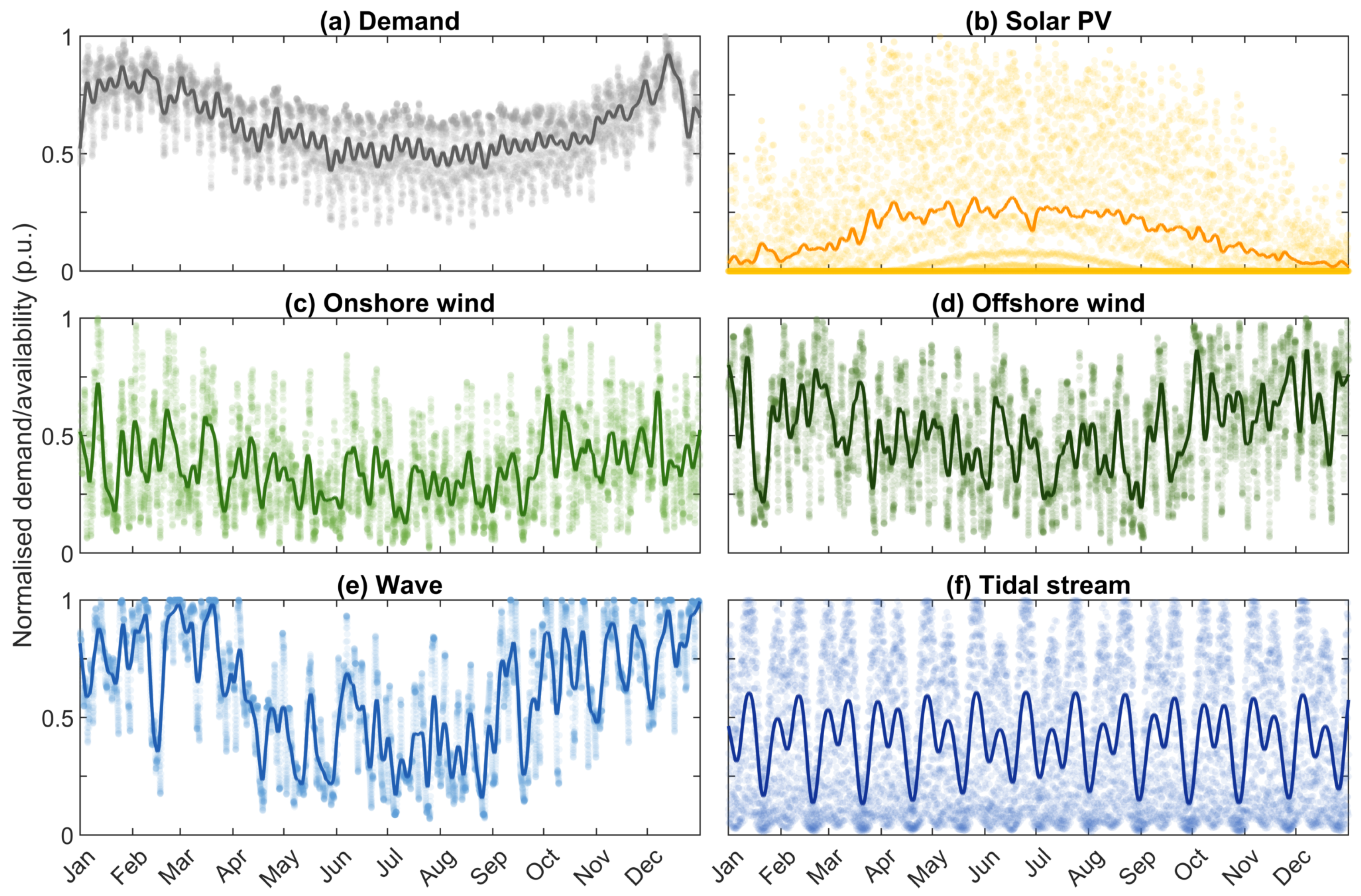
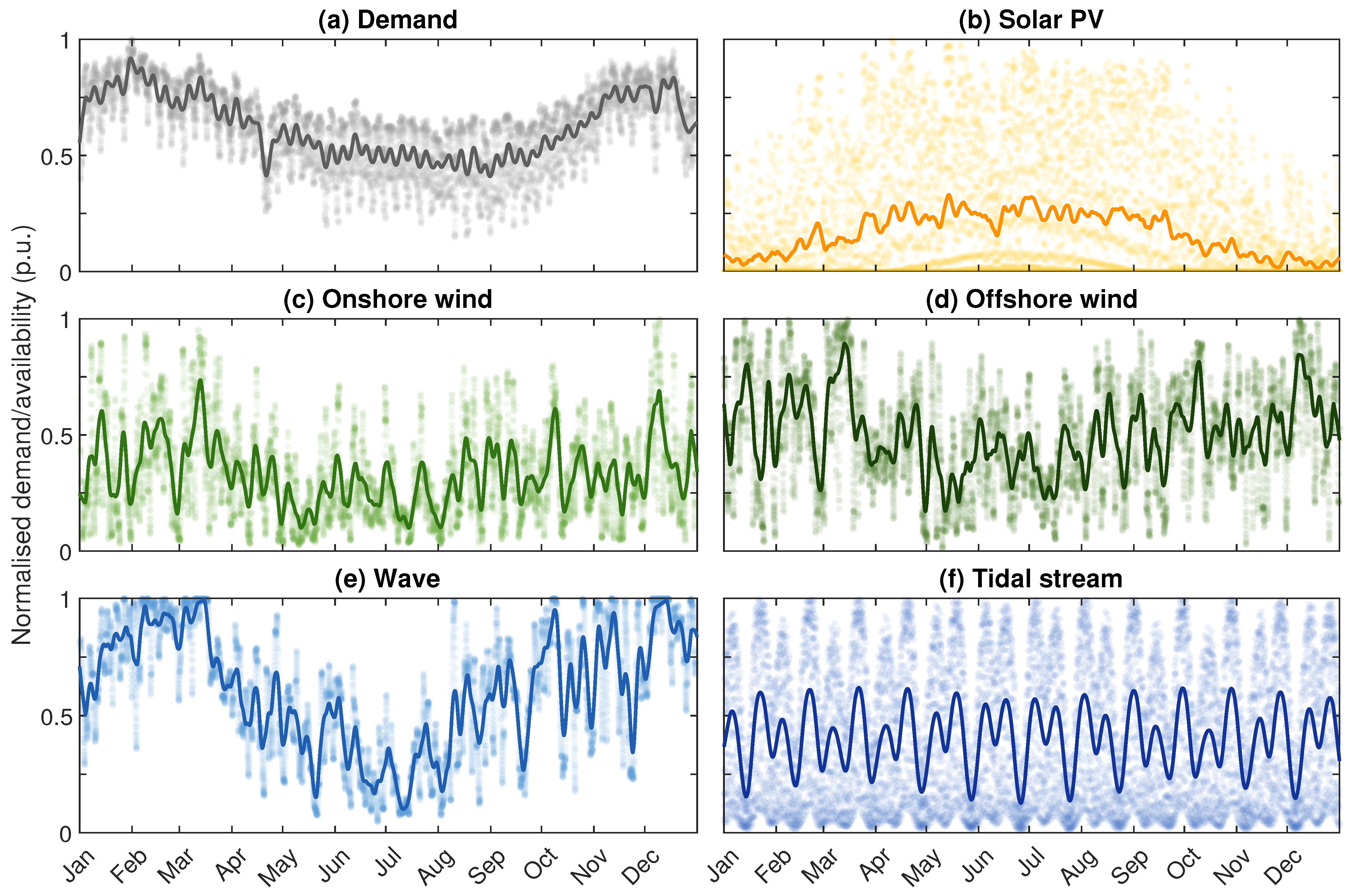
The variability of electricity demand and the corresponding availability of intermittent renewable generation over a single year is first discussed, using 2019 as an example average year. Summary statistics are shown in

Table 2. Mean, median, minimum, and standard deviation of normalised hourly electricity demand and renewable generation availability for 2019.

	Demand	Solar PV	Onshore Wind	Offshore Wind	Wave	Tidal Stream
Mean	0.624	0.166	0.332	0.500	0.606	0.406
Median	0.631	0.001	0.299	0.496	0.627	0.355
Minimum	0.152	0.000	0.031	0.019	0.047	0.010
Std.	0.163	0.252	0.195	0.226	0.271	0.292

. Mean annual electricity demand is approximately 62% of the hourly peak demand, with minimum demand around 15% of peak. Unsurprisingly, the median availability for solar PV is virtually zero, as it is dark approximately half the hours of the year, with no solar output. The resource availability of the other renewable technologies never quite drops to zero on an hourly timescale across the GB grid. The mean availability relates to the capacity factor assumptions used in the modelling, which varies by technology. Offshore wind has a higher availability than onshore wind (50% versus 33%), while ocean energy could theoretically have an availability of around 60% for wave and 40% for tidal stream, although this is still to be commercially demonstrated.

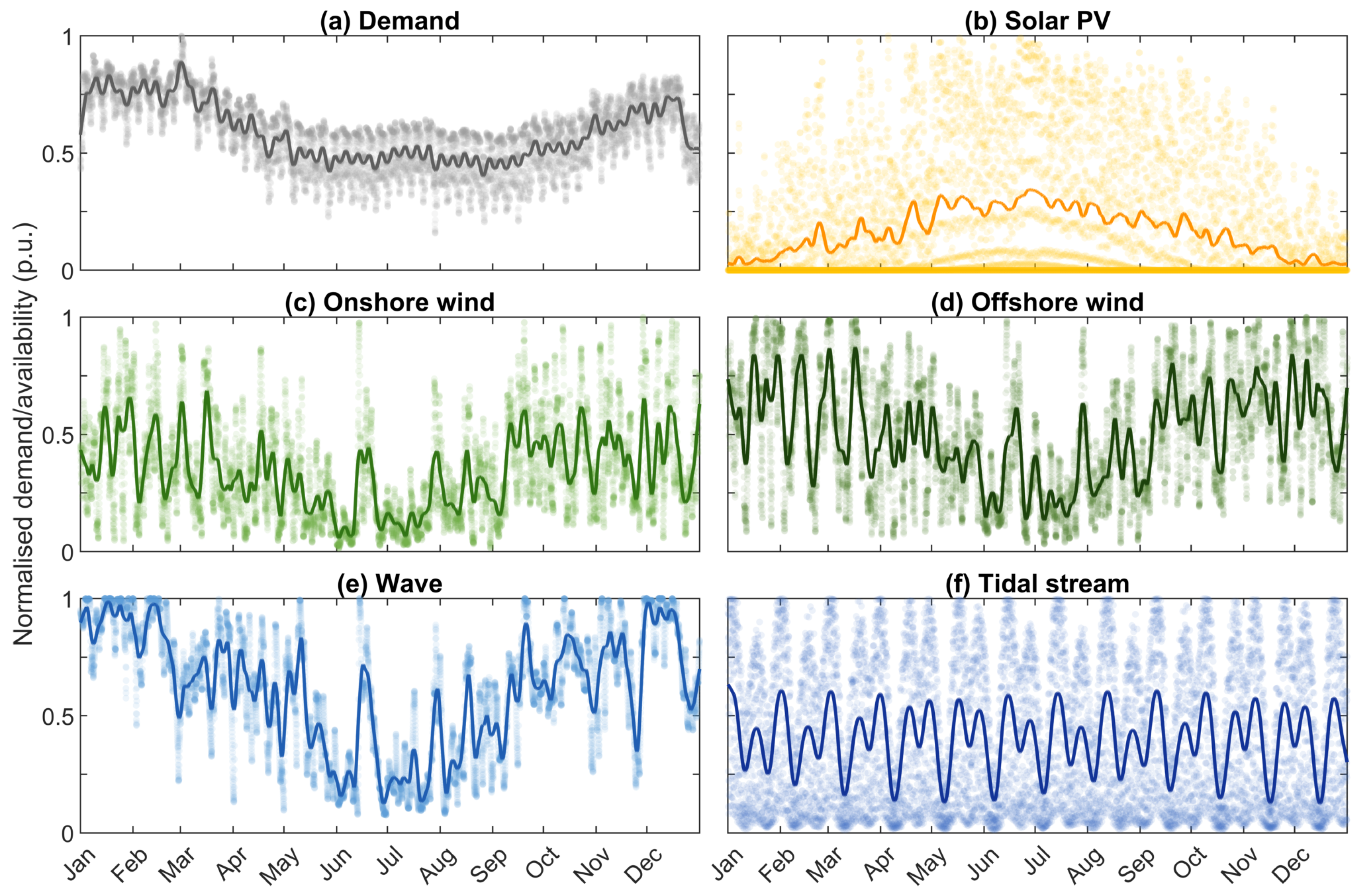
This variability over the year is shown graphically in Figure 2, highlighting the clear seasonal trend in the demand—higher over the winter months. There is also a clear reduction in demand at weekends and holiday periods, particularly Easter (21 April 2019) and around Christmas/New Year. This trend was observed across Europe in [14]. Comparable figures for 2015–2018 are shown in Appendix A, Figure A1, Figure A2, Figure A3 and Figure A4. Availability statistics for 2015–2019 are tabulated in

Table A1. Mean normalised hourly availability for each renewable technology and year of input data.

Year	Solar PV	Offshore Wind	Onshore Wind	Wave	Tidal Stream
2015	0.165	0.380	0.533	0.643	0.409
2016	0.163	0.323	0.488	0.588	0.404
2017	0.164	0.363	0.522	0.601	0.402
2018	0.168	0.343	0.499	0.609	0.399
2019	0.166	0.332	0.500	0.606	0.406
Mean	0.165	0.348	0.508	0.610	0.404

,

Table A2. Median normalised hourly availability for each renewable technology and year of input data.

Year	Solar PV	Offshore Wind	Onshore Wind	Wave	Tidal Stream
2015	0.002	0.328	0.526	0.647	0.346
2016	0.002	0.274	0.466	0.596	0.333
2017	0.002	0.330	0.519	0.615	0.333
2018	0.002	0.302	0.489	0.640	0.331
2019	0.001	0.299	0.496	0.627	0.355
Mean	0.002	0.306	0.499	0.625	0.340

,

Table A3. Minimum normalised hourly availability for each renewable technology and year of input data.

Year	Solar PV	Offshore Wind	Onshore Wind	Wave	Tidal Stream
2015	0.000	0.020	0.040	0.074	0.012
2016	0.000	0.017	0.046	0.048	0.011
2017	0.000	0.019	0.043	0.069	0.012
2018	0.000	0.014	0.032	0.076	0.012
2019	0.000	0.031	0.019	0.047	0.010
Mean	0.000	0.020	0.036	0.063	0.011

,

Table A4. Standard deviation of hourly normalised availability for each renewable technology and year of input data.

Year	Solar PV	Offshore Wind	Onshore Wind	Wave	Tidal Stream
2015	0.250	0.235	0.254	0.277	0.298
2016	0.244	0.208	0.236	0.280	0.298
2017	0.248	0.194	0.231	0.265	0.298
2018	0.256	0.215	0.250	0.268	0.297
2019	0.252	0.195	0.226	0.271	0.293
Mean	0.250	0.209	0.239	0.272	0.296

and

Table A5. Interquartile range of hourly normalised availability for each renewable technology and year of input data.

Year	Solar PV	Offshore Wind	Onshore Wind	Wave	Tidal Stream
2015	0.269	0.356	0.418	0.512	0.546
2016	0.278	0.272	0.371	0.491	0.546
2017	0.276	0.281	0.374	0.446	0.545
2018	0.275	0.308	0.408	0.450	0.541
2019	0.277	0.266	0.353	0.470	0.527
Mean	0.275	0.297	0.385	0.474	0.541

.

As with demand, there are clear seasonal trends in the availability of solar PV and wave, and to a lesser extent offshore and onshore wind. Conversely, the tidal stream resource is consistent over the year, albeit with daily tides and the monthly spring–neap cycle. The renewable resources all exhibit variability over multiple timescales, and periods of resource offsetting are observable between these technologies at both hourly and seasonal resolutions, as has been observed in other studies (e.g., [6,9,42,43,44]).

3.1.2. Inter-Annual Variability

Having looked at variation within an individual year, the variability between different years can then be explored. The total, mean, and peak GB electricity demand for 2015–2020 is shown in

Table 3. Total, mean, peak, and minimum GB electricity demand for 2015–2020, and FES LTW 2030 projection (with percentage difference to 2015–2019 mean).

Year	Total (TWh)	Mean (GW)		Peak (GW)
2015	323.3	36.90	(+3.6%)	55.65	(+3.4%)
2016	314.3	35.78	(+0.4%)	53.70	(−0.2%)
2017	307.2	35.07	(−1.6%)	52.25	(−2.9%)
2018	310.7	35.47	(−0.4%)	55.78	(+3.7%)
2019	305.8	34.90	(−2.0%)	51.67	(−4.0%)
2020 *	286.7	32.63	(−8.4%)	52.40	(−2.6%)
⋮
2030	417.9	47.67	(+33.8%)	67.3	(+25.1%)

* 2020 not considered further in the analysis due to COVID-19.

. The considerable reduction in total/mean demand in 2020 due to the COVID-19 pandemic is clear, so data from 2020 onwards was not considered further in the analysis.

The total and mean demand are linked and generally reduce year-on-year, following the trend over the past decade for GB electricity demand falling as a result of energy efficiency improvements [45]. However, peak demand does not follow this pattern, as it is predominantly due to specific weather conditions. Total electricity demand is forecast to increase significantly over the coming decades with further electrification of heating and transport [28]. The National Grid ESO projections for the FES LTW 2030 scenario are also shown in Table 3.

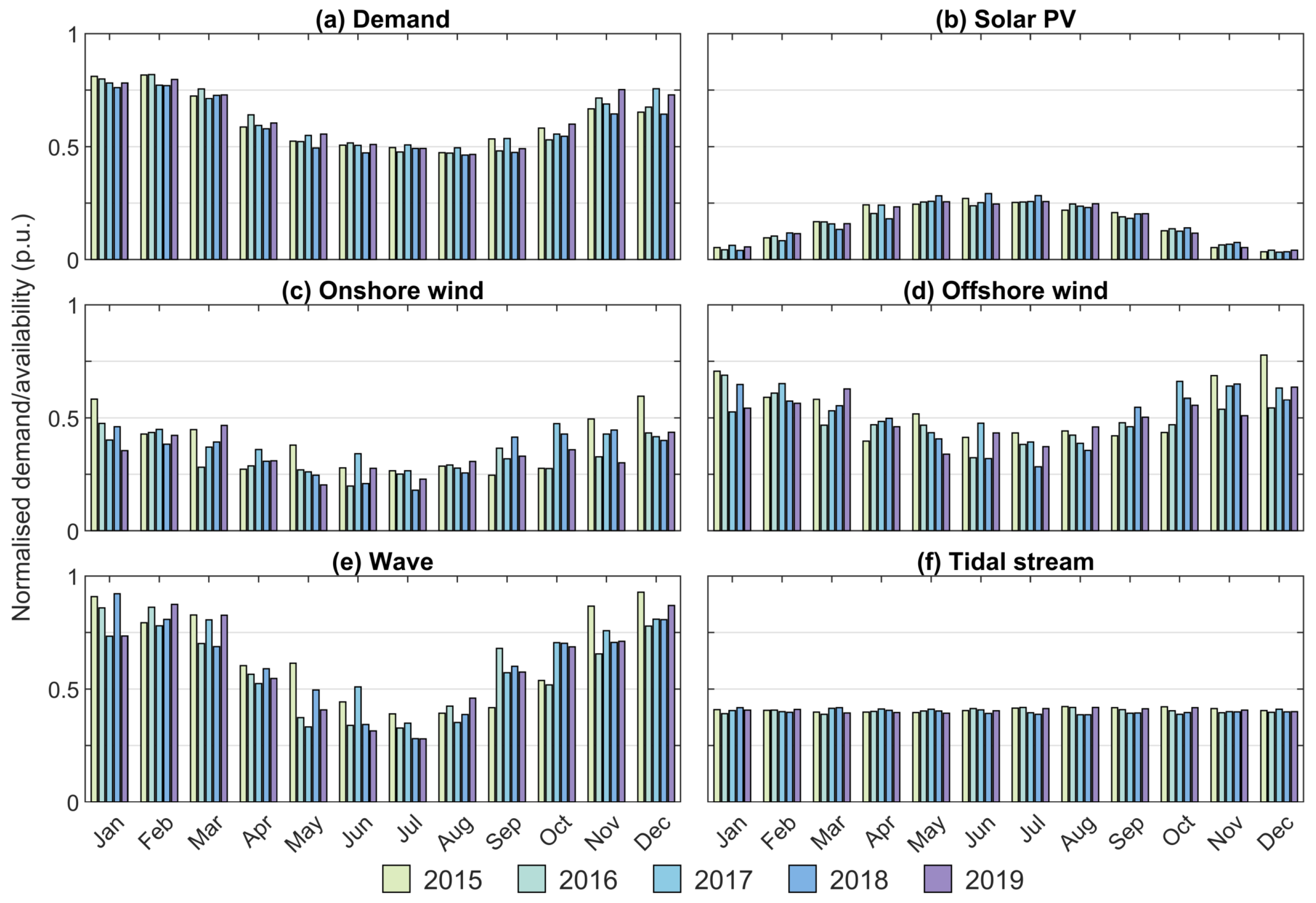
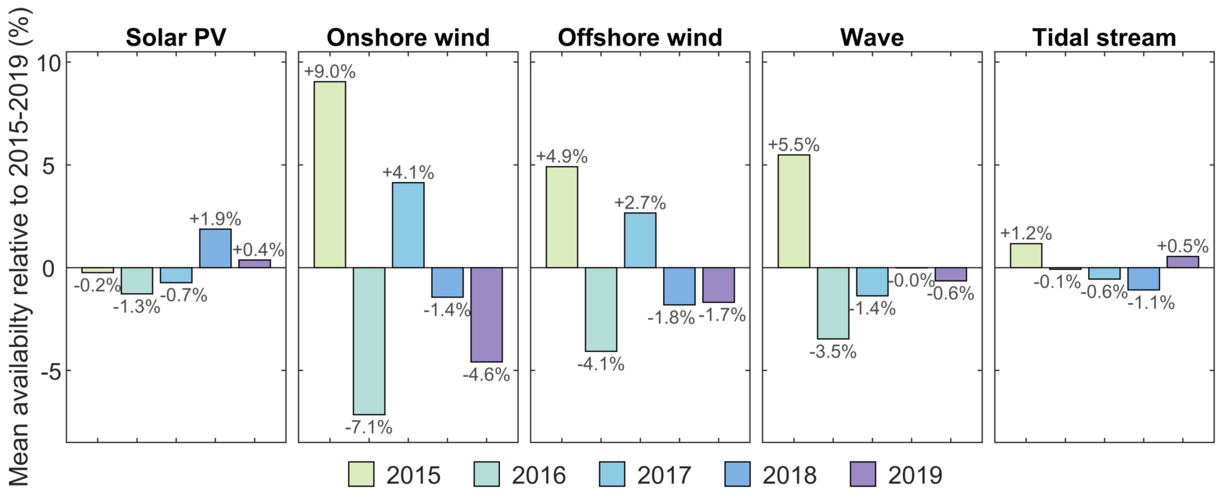
The corresponding annual variation in availability for the intermittent renewable generation technologies is shown for 2015–2019 in Figure 3, relative to the mean of that period. We determined that 2015 was a higher wind year while 2016 was lower-than-average, which is apparent in the mean availability of both onshore and offshore wind and of wave; this is more pronounced in onshore wind at +9% and −7% for 2015 and 2016, respectively. Mean availability of solar PV is relatively consistent between years of data, deviating by less than ±2% from average. The tidal resource is even less sensitive, with a variation of only ±1.2% depending on the year of input data; however, it is important to note that each year of input data is normalised, so longer-term fluctuations in the tides, such as the 18.6 year lunar nodal cycle, are excluded.

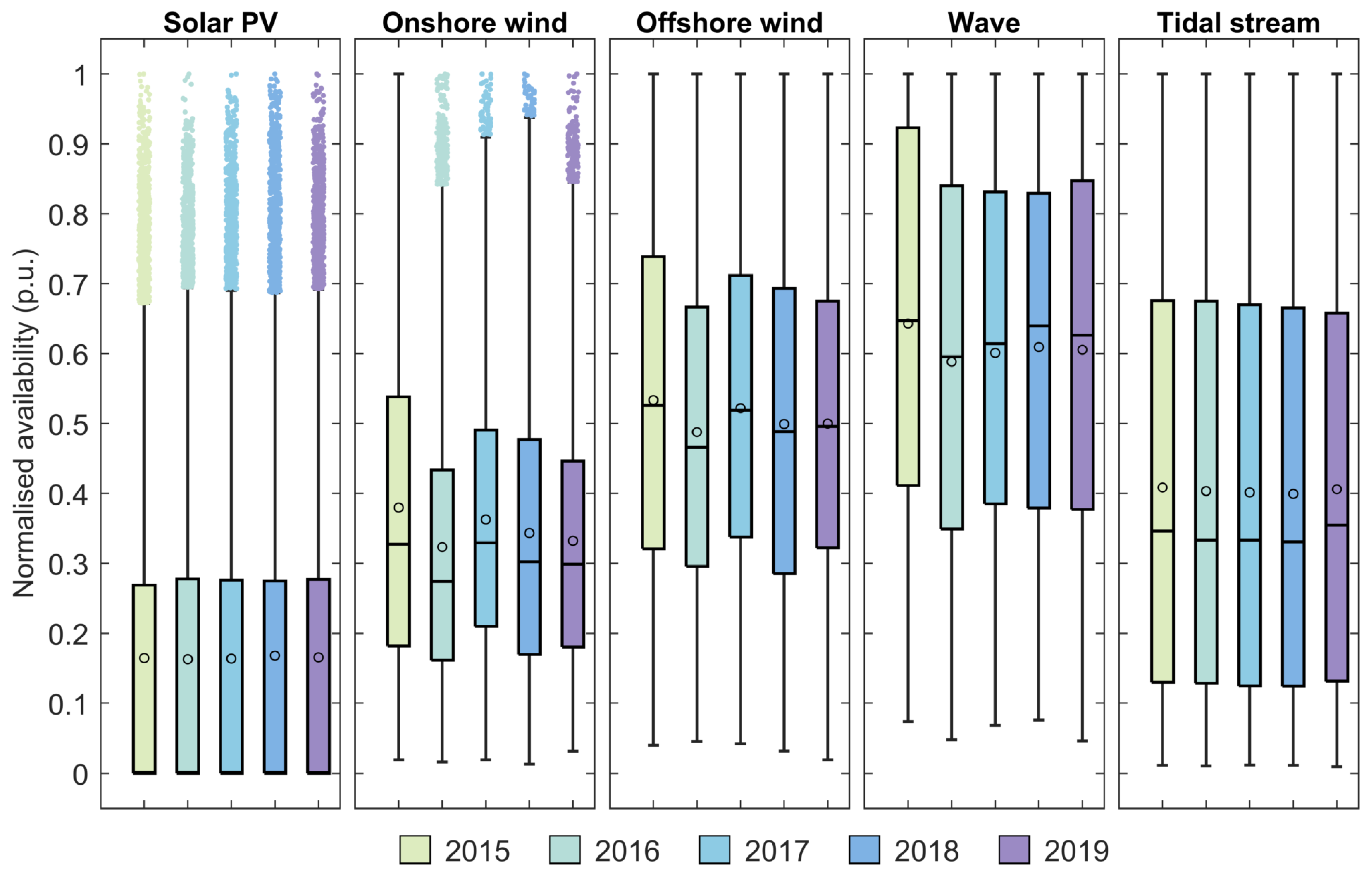
To explore this variability in more detail, the normalised distributions of demand and availability data for each technology and year are shown as box and whisker plots in Figure 4. Again, it can be seen that the solar PV and tidal-stream resource is reasonably consistent between years of input data, with mean availability of approximately 16.5% and 40%, respectively. These technologies also show a consistent interquartile range (IQR) between the years studied. There is also a greater difference between mean and median for solar (and to a lesser extend tidal) than the other renewables. This is due to the larger variance, with availability dropping to zero (or nearly in the case of tidal) every day. Tidal stream has the highest variability within the year, shown by the larger IQR, due to the semi-diurnal nature of the tides around GB. Wave energy has the highest availability, but has slightly greater variability than wind (shown by the larger IQR); however, the wave availability rarely drops as low as wind availability. This work only considers one wave energy technology. With a portfolio of different technologies, each performing differently on different regions of the sea state distribution, lower variability of wave availability might be expected, probably also with a lower mean output. The higher wind years of 2015 and 2017 are also apparent in Figure 4 when considering mean, median, and IQR, although only 2015 was higher in terms of wave resource. Key statistics describing this data are tabulated in Appendix A Table A1, Table A2, Table A3, Table A4 and Table A5, along with the monthly average demand and availability for each year of input data in Figure A5.

3.1.3. Timing/Magnitude of Peak Demand

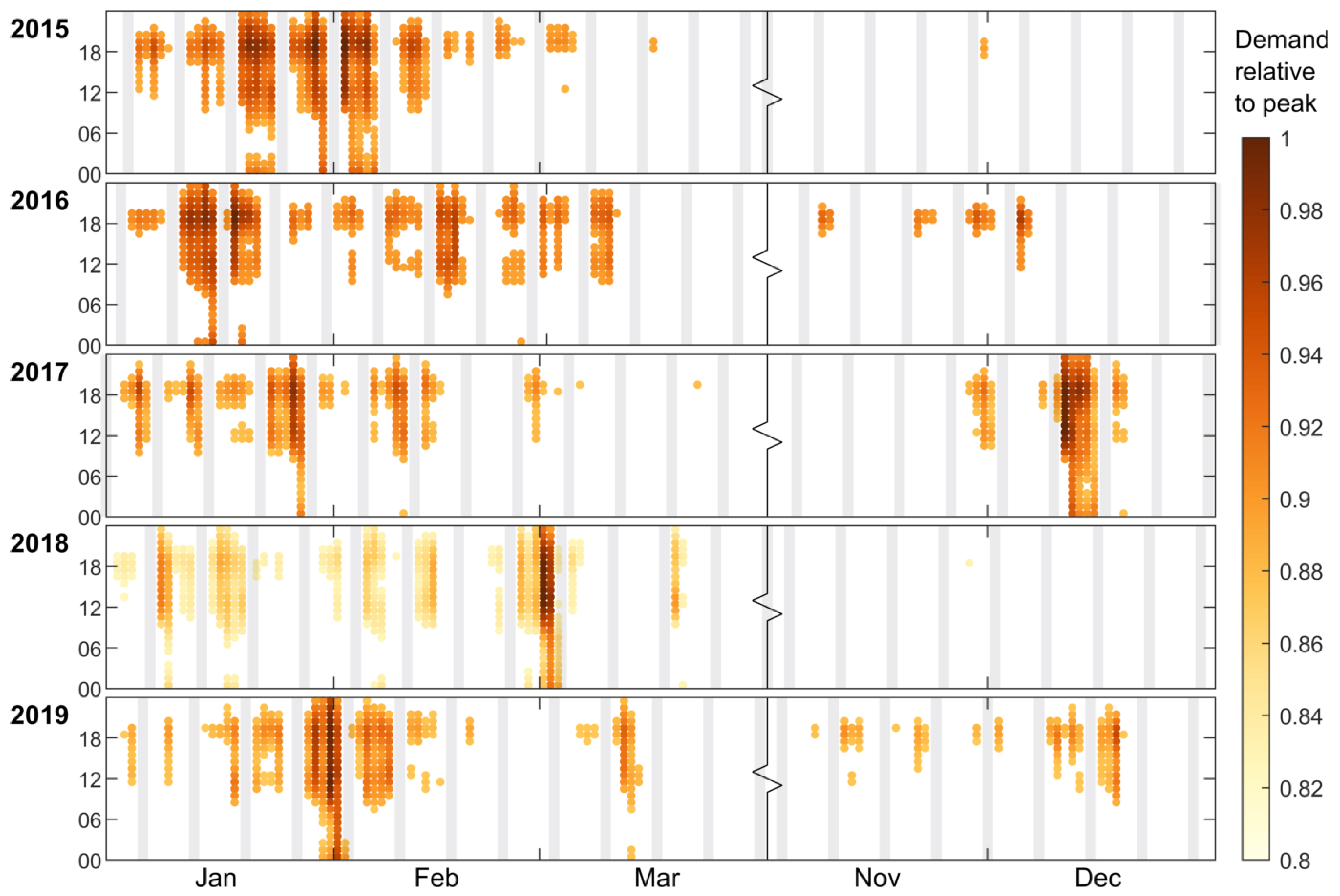
Focusing in on just the hours of peak demand, we consider just the 5% of hours with the highest demand over that year (438 h in total, ranked by demand); these are shown as a heatmap in Figure 5 for the years 2015–2019. Note that only the winter months (January–March and November–December) are shown for each year, as these contain the peak hours. This clearly shows the weekly and daily patterns of demand in GB, where there is lower demand at the weekends (shown by grey bars that rarely include the peak hours) and higher demand during the day, generally peaking around 18:00. The timing and magnitude of peak demand varies by year, although it is typically on a winter evening.

Table 4. Details of peak electricity demand for 2015–2019.

Year	Date and Time of Peak Demand	Fraction of Peak Demand Exceeded for:		№ hours ≥ 90% of Peak Demand
		Top 1% (88 h)	Top 5% (438 h)
2015	Monday 2–February 19:00	0.946	0.885	329
2016	Monday 18–January 18:00	0.940	0.894	364
2017	Monday 11–December 18:00	0.929	0.874	230
2018	Thursday 1–March 13:00	0.883	0.826	50
2019	Thursday 31–January 18:00	0.920	0.870	178

shows the date and hour of the peak demand, the fraction of demand exceeded for the top 1% and 5% of hours, plus the number of hours where there is ≥90% of the peak demand in that year. The date of peak demand can vary significantly, by several months, as it is related to weather patterns throughout the winter.

The peak demand for 2018 was impacted by the “Beast from the East” weather event at the end of February into early March, when significant snow fell across the UK and temperatures were around 10 °C below average [46]. This storm is clear in Figure 5. The peak in demand was also more pronounced than other years, as shown by the fact there are fewer hours of the year with ≥90% of the peak demand and a lower fraction of peak demand was exceeded by the top 1% of hours, see Table 4.

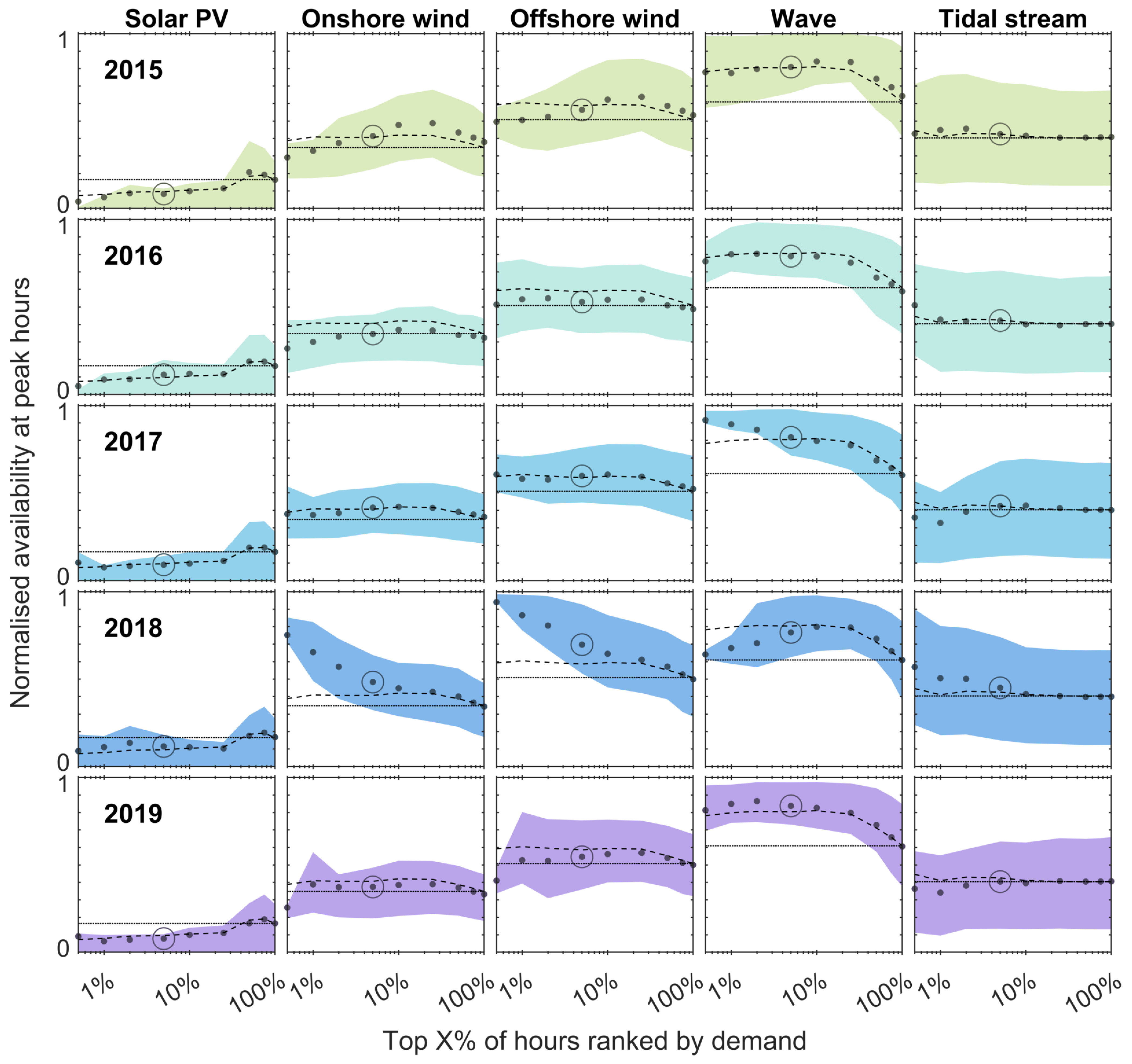
3.1.4. Availability of Renewables at Peak Demand

Due to their stochastic nature, intermittent renewable generation may or may not be available at times of peak demand in a given year. To explore this, the mean and range of availability was calculated for the top $X\%$ of hours of the year ranked by peak demand. This is shown in Figure 6, with the final point (100%) corresponding to the whole year, equivalent to Figure 4. The availability of renewables during the top 5% of demand hours is tabulated in

Table 5. Availability of renewables over top 5% of demand hours (demand shown in Figure 5).

Year	Solar PV	Onshore Wind	Offshore Wind	Wave	Tidal Stream
2015	0.083	0.414	0.564	0.809	0.426
2016	0.113	0.345	0.528	0.790	0.422
2017	0.091	0.416	0.597	0.817	0.425
2018	0.115	0.483	0.697	0.767	0.450
2019	0.079	0.374	0.547	0.838	0.404
Mean	0.096	0.406	0.586	0.804	0.426

.

Unsurprisingly, solar has a low availability over the top 25% of peak demand hours, as these tend to be on winter evenings. This is illustrated in Figure 6 by the dashed line (five-year mean availability over top $X\%$ peak demand hours) being below the dotted line (mean availability over the full period) for the top 25% of peak demand hours. Conversely, wind and wave have higher availability in the winter, and thus, the availability over the top 25% of demand hours is higher than at 100% (over the whole year). As with Figure 4, there appears to be a correlation in onshore and offshore wind availability between years, with higher availability for offshore wind. Given that tides are predictable, but decoupled from electricity demand, the mean availability of tidal stream does not vary much with demand. However, the semi-diurnal variation in tides results in a wider spread of availability at all fractions of peak demand, as illustrated by the larger IQR.

Much of the peak demand in the 2018 data happened at times with high wind resource, especially offshore. This is apparent in Figure 6, where both onshore and offshore wind show high availability at peak demand hours; even more so than the average for the five-year period, with the points and shaded IQR for that year above the dashed line. The wave resource is well correlated with demand in GB, with above average availability at all fractions of peak demand hours, especially the top 0.5–5% in 2017. However, in 2018, wave availability was only average over the top 0.5% of demand hours. The times of peak demand in the 2018 data happened to correspond better to tidal availability, but less so in 2017 and 2019.

3.2. Outputs from Dispatch Model

Having examined the variability of electricity demand and renewable generation availability, what does this mean for power systems? This section explores the outputs from the economic dispatch model (Section 2.3), showing the variation between the five different years of input data used. The model scenario is consistent with FES LTW 2030, with no ocean energy in the 2030 baseline case. Inclusion of ocean energy is explored in Section 3.2.2.

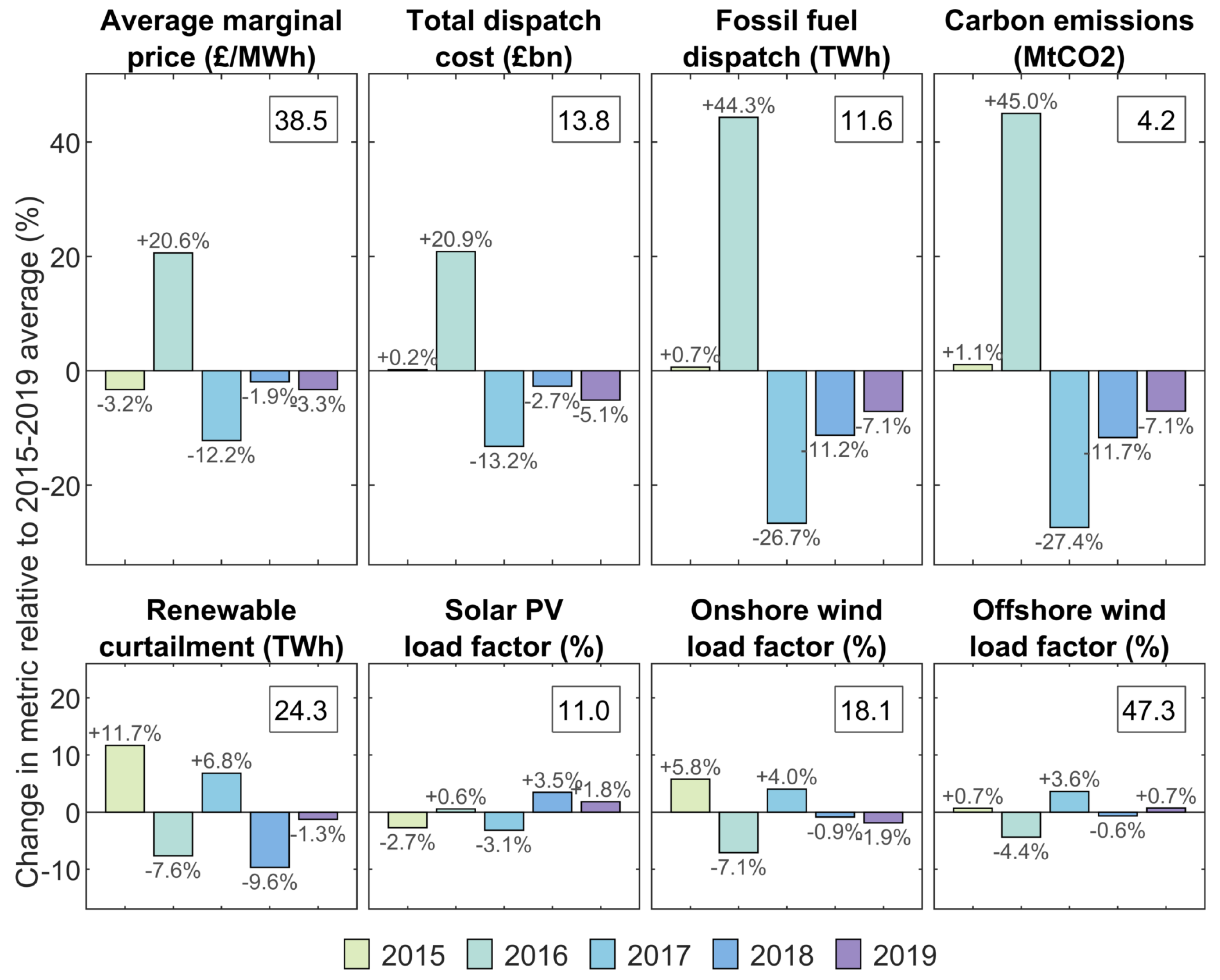
3.2.1. 2030 Baseline Case

To illustrate the potential variation in the economic dispatch results depending on the input year of data considered, a range of metrics are used. This is shown for each metric as the percentage deviation from the mean of this five-year period. Metric values for each year of input data are tabulated in Appendix A,

Table A6. Economic dispatch model metrics for base case (no ocean energy) for each year of input data.

Year	Average Market Price (GBP/MWh)	Total Dispatch Cost (Billion GBP)	Fossil Fuel Dispatch (TWh)	Carbon Emissions (MtCO2)	Renewable Curtailment (TWh)	Solar PV Load Factor (%)	Onshore Wind Load Factor (%)	Offshore Wind Load Factor (%)
2015	37.2	13.8	11.7	4.27	27.1	10.8	19.2	47.6
2016	46.4	16.7	16.8	6.13	22.4	11.1	16.8	45.2
2017	33.8	12.0	8.5	3.07	25.9	10.7	18.9	49.0
2018	37.8	13.4	10.3	3.74	21.9	11.4	18.0	47.0
2019	37.2	13.1	10.8	3.93	24.0	11.3	17.8	47.6
Mean	38.5	13.8	11.6	4.23	24.3	11.0	18.1	47.3

.

The marginal price, or price to produce an additional MWh of electricity, is calculated for every hourly timestep of the dispatch optimisation. The average marginal price over the year of dispatch can, thus, be used as a proxy for the supply/demand balance in a competitive electricity market, since it is higher when system margins are tighter. Over the five-year period, the mean was 38.49 GBP/MWh, with a maximum of 46.43 GBP/MWh (+21% above the mean of the period) and minimum of 33.80 GBP/MWh (−12%). Related to this is the total dispatch cost over the year of 13.8 billion GBP ($\begin{array}{c}+21\\ -13\end{array}\%$), the total fossil fuel dispatch at 11.6 TWh ($\begin{array}{c}+44\\ -27\end{array}\%$), and the annual carbon emissions of 4.23 MtCO₂ ($\begin{array}{c}+45\\ -27\end{array}\%$). It should be noted that the total cost of dispatch is calculated as the sum-product of marginal price (in GBP/MWh) and electricity dispatch (in MWh) for every hour of the year.

At times, the intermittent renewable generation can be greater than demand, and thus, needs to be curtailed if there is insufficient storage, demand-side response, or inter-connector availability. The mean annual curtailment is 24.3 TWh ($\begin{array}{c}+12\\ -10\end{array}\%$). Finally, the mean load factors and range of variability for solar, onshore wind, and offshore wind are $11.0\begin{array}{c}+3.5\\ -2.7\end{array}\%$, $18.1\begin{array}{c}+5.8\\ -7.1\end{array}\%$, and $47.3\begin{array}{c}+3.6\\ -4.4\end{array}\%$, respectively; these refer to the amount of renewable generation actually dispatched, i.e., available at times of demand. This obviously depends on the hourly fluctuations in demand and renewable availability in each of the five years of input data.

These metrics are plotted in Figure 7 as the deviation from the five-year mean. The link between the first four metrics is clear, with higher costs and emissions in 2016 due to the greater fossil fuel dispatch that year. This is linked to the lower-than-average renewable generation in that year (see Figure 3), also visible in the below-average load factors for both onshore and offshore wind in Figure 7. The variation in carbon emissions is very closely linked to the fossil fuel dispatch, with greatest sensitivity ($\begin{array}{c}+45\\ -27\end{array}\%$) to the year of input data in the model output. Average marginal price and total dispatch cost are not quite as closely linked and show lower sensitivity ($\begin{array}{c}+21\\ -13\end{array}\%$) to the year of input data. These pairs of metrics exhibit differing response to the year of input data, highlighted by the ordering of 2018 and 2019. In these, 2019 has a greater change in costs, but conversely, 2018 has the larger change in fossil fuel dispatch and emissions.

Renewable curtailment and the load factors for wind are linked to the mean availability shown in Figure 3, although not a direct correlation due to other complexities such as the timing of demand.

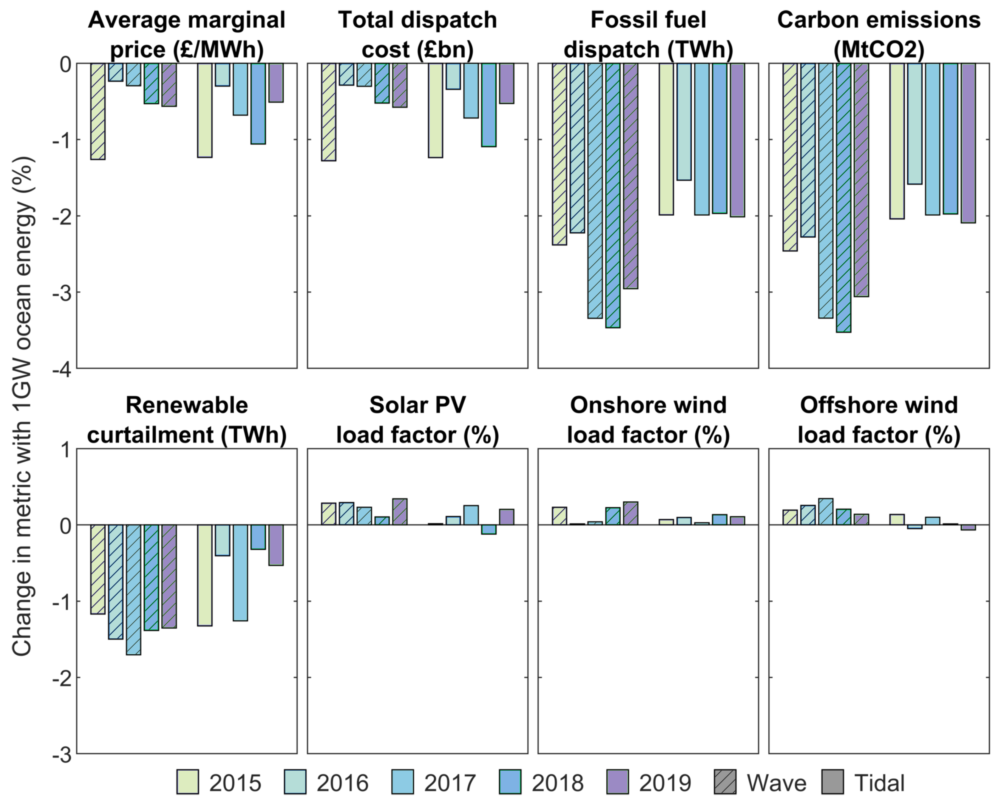
3.2.2. Switching in Ocean Energy

The overall premise of the modelling undertaken was to illustrate the impact of including ocean energy as part of the future generation mix. To reiterate, the ocean energy included is instead of some of the projected increase in offshore wind capacity, with the total renewable energy generation kept constant. The capacities in this section are not intended as predictions of how much ocean energy will be installed, but as examples to illustrate the impact of including ocean energy in the mix, and the variability of results depending on the input data year used. For reference, in the FES LTW 2030 scenario, 1 GW is 0.57% of the 176.81 GW total installed generation and 0.79% of the 126.89 GW of renewables [28].

Ocean energy, either wave or tidal steam, is shown to have a positive impact on all metrics considered in almost every case, as ocean energy may be available at different times from other renewable technologies. The impact on the same metrics as before from incorporating 1 GW of ocean energy is shown in Figure 8. To facilitate comparison, this is plotted as the change in the metric for the sensitivity cases with 1 GW wave or tidal energy relative to the baseline with no ocean energy, noting that this baseline differs between years, as shown in Figure 7.

As with the baseline case, there is a clear relationship between average marginal price and total dispatch cost, and between fossil fuel dispatch and carbon emissions, with variation depending on the year of input data. However, within these results, the year with the greatest change in dispatch cost does not necessarily reflect the largest reduction in emissions, given the complexity of the power system modelled and the specific hourly patterns of demand and renewable availability. The 2015 data has the greatest reduction in dispatch cost for both the wave and tidal sensitivity cases, although this is not reflected in the change in carbon emissions The change in the first five metrics can be considered significant at the 5% level; results tabulated in

Table A7. p-values for each metric and technology.

Technology	Average Market Price (GBP/MWh)	Total Dispatch Cost (Billion GBP)	Fossil Fuel Dispatch (TWh)	Carbon Emissions (MtCO2)	Renewable Curtailment (TWh)	Solar PV Load Factor (%)	Onshore Wind Load Factor (%)	Offshore Wind Load Factor (%)
Wave	0.0311	0.0307	0.0001	0.0001	0.0002	0.0035	0.0459	0.0031
Tidal	0.0102	0.0092	0.0001	0.0002	0.0337	0.2485	0.0074	0.5366

.

The modelling suggests that including ocean energy does not have a big impact on the load factor for other intermittent renewable generation. The greatest change is seen for the 2017 data wave sensitivity, where the load factor for offshore wind increases to 42.10% from 41.96%, an absolute difference of just 0.14 percentage points, or a relative change of 0.34%.

For many of the sensitivity cases presented in Figure 8, wave performs more favourably than tidal, resulting from the better matching of the wave resource with demand over the year, as discussed in Section 3.1.1.

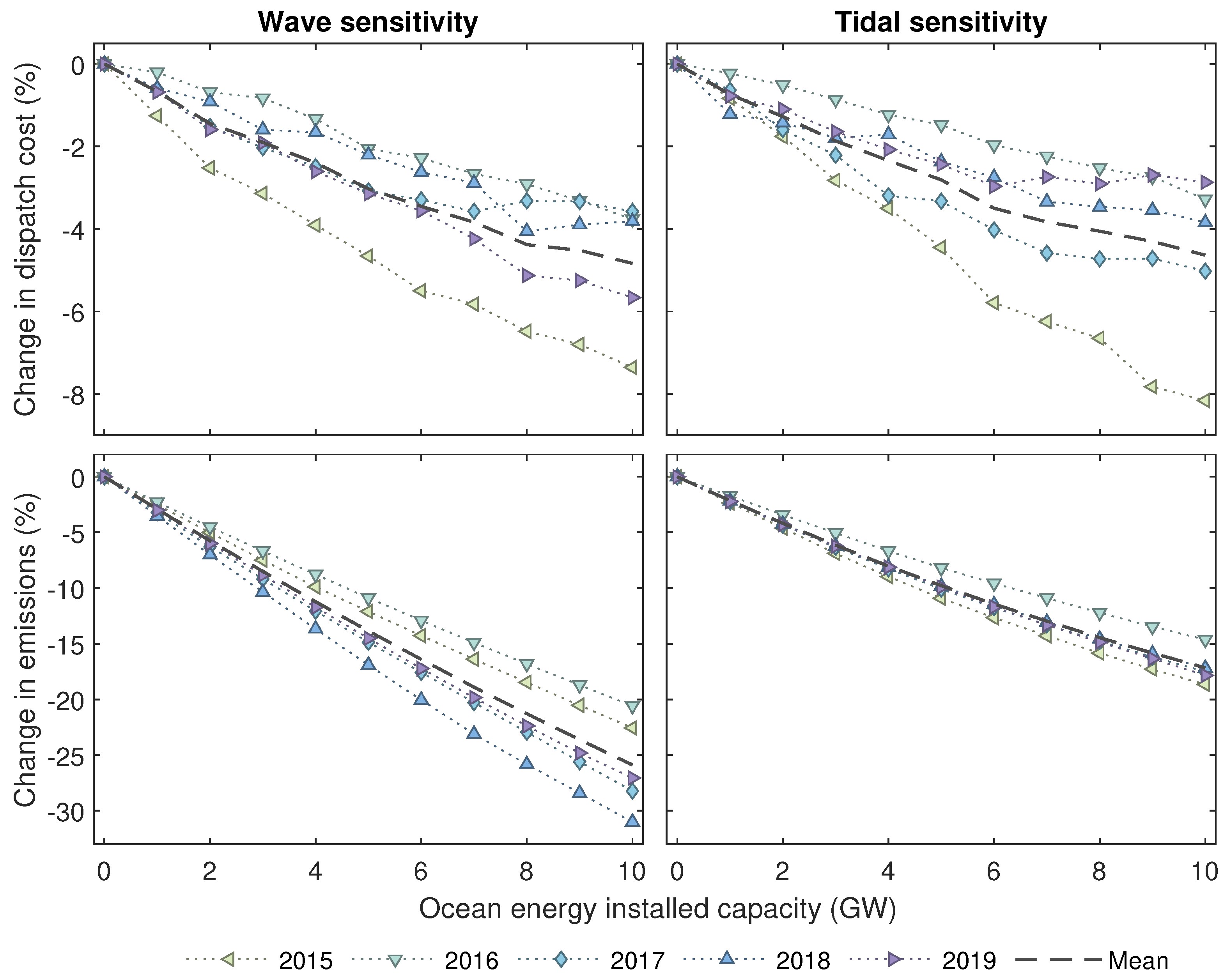
As also shown in [27], these trends continue with an increasing penetration of ocean energy. Scenarios including up to 10 GW of either wave or tidal steam as part of the generation mix are shown in Figure 9, for total dispatch cost and carbon emissions.

Carbon emissions reduce proportionally with installed ocean energy, also dependent on input data year. The greatest change is the 2018 input data with 10 GW wave showing a reduction of 31%, while the 2015 data for 10 GW tidal was 18.7%. This also shows there is less variation between input data years for tidal stream ($\begin{array}{c}-14.6\\ -18.7\end{array}\%$) than for wave ($\begin{array}{c}-20.6\\ -31.0\end{array}\%$), as tidal is more consistent between years, as discussed in Section 3.1.

The change in dispatch cost is less consistently linked to the ocean energy capacity. This is because displacing any fossil fuel dispatch reduces emissions, but costs only change when a cheaper technology sets the marginal price, which may not happen in all periods.

3.3. Summary of Results

The results show the benefits of a more diverse range of electricity generation, including ocean energy, in the context of the variability in electricity demand and intermittent renewable resources.

They illustrated the potential variation in GB electricity demand and the availability of renewable generation, depending on the year of input data used. Even with the small sample of five years (2015–2019), total demand varies +3.6/−2.0% relative to the mean of this period, and availability of intermittent renewables +9.0/−7.1%. The outputs from the dispatch model can be even more sensitive to the year of input data chosen, with dispatch costs varying +21/−13% and carbon emissions +45/−27%.

Sensitivity analysis cases were used to explore the impact of using ocean energy (wave or tidal stream) as part of the generation mix. Benefits were seen across all eight metrics considered for almost every year of input data. The resulting change from using 1 GW of ocean energy was −0.2/−1.3% on costs and −2.3/−3.5% on carbon emissions, equating to a saving of 36–177 million GBP on total dispatch cost and 61–140 ktCO₂, depending on the year of input data considered. Renewable curtailments dropped −0.3/−1.7%, with the load factor for other renewable generation varying +0.3/−0.1%, although this equates to a relatively minor +0.08/−0.03 percentage point difference in output.

While these sensitivity case results show a clear benefit of including ocean energy as part of the future generation mix, quantification of this benefit is subject to the year of input data used in the modelling. This is a result of both the hourly electricity demand and the hourly availability of intermittent renewable generation being linked to the weather. A more diverse renewable generation mix is more likely to be available at times of high demand, thus lowering the requirement for expensive and polluting gas generation. While tides are decoupled from the weather, their availability fluctuates periodically; tidal stream energy will also only form a small part of the overall mix, and thus, these cases still exhibit variability depending on the year of input data.

3.4. Limitations and Further Work

This paper has started to explore the range of variability in GB electricity demand and availability of intermittent renewable generation, at an hourly timestep considering both variability within and between years. There is a more detailed discussion on the strengths and limitations of this type of model in the modelling framework paper [27], along with additional sensitivity analysis. As with all modelling, certain assumptions and exclusions need to be made around aspects that are not central to the main analysis, e.g., future changes to subsidy policies or to electricity and carbon markets.

Ocean energy, and wave energy in particular, is an emerging technology with many different concepts being developed [5]. Within our work, one wave technology has been used to produce a scenario of potential electricity generation from the wave resource; however, the trends for other technologies are expected to be broadly similar. This work includes an implicit assumption that ocean energy technology develops to a sufficient level of maturity to be installed at scale.

The approach followed in this work could also be applied to other countries or regions, and it is likely these would also exhibit sensitivity to the year of input data used. However, differences in the energy systems markets, including demand patterns (climate, weather, cultural, etc.), the mix and availability of different generation technologies, and their costs, all preclude generalisation of specific results.

The dispatch model results in Section 3.2 are from a simplified representation of the transmission system, and do not include the impact of network constraints. As shown in [27], transmission constraints would impact the results, particularly when significant tidal energy (>6 GW) is included within the mix, due to the location of significant tidal resource in the north of Scotland. This would apply to all forms of intermittent renewable generation; however, future grid upgrade works and/or energy storage would be expected before the rollout of significantly more capacity in constrained regions.

Other studies have investigated the use and uncertainties around increased use of energy storage (e.g., [47,48]; however, these do not include ocean energy as part of the generation mix. Conversely, this work includes ocean energy, but with the caveat of a simplified representation of energy storage.

It was also not within the scope of this work to investigate the spatio-temporal variability of intermittent renewable generation. The availability profiles were developed for a geographically representative set of sites, but the temporal variability of each site was not assessed. This could, however, be an interesting extension of this work.

The Earth’s climate is changing ever more rapidly, with more frequent and extreme weather events affecting electricity supply and demand, although the impacts of this are still uncertain (e.g., [15,49,50]. To avoid compounding uncertainties, this was not considered within the scope of the work. Therfore, long-term changes in the resource, such as wind or wave conditions resulting from climate change, were not modelled in this work. Similarly, many other factors, such as economics, government policies, development of infrastructure and technologies, etc., will have some influence, but these have not been included in the study.

This work only considered a small sample (five years) of data. While not fully representative, this does highlight the potential variability, while balancing the effort required to produce input data for additional years and compute corresponding dispatch model cases. Using specific years of matching demand and availability data for analysis does limit the number of data points that can be modelled, based on the length of record available and considered still representative, five in this case or twelve in [26]. Conversely, using synthetic data with a Monte Carlo type analysis often uses 1000 or more runs, but may fail to capture correlations between the sources. Future work could expand on the investigation and results presented here with a more robust statistical analysis of the variability over a longer period. This could include multi-scale spectral analysis or other climate science tools.

4. Conclusions

This paper produces quantitative results to explore the power system benefits of ocean energy (wave and tidal stream) within a future energy scenario for the GB grid. Ocean energy can be available at different times to other variable renewable technologies such as wind and solar, and thus, including ocean energy can offer power systems benefits by improving supply–demand balancing on annual/subannual timeframes.

Both electricity demand and renewable generation availability are linked to the weather conditions. As a result, when modelling hourly dispatch, it is important to use a consistent year for the demand and availability input data. However, weather conditions are variable, both year-on-year and within the year. This work starts to quantify the benefits of ocean energy in the context of this variability, by using five years of consistent input data (2015–2019) and assessing the impact on results.

For these input data years, annual electricity demand in GB varied by a few percent, ±4% relative to the average of the period. Modelled availability for solar PV and tidal stream exhibits less variability to input data year, under ±2%. Wave, offshore wind, and in particular onshore wind, show greater variability of ±4–9%.

The timing and pattern of peak demand varies considerably between years, as does the corresponding availability of renewable generation at these times. Therefore, when considering the dispatch model output metrics, fossil fuel dispatch and carbon emissions are particularly sensitive to the year of input data, varying +45/−27%. Average marginal price and total dispatch cost showed about half this sensitivity.

Inclusion of ocean energy within the future generation mix shows benefits across a range of metrics for every input data year modelled. Including 1 GW of wave or tidal power as part of the same total renewable energy mix showed reductions in total dispatch cost of 36–177 million GBP (0.2–1.3%) and a saving in carbon emissions of 61–140 ktCO₂ (2.3–3.5%). For context, 1 GW is 0.57% of total and 0.79% of renewable generation capacity.

Key conclusions from this work are that the variability of both demand and generation profiles can have a significant impact on energy system modelling results and that diversifying the renewable energy mix by including wave and tidal can produce energy system benefits, reducing cost and carbon emissions in high renewable power systems. These findings are important for energy systems modellers looking to better represent renewable profiles and for policy and decision makers looking to understand the limitations and requirements of energy systems modelling results.

Finally, regarding recommendations for best practise in future modelling studies, they should not just consider one ‘average’ year of data in isolation; it is preferable to model multiple consecutive years to give a better understanding of the impact and their variability. It is also important to use consistent input data years to capture the correlations between demand, resource availability, and the weather.