A Comprehensive Simplified Algorithm for Heat Transfer Modeling of Medium-Deep Borehole Heat Exchangers Considering Soil Stratification and Geothermal Gradient

Abstract

Medium-deep borehole heat exchanger (BHE) systems represent an emerging form of ground source heat pump technology. Their heat transfer process is significantly influenced by geothermal gradient and soil stratification, typically simulated using segmented finite line source (SFLS) models. However, this approach involves computationally intensive procedures that hinder practical engineering implementation. Building upon an SFLS model adapted for complex geological conditions, this study proposes a comprehensive simplified algorithm: (1) For soil stratification: A geothermally-weighted thermal conductivity method converts layered heterogeneous media into an equivalent homogeneous medium; (2) For geothermal gradient: A temperature correction method establishes fluid temperatures under geothermal gradient by superimposing correction terms onto uniform-temperature model results (g-function model). Validated through two engineering case studies, this integrated algorithm provides a straightforward technical tool for heat transfer calculations in BHE systems.

1. Introduction

Heating and cooling are fundamental operational requirements for any type of building to maintain indoor spaces in a thermally comfortable environment. The demand for thermal energy in buildings has been increasing dramatically year by year. In the United States, renewable energy accounted for only 9% of total energy consumption in 2005, but this proportion increased to 13.2% by 2014. Research [1] predicts it will reach 18% by 2040.

Geothermal energy is recognized as a significant renewable energy source alongside solar, wind, and hydro power. Due to the widespread existence of geothermal gradients worldwide, the abundant thermal energy from deep underground can be utilized for direct heating or as a heat source for heat pump systems, providing clean heating for buildings [2].

Currently, geothermal energy harnesses the Earth’s temperature near the surface (shallow geothermal energy) or by drilling deeper boreholes (deep geothermal energy). Geothermal systems can efficiently provide heating/cooling through direct heating or via heat pumps coupled with shallow or deep borehole heat exchangers, demonstrating immense potential. Compared to shallow borehole heat exchange systems, deep borehole heat exchange systems offer higher thermal capacity [3] (generally 10 times greater than shallow systems), smaller installation footprint [4], faster thermal recovery after heat extraction [3], and ensure stable heating over extended periods (typically 20 years or more) [5].

Several highly successful engineering applications of deep borehole heat exchange systems have been implemented in locations such as Xi’an [6,7] and Jilin [8]. Although these projects have achieved remarkable results in energy conservation and emission reduction, further theoretical research is needed to address fundamental aspects of deep borehole heating systems. A reliable computational model for deep borehole heat exchange systems is crucial for optimizing system design [9,10], studying intermittent heating modes [11], and analyzing multiple influencing factors [12,13]. Both geothermal gradients and subsurface stratification are critical geological conditions that significantly impact deep borehole heat exchange systems and must be carefully considered in modeling.

Subsurface stratification poses a major challenge in heat transfer modeling. Some studies indicate that for borehole heat exchanger models, if stratified soil conditions are simplified to homogeneous conditions [14], the output water temperature remains nearly identical. However, other studies, such as Perego et al. [15], show that simulation errors from ignoring stratification can reach up to 25%. Moreover, temperature errors due to stratified soil vary depending on the assigned thermal conductivity in different layers [16]. Karabetoglu et al. [17] suggest that the computational discrepancy between stratified and homogeneous soil models correlates with the variance in thermal conductivity across layers. Literature shows that most heat exchange models for boreholes in stratified soil rely on grid-based numerical solutions. Li et al. [3] developed a finite difference numerical model for deep borehole heat exchange systems under multi-layered soil conditions, discretizing soil with a uniform grid and solving it in MATLAB (2022b) with a 60 s time step and 10 m borehole spacing. Similar discretization methods have been applied in other studies [18,19]. Additionally, Finite Volume Method (FVM) and Finite Element Method (FEM) have provided effective computational models for simulating heat extraction in deep borehole systems under stratified soil and geothermal gradients. Beier et al. [20] attempted to extend traditional one-dimensional analytical models through a numerical approach by proposing a layer factor method. However, this method remains difficult to apply to more complex heat exchange scenarios in deep boreholes.

In practical applications of deep boreholes, the geothermal gradient in soil typically ranges from 0.02 K/m to 0.03 K/m, significantly affecting heat exchange. Existing shallow borehole heat exchange models often assume uniform soil temperature and heat flux distribution along the borehole depth. However, as borehole depth increases, the influence of geothermal gradients intensifies, leading to increasingly uneven heat flux distribution along the depth in deep borehole systems. This renders the uniformity assumption in shallow borehole models unsuitable for simulating deep borehole systems under geothermal gradients. For instance, simulations using Kelvin’s infinite line source model [21,22], which simplistically assumes uniform soil temperature, show errors exceeding 10% in estimated soil temperature distribution under a high geothermal gradient of 0.052 K/m compared to numerical models accounting for geothermal gradients.

To address geothermal gradient conditions in deep borehole systems, most researchers have developed numerical models, such as finite element models for borehole heat exchangers under varying geothermal gradients [23]. Similar numerical models can also be found in TRNSYS’s Type 557 module [24], which dynamically simulates borehole heat exchange systems with different configurations by assigning geothermal gradients. Holmberg et al. [25] constructed equations for circulating fluid and subsurface nodes within boreholes under deep geothermal gradients using the finite difference method. Fang et al. [18] employed a central difference scheme to establish node equations for subsurface regions and solved the difference equations using the chasing method to obtain temperature fields under geothermal gradients.

However, modeling deep borehole heat exchange systems often requires simultaneously addressing both soil stratification and geothermal gradients. Although both analytical and numerical models for deep borehole systems are evolving, analytical models lag significantly behind numerical ones. Pan et al. [26] and Fang et al. [27] developed analytical solutions for heat transfer in circulating fluids within boreholes, incorporating geothermal gradients based on a quasi-3D analytical model for double U-tube exchangers, and validated their accuracy. These analytical models can enhance computational efficiency to some extent. Yet, they do not account for the non-uniform heat flux distribution along the borehole depth. Luo et al. [28] proposed a Segmented Finite Line Source (SFLS) analytical model for deep borehole systems, offering an efficient and simple approach to handle geothermal gradients. However, this model only applies to homogeneous soil conditions. Later, Luo et al. [29] combined this analytical model with the composite medium method to develop a model accommodating both geothermal gradients and soil stratification, discretizing space (depth) and time during solving. Nevertheless, this method demands substantial computational effort for deep boreholes and long-term simulations.

The above analysis reveals that research on heat transfer models for deep borehole heat exchange systems predominantly focuses on numerical models, with limited development of analytical models. For numerical models, separate modeling is required for different deep borehole heat transfer problems, grid settings must be carefully designed, and lengthy computation times hinder widespread application. Analytical models often involve complex integrals and high computational costs due to intricate soil conditions, diminishing their advantage of rapid calculation. Therefore, developing a simplified algorithm with high computational efficiency holds significant importance for heat transfer calculations in medium-deep boreholes.

To address the aforementioned issues, this paper proposes a comprehensive analytical model for multi-borehole ground heat exchanger heat transfer that considers both soil stratification and the geothermal gradient. Utilizing the composite medium method to handle soil stratification and based on the superposition principle, this model establishes a segmented finite line source (SFLS) model under the combined influence of geothermal gradient and stratified soil. Furthermore, by analyzing the impact of soil stratification and geothermal gradient on borehole heat transfer calculations using this analytical model, a comprehensive simplified calculation method is proposed. This simplified method transforms the heat transfer calculation problem under stratified soil and geothermal gradient conditions into one under homogeneous soil conditions through fitted corrections and the g-function. Compared to the traditional SFLS model, which requires spatial and temporal discretization and computation of numerous integrals when handling geothermal gradients or soil stratification, our proposed comprehensive simplified method significantly reduces computation time. It achieves this by replacing stratified discretization with a depth-weighted average equivalent thermal conductivity based on the geothermal temperature profile, accounting for the geothermal gradient effect through a calculated temperature correction term, and combining this with the g-function approach for homogeneous models. The final method is validated against actual engineering projects.

2. Multi-Borehole Segmented Finite Line Source Model Under Soil Layering and Geothermal Gradient Conditions

2.1. Heat Transfer Model Outside the Borehole

For the ground heat exchanger model, the fluid heat exchange inside the borehole is first simplified as a line source, and then the heat transfer model outside the borehole is considered. The shallow segmented finite line source model is established under the condition of a medium with a uniform initial temperature distribution. Under the geothermal gradient, the initial temperature of the medium is linearly distributed; under soil layering, the thermal physical parameters of the medium also change with depth. Now, the segmented finite line source model is re-derived and improved. Since the analysis of the model considering both the geothermal gradient and soil layering is relatively complex, the two conditions are separated for individual analysis of the model, and finally, the two conditions are integrated into the heat transfer model outside the borehole.

2.1.1. Model Outside the Borehole Under Geothermal Gradient Conditions

Cimmino et al. [30] proposed a multi—borehole segmented finite line source heat transfer model under the condition of uniform initial soil temperature distribution. When considering the geothermal gradient, the soil temperature is usually considered to be linearly distributed. It can be proved that the temperature fields of the linearly—distributed geothermal field and the heat transfer of the ground heat exchanger are superimposable. Taking the soil condition with ground surface temperature $T_g$ and geothermal gradient $g_d$ as an example (where initial soil temperature is $T_0\left(z\right)=gd\cdot z+Tg$, with $z$ being soil depth): In a borehole field with $n_b$ boreholes of arbitrary size and location, each borehole has a radius of $r_b$, a length of $H$, is at a distance of $D_i$ from the ground surface, and has a location coordinate of $\left(x_i,y_i\right)$. The thermal conductivity of the soil is $k_s$, the thermal diffusivity is ${\alpha }_s$, and the initial soil temperature is $T_0$. The calculation formula for the temperature response of the borehole—wall on each borehole segment is as follows:

$$T_{b,j,v}\left(t_k\right)=-{\displaystyle \sum _{p=1}^k{\displaystyle \sum _{i=1}^{n_b}{\displaystyle \sum _{u=1}^{n_q}\frac{Q_{i,u}\left(t_p\right)-Q_{i,u}\left(t_{p-1}\right)}{2\pi k_s}\cdot h_{i\to j,u\to v}\left(t_p-t_{p-1}\right)+T_0\left(\frac{v-0.5}{n_q}\cdot H\right)}}}$$

(1)

$$\begin{array}{cc}\hfill h_{(i\to j,u\to v)}(t_k)=& {\displaystyle \frac{1}{2H_{(j,v)}}}{\displaystyle {\int }_{1/\sqrt{4{\alpha }_{\mathrm{s}}t}}^{\infty }exp(-{d_{ij}}^2{s}^2)[ierf((D_{(j,v)}-D_{(i,u)}+H_{(j,v)})s)}\hfill \\ & -ierf(s(D_{(j,v)}-D_{(i,u)}))+ierf((D_{(j,v)}-D_{(i,u)}-H_{(i,u)})s)\\ & -ierf((D_{(j,v)}-D_{(i,u)}+H_{(j,v)}-H_{(i,u)})s)+ierf((D_{(j,v)}+D_{(i,u)}+H_{(j,v)})s)\\ & -ierf(s(D_{(j,v)}+D_{(i,u)}))+ierf((D_{(j,v)}+D_{(i,u)}+H_{(i,u)})s)\\ & -ierf((D_{(j,v)}+D_{(i,u)}+H_{(j,v)}+H_{(i,u)})s)]\end{array}$$

(2)

$$ierf\left(X\right)=X\cdot erf\left(X\right)-{\displaystyle \frac{1}{\sqrt{\pi }}}\left(1-e^{-X^2}\right)$$

(3)

$$d_{ij}=\left\{\begin{array}{cc}{r}_b& ,i=j\\ \sqrt{{\left(x_i-x_j\right)}^2+{\left(y_i-y_j\right)}^2}& ,i\ne j\end{array}\right.$$

(4)

where $T_{b,j,v}\left(t_k\right)$ is the temperature response of the borehole—wall of the $v$-th segment of the $j$-th borehole after time $t_k$; $T_0\left({\displaystyle \frac{v-0.5}{n_q}}\cdot H\right)$ represents the initial average soil temperature of the $v$-th segment of the borehole; $d_{ij}$ is the distance between the $i$-th borehole with the coordinate $\left(x_i,y_i\right)$ and the $j$-th borehole with the coordinate; $h_{i\to j,u\to v}$ is the inter—segment temperature—response coefficient of the $u$-th segment of the $i$-th borehole to the $v$-th segment of the $j$-th borehole; $H_{i,u}$ and $D_{i,u}$ are the length and burial depth of the $u$-th segment of the $i$-th borehole.

2.1.2. Model Outside the Borehole Under Soil Layering

Based on the above—mentioned heat—transfer model outside the borehole of the segmented finite line source considering the geothermal gradient, continue to consider the case where the deep borehole is buried in multiple layers of strata, that is, the model outside the borehole under soil layering. Two representative methods can be found in the literature.

One is the use of the Laplace and numerical inverse Laplace methods [29]. This method cannot be combined with the geothermal—gradient condition. The other method is the composite—medium method [31]. It calculates a set of equivalent thermal—physical parameters representing heat transfer through multiple underlying layers according to the different positions of the heat source and the calculation point. This method provides a very simple and effective way to deal with layering. This method has also been applied to the calculation of a single—hole coaxial—casing heat—exchange model [28]. Therefore, this composite—medium method is combined with the segmented finite line source model.

As shown in Figure 1a, in the segmented finite line source model under a homogeneous medium, the thermal responses between pipe segments at different spatial positions can be expressed only by using the same $k_s$ and ${\alpha }_s$. However, in the case of soil layering in Figure 1b, this is no longer applicable. Therefore, the composite—medium method is used to determine the composite thermal conductivity between segments. The composite—medium parameter values $\left(k_{comp},{\alpha }_{comp},k_{comp}^{*},{\alpha }_{comp}^{*}\right)$ are specifically determined by the specific strata passed by the line connecting the heat source and the calculation point. In Figure 1b, $S$ represents the distance passing through different strata, and the calculation is as follows:

$$\left\{\begin{array}{c}{\rho }_{comp}={\displaystyle \sum _{i=1}^N\frac{S_i}{{\displaystyle \sum S_i}}\times {\rho }_i}\\ k_{comp}={\displaystyle \frac{1}{{\displaystyle \sum _{i=1}^N\frac{S_i}{{\displaystyle \sum S_i}}\times \frac{1}{k_i}}}}\\ C_{comp}={\displaystyle \sum _{i=1}^N\frac{S_i{\rho }_i}{{\displaystyle \sum S_i{\rho }_i}}\times C_i}\\ {\alpha }_{comp}={\displaystyle \frac{k_{comp}}{{\rho }_{comp}{C}_{comp}}}\end{array}\right.$$

(5)

So for the segmented finite line source model under soil layering, the calculation of the inter—segment temperature response is modified from Equation (1) to Equation (7), where the composite—medium parameters $k_{comp}$ and ${\alpha }_{comp}$ are determined by the spatial position of the calculation point and the actual heat source, and $k_{comp}^{*}$ and ${\alpha }_{comp}^{*}$ are the composite—medium parameters of the virtual heat source at the corresponding spatial point.

$$T_{b,j,v}\left(t_k\right)=-{\displaystyle \sum _{p=1}^k{\displaystyle \sum _{i=1}^{n_b}{\displaystyle \sum _{u=1}^{n_q}\frac{Q_{i,u}\left(t_p\right)-Q_{i,u}\left(t_{p-1}\right)}{2\pi k_{comp}}\cdot h_{i\to j,u\to v}^{*}\left(t_k-t_{p-1}\right)+T_0\left(\frac{v-0.5}{n_q}\cdot H\right)}}}$$

(6)

By combining the above—mentioned composite—medium method with the segmented finite line source model under the geothermal gradient, the heat—transfer model outside the borehole of the medium—and deep—buried ground heat exchanger under the background of soil layering and the geothermal gradient is established. At this time, it is also necessary to establish a heat—transfer model of the fluid inside the borehole to provide the fluid—temperature field at each time node and the heat—exchange amount along the borehole wall.

2.2. Heat Transfer Model of the Fluid Inside the Borehole

The fluid heat transfer model accurately simulates the circulating fluid inside the borehole. The fluid heat exchange inside the borehole can be considered a steady—state process during operation because the water—temperature field can reach a thermal—equilibrium state within a relatively short time range. This treatment method has been applied in many other models of fluid heat transfer inside the borehole of ground heat exchangers, such as the equivalent—diameter model [32], the MISOS model [33], and the CaRM model [34]. Based on the steady—state heat—exchange process of the fluid inside the borehole, Cimmino et al. [30] proposed a model for the fluid heat exchange inside the borehole of a U-tube in the segmented model. Although the heat—exchange characteristics of the U-tube and the coaxial casing are different, they can adopt the same basic equations. Therefore, the calculation formula for the fluid heat exchange inside the borehole of the coaxial casing in the segmented model is as follows:

$$\begin{array}{cc}\hfill {\displaystyle \frac{Q_{i,u}\left(t_k\right)}{m{c}_p}}{\displaystyle \frac{H}{n_q}}=& T_{f1,i,0}\left(t_k\right)\left[\left(X_1\left({\displaystyle \frac{u}{n_q}}\right)-X_1\left({\displaystyle \frac{u-1}{n_q}}\right)\right)-{\displaystyle \frac{X_1\left(1\right)}{X_2\left(1\right)}}\left(X_2\left({\displaystyle \frac{u}{n_q}}\right)-X_2\left({\displaystyle \frac{u-1}{n_q}}\right)\right)\right]\hfill \\ & +{\displaystyle \sum _{v=1}^u{T}_{b,i,v}\left(t_k\right)}\left(X_3\left({\displaystyle \frac{u-v+1}{n_q}}\right)-X_3\left({\displaystyle \frac{u-v}{n_q}}\right)\right)\\ & -{\displaystyle \sum _{v=1}^{u-1}{T}_{b,i,v}\left(t_k\right)}\left(X_3\left({\displaystyle \frac{u-v}{n_q}}\right)-X_3\left({\displaystyle \frac{u-v-1}{n_q}}\right)\right)\\ & -{\displaystyle \frac{X_2\left(\frac{u}{n_q}\right)-X_2\left(\frac{u-1}{n_q}\right)}{X_2\left(1\right)}}{\displaystyle \sum _{v=1}^{n_q}{T}_{b,i,v}\left(t_k\right)}\left(X_3\left({\displaystyle \frac{u-v+1}{n_q}}\right)-X_3\left({\displaystyle \frac{u-v}{n_q}}\right)\right)\end{array}$$

(7)

$$X_1\left({\displaystyle \frac{u}{n_q}}\right)=f_1\left({\displaystyle \frac{u}{n_q}}\right)+f_2\left({\displaystyle \frac{u}{n_q}}\right)=\exp \left({\beta }^{\prime }{\displaystyle \frac{u}{n_q}}\right)\left(\cosh \left({\gamma }^{\prime }{\displaystyle \frac{u}{n_q}}\right)-{\displaystyle \frac{{\beta }_1^{\prime }+{\beta }_2^{\prime }}{2{\gamma }^{\prime }}}\sinh \left({\gamma }^{\prime }{\displaystyle \frac{u}{n_q}}\right)\right)$$

(8)

$$X_2\left({\displaystyle \frac{u}{n_q}}\right)=f_3\left({\displaystyle \frac{u}{n_q}}\right)-f_2\left({\displaystyle \frac{u}{n_q}}\right)=\exp \left({\beta }^{\prime }{\displaystyle \frac{u}{n_q}}\right)\left(\cosh \left({\gamma }^{\prime }{\displaystyle \frac{u}{n_q}}\right)+{\displaystyle \frac{{\beta }_1^{\prime }+{\beta }_2^{\prime }}{2{\gamma }^{\prime }}}\sinh \left({\gamma }^{\prime }{\displaystyle \frac{u}{n_q}}\right)\right)$$

(9)

$$X_3\left({\displaystyle \frac{u}{n_q}}\right)={\displaystyle \frac{1}{H}}\exp \left({\beta }^{\prime }{\displaystyle \frac{u}{n_q}}\right){\displaystyle \frac{{\beta }_1^{\prime }+{\beta }_2^{\prime }}{{\gamma }^{\prime }}}\sinh \left({\gamma }^{\prime }{\displaystyle \frac{u}{n_q}}\right)$$

(10)

$$f_1\left({\displaystyle \frac{z}{H}}\right)=\exp \left({\beta }^{\prime }{\displaystyle \frac{z}{H}}\right)\left[\cosh \left({\gamma }^{\prime }{\displaystyle \frac{z}{H}}\right)-\delta \sinh \left({\gamma }^{\prime }{\displaystyle \frac{z}{H}}\right)\right]$$

(11)

$$f_2\left({\displaystyle \frac{z}{H}}\right)=\exp \left({\beta }^{\prime }{\displaystyle \frac{z}{H}}\right){\displaystyle \frac{{\beta }_{12}^{’}}{{\gamma }^{\prime }}}\sinh \left({\gamma }^{\prime }{\displaystyle \frac{z}{H}}\right)$$

(12)

$$f_3\left({\displaystyle \frac{z}{H}}\right)=\exp \left({\beta }^{\prime }{\displaystyle \frac{z}{H}}\right)\left[\cosh \left({\gamma }^{\prime }{\displaystyle \frac{z}{H}}\right)+\delta \sinh \left({\gamma }^{\prime }{\displaystyle \frac{z}{H}}\right)\right]$$

(13)

$$f_4^{\prime }\left({\displaystyle \frac{z}{H}}\right)=\exp \left({\beta }^{\prime }{\displaystyle \frac{z}{H}}\right)\left[{\beta }_1^{\prime }\cosh \left({\gamma }^{\prime }{\displaystyle \frac{z}{H}}\right)-\left(\delta {\beta }_1^{\prime }+{\displaystyle \frac{{\beta }_2^{\prime }{\beta }_{12}^{\prime }}{{\gamma }^{\prime }}}\right)\sinh \left({\gamma }^{\prime }{\displaystyle \frac{z}{H}}\right)\right]$$

(14)

$$f_5^{\prime }\left({\displaystyle \frac{z}{H}}\right)=\exp \left({\beta }^{\prime }{\displaystyle \frac{z}{H}}\right)\left[{\beta }_2^{\prime }\cosh \left({\gamma }^{\prime }{\displaystyle \frac{z}{H}}\right)+\left(\delta {\beta }_2^{\prime }+{\displaystyle \frac{{\beta }_1^{\prime }{\beta }_{12}^{\prime }}{{\gamma }^{\prime }}}\right)\sinh \left({\gamma }^{\prime }{\displaystyle \frac{z}{H}}\right)\right]$$

(15)

where ${\beta }_1^{\prime }={\displaystyle \frac{\xi H}{m{c}_p{R}_b}}$, ${\beta }_2^{\prime }={\displaystyle \frac{\left(1-\xi \right)H}{m{c}_p{R}_b}}$, ${\beta }_{12}^{\prime }={\displaystyle \frac{H}{m{c}_p{R}_{12}}}$ are the dimensionless thermal conductivities of the borehole, ${\beta }_1^{\prime }={\displaystyle \frac{{\beta }_2^{\prime }-{\beta }_1^{\prime }}{2}}$, ${\gamma }^{\prime }=\sqrt{{\left({\beta }_1^{\prime }+{\beta }_2^{\prime }\right)}^2/4+{\beta }_{12}^{\prime }\left({\beta }_1^{\prime }+{\beta }_2^{\prime }\right)}$, $\delta ={\displaystyle \frac{1}{{\gamma }^{\prime }}}\left({\beta }_{12}^{\prime }+{\displaystyle \frac{{\beta }_1^{\prime }+{\beta }_2^{\prime }}{2}}\right)$, and $z$ is the depth from the ground surface. $R_b$ is the borehole thermal resistance, $R_{12}$ is the short—circuit thermal resistance between the annulus tube and the central tube. When the annulus tube is used as the fluid inlet, $\xi =1$; when the central tube is used as the fluid inlet, $\xi =0$. Meanwhile, when $z=0$, the outlet fluid temperature $T_{f2,i,0}\left(0,t\right)$ is given by the following formula:

$$T_{f2,i,0}\left(t_k\right)=T_{f1,i,0}\left(t_k\right)\cdot {\displaystyle \frac{f_1\left(1\right)+f_2\left(1\right)}{f_3\left(1\right)-f_2\left(1\right)}}+{\displaystyle \frac{1}{H}}{\displaystyle \sum _{v=1}^{n_q}\frac{T_{b,i,v}\left(t_k\right)}{f_3\left(1\right)-f_2\left(1\right)}d{z}^{″}}$$

(16)

Equation (7) is the calculation formula for the heat transfer per unit length between the fluid and the borehole wall on each borehole segment in the segmented borehole—inner model. The calculation boundary conditions of this formula are coupled with the segmented model outside the borehole mentioned above.

2.3. Model Validation

Integrate the model outside the borehole and the model inside the borehole, and combine Equations (6) and (7) into one algorithm. At the same time, by giving the total heat exchange of the borehole field Q or the fluid inlet temperature $T_{f1,i,0}\left(t_k\right)$, a complete multi-borehole segmented finite line source model under soil layering and geothermal gradient conditions is established:

It should be noted that: (1) At the beginning of the simulation, the total heat exchange change curve of the borehole field or the borehole inlet temperature change curve of the borehole field should be given to the model as the simulation condition input; (2) The model needs to divide the time step only when the heat exchange and the inlet temperature change are input. Therefore, the division of the time step only needs to meet the needs of the input curve change to reduce the model calculation time; (3) The initial wall temperature of the borehole wall is the initial soil temperature at the corresponding depth.

The proposed analytical model comprehensively accounts for the geothermal gradient and soil stratification, integrating them with the multi-bore segmented finite line source (SFLS) model. Its accuracy and effectiveness require validation. Using an actual medium-deep ground source heat pump system project in Xi’an as a case study, the results from the segmented finite line source model are compared with actual operational data [28] and numerical solution results from TRNSYS. In this project, operational data for the ground source heat pump system were collected through field testing and analysis of monitoring data. The geological parameters are listed in

Table 1. Geological parameters.

Soil Type	Depth (m)	Thermal Conductivity (W/m·K)	Density (kg/m3)	Specific Heat Capacity (J/kg·K)
Clay	0–636	1.8	1780	1379
Mudstone	636–1198	2.6	2030	1450
Medium—grained Sand	1198–1910	3.5	1510	1300
Sandstone	1910–3000	5.3	2600	878

, and the system and model parameters are provided in

Table 2. System and model parameters.

Model Parameter	Value
Borehole Depth (m)	2000
Number of Ground Heat Exchangers	18
Central Tube Specification (mm)	125 × 11.4
Annulus Tube Specification (mm)	193.7 × 8.33
Central Tube Thermal Conductivity (W/m·K)	0.4
Annulus Tube Thermal Conductivity (W/m·K)	41
Water Thermal Conductivity (W/m·K)	0.618
Water Specific Heat Capacity (J/kg·K)	4174
Backfill Material Thermal Conductivity (W/m·K)	1.5
Ground Surface Temperature (°C)	10
Geothermal Gradient (°C/m)	0.03

.

Using these parameters, the operational performance throughout the 1100-h heating season was simulated in the model. TRNSYS simulations utilized the measured inlet temperature as the initial condition. As shown in Figure 2, the simulated water temperatures from the actual measurements, TRNSYS, and the analytical model are compared. The results demonstrate good agreement between the analytical model simulations and both the measured data and TRNSYS simulations. Specifically: The RMSE between the analytical model and measured data is 1.02 °C for inlet temperature and 0.91 °C for outlet temperature. The RMSE between the analytical model and TRNSYS simulations is 1.02 °C for inlet temperature and 0.83 °C for outlet temperature.

3. Influence Analysis of Heat Transfer Calculation Under Geothermal Gradient and Soil Layering

3.1. Impact of Geothermal Gradient on BHE Temperature Distribution

During the heat exchange process between medium-deep BHEs and the soil, the geothermal gradient leads to significant temperature differences between the upper and lower soil layers. For example, over a depth difference of 2000 m, the soil temperature difference can reach 60 °C. This temperature distribution along the depth causes substantial differences in the heat exchange conditions between the fluid and the soil at different depths, further exacerbating the non-uniform heat exchange along the borehole depth in deep BHE systems. Compared to the heat flux distribution under uniform soil temperature conditions, the geothermal gradient significantly alters the heat exchange characteristics of medium-deep BHEs.

Controlling the average soil temperature to be the same, we compare the temperature change at the borehole wall and the heat exchange rate per meter at various depths under constant heat extraction rates for BHEs, considering both geothermal gradient and uniform temperature conditions. Calculations are performed for 5 different BHE depths under both conditions. The BHE system parameters are listed in

Table 3. BHE system parameters.

Model Parameter	Value
Borehole Depth (m)	2500
Central Pipe Specification (mm)	$110\times 4$
Annular Pipe Specification (mm)	$178\times 4.5$
Central Pipe Thermal Conductivity ($\mathrm{W}/\mathrm{m}\cdot \mathrm{K}$)	0.04
Annular Pipe Thermal Conductivity ($\mathrm{W}/\mathrm{m}\cdot \mathrm{K}$)	53
Water Thermal Conductivity ($\mathrm{W}/\mathrm{m}\cdot \mathrm{K}$)	0.618
Water Specific Heat Capacity ($\mathrm{J}/\mathrm{kg}\cdot \mathrm{K}$)	4174
Backfill Material Thermal Conductivity ($\mathrm{W}/\mathrm{m}\cdot \mathrm{K}$)	3

, with a BHE flow rate of 2 kg/s.

Figure 3 shows the calculation results from the SFLS analytical model. The figures use logarithmic time $\ln \left(t/t_s\right)=-7.8$ (where $t_s$ is the characteristic time, calculated by Equation (1)). They depict the variation of borehole wall temperature and heat exchange rate per meter along the depth when the constant heat extraction rate per meter $Q=40 \mathrm{W}/\mathrm{m}$ is applied. The actual time corresponding to this logarithmic time at different depths ranges from 7 months to 2 years. The results show that: The borehole wall temperature under uniform temperature conditions exhibits an approximately linear distribution. The borehole wall temperature under geothermal gradient conditions shows a certain non-linear distribution, and this non-linearity becomes more pronounced with increasing BHE depth. The heat exchange rate per meter under uniform temperature conditions is relatively uniform along the depth direction. The heat exchange rate per meter under geothermal gradient conditions gradually increases along the depth direction, showing significant non-uniformity.

Figure 4 displays the variation of the average borehole wall temperature over time for BHEs at different depths, calculated using the SFLS model, under both uniform temperature and geothermal gradient (0.03 °C/m) conditions in the soil. It can be seen that the average borehole wall temperature response along the depth under the two temperature backgrounds is almost identical over a considerable time range. At logarithmic time $\ln \left(t/t_s\right)<-4$, the relative error is less than 2%. For depths above 1000 m, the time t corresponding to $\ln \left(t/t_s\right)<-4$ far exceeds 60 years. Therefore, in practical operation, the calculated average temperature response along the depth at the borehole wall can be considered identical during the system’s service life.

3.2. Impact of Thermal Conductivity and Heat Capacity in Stratified Soil on Heat Transfer Calculation

Under the influence of soil stratification, different soil layers at varying depths have different thermal properties (such as thermal conductivity and heat capacity), leading to changes in the heat exchange behavior of the BHE in different strata. This causes errors when calculating the temperature response of BHEs in stratified soil using homogeneous soil thermal property parameters.

We now investigate the magnitude of the impact of stratified soil thermal conductivity and heat capacity on BHE heat transfer calculation under geothermal gradient conditions. Taking a single-borehole BHE with the configuration in Table 3 as an example, operating in soil with a geothermal gradient of 0.03 °C/m and surface temperature of 15 °C, the SFLS model calculates the temperature response for a heat extraction rate of 120 W/m and a flow rate of 6.39 kg/s. We compare the calculated fluid temperature differences under four calculation methods for stratified soil, as shown in

Table 4. Soil thermal property parameters for each case.

	Thermal Conductivity (W/m·K)	Soil Heat Capacity (J/kg·K)	Soil Depth (m)
Case 1	1.5	$0.89\times {10}^6$	0–600
	2.5	$1.41\times {10}^6$	600–1200
	3.5	$1.80\times {10}^6$	1200–1800
	4.5	$2.24\times {10}^6$	1800–3000
Case 2	1.5	$1.61\times {10}^6$	0–600
	2.5		600–1200
	3.5		1200–1800
	4.5		1800–3000
Case 3	3.06	$0.89\times {10}^6$	0–600
		$1.41\times {10}^6$	600–1200
		$1.80\times {10}^6$	1200–1800
		$2.24\times {10}^6$	1800–3000
Case 4	3.06	$1.61\times {10}^6$	0–3000

. Case 1 serves as the standard control group, using no simplification assumptions for the thermal conductivity or heat capacity of the stratified soil. Cases 2, 3, and 4 apply simplified average treatments to either the thermal conductivity or heat capacity of the stratified soil and calculate the results, comparing them to Case 1.

The homogeneous thermal conductivity and homogeneous volumetric heat capacity for Cases 2–4 are calculated using depth-weighted averaging. In an n-layer soil with layer thickness $h_i$ and thermal conductivity $k_{s,i}$, the homogeneous thermal conductivity for a BHE depth H is calculated by Equation (17), and the homogeneous volumetric heat capacity is calculated by Equation (18).

$$k_m={\displaystyle \frac{{\displaystyle {\sum }_{i=1}^n{h}_i\cdot k}}{H}}$$

(17)

$${\left(\rho c\right)}_m={\displaystyle \frac{{\displaystyle {\sum }_{i=1}^n{h}_i\cdot {\left(\rho c\right)}_i}}{H}}$$

(18)

Figure 5 show the fluid outlet temperatures for the four cases and the relative fluid temperature differences compared to Case 1. It can be seen that: Case 2 has the smallest relative temperature difference compared to Case 1, and this relative fluid temperature difference gradually decreases with increasing heat transfer time. The average relative fluid temperature difference is 0.83 °C. The average relative fluid temperature difference for Case 3 compared to Case 1 is 4.33 °C. The average relative fluid temperature difference for Case 4 compared to Case 1 is 5.10 °C, and this difference gradually increases over time. This indicates that when calculating the temperature response of BHEs in stratified soil under geothermal gradient conditions, the error introduced by a simple homogeneous assumption for the stratified soil heat capacity is relatively small. In contrast, the error introduced by a homogeneous assumption for the stratified soil thermal conductivity is significant. Therefore, to simplify the heat transfer calculation for BHEs in stratified soil, a homogeneous assumption can be applied to the soil heat capacity, but the layered nature of the soil thermal conductivity must still be maintained.

3.3. Analysis of the Coupled Impact of Geothermal Gradient and Soil Stratification on Heat Transfer Calculation

Theoretically, both soil stratification and geothermal gradient affect the non-uniform heat exchange in deep BHEs, but the specific nature of their influence differs. Taking a single-borehole BHE with the configuration in Table 3 as an example, operating under conditions with/without geothermal gradient and stratified/homogeneous soil, the SFLS model calculates the temperature response for a constant heat flux input of 120 W/m and a flow rate of 6.39 kg/s. The fluid temperature differences under four cases are compared.

Table 5. Geological parameters of cases.

	Layering Situation	Geothermal Gradient (°C/m)	Thermal Conductivity (W/m·K)	Soil Heat Capacity (J/kg·K)	Ground Surface Temperature (°C)
Case 1	Layered Soil Conductivity	0.03	1.5 (0–600 m)	$2.26\times {10}^6$	15
			2.5 (600–1200 m)
Case 2		None	3.5 (1200–1800 m)		52.5
			4.5 (1800–3000 m)
Case 3	Uniform Soil Conductivity	0.03	3.06		15
Case 4		None			52.5

lists the four different calculation scenarios based on the presence or absence of soil stratification and geothermal gradient.

Figure 6 shows the fluid outlet temperatures for the four cases and the pairwise relative fluid temperature differences between the cases. It can be seen that: Under stratified thermal conductivity conditions, the average temperature difference between geothermal gradient (Case 1) and uniform temperature (Case 2) is approximately 6.70 °C. Under homogeneous thermal conductivity conditions, the average temperature difference between geothermal gradient (Case 3) and uniform temperature (Case 4) is approximately 2.61 °C. When soil temperature follows a gradient distribution, the average temperature difference between stratified thermal conductivity (Case 1) and homogeneous thermal conductivity (Case 3) is approximately 3.18 °C. When soil temperature is uniformly distributed, the average temperature difference between stratified thermal conductivity (Case 2) and homogeneous thermal conductivity (Case 4) is approximately 0.91 °C. Considering both soil stratification and geothermal gradient simultaneously (Case 1) compared to homogeneous thermal conductivity and uniform temperature (Case 4), the average temperature difference is approximately 5.79 °C.

From the comparisons among the four cases above, it can be observed that: The difference in outlet fluid temperature between the geothermal gradient model and the uniform temperature model is always significant. The difference in outlet fluid temperature between the stratified model and the homogeneous soil model is relatively large when a geothermal gradient is present, but small under uniform temperature conditions.

Compared to the influence caused by uneven thermal conductivity in stratified soil, the impact of the non-uniform soil temperature distribution induced by the geothermal gradient on fluid temperature calculation is greater. It can be considered that in the heat exchange calculation for medium-deep BHEs, the influence of the geothermal gradient is the dominant factor. This is because:

(1) In the geothermal gradient model, soil temperature exhibits a distinct gradient change along the depth direction, while it remains consistent in the uniform temperature model. This non-uniformity in temperature distribution leads to significant differences in heat exchange conditions at different depths for the BHE.

(2) In the geothermal gradient model, the heat exchange rate per meter is non-uniformly distributed along the depth, whereas it is relatively uniform in the uniform temperature model. This distribution difference causes different temperature responses at different depths of the BHE. Even if the variation of the soil medium along the depth is small, there is usually a significant difference between the temperature response calculated by the geothermal gradient model and that of the uniform temperature model.

The impact of soil stratification on the fluid heat exchange model calculation differs significantly depending on the presence or absence of a geothermal gradient. The reason may be that the uneven thermal conductivity along the depth, when coupled with a geothermal gradient, causes enhanced heat exchange in deeper layers due to both larger temperature differences and higher thermal conductivity, making the overall heat exchange for the BHE in stratified soil greater than that with homogeneous thermal conductivity. Under uniformly distributed soil temperature, the temperature difference between the BHE and the soil is relatively uniform along the depth. Although the thermal conductivity is higher in deeper layers in stratified soil, it is lower in shallower layers, resulting in a smaller overall difference in heat exchange compared to the homogeneous soil model.

Therefore, it can be concluded that the geothermal gradient is an important factor affecting the heat transfer calculation for medium-deep BHEs. The influence of stratified soil thermal conductivity depends on the geothermal gradient. For BHE heat transfer calculations considering the geothermal gradient, accounting for stratification also has a partial impact on the results.

4. Simplified Calculation Method

4.1. Geothermal-Weighted Thermal Conductivity Method for Stratified Soil

4.1.1. Geothermal-Weighted Thermal Conductivity Method

Section 3.2 and literature [17] indicate that approximating stratified media as homogeneous media under geothermal gradient and stratified conditions leads to significant calculation errors. These differences are primarily caused by applying a homogeneous approximation to the thermal conductivity of stratified soil under geothermal gradient, while the impact of a homogeneous approximation for the soil heat capacity is relatively small.

To reduce the deviation between the homogeneous model under approximation and the stratified model, the calculation of the average thermal conductivity in the homogeneous model is adjusted. A new method for calculating a homogeneous thermal conductivity incorporating geothermal weighting is presented below to reduce the deviation between the stratified model and the homogeneous model under geothermal gradient, thereby decreasing the complexity and computation time of the medium-deep BHE heat transfer model.

In an n-layer soil with geothermal gradient $g_d$, layer thickness $h_i$, and thermal conductivity $k_{s,i}$, for a BHE of depth H, ignoring the thermal resistance of backfill material, pipe wall, and convective heat transfer, the total heat exchange between the soil and the BHE fluid in each soil layer can be expressed by Equation (19):

$$Q={\displaystyle \sum _{i=1}^n\frac{2\pi k_{s,i}}{\ln \left(r_s/r_p\right)}}\cdot \left(T_{s,i}-T_{f,i}\right)\cdot h_i$$

(19)

where $T_{s,i}$ is the average undisturbed soil temperature in the i-th layer, $T_{f,i}$ is the average fluid temperature in the BHE within the i-th layer soil, $h_i$ is the thickness of the i-th soil layer, $r_s$ is the influence radius of the soil, and $r_p$ is the outer pipe radius of the BHE. Now, let the same total heat exchange Q occur in a homogeneous soil with the same geothermal gradient $g_d$:

$$Q={\displaystyle \frac{2\pi k_s^{*}}{\ln \left(r_s/r_p\right)}}\cdot \left(T_s-T_f\right)\cdot H$$

(20)

Combining Equations (19) and (20) gives:

$$k_s^{*}={\displaystyle \frac{{\displaystyle \sum _{i=1}^n{k}_{s,i}\cdot \left(T_{s,i}-T_{f,i}\right)}\cdot h_i}{\left(T_s-T_f\right)\cdot H}}$$

(21)

where $T_s$ is the average soil temperature at depth H, $T_f$ is the average fluid temperature inside the BHE, n is the number of soil layers, and $k_{s,i}$ is the thermal conductivity of the i-th soil layer. Since the fluid temperature distribution along the depth is approximately similar to the corresponding soil temperature distribution, an approximation can be applied to this equation:

$$k_s^{*}={\displaystyle \frac{{\displaystyle \sum _{i=1}^n{k}_{s,i}\cdot T_{s,i}}\cdot h_i}{T_s\cdot H}}$$

(22)

4.1.2. Error Comparison of the Geothermal-Weighted Thermal Conductivity Method

Using the temperature response of a single-borehole BHE with the configuration in Table 3 under geothermal gradient and stratified soil as a case study, three operating conditions are compared using the SFLS analytical model established in Chapter 3 to evaluate the calculation error of the geothermal-weighted thermal conductivity method relative to traditional homogeneous thermal conductivity methods for stratified soil. Case 1 is the stratified model and serves as the standard reference for Cases 2 and 3. Cases 2 and 3 are both homogeneous models corresponding to the stratified soil. Case 2: Homogeneous thermal conductivity calculated by Equation (17), homogeneous volumetric heat capacity calculated by Equation (18). Case 3: Geothermal-weighted homogeneous thermal conductivity $k_s^{*}$ calculated by Equation (22), homogeneous volumetric heat capacity ${\left(\rho c\right)}_m$ same as Case 2.

Table 6. Soil Thermal Property Parameters for the Three Cases.

	Treatment Method	Geothermal Gradient (°C/m)	Thermal Conductivity ($\mathbf{W}/\mathbf{m}\cdot \mathbf{K}$)	Volumetric Heat Capacity ($\mathbf{J}/{\mathbf{m}}^3\cdot \mathbf{K}$)	Surface Temperature (°C)
Case 1	Soil Stratification	0.03	1.5 (0–600 m)	$0.89\times {10}^6$	15
			2.5 (600–1200 m)	$1.41\times {10}^6$
			3.5 (1200–1800 m)	$1.80\times {10}^6$
			4.5 (1800–3000 m)	$2.24\times {10}^6$
Case 2	Homogeneous Conductivity $k_m$		3.06	$1.61\times {10}^6$
Case 3	Geothermal-Weighted Conductivity $k_s^{*}$		3.52

shows the soil thermal property parameters for the three calculation cases. The analytical solutions for fluid outlet temperature under heat extraction rates per meter ranging from 40 to 120 W/m for the three cases are shown in Figure 7.

The comparison in Figure 7b shows that the fluid temperature calculation results using the geothermal-weighted thermal conductivity $k_s^{*}$ have significantly lower errors compared to those using. The average fluid outlet temperature RMSE decreased from 4.00 °C to 2.09 °C. The calculation relative error varies under different heat extraction rates per meter; typically, the relative error is smaller at higher heat extraction rates. For the common range of heat extraction rates in medium-deep BHEs (above 80 W/m), the average fluid outlet temperature RMSE under is 1.67 °C, while under the original homogeneous soil thermal conductivity it is 3.81 °C. The new geothermal-weighted soil thermal conductivity further reduces the model’s calculation error within the common range.

For computational results at a heat extraction rate of 40 W/m per meter depth, the long-term fluid outlet temperature RMSE reaches 3.75 °C, indicating that the geothermal-weighted thermal conductivity method exhibits significant errors under low heat transfer conditions (<40 W/m). This is because at low heat extraction rates, the average fluid temperature is close to the average soil temperature. During the downward flow for heat extraction, the shallow soil temperature is lower than the fluid temperature, causing the fluid in the upper part of the borehole to release heat to the soil. In this case, for stratified soil, the lower thermal conductivity of shallow soil helps reduce the heat release from fluid to soil, while the higher thermal conductivity of deeper soil enhances the fluid’s ability to extract heat from the deep soil. This non-uniform heat exchange distribution results in stratified soil having better heat extraction capability than homogeneous soil under low heat extraction conditions. Consequently, the homogeneous thermal conductivity corresponding to heat extraction capacity similar to stratified soil is greater than the conductivity corresponding to higher heat extraction rates, leading to relatively larger calculation errors for homogeneous thermal conductivity at low heat extraction rates. Additionally, simplifications made during the derivation of Equation (22) also affect the accuracy of this coefficient under low heat extraction conditions.

Although the geothermal-weighted homogeneous thermal conductivity has a relatively large error at low heat extraction rates, calculations at higher heat extraction rates dominate the actual temperature response process. Furthermore, for regions where the difference in thermal conductivity between soil layers at different depths is small, the accuracy of the geothermal-weighted thermal conductivity is higher. Moreover, since the influence of stratified soil thermal conductivity is relatively smaller than that of the geothermal gradient, using the geothermal-weighted average thermal conductivity can largely replace the effect of stratification, achieving the goal of simplified calculation while meeting the accuracy requirements for the vast majority of medium-deep BHE operating conditions, with a fluid outlet temperature RMSE less than 1.67 °C. For systems with overall low heat extraction conditions (where operation predominantly falls below 40 W/m), the computed geothermal-weighted average thermal conductivity can be proportionally scaled up based on the ratio of actual extraction load to conventional extraction load.

4.2. Simplified Calculation Method for Fluid Temperature Under Geothermal Gradient

In shallow BHE calculations, the g-function (response factor method) is a classical method to represent the temperature response of a system to heat input. However, based on literature review, there is currently no response factor method specifically for deep borehole heat exchanger systems. Therefore, this section focuses on medium-deep BHE systems under geothermal gradient conditions. By analyzing the differences between borehole wall temperature and fluid temperature in the SFLS model, the fluid temperature difference between heat transfer models with geothermal gradient and uniform temperature is calculated. Combined with the temperature response calculated by the g-function for uniform temperature heat transfer models, the temperature response of medium-deep BHE systems under geothermal gradient is rapidly obtained.

4.2.1. Calculation of Medium- and Deep-Borehole- Wall Temperature Response by g-Function

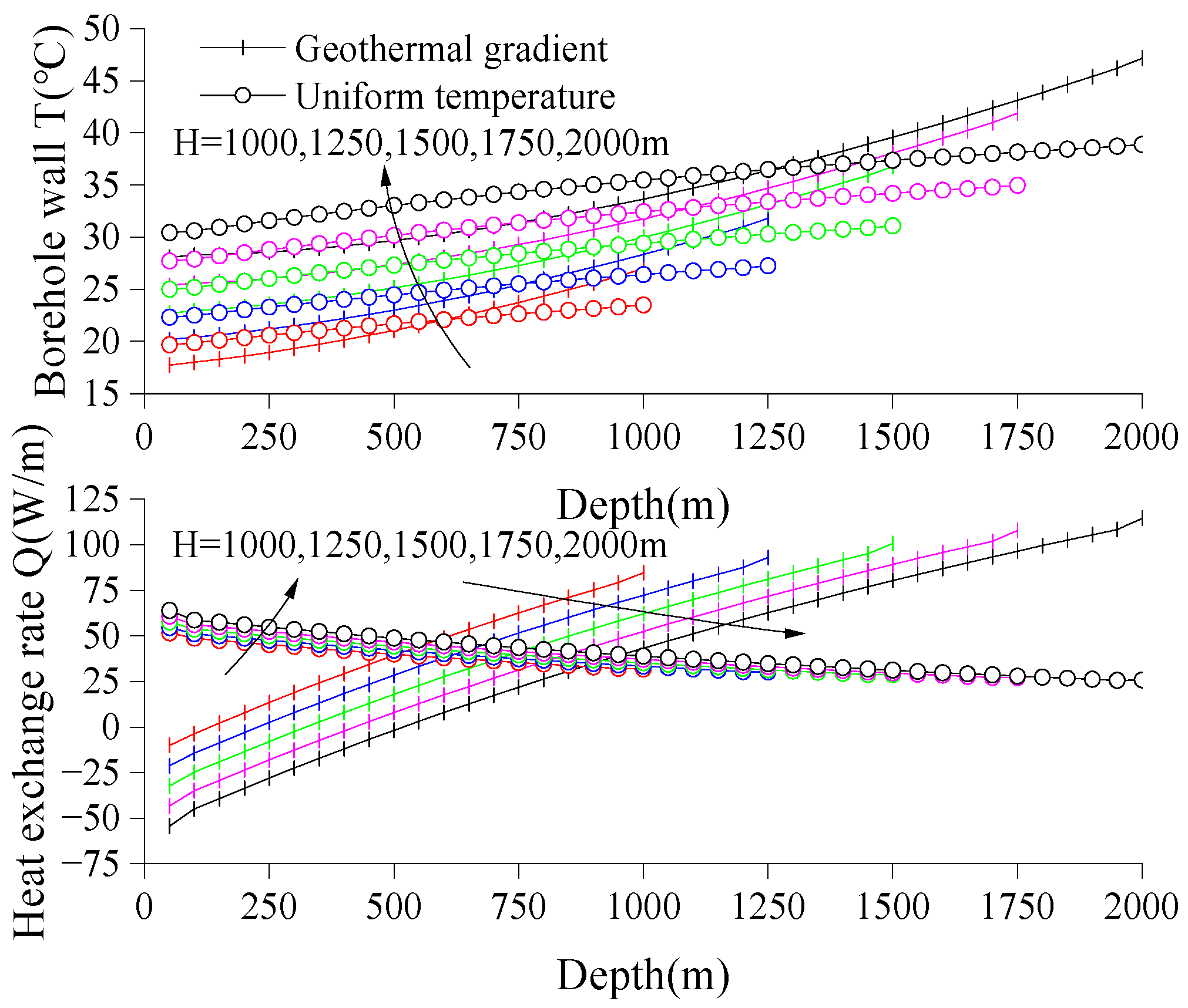
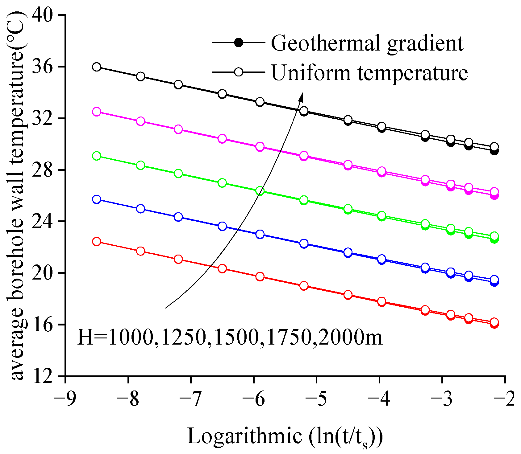
Section 3.1 showed that under the same heat extraction rate for a BHE system, although the axial distribution of borehole wall temperature differs between geothermal gradient and uniform temperature conditions, the average temperature response at the borehole wall is almost identical within the system’s service life. Therefore, the g-function under uniform temperature background can be introduced to calculate the corresponding average temperature response at the borehole wall under geothermal gradient.

For shallow BHEs, g-functions can be conveniently and rapidly retrieved from precomputed g-function databases according to the required system configuration. For heat transfer calculations in medium-deep BHE systems, although no ready-made database exists for direct use, the significant depth (typically above 1500 m) means that axial heat transfer effects manifest later, beyond the practical service life of the BHE. Therefore, the influence of pipe length on heat transfer calculation can be neglected, and the g-function for medium-deep BHEs can be readily calculated using the Infinite Line Source (ILS) model. For g-function calculation of multiple medium-deep BHEs, spatial superposition based on the ILS model can also be used to obtain the g-function for the bore field. The g-function for the ILS model is calculated by Equations (23) and (24) [35].

$$g_{ILS}\left(t,k_s,{\left(\rho c\right)}_s\right)={\displaystyle \frac{1}{4\pi k_s}}{\displaystyle \underset{E}{\overset{\infty }{\int }}\frac{\exp \left(-\beta \right)}{\beta }d\beta }$$

(23)

$$E={\displaystyle \frac{{\left(\rho c\right)}_s{r}_b^2}{4k_{s}t}}$$

(24)

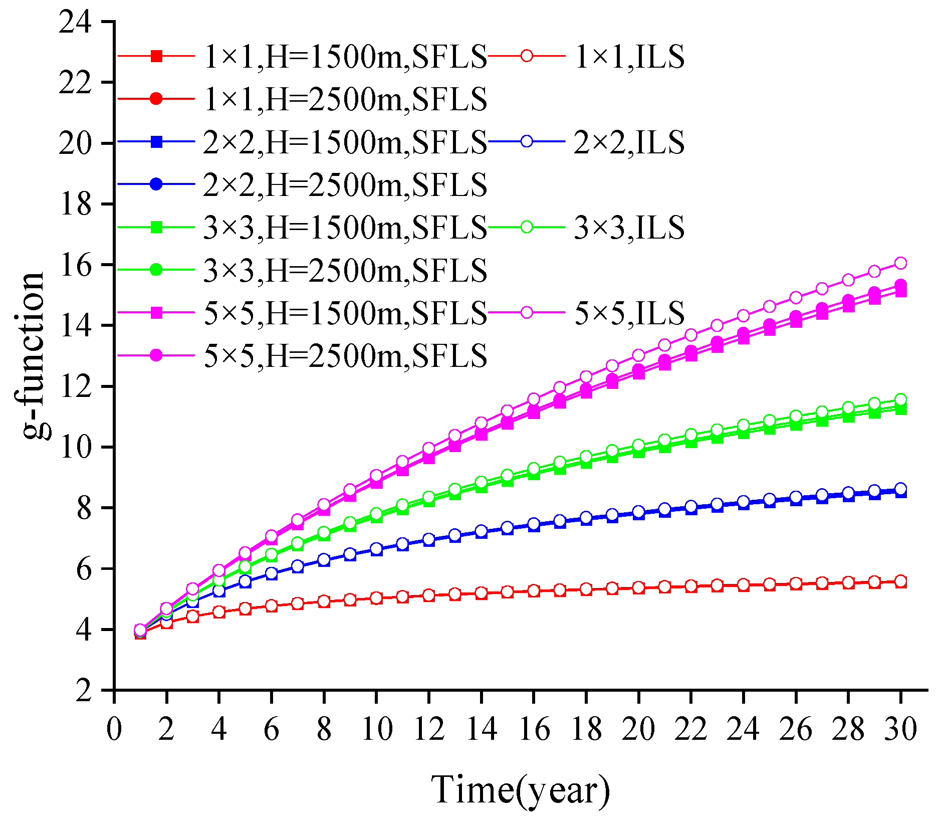
Figure 8 compares the g-functions at the borehole wall calculated by the two models for multiple BHEs with different borehole counts and depths, spaced 15 m apart. The BHE parameters are the same as in Table 3. When the number of boreholes is less than 25, the g-function derived by spatial superposition of the ILS model has a calculation error of less than 6% compared to the SFLS model results over a 30-year period. This calculation error tends to increase with more boreholes, shallower depths, and longer times.

In practical engineering, the spacing between multiple medium-deep BHEs is usually above 15 m, further reducing the influence of inter-borehole interaction on calculations. Additionally, in actual calculations, since the temperature response at the borehole wall is the convolution of the g-function and the corresponding heat exchange rate at each time point, the calculation results at short-to-medium time points mitigate the error at longer time points. Furthermore, the number of boreholes in actual medium-deep BHE installations is typically less than 25, and the operating time is less than 30 years. Therefore, calculating the g-function for multiple medium-deep BHEs using ILS model superposition is effective and meets the needs for the vast majority of multi-bore medium-deep BHE calculations.

4.2.2. Fluid Outlet Correction Temperature Difference $\Delta T_{f,out}$

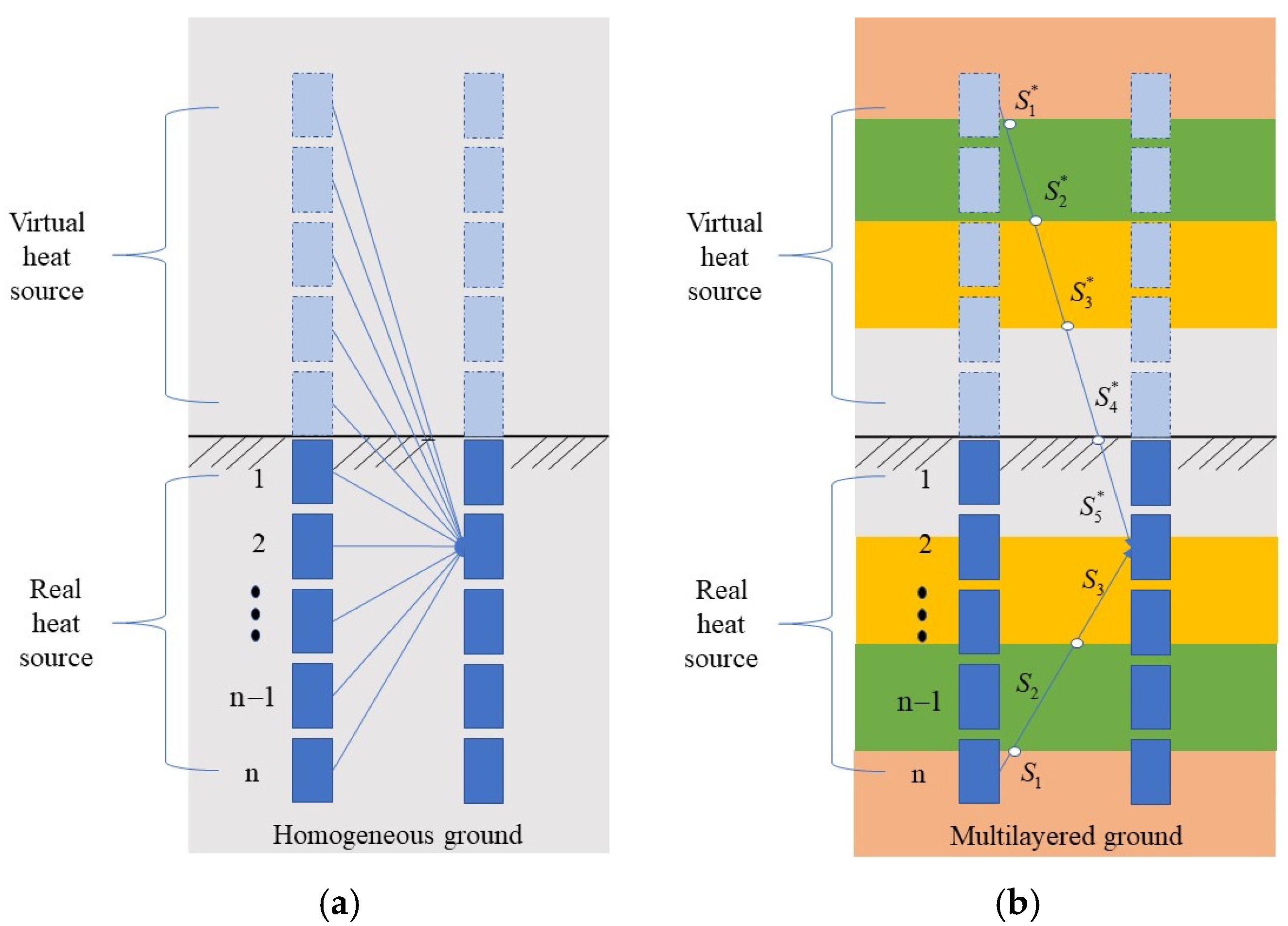
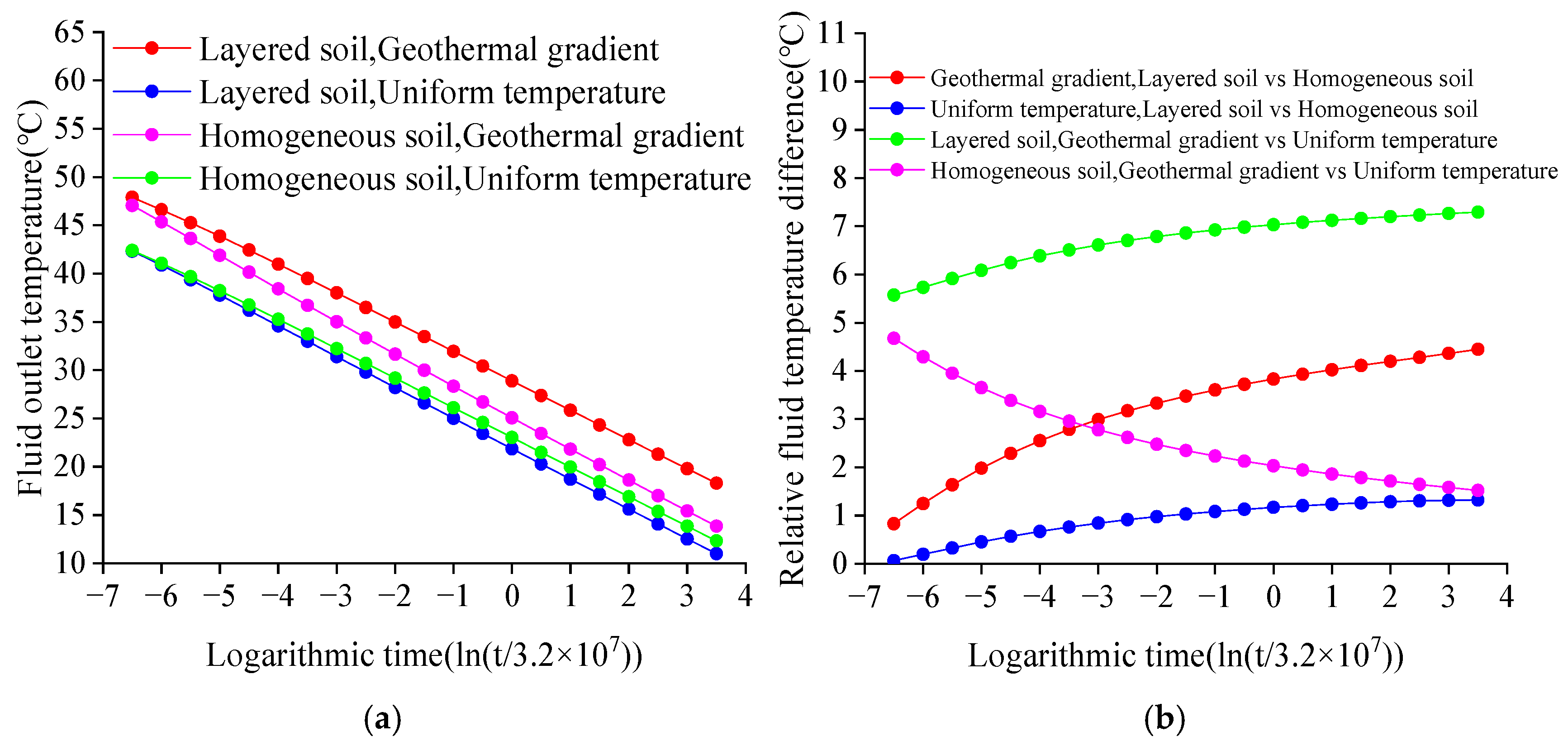
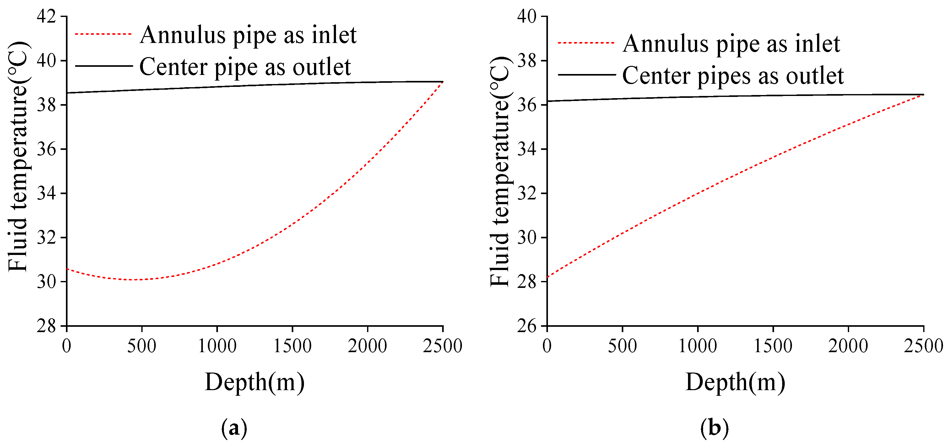
Under the condition of the same heat flux input, although the borehole wall temperature responses under the geothermal gradient and the uniform geothermal temperature are almost the same in the long-term, as can be seen from Section 3, there are significant differences in the fluid outlet temperatures under the two geothermal backgrounds. Figure 9 shows the fluid temperature distribution diagrams under the geothermal gradient and the uniform geothermal temperature under the same heat flux condition. It can be seen that under the geothermal gradient, due to the low temperature of the upper-layer soil and the high temperature of the lower-layer soil, the heat transfer of the fluid in the ground heat exchanger is non-uniform along the depth. The temperature distribution of the downward—flowing fluid in the annulus tube shows a non-linear distribution characteristic, which is related to the longitudinal heat exchange amount of the system. The smaller the heat exchange amount, the more obvious this non-linear distribution characteristic is [36]. For the heat transfer of the ground heat exchanger under the uniform geothermal temperature, because the soil temperature is uniform along the depth, the fluid heat transfer is relatively uniform along the depth, and the fluid temperature distribution is approximately linear compared with that under the geothermal gradient. Under the two geothermal conditions, when the total heat exchange amount of the system is the same, although the average wall temperature at the borehole wall is the same, due to the differences in the fluid temperature distribution, there are significant differences in the final fluid inlet and outlet temperatures.

Figure 9a shows the case of a uniform geothermal temperature with a heat exchange rate per unit length of 80 W/m; Figure 9b shows the case of a geothermal gradient with a heat exchange rate per unit length of 80 W/m.

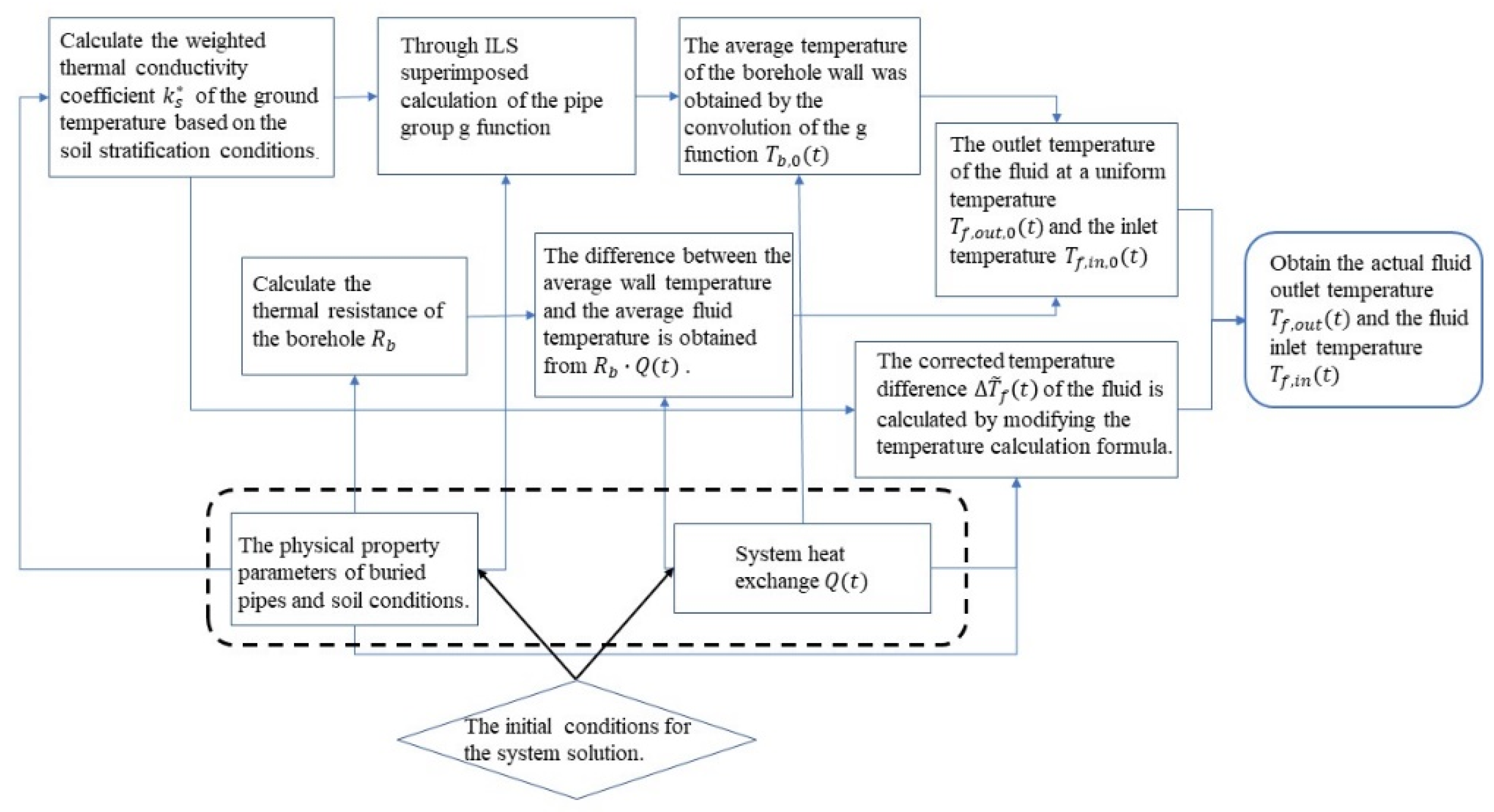
For calculating shallow BHE fluid outlet temperature, a common method is to first obtain the average borehole wall temperature using the g-function, then estimate the average fluid temperature using borehole thermal resistance $R_b$ and total heat exchange Q. The inlet-outlet temperature difference is calculated using flow rate M and fluid specific heat $c_p$. Finally, the inlet and outlet temperatures are derived from the average fluid temperature and the temperature difference, as shown in Equations (25) and (26), where ${\overline{T}}_s$ is the initial average soil temperature and $k_s$ is the soil thermal conductivity.

$$T_{f,out,0}={\overline{T}}_s-{\displaystyle \frac{g\cdot Q}{2\pi k_s}}-R_b\cdot Q+{\displaystyle \frac{Q}{2M{c}_p}}$$

(25)

$$T_{f,in,0}={\overline{T}}_s-{\displaystyle \frac{g\cdot Q}{2\pi k_s}}-R_b\cdot Q-{\displaystyle \frac{Q}{2M{c}_p}}$$

(26)

This estimation method is considered relatively accurate in homogeneous media under uniform soil temperature. However, this approach relies on three conditions:

(1) The fluid heat transfer in the borehole reaches a steady state;

(2) There is no obvious heat short—circuit phenomenon between the upward—flowing and downward—flowing fluids in the ground heat exchanger;

(3) The temperature distribution of the fluid exchanging heat with the soil along the depth should be approximately linear.

Since this estimation method can accurately estimate the fluid outlet temperature under the uniform geothermal temperature, as long as the temperature difference between the fluid outlet temperatures under the geothermal gradient and the uniform geothermal temperature can be given on this basis, the fluid outlet temperature under the geothermal gradient can be calculated by adding this temperature difference to the fluid outlet temperature under the uniform geothermal temperature.

The mathematical expression of this temperature difference can be given by the segmented finite line source model:

$$\begin{array}{cc}\hfill \Delta T_{f,out}\left(t_k\right)& =T_{f,out,gd}\left(t_k\right)-T_{f,out,0}\left(t_k\right)\hfill \\ & ={\displaystyle \frac{1}{\left(f_3\left(1\right)-2f_2\left(1\right)-f_1\left(1\right)\right)}}\\ & {\displaystyle \sum _{v=1}^{n_q}\left[\left(X_3\left(\frac{n_q-v+1}{n_q}\right)-X_3\left(\frac{n_q-v}{n_q}\right)\right)\cdot \left(T_{b,v,gd}\left(t_k\right)-T_{b,v,0}\left(t_k\right)\right)\right]}\end{array}$$

(27)

where $T_{f,out,gd}$ is the fluid outlet temperature under the geothermal gradient, $T_{f,out,0}$ is the fluid outlet temperature under the uniform geothermal temperature, $T_{b,v,gd}$ is the borehole wall temperature of the $v$-th segment of the ground heat exchanger under the geothermal gradient, and $T_{b,v,0}$ is the borehole wall temperature of the v-th segment of the ground heat exchanger under the uniform geothermal temperature.

In the above formula, the mathematical representation and solution of $T_{b,v,gd}\left(t_k\right)-T_{b,v,0}\left(t_k\right)$ are complex and need to be solved by solving the equations outside the borehole simultaneously. However, $T_{b,v,gd}\left(t_k\right)-T_{b,v,0}\left(t_k\right)$ represents the difference in the borehole wall temperature of each segment of the ground heat exchanger under the geothermal gradient and the uniform geothermal temperature. This difference is obviously caused by the difference in the initial geothermal temperatures at different depths under the two geothermal temperature backgrounds and decays continuously with the operation time. Therefore, the difference in the initial geothermal temperatures of each segment under the geothermal gradient and the uniform geothermal temperature, multiplied by an undetermined coefficient $X_s$, is used to replace this part in the formula, and a simplified correction temperature calculation formula is proposed:

$$\begin{array}{cc}\hfill \Delta T_{f,out}\left(t_k\right)=& {\displaystyle \frac{X_s\cdot g_d}{\left(f_3\left(1\right)-2f_2\left(1\right)-f_1\left(1\right)\right)}}\hfill \\ & {\displaystyle \sum _{v=1}^{n_q}\left[\left(X_3\left(\frac{n_q-v+1}{n_q}\right)-X_3\left(\frac{n_q-v}{n_q}\right)\right)\cdot \frac{v-0.5-n_q/2}{n_q}\right]}\end{array}$$

(28)

The coefficient $X_s$ essentially replaces the influencing factors other than the geothermal gradient and the physical parameters inside the borehole that affect the difference in the borehole wall temperature between the geothermal gradient and the uniform geothermal temperature, such as time, buried depth, flow rate, heat exchange amount, thermal conductivity of the backfill material, and thermal conductivity of the soil. Therefore, the influence of these five parameters on the magnitude of the coefficient $X_s$ is approximately expressed by fitting, and then reflected in the calculation of the correction temperature. That is, the correction coefficient $X_s$ should have the following expression:

$$X_s=f\left(t,H,m,Q,k_b,k_s\right)$$

(29)

To determine the expression of $X_s$, a large number of fluid outlet temperatures $T_{f,out,gd}$ under the geothermal gradient and $T_{f,out,0}$ under the uniform geothermal temperature for different layout forms are calculated by the segmented finite line source model. Then, the accurate value of $X_s$ is calculated by the following formula:

$$X_s={\displaystyle \frac{\left(T_{f,out,gd}\left(t_k\right)-T_{f,out,0}\left(t_k\right)\right)\cdot \left(f_3\left(1\right)-2f_2\left(1\right)-f_1\left(1\right)\right)}{g_d\cdot \left[\left(X_3\left(\frac{n_q-v+1}{n_q}\right)-X_3\left(\frac{n_q-v}{n_q}\right)\right)\cdot \frac{v-0.5-\frac{n_q}{2}}{n_q}\right]}}$$

(30)

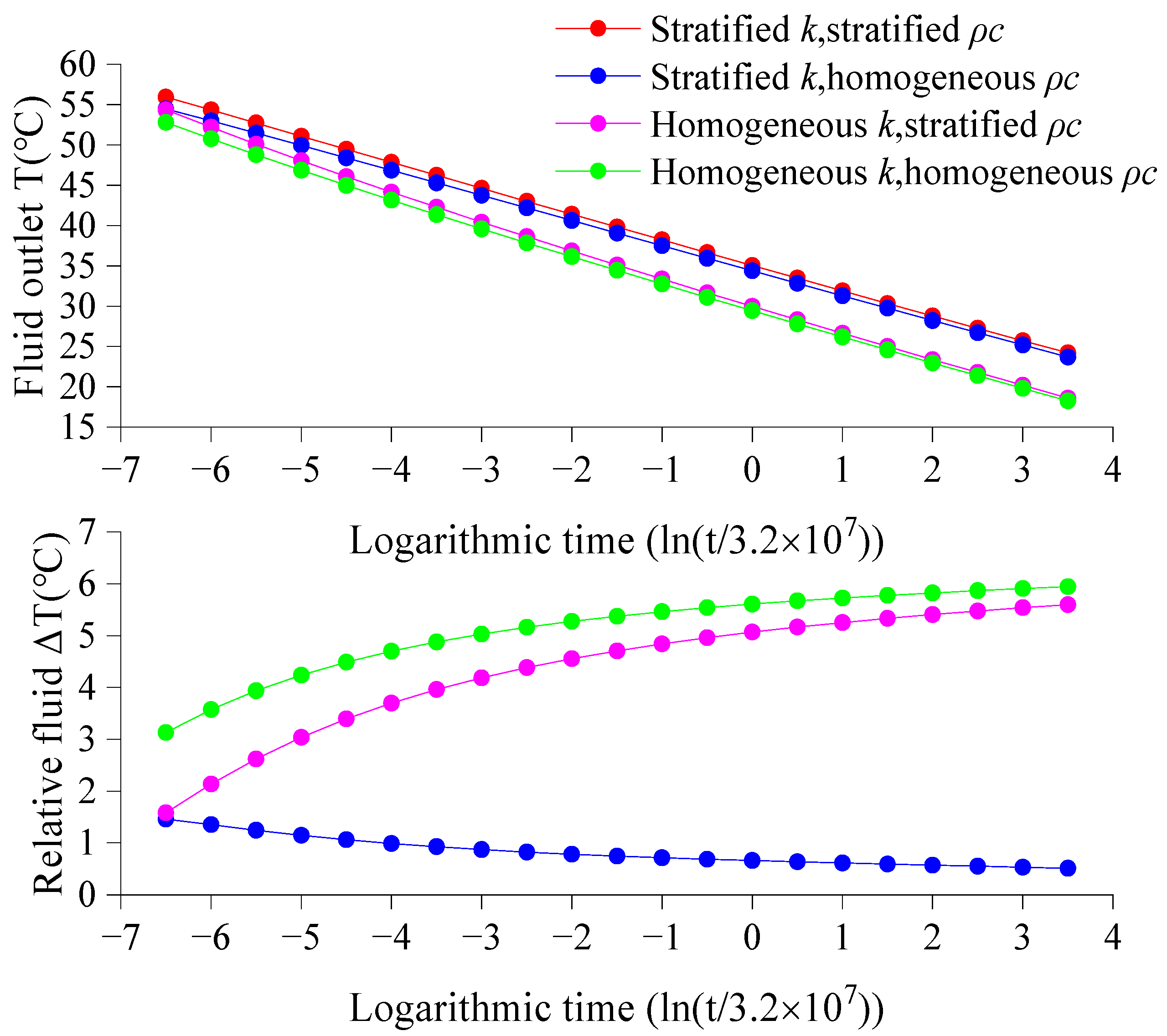
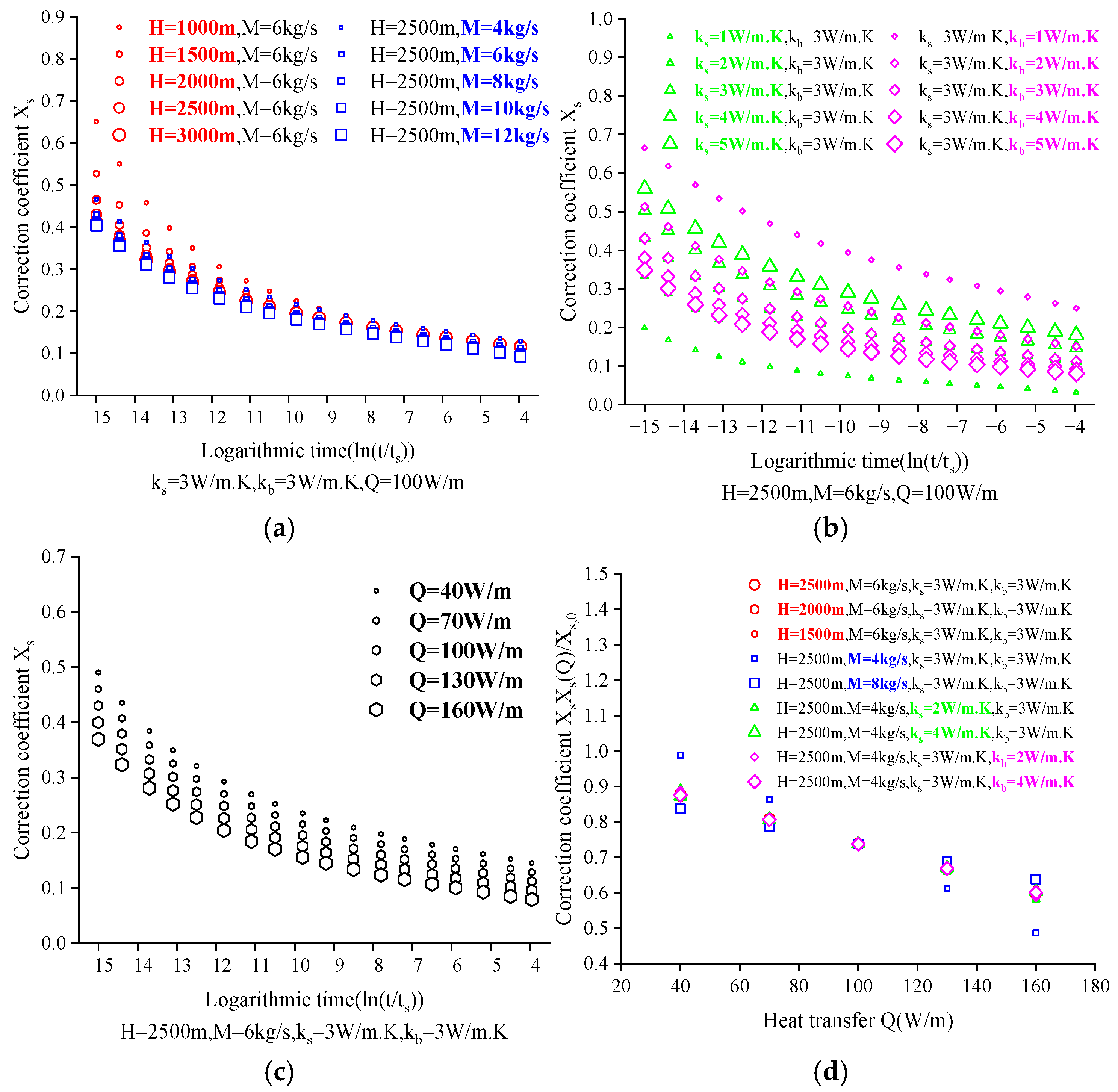
In our assumption, multiple ground heat exchanger parameters affect the determination of the fitted value of $X_s$. It can be seen from Figure 10a–d that the $X_s$ values obtained from different configuration types show a similar trend of change with logarithmic time, forming multiple similar decreasing curves. It can be seen from Figure 10c that at each time point, there is approximately a linear relationship between different heat exchange amounts $Q$ and $X_s$. Figure 10d also reflects the approximate linear relationship between $Q$ and $X_s$ in each configuration. Therefore, the fitting formula of $X_s$ with logarithmic time $\ln ({\displaystyle \frac{t}{t_s}})$ and heat exchange amount $Q$ obtained by the fitting toolbox in MATLAB is as follows:

$$X_s=\left[a\cdot \exp \left(b\cdot \ln \left({\displaystyle \frac{t}{t_s}}\right)\right)+c\cdot \exp \left(d\cdot \ln \left({\displaystyle \frac{t}{t_s}}\right)\right)\right]\cdot \left(-0.002702\cdot Q+1.008\right)$$

(31)

In the above formula, $a$, $b$, $c$, and $d$ are undetermined coefficients, and each coefficient is related to the buried pipe depth $H$, mass flow rate $M$, soil thermal conductivity $k_s$, and backfill material thermal conductivity $k_b$. The specific values of the undetermined coefficients under different configurations are obtained through the fitting tool, as shown in

Table 7. Fitting parameters table.

$\mathit{H}$	$\mathit{M}$	${\mathit{k}}_{\mathit{s}}$	${\mathit{k}}_{\mathit{b}}$	$\mathit{a} \times {10}^5$	b	c	d	${\mathit{X}}_{\mathit{s}}$
1000	6	3	3	2.58	−0.6126	0.0662	−0.1200	0.653
1500	6	3	3	3.38	−0.5756	0.0724	−0.1027	0.528
2000	6	3	3	5.54	−0.5310	0.0768	−0.0921	0.465
2500	6	3	3	8.69	−0.4936	0.0807	−0.0848	0.430
3000	6	3	3	12.78	−0.4632	0.0845	−0.0792	0.410
2500	4	3	3	8.69	−0.4425	0.0946	−0.0764	0.466
2500	6	3	3	8.69	−0.4936	0.0807	−0.0848	0.430
2500	8	3	3	8.69	−0.5391	0.0734	−0.0916	0.416
2500	10	3	3	8.69	−0.5852	0.0685	−0.0977	0.409
2500	12	3	3	8.69	−0.6339	0.0646	−0.1031	0.405
2500	6	1	3	22.11	−0.7857	0.0212	−0.1261	0.199
2500	6	2	3	8.69	−0.5834	0.0510	−0.0985	0.333
2500	6	3	3	3.87	−0.4936	0.0807	−0.0848	0.430
2500	6	4	3	1.73	−0.4345	0.1093	−0.0755	0.503
2500	6	5	3	0.75	−0.3901	0.1366	−0.0684	0.560
2500	6	3	1	0.04	−0.4601	0.1899	−0.0722	0.667
2500	6	3	2	1.74	−0.4682	0.1103	−0.0806	0.514
2500	6	3	3	8.69	−0.4936	0.0807	−0.0848	0.430
2500	6	3	4	24.27	−0.5124	0.0657	−0.0873	0.380
2500	6	3	5	51.42	−0.5261	0.0570	−0.0891	0.348

:

Based on the relationships between the undetermined coefficients $a$, $b$, $c$, $d$ and the parameters of the ground—buried pipes, the method of multiple linear regression fitting was used to determine the correlations among the parameters in the equation, and the fitting expressions for the undetermined coefficients were obtained. Thus, the specific expression of $X_s=f\left(t,H,m,Q,k_b,k_s\right)$ was determined. Finally, the expression for the corrected temperature $\Delta T_{f,out}$ is as follows:

$$\begin{array}{cc}\hfill \Delta T_{f,out}\left(t_k\right)=& {\displaystyle \frac{X_s\cdot g_d}{\left(f_3\left(1\right)-2f_2\left(1\right)-f_1\left(1\right)\right)}}\hfill \\ & {\displaystyle \sum _{v=1}^{n_q}\left[\left(X_3\left(\frac{n_q-v+1}{n_q}\right)-X_3\left(\frac{n_q-v}{n_q}\right)\right)\cdot \frac{v-0.5-\frac{n_q}{2}}{n_q}\right]}\end{array}$$

(32)

$$X_s=\left[a\cdot \exp \left(b\cdot \ln \left({\displaystyle \frac{t}{t_s}}\right)\right)+c\cdot \exp \left(d\cdot \ln \left({\displaystyle \frac{t}{t_s}}\right)\right)\right]\cdot \left(-0.002702\cdot Q+1.008\right)$$

(33)

$$\begin{array}{cc}\hfill a& =2.16\times {10}^{-11}{H}^2-3.51\times {10}^{-8}H+0.18\exp \left(-2.20M\right)+0.0009654\exp \left(-0.40M\right)\hfill \\ & +5.26\times {10}^{-6}{k_s}^3-4.81\times {10}^{-6}{k_s}^2-5.77\times {10}^{-6}{k}_s-0.00012864\end{array}$$

(34)

$$\begin{array}{cc}\hfill b& =7.6\times {10}^{-5}H-0.02372M-0.7392\exp \left(-1.336k_s\right)\hfill \\ & -0.6568\exp \left(-0.1048k_s\right)-0.04863\end{array}$$

(35)

$$\begin{array}{cc}\hfill c& =8.946\times {10}^{-6}H+0.0289k_s+0.329\exp \left(-1.205k_b\right)\hfill \\ & +0.1032\exp \left(-0.122k_b\right)-0.10884\end{array}$$

(36)

$$\begin{array}{cc}\hfill d& =-0.1019\exp \left(-0.00143H\right)-0.106\exp \left(-0.000103H\right)\hfill \\ & -0.08625\exp \left(-1.144k_s\right)-0.1082\exp \left(-0.09278k_s\right)\\ & -0.08304\exp \left(0.01502k_b\right)+0.02905\exp \left(-0.8761k_b\right)+0.16951\end{array}$$

(37)

$$f_1\left(1\right)=\exp \left({\beta }^{\prime }\right)\left[\cosh \left({\gamma }^{\prime }\right)-\delta \sinh \left({\gamma }^{\prime }\right)\right]$$

(38)

$$f_2\left(1\right)=\exp \left({\beta }^{\prime }\right){\displaystyle \frac{{\beta }_{12}^{’}}{{\gamma }^{\prime }}}\sinh \left({\gamma }^{\prime }\right)$$

(39)

$$f_3\left(1\right)=\exp \left({\beta }^{\prime }\right)\left[\cosh \left({\gamma }^{\prime }\right)+\delta \sinh \left({\gamma }^{\prime }\right)\right]$$

(40)

$$X_3\left({\displaystyle \frac{u}{n_q}}\right)=\exp \left({\beta }^{\prime }{\displaystyle \frac{u}{n_q}}\right){\displaystyle \frac{{\beta }_1^{\prime }+{\beta }_2^{\prime }}{{\gamma }^{\prime }}}\sinh \left({\gamma }^{\prime }{\displaystyle \frac{u}{n_q}}\right)$$

(41)

${\beta }_1^{\prime }={\displaystyle \frac{\xi H}{M{c}_p{R}_b}}$, ${\beta }_2^{\prime }={\displaystyle \frac{\left(1-\xi \right)H}{M{c}_p{R}_b}}$, ${\beta }_{12}^{\prime }={\displaystyle \frac{H}{M{c}_p{R}_{12}}}$ are the dimensionless thermal conductivities of the borehole, ${\beta }^{\prime }={\displaystyle \frac{{{\beta }^{\prime }}_2-{{\beta }^{\prime }}_1}{2}}$, ${\gamma }^{\prime }=\sqrt{{\left({{\beta }^{\prime }}_1+{{\beta }^{\prime }}_2\right)}^2/4+{{\beta }^{\prime }}_{12}\left({{\beta }^{\prime }}_1+{{\beta }^{\prime }}_2\right)}$, $\delta ={\displaystyle \frac{1}{{\gamma }^{\prime }}}\left({{\beta }^{\prime }}_{12}+{\displaystyle \frac{{{\beta }^{\prime }}_1+{{\beta }^{\prime }}_2}{2}}\right)$, $R_b$ is the thermal resistance between the water in the annulus tube and the borehole wall, $R_{12}$ is the short—circuit thermal resistance between the fluids in the central tube and the annulus tube, t is the time, $t_s={\displaystyle \frac{H^2}{9{\alpha }_s}}$, ${\alpha }_s$ is the soil thermal diffusivity, $M$ is the mass flow rate, $c_p$ is the specific heat of the fluid, the number of segments $n_q=20$, $k_b$ is the thermal conductivity of the backfill material, $k_s$ is the thermal conductivity of the soil, Q is the heat exchange rate per unit length.

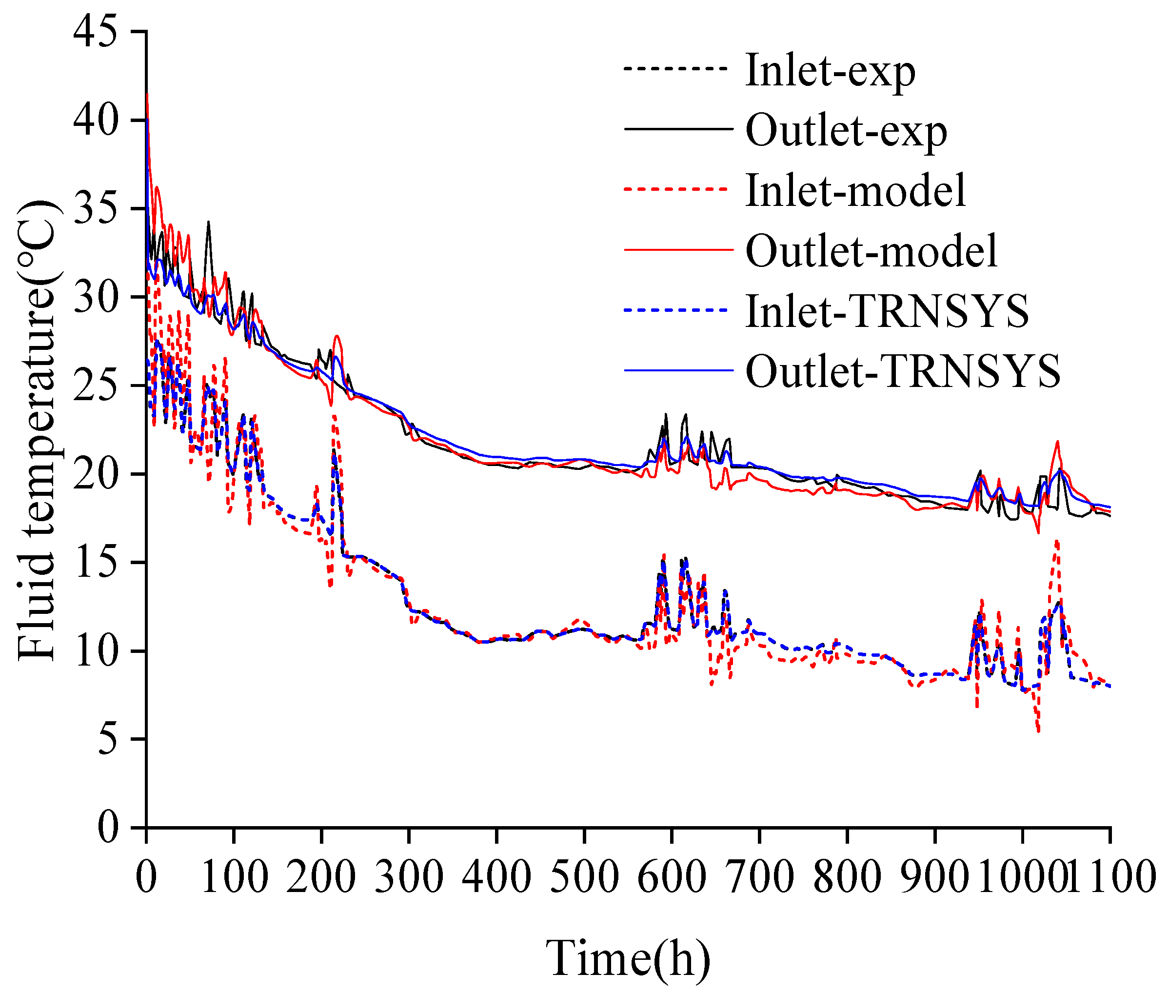
4.2.3. Error Comparison of Fluid Temperature Correction Method

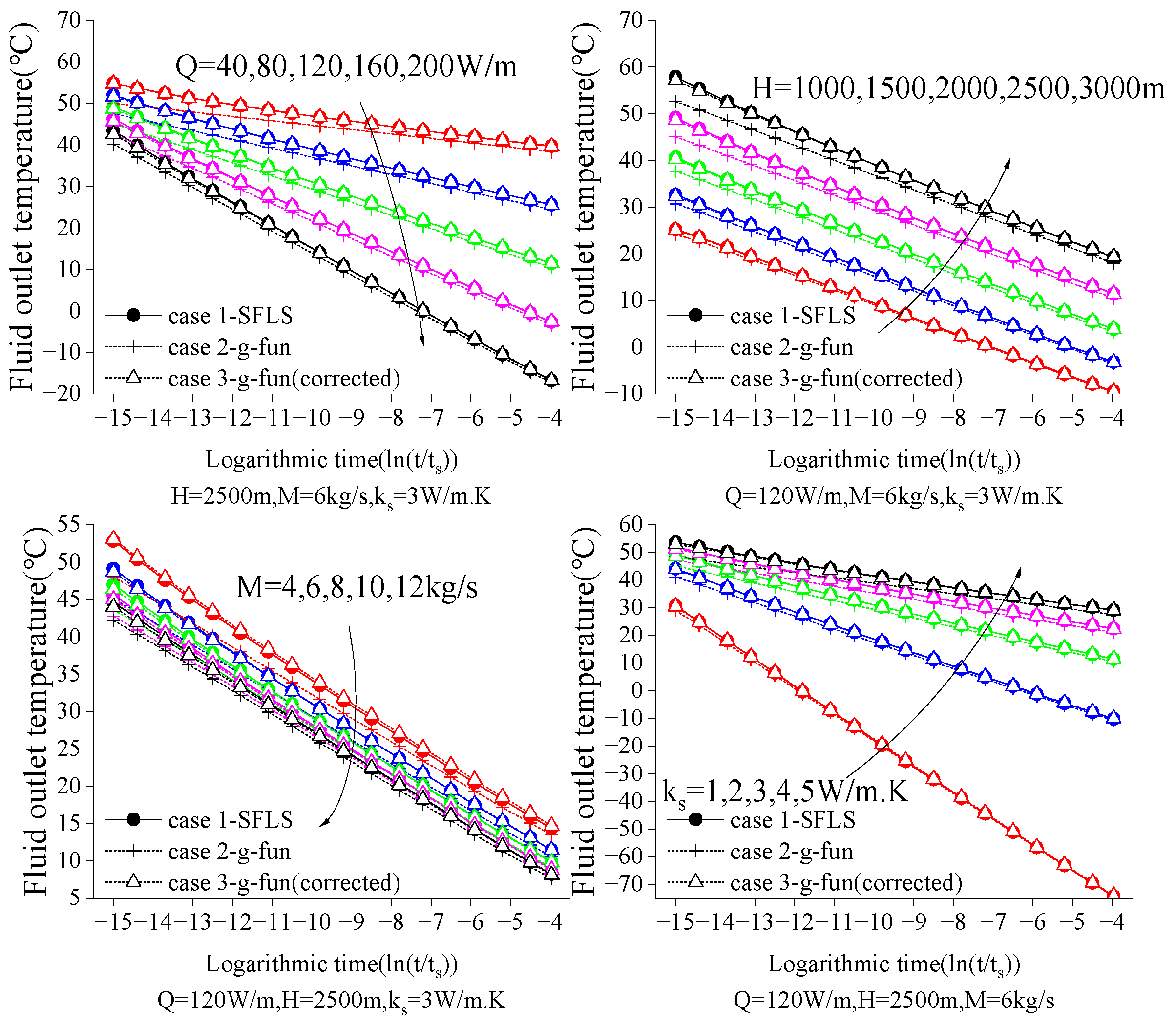
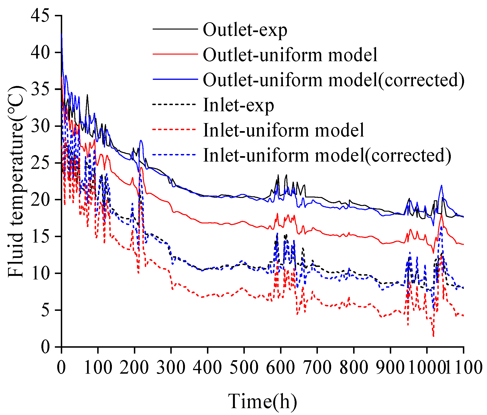
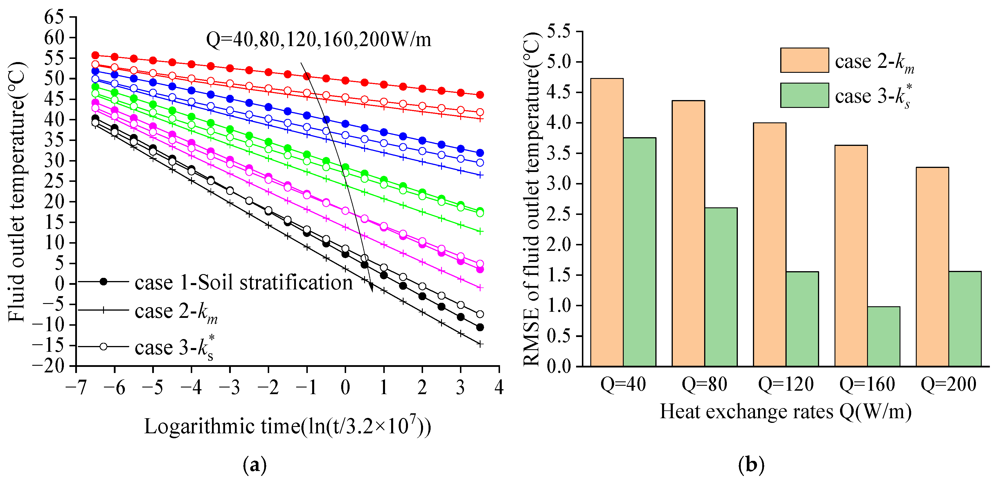
The physical parameter configuration for a single-borehole BHE is as in Table 3, the geothermal gradient is 0.03 °C/m, and the surface temperature is 15 °C. We compare the relative error between the fluid outlet temperature calculated using the g-function (derived from ILS) before and after applying the fluid temperature correction method, and the fluid outlet temperature calculated using the SFLS model. The three calculation cases are shown in

Table 8. Three Calculation Cases.

	Calculation Method	$\mathbf{Fluid}\mathbf{Outlet}\mathbf{Temperature}{\mathit{T}}_{\mathit{f},\mathit{o}\mathit{u}\mathit{t}}$
Case 1	SFLS Analytical Solution	$T_{f,out,gd}$ solved by Equations (28)–(30)
Case 2	g-function	$T_{f,out,0}={\overline{T}}_s-{\displaystyle \frac{g_{ILS}\cdot Q}{2\pi k_s}}-R_b\cdot Q+{\displaystyle \frac{Q}{2M{c}_p}}$
Case 3	g-function + Fluid Correction Temperature	${\tilde{T}}_{f,out,gd}={\overline{T}}_s-{\displaystyle \frac{g_{ILS}\cdot Q}{2\pi k_s}}-R_b\cdot Q+{\displaystyle \frac{Q}{2M{c}_p}}+\Delta {\tilde{T}}_{f,out}$

. Case 1 is the analytical solution calculated by the SFLS model under geothermal gradient and serves as the standard reference for Cases 2 and 3. Case 2 is the g-function estimated fluid temperature result. Case 3 adds the fluid correction temperature difference to the calculation result of Case 2. Here, ${\overline{T}}_s$ is the average soil temperature, $R_b$ is the borehole thermal resistance, $k_s$ is the soil thermal conductivity, Q is the heat exchange rate per meter, and M is the BHE flow rate.

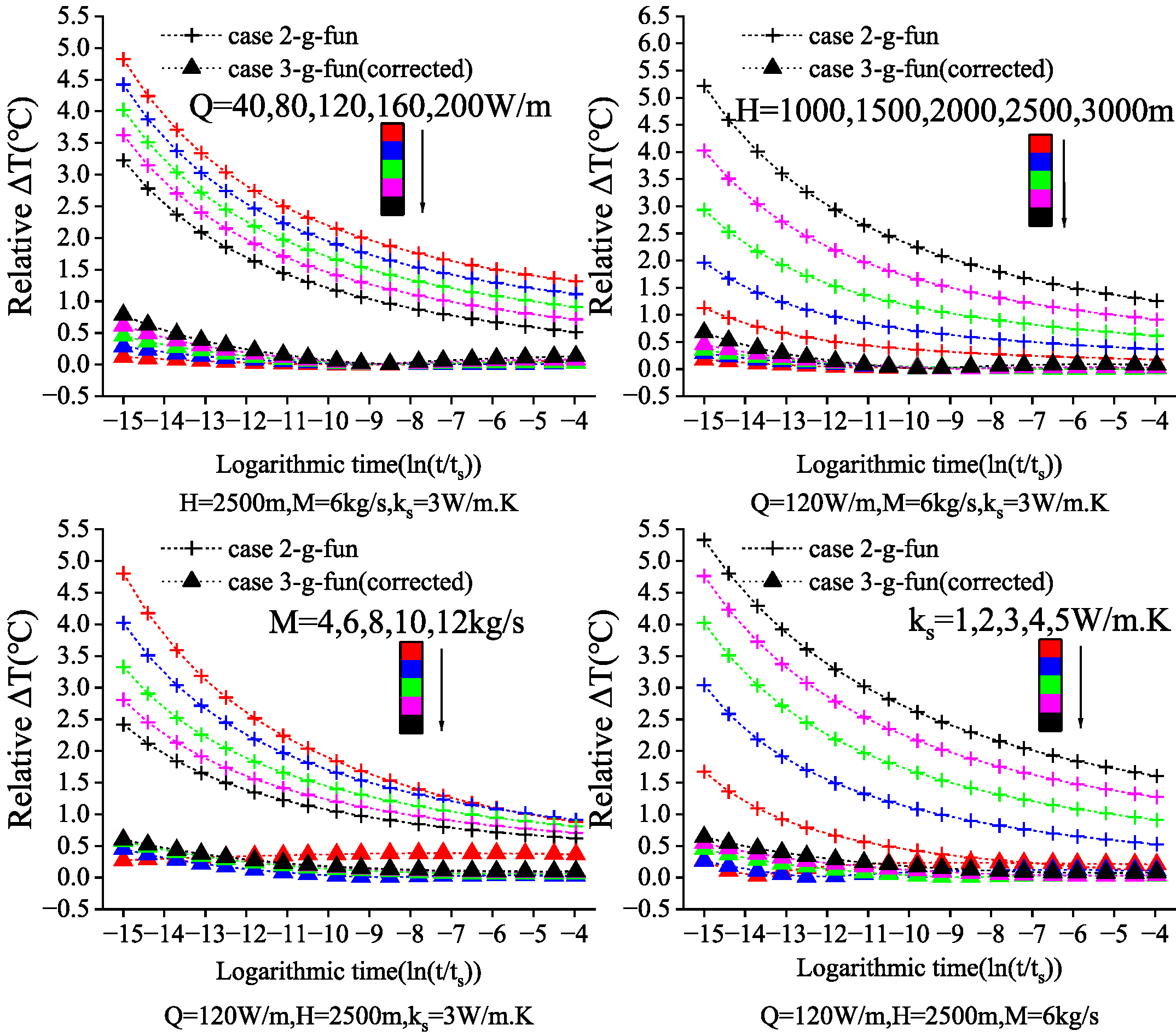
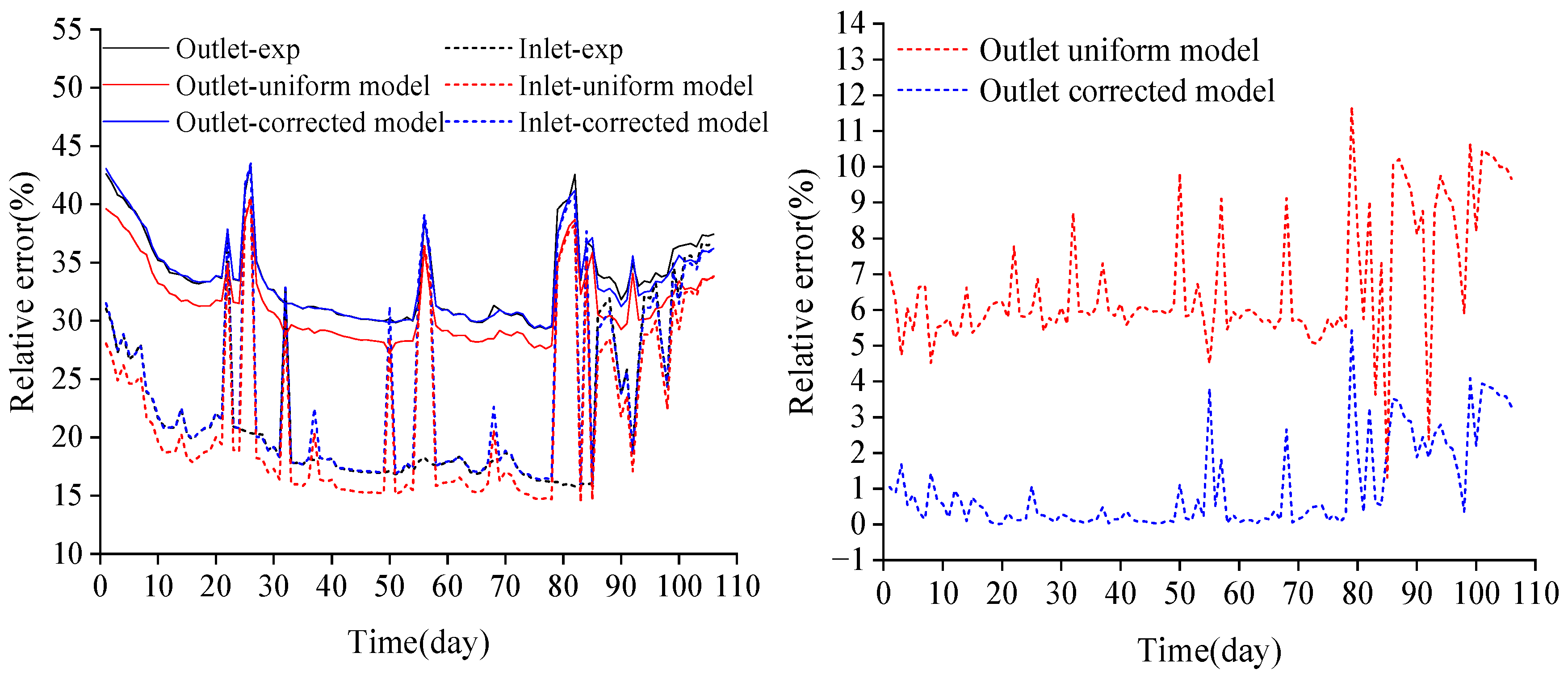
Using the heat exchange rate per meter Q, borehole depth H, BHE flow rate M, and soil thermal conductivity $k_s$ as key influencing parameters for the simplified algorithm, a single-variable control method is employed. Other parameters are fixed while observing the impact of the target parameter on the algorithm’s outlet temperature error. Figure 11 and Figure 12 respectively represent the relative error in fluid outlet temperature between Cases 2, 3 and Case 1, under heat extraction rates from 40 to 200 W/m, depths from 1000 to 3000 m, flow rates from 4 to 12 kg/s, and soil thermal conductivities from 1 to 5 W/m·K.

Figure 12 shows that the fluid temperature calculation errors for Cases 2 and 3 relate to Case 1 gradually decrease over time. The fitting error of the fluid correction temperature difference method (Case 3) is significantly affected by physical parameters almost exclusively during the initial operation of the BHE system. Specifically, the initial fitting error increases relatively under high heat extraction rates, deeper borehole depths, and higher soil thermal conductivity, but still maintains high accuracy. The average fluid error of the corrected temperature difference method (Case 3) compared to the SFLS analytical solution (Case 1) is less than 0.4 °C across all the fitted parameter ranges. Furthermore, Figure 12 shows that the calculation error of the corrected fluid outlet temperature in Case 3 is significantly reduced compared to the uncorrected calculation error in Case 2, with an error reduction rate exceeding 80%.

4.3. Example Verification of the Simplified Calculation Method

The simplified algorithm integrates the simplifications of soil stratification and geothermal gradient. Figure 13 shows the simplified algorithm. It is necessary to verify the effectiveness of the comprehensive simplified algorithm through cases. The geothermal gradient is the main influencing factor in the heat transfer calculation of deep—hole ground heat exchangers, so more attention should be paid to the effectiveness of its simplification. In this study, two cases were used to verify the simplified algorithm.

(1) Example 1: Using the same example data as in the verification of the analytical solution above, comprehensively verify the effectiveness of the simplified algorithm in calculating the fluid temperature response of medium—deep multi-borehole ground heat exchangers under the background of soil layering and geothermal gradient.

(2) Example 2: Comparing with the operation data of another actual project in Xi’an, the soil in this ground—source heat pump system is regarded as uniformly distributed, and only the geothermal gradient background is considered. The depth of the ground heat exchanger is deeper than that in Example 1, which is used to further verify the effectiveness of the simplified algorithm in calculating the fluid temperature response of the ground heat exchanger under the geothermal gradient.

4.3.1. Example Verification 1

To verify the effectiveness of the above—mentioned modified and simplified algorithm, the actual operation data of Xi’an used to verify the analytical model above is also used for comparison. The operation parameters are shown in the above Table 1 and Table 2 and the comparison results of the algorithms are shown in Figure 14. In the uniform model, the soil layering is replaced by the average thermal conductivity, and the geothermal gradient is replaced by a uniform geothermal temperature. The fluid temperature response is calculated by the g-function of the pipe group generated by the superposition of the ILS model. In the uniform model (modified), the soil layering is replaced by the geothermal—gradient—weighted thermal conductivity, and the geothermal gradient is replaced by a uniform geothermal temperature and a corrected fluid temperature difference. After calculating the temperature response by the g-function of the pipe group generated by the superposition of the ILS model, the final fluid temperature response is obtained by adding the corrected fluid temperature difference.

The RMSE of the outlet fluid temperature of the uniform model is 3.91 °C, while that of the uniform model (modified) under the simplified algorithm is 1.07 °C. The calculation accuracy is greatly improved under the simplified algorithm. At the same time, compared with the calculation time of the analytical solution above, the calculation time of the multi-borehole segmented finite line source model is 119.085 s, while the simplified algorithm does not require complex integral calculations, and the calculation time is only 0.123 s. The calculation speed is increased by approximately 968 times.

4.3.2. Example Verification 2

To further verify the effectiveness of the modified and simplified algorithm under the geothermal gradient, it is compared with the operation data of a deep—hole ground heat exchanger group in a heating season of an actual project in Xi’an. In this project, the soil layer is uniformly distributed, and the layout parameters of the ground heat exchanger are shown in

Table 9. System and model parameters.

Parameter	Value
Depth of Ground Heat Exchanger (m)	2500
Number of Boreholes	8
Buried—Pipe Spacing (m)	18
Outer—Pipe Material	Stainless Steel J55
Outer—Pipe Diameter × Wall Thickness (mm × mm)	178 × 4.5
Outer—Pipe Thermal Conductivity (W/m·K)	54
Outer—Pipe Heat Capacity (kJ/kg·K)	0.47
Outer—Pipe Density (kg/m3)	7820
Inner—Pipe Material	HDPE
Inner—Pipe Diameter × Wall Thickness (mm × mm)	110 × 4.0
Inner—Pipe Thermal Conductivity (W/(m·K))	0.04
Inner—Pipe Heat Capacity (kJ/kg·K)	2.1
Inner—Pipe Density (kg/m3)	930
Borehole Diameter (mm)	400
Thermal Conductivity of Backfill Material (W/m·K)	2.0
Heat Capacity of Backfill Material (kJ/kg·K)	0.85
Density of Backfill Material (kg/m3)	2700
Average Thermal Conductivity of Rock Stratum (W/(m·K))	3
Average Heat Capacity of Rock Stratum (kJ/kg·K)	860
Average Density of Rock Stratum (kg/m3)	2990
Rock—Stratum Surface Temperature (°C)	13.0
Average Temperature Rise Gradient (°C/m)	0.0285

:

The comparison between the actual operation data and the calculation results of the modified and simplified algorithm and those under the uniform geothermal temperature (before modification) is as Figure 15:

In the comparison with the actual operation process, before modification, that is, the RMSE between the calculated outlet water temperature $T_{f,out}$ under the uniform geothermal temperature and the measured outlet water temperature $T_{f,out}$ is 2.375 °C, while the RMSE between the outlet water temperature $T_{f,out}^{*}$ under the modified and simplified algorithm and the measured outlet water temperature $T_{f,out}$ is 0.595 °C. The average relative error of the fluid temperature is reduced from 6.64% before modification to 0.97% after modification, and the calculation relative error rate is reduced by 85%.

For the situation where the error increases after 85 days, it is because within this time range, the heat exchange of the ground heat exchanger in actual operation is significantly reduced, the temperature difference between the inlet and outlet water is small, and most of the time the temperature difference between the inlet and outlet water is less than 1 °C, which deviates from the normal range of heat exchange of medium- and deep-buried ground heat exchangers, that is, it deviates from most of the normal working conditions targeted by the fitting correction. Therefore, the fitting correction effect is relatively reduced, but it is still significantly better than the unmodified result. This indicates that this simplified algorithm is simple and effective, and can conveniently and quickly calculate the temperature response of deep multi-borehole ground heat exchangers under the geothermal gradient condition.

5. Discussion and Analysis

5.1. Coupling Effect of Geothermal Gradient and Stratification

5.1.1. Impact of Geothermal Gradient

The geothermal gradient is the dominant factor influencing the heat transfer calculation for medium-deep BHEs. In deep BHE systems, the geothermal gradient typically ranges from 0.02–0.03 °C/m. This means that over a depth of 2000 m, the temperature difference between the upper and lower soil layers can reach 60 °C. This large temperature difference causes significant variations in the heat exchange capacity of the fluid at different depths, thereby affecting the fluid temperature distribution along the depth.

By comparing heat transfer models under geothermal gradient and uniform temperature, this study found that the fluid temperature distribution under geothermal gradient exhibits a distinct non-linear characteristic, whereas under uniform temperature, it is approximately linear. This non-linear distribution renders traditional uniform temperature models prone to significant errors (exceeding 10%) under geothermal gradient conditions, especially in deep BHE systems. Therefore, modeling heat transfer under geothermal gradient is crucial for accurate calculations in deep BHEs.

5.1.2. Impact of Soil Stratification

The influence of soil stratification on heat transfer calculation depends on the presence of the geothermal gradient. Under geothermal gradient conditions, the impact of soil stratification is more pronounced. By comparing stratified soil models with homogeneous soil models, this study found that stratified soil exhibits stronger heat exchange capacity in deep BHE systems, particularly due to the combined effect of high thermal conductivity layers and high temperatures in deeper zones. For instance, at a depth of 2500 m, the outlet fluid temperature in stratified soil was 3.18 °C higher than in homogeneous soil under geothermal gradient, whereas under uniform temperature, it was only 0.91 °C higher.

Furthermore, the variance in thermal conductivity differences between soil layers significantly affects heat transfer calculation. When the differences in thermal conductivity between layers are large, the discrepancy between the stratified soil heat transfer model and the homogeneous soil model becomes more significant. For BHE heat transfer calculations in stratified soil under geothermal gradient, the soil heat capacity can be simplified using averaging (average temperature calculation error is 0.83 °C), while the layered nature of soil thermal conductivity must be maintained in the model (average temperature calculation error between homogeneous and stratified thermal conductivity is 4.33 °C). Therefore, under geothermal gradient, modeling soil stratification is key to improving the accuracy of heat transfer calculations.

The geothermal gradient amplifies the high thermal conductivity of deep soil, intensifying the non-uniform distribution of heat exchange rate along the depth. The impact of soil stratification is significant only when the gradient is present (average temperature difference reaches 3.18 °C). This conclusion provides a theoretical basis for sensitivity analysis of geological parameters.

5.2. Model Advantages and Limitations

5.2.1. Multi-Bore Segmented Finite Line Source Analytical Model

Traditional numerical models often require complex meshing and iterative calculations, leading to longer computation times. Compared to traditional numerical models, the multi-bore SFLS analytical model proposed in this paper significantly reduces computational complexity by combining the composite medium method and Green’s function. Moreover, this analytical model better reflects the heat exchange process between the BHE and the soil, especially under geothermal gradient and stratified conditions, accurately capturing the non-linear fluid temperature distribution along the depth. However, under multi-bore, multi-segment scenarios, computational load increases exponentially, and time consumption remains an issue.

5.2.2. Simplified Algorithm

The proposed simplified algorithm transforms complex geological heat transfer problems into simple problems based on homogeneous soil and uniform temperature, followed by correction. It significantly reduces calculation time with almost no sacrifice in accuracy. Using Engineering Case 1 as context, calculating the temperature response over one heating season took 119.085 s with the multi-bore SFLS model, but only 0.123 s with the simplified algorithm—an efficiency improvement of approximately 968 times. The fluid temperature RMSE between the multi-bore SFLS model and actual data was 1.02 °C, while for the simplified algorithm, it was 1.07 °C. Validation with actual engineering data showed high agreement (RMSE < 1.1 °C) between the simplified algorithm’s simulation results and measured data, proving its applicability under complex geological conditions. It is suitable for long-term dynamic simulation.

Compared to uncorrected homogeneous models, the simplified algorithm greatly improves calculation accuracy under complex soil backgrounds. Validation from Engineering Case 1 showed that under coupled soil stratification and geothermal gradient, the fluid temperature RMSE between the homogeneous model and actual data was 3.91 °C. With the correction algorithm, this RMSE reduced to 1.07 °C. Validation from Engineering Case 2 showed that under homogeneous soil considering only geothermal gradient, the correction algorithm reduced the outlet temperature RMSE from 2.375 °C to 0.589 °C (0.595 °C in Figure 4, Figure 5, Figure 6, Figure 7, Figure 8, Figure 9, Figure 10, Figure 11 and Figure 12), and the average relative error of fluid temperature decreased from 6.64% to 0.97%. Accuracy is significantly improved. Furthermore, within the conventional heat extraction range (80–120 W/m), the error of the simplified algorithm is <5%, meeting engineering accuracy requirements.

5.2.3. Limitations

Although the simplified algorithm performs well under most conditions, it has some limitations. The geothermal-weighted thermal conductivity method shows larger errors (RMSE 3.75 °C) under low heat extraction conditions (<40 W/m). This is because, at low heat extraction rates, the fluid temperature is close to the soil temperature. The lower thermal conductivity of shallow soil causes the fluid to release heat to the soil, while the higher thermal conductivity of deep soil enhances the fluid’s ability to extract heat from deep soil. This non-uniform heat exchange distribution makes the homogeneous thermal conductivity approximation less accurate under low heat extraction rates. For low heat transfer conditions, the computed geothermal-weighted thermal conductivity can be proportionally scaled up based on its relative magnitude to conventional extraction loads to mitigate this error.

6. Conclusions

This study addressed the heat transfer problem of medium-deep borehole heat exchangers (BHEs) under soil stratification and geothermal gradient. An analytical model was developed, and a simplified algorithm was proposed. Key conclusions are:

1. Analytical Model Development: A multi-borehole Segmented Finite Line Source (SFLS) model was established. Soil stratification was handled using the composite medium method, and geothermal gradient effects were incorporated via the superposition principle. This model accurately reflects the non-linear fluid temperature distribution along the borehole depth, providing a theoretical basis for analyzing coupled geological effects.

2. Innovative Simplified Algorithm: Two key simplification methods were introduced:

(1) Geothermally-Weighted Thermal Conductivity Method: The equivalent homogeneous thermal conductivity for stratified soil is calculated by weighting layer conductivities $k_s^{*}={\displaystyle \frac{{\displaystyle \sum _{i=1}^n{k}_{s,i}\cdot T_{s,i}}\cdot h_i}{T_s\cdot H}}$ with their geothermal temperature and thickness. Within the conventional heat extraction range (80–120 W/m), this reduced the fluid outlet temperature Root Mean Square Error (RMSE) from 3.81 °C (traditional averaging) to 1.67 °C.

(2) Fluid Temperature Correction Difference Method: The fluid temperature under geothermal gradient is rapidly calculated by combining the g-function (for uniform temperature) with a fitted correction term. This method reduced outlet temperature errors by over 80%, achieving an RMSE below 1.1 °C against measured data.

3. Validation with Engineering Projects: Data from two projects in Xi’an confirmed effectiveness:

(1) Compared to the SFLS model (Case 1: stratified soil + gradient), the simplified algorithm reduced computation time by ~968 times (0.123 s vs. 119.085 s) while maintaining comparable accuracy (fluid temp RMSE: 1.07 °C vs. 1.02 °C).

(2) Compared to uncorrected homogeneous models, the algorithm significantly improved accuracy: In Case 1, RMSE dropped from 3.91 °C to 1.07 °C. In Case 2 (homogeneous soil + gradient), RMSE dropped from 2.375 °C to 0.595 °C, and the average relative error decreased from 6.64% to 0.97%.

4. Future Work: Extending experimental validation to diverse geological conditions (e.g., high-salinity strata, fractured bedrock); Investigating complex borehole layouts (e.g., irregular clusters, multi-depth configurations); Integrating the algorithm with real-time control systems for hybrid renewable energy applications.

References

1. Lake, A.; Rezaie, B.; Beyerlein, S. Review of district heating and cooling systems for a sustainable future. Renew. Sustain. Energy Rev. 2017, 67, 417–425. [Google Scholar] [CrossRef]
2. Zheng, W.; Zhang, Y.; Xia, J.; Jiang, Y. Cleaner heating in Northern China: Potentials and regional balances. Resour. Conserv. Recycl. 2020, 160, 104897. [Google Scholar] [CrossRef]
3. Li, J.; Xu, W.; Li, J.; Huang, S.; Li, Z.; Qiao, B.; Yang, C.; Sun, D.; Zhang, G. Heat extraction model and characteristics of coaxial deep borehole heat exchanger. Renew. Energy 2021, 169, 738–751. [Google Scholar] [CrossRef]
4. Sapinska-Sliwa, A.; Rosen, M.A.; Gonet, A.; Sliwa, T. Deep Borehole Heat Exchangers—A Conceptual and Comparative Review. Int. J. Air-Cond. Refrig. 2016, 24, 1630001. [Google Scholar] [CrossRef]
5. Luo, Y.; Xu, G.; Zhang, S.; Cheng, N.; Tian, Z.; Yu, J. Heat extraction and recover of deep borehole heat exchanger: Negotiating with intermittent operation mode under complex geological conditions. Energy 2022, 241, 122510. [Google Scholar] [CrossRef]
6. Wang, Z.; Wang, F.; Liu, J.; Ma, Z.; Han, E.; Song, M. Field test and numerical investigation on the heat transfer characteristics and optimal design of the heat exchangers of a deep borehole ground source heat pump system. Energy Convers. Manag. 2017, 153, 603–615. [Google Scholar] [CrossRef]
7. Deng, J.; Wei, Q.; Liang, M.; He, S.; Zhang, H. Field test on energy performance of medium-depth geothermal heat pump systems (MD-GHPs). Energy Build. 2019, 184, 289–299. [Google Scholar] [CrossRef]
8. Huang, Y.; Zhang, Y.; Xie, Y.; Zhang, Y.; Gao, X.; Ma, J. Field test and numerical investigation on deep coaxial borehole heat exchanger based on distributed optical fiber temperature sensor. Energy 2020, 210, 118643. [Google Scholar] [CrossRef]
9. Pan, S.; Kong, Y.; Chen, C.; Chai, J. Optimization of Deep Borehole Heat Exchangers Using Genetic Algorithms. Geothermics 2021, 90, 102003. [Google Scholar]
10. Liu, J.; Wang, F.; Gao, Y.; Zhang, Y.; Cai, W.; Wang, M.; Wang, Z. Influencing factors analysis and operation optimization for the long-term performance of medium-deep borehole heat exchanger coupled ground source heat pump system. Energy Build. 2020, 226, 110385. [Google Scholar] [CrossRef]
11. Li, C.; Guan, Y.; Wang, X.; Zhou, C.; Xun, Y.; Gui, L. Experimental and numerical studies on heat transfer characteristics of vertical deep-buried U-bend pipe in intermittent heating mode. Geothermics 2019, 79, 14–25. [Google Scholar] [CrossRef]
12. Song, X.; Wang, G.; Shi, Y.; Li, R.; Xu, Z.; Zheng, R.; Wang, Y.; Li, J. Numerical analysis of heat extraction performance of a deep coaxial borehole heat exchanger geothermal system. Energy 2018, 164, 1298–1310. [Google Scholar] [CrossRef]
13. Song, X.; Zheng, R.; Li, G.; Shi, Y.; Wang, G.; Li, J. Heat extraction performance of a downhole coaxial heat exchanger geothermal system by considering fluid flow in the reservoir. Geothermics 2018, 76, 190–200. [Google Scholar] [CrossRef]
14. Luo, J.; Rohn, J.; Bayer, M.; Priess, A.; Xiang, W. Analysis on performance of borehole heat exchanger in a layered subsurface. Appl. Energy 2014, 123, 55–65. [Google Scholar] [CrossRef]
15. Perego, R.; Guandalini, R.; Fumagalli, L.; Aghib, F.S.; De Biase, L.; Bonomi, T. Sustainability evaluation of a medium scale GSHP system in a layered alluvial setting using 3D modeling suite. Geothermics 2016, 59, 14–26. [Google Scholar] [CrossRef]
16. Florides, G.A.; Christodoulides, P.; Pouloupatis, P. Single and double U-tube ground heat exchangers in multiple-layer substrates. Appl. Energy 2013, 102, 364–373. [Google Scholar] [CrossRef]
17. Karabetoglu, S.; Ozturk, Z.F.; Kaslilar, A.; Juhlin, C.; Sisman, A. Effect of layered geological structures on borehole heat transfer. Geothermics 2021, 91, 102043. [Google Scholar] [CrossRef]
18. Fang, L.; Diao, N.; Shao, Z.; Zhu, K.; Fang, Z. A computationally efficient numerical model for heat transfer simulation of deep borehole heat exchangers. Energy Build. 2018, 167, 79–88. [Google Scholar] [CrossRef]
19. Liu, J.; Wang, F.; Cai, W.; Wang, Z.; Li, C. Numerical investigation on the effects of geological parameters and layered subsurface on the thermal performance of medium-deep borehole heat exchanger. Renew. Energy 2020, 149, 384–399. [Google Scholar] [CrossRef]
20. Beier, R.A.; Fossa, M.; Morchio, S. Models of thermal response tests on deep coaxial borehole heat exchangers through multiple ground layers. Appl. Therm. Eng. 2021, 184, 116241. [Google Scholar] [CrossRef]
21. Ingersoll, L.R.; Adler, F.T.; Plass, H.J.; Ingersoll, A.C. Theory of Earth Heat Exchangers for the Heat Pump. ASHVE Trans. 1950, 56, 167–188. [Google Scholar]
22. Wagner, V.; Bayer, P.; Kübert, M.; Blum, P. Numerical sensitivity study of thermal response tests. Renew. Energy 2012, 41, 245–253. [Google Scholar] [CrossRef]
23. Pahud, D.; Hellström, G. The New Duct Ground Heat Model for TRNSYS. In Eurotherm, Physical Models for Thermal Energy Stores; Université de Genève: Eindhoven, The Netherlands, 1996; pp. 127–136. [Google Scholar]
24. Holmberg, H.; Acuña, J.; Næss, E.; Sønju, O.K. Thermal evaluation of coaxial deep borehole heat exchangers. Renew. Energy 2016, 97, 65–76. [Google Scholar] [CrossRef]
25. Pan, A.; Lu, L.; Cui, P.; Jia, L. A new analytical heat transfer model for deep borehole heat exchangers with coaxial tubes. Int. J. Heat Mass Transf. 2019, 141, 1056–1065. [Google Scholar] [CrossRef]
26. Fang, L.; Diao, N.; Shao, Z.; Wang, Z.; Fang, Z. Study on Thermal Resistance of Coaxial Tube Boreholes in Ground-Coupled Heat Pump Systems. Procedia Eng. 2017, 205, 3735–3742. [Google Scholar] [CrossRef]
27. Luo, Y.; Guo, H.; Meggers, F.; Zhang, L. Deep coaxial borehole heat exchanger: Analytical modeling and thermal analysis. Energy 2019, 185, 1298–1313. [Google Scholar] [CrossRef]
28. Luo, Y.; Xu, G.; Cheng, N. Proposing stratified segmented finite line source (SS-FLS) method for dynamic simulation of medium-deep coaxial borehole heat exchanger in multiple ground layers. Renew. Energy 2021, 179, 604–624. [Google Scholar] [CrossRef]
29. Pan, A.; McCartney, J.S.; Lu, L.; You, T. A novel analytical multilayer cylindrical heat source model for vertical ground heat exchangers installed in layered ground. Energy 2020, 200, 117545. [Google Scholar] [CrossRef]
30. Cimmino, M. The effects of borehole thermal resistances and fluid flow rate on the g-functions of geothermal bore fields. Int. J. Heat Mass Transf. 2015, 91, 1119–1127. [Google Scholar] [CrossRef]
31. Abdelaziz, S.L.; Ozudogru, T.Y.; Olgun, C.G.; Martin, J.R., II. Multilayer finite line source model for vertical heat exchangers. Geothermics 2014, 51, 406–416. [Google Scholar] [CrossRef]
32. Gu, Y.; O’neal, D.L. An Analytical Solution to Transient Heat Conduction in a Composite Region with a Cylindrical Heat Source. J. Sol. Energy Eng. 1995, 117, 242–248. [Google Scholar] [CrossRef]
33. Oppelt, T.; Riehl, I.; Gross, U. Modelling of the borehole filling of double U-pipe heat exchangers. Geothermics 2010, 39, 270–276. [Google Scholar] [CrossRef]
34. De Carli, M.; Tonon, M.; Zarrella, A.; Zecchin, R. A computational capacity resistance model (CaRM) for vertical ground-coupled heat exchangers. Renew. Energy 2010, 35, 1537–1550. [Google Scholar] [CrossRef]
35. Wang, C.; Sun, W.; Fu, Q.; Lu, Y.; Zhang, P. Semi-analytical and numerical modeling of U-bend deep borehole heat exchanger. Renew. Energy 2024, 222, 119959. [Google Scholar] [CrossRef]
36. Li, M.; Shi, Y.; Chen, H.; Liu, C.; Li, H. Study on the heat transfer performance of coaxial casing heat exchanger for medium and deep geothermal energy in cold regions. Renew. Energy 2024, 237, 121666. [Google Scholar] [CrossRef]
Figure 1. Segmented heat sources. (a) Homogeneous ground (b) Multilayered ground.
Energies 18 03716 g001
Figure 2. Comparison of inlet and outlet water temperature by measurement and simulation.
Energies 18 03716 g002
Figure 3. Comparison of borehole wall temperature variation and heat exchange rate along depth under uniform temperature and geothermal gradient conditions ( Q = 40   W / m ).
Energies 18 03716 g003
Figure 4. Comparison of average borehole wall temperature under uniform temperature and geothermal gradient conditions ( Q = 40   W / m ).
Energies 18 03716 g004
Figure 5. Fluid outlet temperatures and relative fluid temperature difference compared to Case 1.
Energies 18 03716 g005
Figure 6. Fluid outlet temperature and Relative errors of fluid temperatures in four cases. (a) Fluid outlet temperatures. (b) Relative errors of fluid temperatures.
Energies 18 03716 g006
Figure 7. Fluid outlet temperature and RMSE in 3 cases. (a) Fluid outlet temperatures for the three cases. (b) RMSE for Cases 2 and 3 relate to Case 1.
Energies 18 03716 g007
Figure 8. Comparison of multi-borehole g-function.
Energies 18 03716 g008
Figure 9. Temperature distribution of uplink and downlink water in borehole. (a) Uniform soil temperature (b) Geothermal gradient.
Energies 18 03716 g009
Figure 10. Variation of X s with different thermophysical properties. (a) Variation of X s with H and M . (b) Variation of X s with k s and k b . (c) Variation of X s with Q . (d) X s under different thermophysical properties.
Energies 18 03716 g010
Figure 11. Fluid outlet temperatures calculated by different methods.
Energies 18 03716 g011
Figure 12. Relative temperature difference compared to SFLS model before and after correction.
Energies 18 03716 g012
Figure 13. Simplified algorithm flowchart.
Energies 18 03716 g013
Figure 14. Comparison of fluid outlet temperatures for measurement 1, uniform model, and corrected uniform model.
Energies 18 03716 g014
Figure 15. Comparison of fluid outlet temperatures for measurement, uniform model, and corrected uniform model.
Energies 18 03716 g015