Influence of Ion Flow Field on the Design of Hybrid HVAC and HVDC Transmission Lines with Different Configurations

Abstract

Due to the coupling of DC and AC components, the ion flow field of HVDC and HVAC transmission lines in the same corridor or even the same tower is complex and time-dependent. In order to effectively analyze the ground-level electric field of hybrid transmission lines, the Krylov subspace methods with pre-conditioning treatment are used to solve the discretization equations. By optimizing the coefficient matrix, the calculation efficiency of the iterative process of the electric field in the time domain is greatly increased. Based on the limit of electric field, radio interference and audible noise applied in China, the main factor influencing the design of hybrid transmission lines is determined in terms of electromagnetic environment. After the ground-level electric field of transmission lines with different configurations is analyzed, the minimum height and corridor width of double-circuit 500 kV HVAC lines and one-circuit ±800 kV HVDC lines in the same corridor are obtained. The research provides valuable practical recommendations for optimal tower configurations, minimum heights, and corridor widths under various electromagnetic constraints.

1. Introduction

For power transfer over long distances, HVDC transmission lines are more effective than HVAC transmission lines [1]. Therefore, HVDC overhead lines have been designed and installed in China, Brazil, India, Pakistan, and other countries in recent years. Since 2009, 20 ultra-HVDC overhead lines (voltage including ±800 kV and ±1100 kV) with a total length longer than 35,000 km have been in operation in China. In order to increase the power transmission capacity, many countries are also considering the conversion of AC lines into DC lines [2]. Consequently, the parallel HVAC and HVDC power transmission lines (also called hybrid transmission lines) will be common in the future.

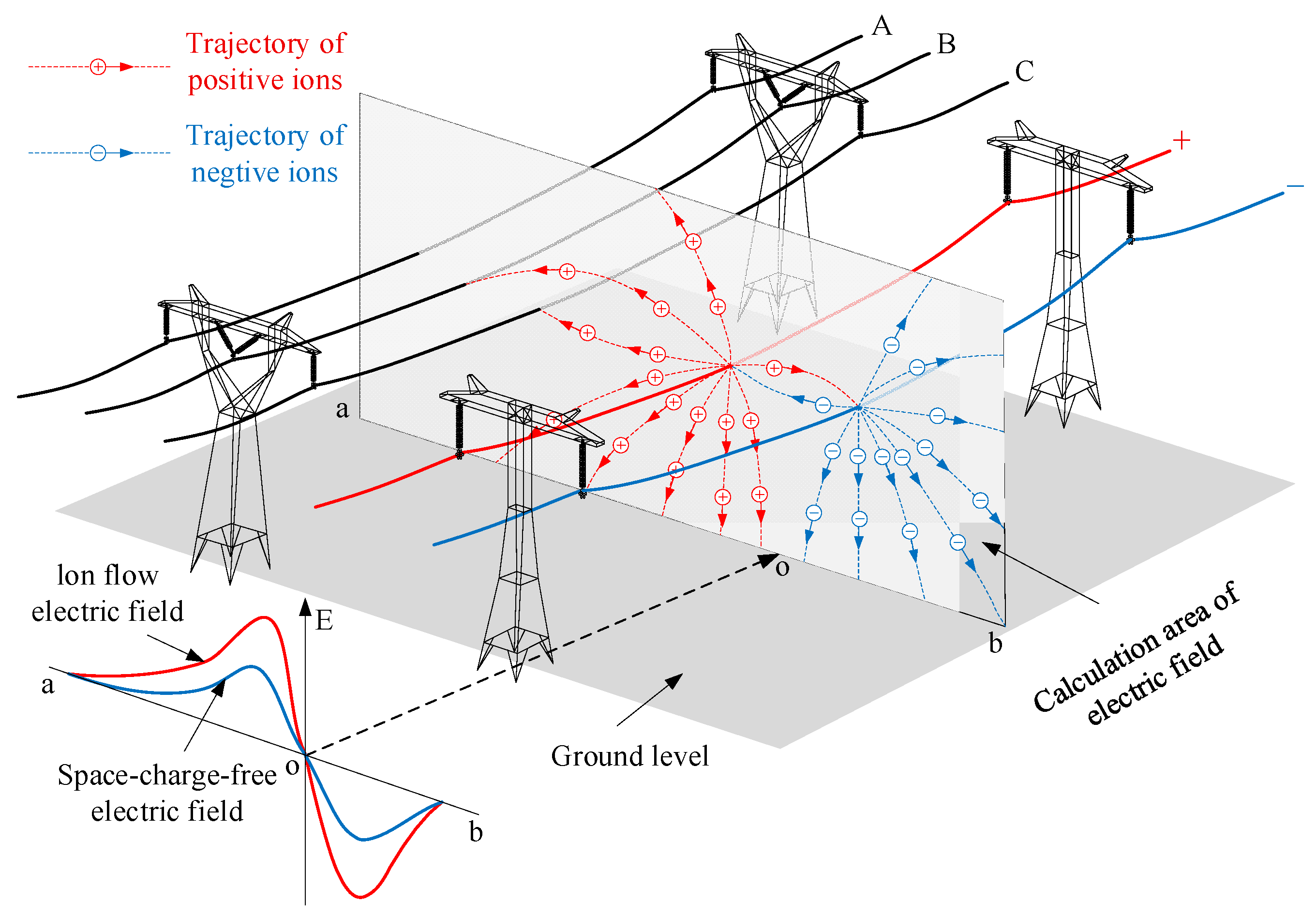
There are two kinds of hybrid transmission lines: HVAC and HVDC lines on one tower, and parallel HVAC and HVDC lines on different towers. Because the electric field at HVDC conductor surface is changed with the power frequency cycle under the influence of HVAC lines, the corona discharge of parallel HVDC conductors is changed, and then space charges distribution is different from HVDC lines without parallel HVAC lines, which is illustrated in Figure 1. A, B, and C represent the three-phase HVAC conductors; “+” and “−” represent the positive and negative HVDC poles. A 2D plane perpendicular to the line shows ion flow trajectories and the ground electric field along segment ab from the DC lines is shown, which clearly manifests the influence of the AC lines. Due to the mutual influence of parallel AC and DC lines [3,4], with challenges posed for fault analysis and corona analysis of the lines additionally [5,6,7], the ion flow field becomes more complicated, which is the superposition of electric field generated by conductor surface charges and space charges due to the corona discharge [8].

In 2022, the transmission and distribution committee of IEEE Power and Energy Society published IEEE standard 2819 on measuring method of electromagnetic environment for the corridor of hybrid transmission lines [9], which can provide guidance for the monitoring of the ground-level electric field in the same corridor. At the same time, the limit value of the ground-level electric field to control the height and corridor width is proposed through human perception experiments [10]. But for the design of hybrid transmission lines, the mutual influence between parallel AC and DC lines on the ground-level electric field must be analyzed on the basis of the numerical calculation in order to obtain a suitable height and corridor width.

Chartier reported the test results of Bonneville power administration and analyzed characteristics of conductor surface gradient in 1981, but there was no calculation method to predict the ground-level electric field [8]. Since then, the effective calculation method has been an important research hotspot. In 1988, Maruvada first calculated the electric field of hybrid transmission lines by using the flux tracing method, which is based on the Deutsch assumption [11]. In 1989, Clairmont adopted the concept of corona saturation degree to analyze the electric field variation of hybrid lines in different configurations [12]. In 1990, Abdel-Salam calculated the electric field without consideration of the space charges’ effect by using the charge simulation method [13]. In 1996, Zhao improved the flux tracing method by treating AC lines as several separate DC voltages during one power-frequency cycle [14], and in 2010, Yang further improved the same method in the time domain along the flux line based on the Deutsch assumption [15]. In 2009, Li proposed the time-domain upwind finite element method without the Deutsch assumption in order to analyze the electric field of hybrid 1000 kV AC and ±800 kV DC lines, and a variable time-step is applied to accelerate the computation process [16]. In 2011, Yin solved the electric field by the charge simulation method and the finite-element method (FEM), and solved the space charges by the time-dependent finite volume method (FVM) [17]. In 2012, Zhou proposed a time-efficient method based on FEM and FVM, where the significant effect of AC corona was analyzed [18]. In 2013, Straumann adopted the discontinuous Galerkin method to the solution of the electric field and discussed the simplification of more complex problems in order to obtain efficient computation [19]. In 2014, Guillod proposed the iterative method of characteristics similar to the flux tracing method, but the Deutsch assumption was abandoned [20]. In 2016, Zhang proposed the time-domain method of characteristics, and the electric field and ion density in the space and time domain were updated [21]. In 2017, Qiao proposed an upwind finite element method combining the domain decomposition technique with high-order elements, and introduced a conductor surface charge density updating strategy based on the corona discharge U–I characteristic curve [22]. Li applied this method to analyze the influence of four different AC conductor arrangements and phase sequence configurations in hybrid transmission lines on the distribution of ground-level electric field [23]. In 2018, Qiao proposed an iterative flux tracing method without the Deutsch assumption, which was more reasonable [24]. In 2018, Ma analyzed the 3D electric field of ±800 kV DC and 500 kV AC parallel lines based on the flux tracing method [25]. In 2019, Tian applied the time-domain mixed-hybrid finite element method to analyze the ion flow field of two typical hybrid transmission lines, improving accuracy and reducing computational burden [26]. In 2020, Xu successfully improved the solution efficiency based on a parallel processing algorithm with fine-grained nodal domain decomposition and an upwind nodal charge conservation method, and the electric field of hybrid lines on one tower was analyzed [27]. With the development of the above method, many characteristics have been obtained in order to understand the ground-level electric field under some special hybrid lines. But the design of hybrid lines, including the height, corridor width and the approach distance, is not emphasized in detail.

In this paper, FEM-FVM is used to solve the ion flow field of hybrid lines in different configurations. Section 2 details the FEM-FVM calculation methods and acceleration techniques. In order to increase the simulation efficiency, the conjugate gradient method with pre-condition treatment (PCG) is applied to treat the coefficient matrix in FEM discretization equation, and generalized minimal residual method (GMRES) with reverse Cuthill-McKee (RCM) and bipartite matching algorithm (BMA) is used to treat the FVM discretization solution. After the efficiency is compared, the ground-level electric field for transmission lines with different configurations is analyzed. Section 3 presents the simulation models and design constraints, focusing on conductor arrangements and electromagnetic limits in China. Finally, Section 4 and Section 5 analyze the design of hybrid lines on one tower and different towers, respectively. The height and the corridor width of double-circuit HVAC lines and one-circuit HVDC lines in the same corridor are obtained, especially the effect of different configurations of AC lines on the design is discussed for hybrid lines on one tower and different towers. The study provides valuable practical recommendations for optimal tower configurations, minimum heights, and corridor widths under various electromagnetic constraints.

2. Calculation Method and Limits

In order to simulate the ion flow field of hybrid lines, the calculation method is introduced first.

2.1. Control Equations and FEM-FVM

The corona of hybrid lines generates a time-dependent bipolar ion flow field problem, which can be described by the following equations:

$${\nabla }^2\phi (t)=-{\displaystyle \frac{{\rho }^{+}(t)-{\rho }^{-}(t)}{{\epsilon }_0}}$$

(1)

$${\displaystyle \frac{\partial {\rho }^{+}(t)}{\partial t}}+\nabla \cdot [{\rho }^{+}(t)k^{+}\nabla \phi (t)]=-{\displaystyle \frac{R{\rho }^{+}(t){\rho }^{-}(t)}{e}}$$

(2)

$${\displaystyle \frac{\partial {\rho }^{-}(t)}{\partial t}}-\nabla \cdot [{\rho }^{-}(t)k^{-}\nabla \phi (t)]=-{\displaystyle \frac{R{\rho }^{+}(t){\rho }^{-}(t)}{e}}$$

(3)

where $\phi$ is the electric potential in time domain, $\rho$ is the charge density in time domain, the superscripts + and − are respectively for positive and negative charges, ${\epsilon }_0$ is the dielectric constant of air, $k$ is the ion mobility, $k^{+}$ = 1.2 × 10⁻⁴ m²/V/s and $k^{-}$ = 1.5 × 10⁻⁴ m²/V/s, R is the ion recombination rate, and e is the electron charge. The influence of air electrical conductivity and air humidity is complicated for charging model establishment [28,29]. Therefore, both air electrical conductivity and humidity are neglected to simplify the model.

The potentials of the DC and AC conductors are set to the applied voltages U_DC and U_AC, while the ground potential is set to zero. The artificial boundary is defined as a semicircle with a radius six times the height of the transmission line, and the low charge density at this boundary has a negligible impact on the potential. The artificial boundary potential $U_{{\Gamma }_3}$ is obtained using the charge simulation method. The boundary conditions of Poisson’s equation are defined as follows:

$$\left\{\begin{array}{c}\phi {|}_{{\Gamma }_1}=U_{DC}\\ \phi {|}_{{\Gamma }_2}=U_{AC}(t)\\ \phi {|}_{{\Gamma }_3}=U_{{\Gamma }_3}(t)\\ \phi {|}_{{\Gamma }_4}=0\end{array}\right.$$

(4)

where ${\Gamma }_1$ is the boundary of the DC conductors, ${\Gamma }_2$ is the boundary of the AC conductors, ${\Gamma }_3$ is the artificial semicircular boundary, and ${\Gamma }_4$ is the ground boundary.

The boundary conditions of the current continuity equations are as follows. As the ionization region thickness around the conductor is neglected, the electric field strength on the conductor surface follows Kaptzov’s assumption, whereby the surface electric field strength equals the corona onset field strength once the applied voltage exceeds the threshold. The conductor surface charge density is initially unknown and is iteratively adjusted at each time step using the secant method [18] to satisfy Kaptzov’s assumption. The consideration of ion drift and the neglect of ion diffusion eliminates the need for boundary conditions on the current continuity equations at the ground and artificial boundaries. If charges flow into the control volume from the outside computational domain, the charge amount is set to zero. If charges flow out, no special treatment is applied.

Because of the coupling of potential and space charges, the iterative process in the time domain is necessary for the solution of the potential in (1) and the space charges in (2) and (3). FEM is applied to discretize Poisson’s Equation (1), and FVM is used to discretize current continuity Equations (2) and (3).

After boundary conditions are applied, (1) can be changed to the following format in the whole calculation area by the treatment of FEM based on triangular meshes:

$$K\phi =F$$

(5)

where K is M*M sparse matrix which is determined by the FEM node relation, $\phi$ is the column vector of node potentials, F is the column vector including the effect of imposed boundary condition and node space charges, and M is the node number in the whole calculation area. The conjugate gradient with pre-conditioning treatment (PCG) is used to solve (5).

Based on the implicit time scheme, (2) can be changed as

$${\rho }_{i,n+1}^{+}={\rho }_{i,n}^{+}-\Delta t\cdot R{\rho }_{i,n+1}^{+}{\rho }_{i,n}^{-}-{\displaystyle \frac{\Delta t}{A_i}}{\displaystyle \sum _{m=1}^{N_i}{\rho }_{i,n+1,m}^{+}{k}^{+}{E}_{i,n,m}{l}_{i,m}}$$

(6)

where A_i, m and N_i are respectively the area, the edge number and the total number of edges in the i-th control volume; the subscript n and n + 1 are respectively for the n-th and n + 1-th time step number; Δt is the time step; l_i,m is the length of the m-th edge in the i-th control volume; ${\rho }_{i,n+1,m}^{+}$ and $E_{i,n,m}$ are respectively the space charge and electric field in the center of the related edge. $E_{i,n,m}$ can be obtained from the upwind control volume using second-order interpolation:

$${\rho }_{i,n+1,m}^{+}={\rho }_{i,n+1,m,up}^{+}+\left[\begin{array}{cc}{x}_{i,m}-x_{i,m,up,c}& y_{i,m}-y_{i,m,up,c}\end{array}\right]\left[\begin{array}{c}{\left({\displaystyle \frac{d{\rho }^{+}}{dx}}\right)}_{i,n+1,m,up}\\ {\left({\displaystyle \frac{d{\rho }^{+}}{dy}}\right)}_{i,n+1,m,up}\end{array}\right]$$

(7)

where ${\rho }_{i,n+1,\mathrm{m},\mathrm{up}}^{+}$ is the average charge density of the m-th edge of the i-th upwind control volume, $x_{i,m,up,c}$ and $y_{i,m,up,c}$ are the coordinates of the center of gravity in the upwind control volume, and the charge density gradient ${(▽{\rho }^{+})}_{i,n+1,\mathrm{m},\mathrm{up}}$ can be obtained by

$$\left[\begin{array}{cc}\Delta x_{\mathrm{i},m,up,1}& \Delta y_{\mathrm{i},m,up,1}\\ \Delta x_{\mathrm{i},m,up,2}& \Delta y_{\mathrm{i},m,up,2}\\ ⋮& ⋮\\ \Delta x_{\mathrm{i},m,up,N}& \Delta y_{\mathrm{i},m,up,N}\end{array}\right]\left[\begin{array}{c}{\left({\displaystyle \frac{d{\rho }^{+}}{dx}}\right)}_{\mathrm{i},n+1,m,up}\\ {\left({\displaystyle \frac{d{\rho }^{+}}{dy}}\right)}_{\mathrm{i},n+1,m,up}\end{array}\right]=\left[\begin{array}{c}{\rho }_{\mathrm{i},n+1,m,up,1}^{+}-{\rho }_{\mathrm{i},n+1,m,up}^{+}\\ {\rho }_{\mathrm{i},n+1,m,up,2}^{+}-{\rho }_{\mathrm{i},n+1,m,up}^{+}\\ ⋮\\ {\rho }_{\mathrm{i},n+1,m,up,N}^{+}-{\rho }_{\mathrm{i},n+1,m,up}^{+}\end{array}\right]$$

(8)

where N is the number of control volumes adjacent to the upwind control volume. Equation (8) can be solved by using the least squares method. Based on (7) and (8), ${\rho }_{i,n+1,m}^{+}$ can be expressed as a polynomial in terms of ${\rho }_{i,n+1,m,up}^{+}$, ${\rho }_{i,n+1,m,up,1}^{+}$, ${\rho }_{i,n+1,m,up,2}^{+}$…${\rho }_{i,n+1,m,up,N}^{+}$. In the mesh with node N₀, Equation (6) can be expanded as:

$$\left\{\begin{array}{c}{A}_{11}{\rho }_{1,n+1}^{+}+A_{12}{\rho }_{2,n+1}^{+}+\dots +A_{1m}{\rho }_{m,n+1}^{+}+\dots +A_{1N_0}{\rho }_{N_0,n+1}^{+}={\rho }_{1,n}^{+}\\ A_{21}{\rho }_{1,n+1}^{+}+A_{22}{\rho }_{2,n+1}^{+}+\dots +A_{2m}{\rho }_{m,n+1}^{+}+\dots +A_{2N_0}{\rho }_{N_0,n+1}^{+}={\rho }_{2,n}^{+}\\ \dots \dots \\ \hspace{1em}\hspace{1em}{A}_{N_{0}1}{\rho }_{1,n+1}^{+}+A_{N_{0}2}{\rho }_{2,n+1}^{+}+\dots +A_{N_{0}m}{\rho }_{m,n+1}^{+}+\dots +A_{N_0{N}_0}{\rho }_{N_0,n+1}^{+}={\rho }_{N_0,n}^{+}\end{array}\right.$$

(9)

Equation (3) can be changed to the similar format as (9) just instead of positive space charges with negative space charges. Then, (2) and (3) can be expressed in the following equations after the treatment of FVM:

$$A\rho =B$$

(10)

which is similar to (5), although each matrix has a different meaning. The coefficient matrix A is not symmetric due to the varying adjacency of each control volume and the asymmetric mutual influence. The GMRES method is used to solve the above equation.

Methods for calculating the hybrid electric field include the finite difference method (FDM) and the flux tracing method, the FEM–FVM and the time-domain upwind finite element method. FDM offers higher computational efficiency but has difficulties in modeling complex models on structured meshes, and local conservation of physical quantities cannot always be guaranteed during the discretization process, particularly in scenarios involving strong convection or sharp gradients. Additionally, the flux tracing method is an analytical solution under the Deutsch assumption, which provides an efficient framework by reducing 2D ion-flow field problems to 1D approximations. While it is computationally efficient and free from numerical oscillations, it fundamentally neglects the distortion of the electric field direction caused by space charge effects. Qiao [24] proposed an iterative flux tracing algorithm, which can progressively reduce Deutsch assumption errors by recursively recalculating space charge-modified electric fields and updating flux line trajectories. The FEM-FVM has two key features: FVM ensures flux conservation, and this method employs iterative computations at each time step to determine charge emission values satisfying the Kaptzov assumption. Both the time-domain upwind finite element method and the FEM-FVM are based on the FEM for solving Poisson’s equation similarly. The time-domain upwind finite element method uses a time-dependent upwind first-order difference method on finite element meshes for the current continuity equations, while FEM-FVM uses a second-order finite volume method based on control volume meshes. In terms of temporal discretization, the time-domain upwind finite element method uses an explicit method, whereas FEM-FVM uses an implicit method. This leads to higher accuracy for FEM-FVM but results in a significant increase in computational load. Therefore, accelerating the FEM-FVM becomes important [30].

2.2. Acceleration Method

According to the previous discussion, Poisson’s equation and current continuity equations can essentially be changed to matrix Equations (5) and (10) after the treatment of FEM-FVM discretization. Because the iteration solution of (5) and (10) in time domain requires significant memory and computational effort, the solution including PCG for FEM discretization and GMRES for FVM discretization is necessary to be improved.

RCM method can reduce the bandwidth of sparse matrices [29]. Therefore, the coefficient matrix of (5) and (10) can be reordered by using RCM, which helps to improve the solution speed. For a 19,000-node calculation, the coefficient matrix of the current continuity equation is reordered by using the RCM method. Figure 2 shows that non-zero elements in the coefficient matrix become more compact after RCM reordering.

The coefficient matrix in (6) and (10) can also be preprocessed by using BMA [31], which reorders the matrices to enhance diagonal dominance. Then (10) can be transformed as:

RPACY = RPB

(11)

where R is the permutation matrix, P is the row scaling matrix, C is the column scaling matrix, and ${Y=C}^{-1}\rho$. After Y is solved, the space charges $\rho$ can be obtained. BMA reduces the condition number of the coefficient matrix, resulting in improved convergence behavior.

The accelerated solution procedure is shown in Figure 3. An inner loop and an outer loop are included in the iteration. The inner loop adjusts the surface charge distribution on AC and DC lines to ensure that the surface electric field does not exceed the corona onset threshold. The outer loop performs time-domain iteration until the convergence condition is reached. The acceleration process is applied to handle the coefficient matrices in the inner loop.

2.3. Validity of Calculation Method

For the model of ±800 kV HVDC and one-circuit 1000 kV HVAC transmission lines in the same corridor, there are 26,721 elements and 13,719 nodes in FEM mesh. The treatment of BMA can significantly reduce the condition numbers of the coefficient matrix.

Table 1. Comparison of the accelerated solution for each iteration.

Calculation Method	Computation Time (s)	Condition Number
PCG (in FEM)	1.056	5.47 × 1018
PCG with BMA (in FEM)	0.173	3.22 × 103
GMRES (in FVM)	0.578	2.63 × 1070
GMRES with BMA and RCM (in FVM)	0.254	108.86

shows the different computation times in a single iteration with a calculation tolerance of 1 × 10⁻¹². For the electric potential calculation, the condition number of FEM discretization equations decreases from 5.47 × 10¹⁸ to 3.22 × 10³, and the computation time is decreased from 1.056 s to 0.173 s after BMA is used. For the space charges calculation, the condition number of the FVM discretization equations decreases from 2.63 × 10⁷⁰ to 108.86, and the computation time is decreased from 0.578 s to 0.254 s after BMA and RCM are used. During the whole iterative process of ground-level electric field, there are approximately 20,000 outer iterations to achieve stable convergence. After acceleration, the total computation time is reduced from 32,680 s to 8,558 s, achieving an acceleration ratio of 3.8.

The actual transmission line model was also calculated using the calculation method. In the Baihetan–Zhejiang transmission lines, the structure of one section is ±800 kV and 500 kV HVDC lines on a single tower, and the AC circuit is a double-circuit vertical arrangement in reverse phase sequence.

Table 2. Comparison of Baizhe Engineering Line Results.

	Max Value of DC Component (kV/m)	Max Value (RMS) of AC Component (kV/m)
CEPRI	2.64	9.85
FEM-FVM with acceleration	2.90	9.71

compares the calculation results of the proposed method with those of the China Electric Power Research Institute (CEPRI) for the engineering model, which shows this method is also applicable to practical engineering [32].

3. Simulation Models and Design Limits

3.1. Simulation Models of Electric Field

The transmission lines considered in this paper include double-circuit 500 kV HVAC lines and one-circuit ±800 kV HVDC lines. HVAC lines can be arranged in an inverted triangular, vertical and horizontal configuration. The conductor parameters are listed in

Table 3. Conductor Parameters.

Voltage	No. of Sub-Conductor	Sub-Conductor	Splitting Distance (mm)
±800 kV	6	JL/G3A-900/75	450
500 kV	4	LGJ-630/45	400

, where the sub-conductor types comply with the standard for “Round wire concentric lay overhead electrical stranded conductors” (GB/T 1179–2017 [33]). There are six kinds of phase sequence arrangements for double-circuit HVAC lines. The phase sequence of the left circuit is fixed as illustrated in Figure 4 and Figure 5, and the phase sequences of the right circuit are listed in

Table 4. Phase sequence arrangement.

Line Number	I	II	III	IV	V	VI
1/2/3	C/B/A	C/A/B	B/A/C	B/C/A	A/B/C	A/C/B

.

For double-circuit 500 kV HVAC lines and one-circuit ±800 kV HVDC lines on different towers in the same corridor, illustrated in Figure 5, the minimum horizontal distance S between AC lines and DC lines is determined to be 20 m [34].

3.2. Design Limits

The limit values of the electric field, ion current density, audible noise (AN) and radio interference (RI) adopted in the paper in China are listed in

Table 5. Electromagnetic environmental limits.

Factor	Situation	500 kV	±800 kV
Electric field (kV/m)	Non-residential	10	dry	30
			wet	36
	Residential	7	dry	25
			wet	30
Ion current density (nA/m2)	Non-Residential	-	100
	Residential	-	80
AN (dB(A))	sunny day	-	45
	rain	55	-
RI (dB(μV/m))	80%–80%	55	58

, which are used to determine the conductor height and other geometry configuration for hybrid transmission lines in non-residential area or residential area [35]. The limit of RI or AN is at the position 20 m outside the positive pole for HVDC lines or outside the outer phase line for HVAC lines. RI is calculated using the CISPR method, and AN using the BPA method. In Table 5, weather conditions include dry and wet states, with corresponding surface roughness coefficients of 0.47 and 0.37, respectively. These values are used in the Peek equation to calculate the corona onset electric field of stranded wire. For AN, “sunny day” and “rain” refer to weather conditions. For RI, the 80%–80% rule refers to a statistical method ensuring that 80% of the appliances being tested meet the specified radio noise limit with at least 80% confidence [36].

In China, there is no national standard for the electromagnetic environment of HVAC-HVDC hybrid transmission lines, but the limits for separate HVAC lines and HVDC lines have been established. The normalized AC and DC electric field using their respective control values to determine the limit for hybrid electric fields is recommended [34]

$$C_H(x)={\displaystyle \frac{E_{DC}(x)}{E_{DCLim}}}+{\displaystyle \frac{E_{AC}(x)}{E_{ACLim}}}$$

(12)

where $E_{DCLim}$ and $E_{ACLim}$ are the limits for DC and AC transmission lines, respectively, $C_H$ denotes the normalized value of the hybrid electric field. The hybrid electric field under the hybrid lines must satisfy

$$C_H\le 1$$

(13)

Experimental studies on human perception and transient shock sensations under electric fields with varying proportions of AC and DC components indicate that the above method can be reliably used in engineering designs [10,23,37].

4. HVDC and HVDC Lines on One Tower

4.1. Main Design Constraint Factor

It is necessary to obtain the main design constraint that has the greatest impact on engineering design due to electromagnetic environment, in other words, to determine the most important factor among electric field, RI and AN during the design of HVAC-HVDC hybrid transmission lines. If the value of the factor is under the permissible limit, other electromagnetic factors will not be paid attention to in terms of the electromagnetic environment.

In order to obtain the main design constraint, the height H in Figure 4 is increased until only one factor is beyond the limit, which is the significant factor. Taking phase sequence I of double-circuit 500 kV AC lines as an example, the results of normalized hybrid electric field, ion current density, RI and AN for three different AC arrangements are shown in

Table 6. The main design constraint factor for hybrid lines is on one tower.

Design Indicator			Triangular	Vertical	Horizontal
Increased Height (m)			10	10	14
CH	Non-residential	Dry	1.23	1.16	0.65
		Wet	1.26	1.19	0.65
	Residential	Dry	1.75	1.16	0.90
		Wet	1.79	1.19	0.90
Ion current density (nA/m2)		Dry	0.85	0.85	1.44
		Wet	1.02	0.98	1.82
RI @ DC side (dB(μV/m))			49.96	46.75	61.78
RI @ AC side (dB(μV/m))			47.59	46.2	55.92
Constraint factor			E Field	E Field	RI

. Because the ion current density is very low due to the shielding effect of AC lines, it can be neglected during the design of hybrid lines on one tower. For the inverted triangular arrangement and vertical arrangement, the normalized hybrid electric field is more than 1; therefore, the electric field is the main constraint factor during the design. However, for the horizontal arrangement, the main design constraint factor is RI. More calculations show that the main factor influencing the design does not change with the variation of the phase sequence.

4.2. Minimum Height Above the Ground

It is necessary to understand the minimum height for different structures in order to provide design references. By continuously increasing H and calculating the electromagnetic environment of the model, the minimum height is determined when all design indicators in Table 6 meet their respective limit requirements.

Table 7. Minimum height for three arrangements of hybrid lines on one tower.

Area Type	Arrangement	I	II	III	IV	V	VI
Non-residential	Triangular (m)	12.5	12	11	11	12	11
	Vertical (m)	12	12	12	12	12	12
	Horizontal (m)	32	31	31	28	32	27
Residential	Triangular (m)	16.5	15	14	14	16.5	14
	Vertical (m)	15	15	16	15	16	15
	Horizontal (m)	32	31	31	28	32	27

presents the minimum height corresponding to 6 kinds of phase sequences under inverted triangular, vertical and horizontal arrangements. For horizontal arrangement, the minimum height is excessively high due to RI. Therefore, horizontal arrangement is not recommended for HVAC-HVDC lines on one tower, and it is not included in the following discussion.

In non-residential areas, phase sequences III, IV and VI with a minimum height of 11 m are recommended for the inverted triangular arrangement. For the vertical arrangement, the impact of phase sequence on minimum ground clearance is negligible, and the minimum height of 12 m is suitable for all sequences.

In residential areas, phase sequences III, IV and VI with a minimum height of 14 m are also recommended for the inverted triangular arrangement. For vertical arrangement, phase sequences I, II, IV and VI are recommended with a minimum height of 15 m.

As an example, Figure 6 illustrates the ground-level electric field for two kinds of arrangements with phase sequence I in non-residential areas, where the zero X coordinate is the center of the AC transmission circuit. The hybrid electric field distribution of HVAC-HVDC lines on one tower is respectively illustrated as AC electric field, DC electric field and the superposition of AC and DC electric field. The results of the inverted triangular arrangement when H is 12.5 m are illustrated in Figure 6a. The results of the vertical arrangement when H is 12 m are illustrated in Figure 6b. For the inverted triangular and vertical arrangement, AC peaks are closer to the center, while DC peaks are far from the center. The staggered peak distribution is helpful to keep the normalized hybrid electric field below the limit. If the arrangement of conductors is the same, the peak values are higher under wet conditions than under dry conditions, because the corona onset electric field under wet conditions is lower.

4.3. Corridor Width

Two key factors must be considered when determining the corridor width for hybrid transmission lines. The first one is the horizontal distance outside the edge conductor, which is 5 m for a 500 kV AC line side and 7 m for a ±800 kV DC line side [38,39]. The other one is the ground-level electric field. In China, the AC electric field should not be stronger than 4 kV/m, and the DC electric field should not be stronger than 15 kV/m at the edge of the corridor. Therefore, the corridor width is determined according to the normalized hybrid electric field

$$C_W={\displaystyle \frac{E_{AC}}{4}}+{\displaystyle \frac{E_{DC}}{15}}$$

(14)

where at the edge of the corridor width

$$C_W=1$$

(15)

Figure 7 shows the hybrid electric field when the height H is 13 m. The corridor width is from the position x₃ to x₂ for the inverted triangular arrangement and from x₄ to x₁ for the vertical arrangement. In point of hybrid electric field, the corridor width of inverted triangular arrangement is smaller than that of vertical arrangement, but the corridor width gets larger based on the position of edge conductor, which is shown in

Table 8. Corridor width for hybrid lines on one tower.

Phase Sequence	Triangular (m)		Vertical (m)
	By CW	By Edge Conductors	By CW	By Edge Conductors
I	39	48	47	35
II	38
III
IV
V
VI	37

. For six kinds of phase sequences, respectively, determined by the edge conductors and by normalized hybrid electric field, the phase sequence variation has a small effect on the corridor width. Finally, the inverted triangular arrangement is not recommended in reality, and the vertical arrangement is recommended, where the corridor width is determined by the normalized hybrid electric field C_W.

5. Hvdc and Hvac Lines on Different Towers

5.1. Main Design Constraint

Table 9. The main design constraint factor for AC-DC lines on different towers.

Design Indicator			Triangular	Vertical	Horizontal
CH	Non-residential	Dry	1.13	1.09	1.09
		Wet	1.14	1.12	1.17
	Residential	Dry	1.59	1.51	1.44
		Wet	1.61	1.56	1.49
Ion current density (nA/m2)		Dry	43.05	35.64	36.74
		Wet	86.81	81.94	82.24
AN @ DC side (dB(A))		Dry	42.67	43.01	47.95
		Wet	42.97	41.17	41.58
AN @ AC side (dB(A))		Dry	41.88	42.59	48.75
		Wet	36.30	35.96	35.66
RI @ DC side (dB(μV/m))			54.36	50.68	51.02
RI @ AC side (dB(μV/m))			41.91	42.85	51.55
Constraint factor			E Field	E Field	E Field

lists the electric field, RI and AN for three kinds of arrangements in Figure 5, where the horizontal approaching distance S is 20 m, with the height of AC lines (Hac) 11 m and the height of DC lines (Hdc) 17 m. In non-residential areas, only the C_H value in Table 9 exceeds the limits in Table 5, indicating that the hybrid electric field is the main design constraint. In residential areas, both the ion current density under wet conductor conditions and C_H exceed the limits, so both the electric field and ion current density are the main design constraints. Calculation results for other phase sequences indicate that the constraint factor is not changed with phase sequence. Because the electric field is stronger under wet conditions than under dry conditions, the following discussion on the approaching distance, minimum height and corridor width will be under wet conditions.

5.2. Minimum Height and Corridor Width

For HVAC-HVDC lines on different towers, extensive calculations are required to determine the minimum height of AC and DC lines, represented by Hac and Hdc. The calculation procedure is shown in Figure 8. A set of calculations by fixing Hac (or Hdc) while varying Hdc (or Hac) are completed one by one.

For phase sequence I, the normalized hybrid electric fields with a wet conductor are shown in Figure 9. The maximum C_H in the AC area meets the limit requirements under the case of Hac 13 m and Hdc 16 m, and the maximum C_H in the DC area under the case of Hac 11 m and Hdc 19 m is at the threshold. Therefore, the minimum heights are respectively determined as Hac 13.5 m and Hdc 19.5 m with the maximum C_H 0.95.

The hybrid electric fields for six kinds of phase sequences under three arrangements are calculated. The minimum heights in non-residential and residential areas are presented in

Table 10. Minimum height and corridor width for AC-DC lines on different towers.

Arrangement	Area	Phase Sequence	Hac (m)	Hdc (m)	Corridor Width (m)
Triangular	Non-residential	I	13	19.5	108
		II	11.5	19.5	108
		III	11.5	19	107
		IV	12	19	108
		V	13	19	107
		VI	12	19	108
	Residential	I	18	23	105
		II	16.5	23	105
		III	15	22	105
		IV	16	22.5	104
		V	18	23	105
		VI	16	22.5	105
Vertical	Non-residential	I	14	19	104
		II	14	19.5	104
		III	15	19	104
		IV	14	19	104
		V	15	19	105
		VI	14	18	106
	Residential	I	17	22.5	101
		II	18	23	98
		III	19	23	101
		IV	19	24	99
		V	21	25	101
		VI	19	24	99
Horizontal	Non-residential	I	13	20	127
		II	13	21	127
		III	13	20	126
		IV	12	20	127
		V	12	20	127
		VI	12	21	127
	Residential	I	15	25	124
		II	17	25	70 (101)
		III	17	24	101
		IV	17	25	70 (101)
		V	16	24	121
		VI	17	24	99 (101)

with the corresponding corridor widths.

In non-residential areas, phase sequence III for the inverted triangular arrangement is recommended, where the minimum height is 11.5 m for AC lines and 19 m for DC lines. The phase sequence VI for vertical arrangement is recommended, where the minimum height is 14 m for AC lines and 18 m for DC lines. The recommended phase sequences for horizontal arrangement are IV and VI, corresponding to the minimum height of 12 m for AC lines and 20 m for DC lines.

In residential areas, phase sequence III is recommended for the inverted triangular arrangement, where the minimum height is 15 m for AC lines and 22 m for DC lines. The phase sequence I for the vertical arrangement is recommended with a minimum height of 17 m for AC lines and 22.5 m for DC lines. The phase sequence I or V for the horizontal arrangement is recommended with a minimum height of 15 m for AC lines and 25 m for DC lines, or 16 m for AC lines and 24 m for DC lines.

For the inverted triangular and vertical arrangements, the corridor widths determined by edge conductors (93.5 m and 80.5 m, respectively) are smaller than those based on the hybrid electric field. Therefore, for these two arrangements, the corridor width should be determined by the hybrid electric field. However, for the horizontal arrangement, the corridor width determined by edge conductors is 101 m, which is larger than the results of phase sequences II, IV and VI. In order to discuss it in detail, the C_W of phase sequences IV and V is illustrated in Figure 10. The width for phase sequence V according to (16) is the distance between A and C, while for phase sequence IV, the width is the distance between B and C. It means that the electric field at the AC side of the phase sequence IV is very low, which is not a decisive factor for the corridor width. Therefore, the corridor width should be determined by the position of the outer AC line.

From the perspective of the minimum height, the inverted triangular arrangement is the best. In contrast, the vertical arrangement requires a higher height for AC lines, and the horizontal arrangement requires a higher height for DC lines.

From the perspective of the corridor width, the vertical arrangement of AC lines is more advantageous among the three arrangements, because the corridor width is the smallest. For the case including residential buildings, which is not considered in this paper, the electric field on the platform of the buildings where people can reach should also be calculated, because the new standard about DC electric field was published in 2020 [40].

5.3. Impact of Approaching Distance

In order to analyze the influence of the approaching distance, the heights of phase sequence I in non-residential areas in Table 10 are adopted. The normalized hybrid electric fields are shown in Figure 11 for different approaching distances of 20  m, 30  m, 40  m, 50  m, 60  m and 70  m.

When the approaching distance is larger than 60 m, the normalized hybrid electric field is almost unchanged with the variation of S. The approaching distance is smaller, the more significant the coupling between AC lines and DC lines is. For vertical arrangement and horizontal arrangement, the maximum of the normalized electric field C_Hmax decreases significantly with the increase of approaching distance when S is smaller than 40 m. But for the inverted triangular arrangement, the maximum of the normalized electric field decreases slightly. Therefore, the minimum height should be related to the approaching distance between AC lines and DC lines.

6. Conclusions

In order to effectively analyze the electric field of hybrid HVAC and HVDC transmission lines in the same corridor, the FEM-FVM method is accelerated by the conjugate gradient method and generalized minimal residual method with pre-conditioning treatment. With the help of BAM and RCM, the computation speed can be increased by more than 3.8 times.

One-circuit ±800 kV DC lines and double-circuit 500 kV AC lines with inverted triangular, vertical and horizontal configurations under six kinds of different phase sequences are analyzed, and the calculation results, including hybrid electric field, ion current density, audible noise, and radio interference, are obtained. Based on the limit values in China, the main design constraint factor is determined. For HVAC-HVDC lines on one tower, the hybrid electric field is the most important factor for inverted triangular and vertical AC arrangements, but RI is the main constraint factor for horizontal arrangements. For HVAC-HVDC lines on different towers, the hybrid electric field in non-residential areas is the main factor influencing the design, and ion current density should be additionally considered in residential areas.

Different conductor arrangements can result in different results of minimum height and corridor width due to the distribution of hybrid electric fields. For HVAC-HVDC lines on one tower, the inverted triangular arrangement is the best choice to obtain lower height and smaller corridor width in the view of electric field, with recommended minimum heights of 11 m (phase sequence III, non-residential) and 14 m (phase sequence III, residential), and a corridor width of 37–39 m. For HVAC-HVDC lines on different towers, the phase sequence III inverted triangular configuration is better to obtain lower minimum height (Hac = 11.5 m and Hdc = 19 m for non-residential area, Hac = 15 m and Hdc = 22 m for residential area). The vertical arrangement is recommended to obtain a smaller corridor width of HVAC-HVDC lines in reality, and the horizontal arrangement is not recommended due to a wider corridor width. For vertical and horizontal configurations, increasing the approaching distance S within 30–40 m is recommended to effectively reduce the C_Hmax. For the inverted triangle configuration, increasing S has a limited impact on reducing C_Hmax and the minimum approaching distance of S = 20 m is recommended.

References

1. Sarma, M.P. Corona Performance of High-Voltage Transmission Lines; Crown Publication cc: Johannesburg, South Africa, 2011; pp. 12–13. [Google Scholar]
2. Larruskain, D.M.; Zamora, I.; Abarrategui, O.; Aginako, Z. Conversion of AC distribution lines into DC lines to upgrade transmission capacity. Electr. Power Syst. Res. 2011, 81, 1341–1348. [Google Scholar] [CrossRef]
3. El-Deen, S.K.; Abdel-Salam, M.; El-Mohandes, M.T. Analysis of corona on hybrid DC and AC overhead transmission lines. IEEE Trans. Plasma Sci. 2023, 51, 2926–2941. [Google Scholar] [CrossRef]
4. Hedtke, S.; Bleuler, P.; Franck, C.M. Outdoor investigation of the corona characteristics and audible noise of a hybrid AC/DC overhead line. IEEE Trans. Power Del. 2021, 36, 3309–3317. [Google Scholar] [CrossRef]
5. Fayazi, M.; Saffarian, A.; Joorabian, M.; Monadi, M. Analysis of induced components in hybrid HVAC/HVDC transmission lines on the same tower for various fault conditions. Electr. Power Syst. Res. 2024, 226, 109884. [Google Scholar] [CrossRef]
6. Fayazi, M.; Saffarian, A.; Joorabian, M.; Monadi, M. An AI-based fault detection and classification method for hybrid parallel HVAC/HVDC overhead transmission lines. Electr. Power Syst. Res. 2025, 238, 111083. [Google Scholar] [CrossRef]
7. Xia, J.; Ma, Z.; He, Z.; He, X.; Zhao, L.; Shen, B.; He, K.; Bian, X. Experimental and theoretical study of corona inception threshold in rod to plane electrodes under AC/DC combined voltage: Phase corresponding to AC voltage. IEEE Trans. Dielectr. Electr. Insul. 2023, 30, 403–412. [Google Scholar] [CrossRef]
8. Chartier, V.L.; Sarkinen, S.H.; Stearns, R.D.; Burns, A.L. Investigation of corona and field effects of AC/DC hybrid transmission lines. IEEE Trans. Power App. Syst. 1981, PAS-100, 72–80. [Google Scholar] [CrossRef]
9. IEEE Standard 2819-2022; IEEE Recommended Practice for Measuring Method of Electromagnetic Environment for the Corridor of High-Voltage Overhead Power Transmission Lines in Parallel Mixed with Alternating Current and Direct Current. IEEE: New York, NY, USA, 2022.
10. Xie, L.; Lu, J.; Yang, Y.; Wu, G.; Ju, Y. Study on human perception experiments and design limits of the hybrid electric field of parallel HVAC and HVDC transmission lines. Proc. CSEE 2024, 44, 776–789. [Google Scholar]
11. Maruvada, P.S.; Drogi, S. Field and ion interactions of hybrid AC/DC transmission lines. IEEE Trans. Power Del. 1988, 3, 1165–1172. [Google Scholar] [CrossRef]
12. Clairmont, B.A.; Johnson, G.B.; Zaffanella, L.E.; Zelingher, S. The effect of HVAC-HVDC line separation in a hybrid corridor. IEEE Trans. Power Del. 1989, 4, 1338–1350. [Google Scholar] [CrossRef]
13. Abdel-Salam, M.; El-Mohandes, M.T.; El-Kishky, H. Electric field around parallel DC and multi-phase AC transmission lines. IEEE Trans. Electr. Insul. 1990, 25, 1415–1422. [Google Scholar] [CrossRef]
14. Zhao, T.; Sebo, S.A.; Kasten, D.G. Calculation of single phase AC and monopolar DC hybrid corona effects. IEEE Trans. Power Del. 1996, 11, 1454–1462. [Google Scholar] [CrossRef]
15. Yang, Y.; Lu, J.; Lei, Y. A calculation method for the hybrid electric field under UHVAC and UHVDC transmission lines in the same corridor. IEEE Trans. Power Del. 2010, 25, 1146–1153. [Google Scholar] [CrossRef]
16. Li, W.; Zhang, B.; He, J.; Zeng, R.; Li, X.; Wang, Q. Calculation of ion flow field of AC-DC hybrid transmission line. IET Gener. Transm. Distrib. 2009, 3, 911–918. [Google Scholar] [CrossRef]
17. Yin, H.; He, J.; Zhang, B.; Zeng, R. Finite volume-based approach for the hybrid ion-flow field of UHVAC and UHVDC transmission lines in parallel. IEEE Trans. Power Del. 2011, 26, 2809–2820. [Google Scholar] [CrossRef]
18. Zhou, X.; Cui, X.; Lu, T.; Zhen, Y.; Luo, Z. A time-efficient method for the simulation of ion flow field of the AC-DC hybrid transmission lines. IEEE Trans. Magn. 2012, 48, 731–734. [Google Scholar] [CrossRef]
19. Straumann, U.; Franck, C.M. Ion-flow field calculations of AC/DC hybrid transmission lines. IEEE Trans. Power Del. 2013, 28, 294–302. [Google Scholar] [CrossRef]
20. Guillod, T.; Pfeiffer, M.; Franck, C.M. Improved coupled ion-flow field calculation method for AC/DC hybrid overhead power lines. IEEE Trans. Power Del. 2014, 29, 2493–2501. [Google Scholar] [CrossRef]
21. Zhang, B.; Mo, J.; He, J.; Zhuang, C. A time-domain approach of ion flow field around AC–DC hybrid transmission lines based on method of characteristics. IEEE Trans. Magn. 2016, 52, 7205004. [Google Scholar] [CrossRef]
22. Qiao, J.; Zou, J.; Yuan, J.; Li, B. Electric Field Calculation of HVAC and HVDC Transmission Lines on the Same Tower With Domain Decomposition Method and High Order Element. Power Syst. Technol. 2017, 41, 335–341. [Google Scholar]
23. Li, B.; Qiao, J.; Zou, J.; Yuan, J. Analysis of Configuration and Corridor Width of HVAC and HVDC Transmission Lines on Same Tower. Power Syst. Technol. 2017, 41, 353–359. [Google Scholar]
24. Qiao, J.; Zhang, P.; Zhang, J.; Lu, Y.; Zou, J.; Yuan, J.; Huang, S. An iterative flux tracing method without Deutsch assumption for ion-flow field of AC/DC hybrid transmission lines. IEEE Trans. Magn. 2018, 54, 7200504. [Google Scholar] [CrossRef]
25. Ma, A.; Chen, J. Analysis of the three-dimensional hybrid electric fields and the related electrostatic induction effects of 800 kV DC and 500 kV AC parallel transmission lines considering environmental factors. Electr. Power Syst. Res. 2018, 163, 638–646. [Google Scholar] [CrossRef]
26. Tian, Y.; Huang, X.; Tian, W.; Cao, W.; Zhu, Y.; Zhao, L.; Zhang, Y. Time-domain mixed hybrid finite element method for analyzing ion-flow field of HVDC and HVAC transmission lines. Electr. Mach. Control 2019, 23, 85–94. [Google Scholar]
27. Xu, Q.; Liu, P.; Dinavahi, V. Parallel finite element computation of time-varying ionized field around hybrid AC/DC lines via fine-grained domain decomposition. IEEE Access 2020, 8, 91248–91256. [Google Scholar] [CrossRef]
28. Shen, N.; Su, Z.; Lu, T. The influence of charge characteristics of suspension droplets on the ion flow field in different temperatures and humidity. Plasma Sci. Technol. 2022, 24, 044004. [Google Scholar] [CrossRef]
29. Shen, N.; Su, Z.; Zou, Y.; Lu, T. Influence of humidity on the charge characteristics of suspension droplets and the characteristics of ion flow field. Trans. China Electrotech. Soc. 2022, 37, 3422–3430. [Google Scholar]
30. Ferziger, J.H.; Perić, M. Computational Methods for Fluid Dynamics, 3rd ed.; Springer: Berlin, Germany, 2002. [Google Scholar]
31. Duff, I.S.; Koster, J. On algorithms for permuting large entries to the diagonal of a sparse matrix. SIAM J. Matrix Anal. Appl. 2001, 22, 973–996. [Google Scholar] [CrossRef]
32. Xie, L. Study on Electromagnetic Environment of Baihetan-Zhejiang ±800 kV Transmission Line with Other DC and AC Transmission Lines on the Same Tower or Parallel in the Adjacent Corridors; Technical Report; China Electric Power Research Institute: Beijing, China, February 2023. [Google Scholar]
33. GB/T 1179-2017; Round Wire Concentric Lay Overhead Electrical Stranded Conductors. General Administration of Quality Supervision, Inspection and Quarantine of the People’s Republic of China: Beijing, China, 2017.
34. Wu, G.; Yu, J.; Guo, X.; Ju, Y. Study on least approaching distances between ±800 kV DC transmission line and 1000 kV AC transmission line in a hybrid corridor. Electr. Power 2007, 40, 22–26. [Google Scholar]
35. China DL/T 5582-2020; Code for Electrical Design of Overhead Transmission Lines. China Planning Press: Beijing, China, 2020.
36. CISPR Publication 18-2; Radio Interference Characteristics of Overhead Power Lines and High-Voltage Equipment, Part 2: Methods of Measurement and Procedure for Determining Limits. IEC: Geneva, Switzerland, 2017.
37. China T/CEC 688–2022; Design and Control Standard for Hybrid Electric Field of EHV/UHV Transmission Lines. CEC: Beijing, China, 2022.
38. China GB 50545; Code for Design of 110 kV~750 kV Overhead Transmission Line. China Planning Press: Beijing, China, 2010.
39. China GB 50790; Code for Design of ±800 kV DC Overhead Transmission Line (Partial Revision). China Planning Press: Beijing, China, 2020.
40. China GB 39220; Limits and Monitoring Methods of Total Electric Field of DC Transmission Project. China Environmental Publishing Group Co., Ltd.: Beijing, China, 2020.
Figure 1. Electric field and space charges of hybrid AC and DC transmission lines on different towers.
Energies 18 03657 g001
Figure 2. Comparison of coefficient matrix before and after RCM reordering: (a) Unsorted; (b) RCM-Sorted.
Energies 18 03657 g002
Figure 3. FEM-FVM accelerated solution procedure.
Energies 18 03657 g003
Figure 4. HVDC and HVAC lines on one tower: (a) Inverted Triangular Arrangement; (b) Vertical Arrangement; (c) Horizontal Arrangement.
Energies 18 03657 g004
Figure 5. HVDC and HVAC lines on different towers: (a) Inverted Triangular Arrangement; (b) Vertical Arrangement; (c) Horizontal Arrangement.
Energies 18 03657 g005
Figure 6. Lateral distribution of ground-level hybrid electric field under DC-AC lines on one tower: (a) Inverted Triangular Arrangement; (b) Vertical Arrangement.
Energies 18 03657 g006
Figure 7. Normalized hybrid electric field for AC-DC lines on one tower with inverted triangular and vertical arrangements (sequence I).
Energies 18 03657 g007
Figure 8. Flowchart to determine the minimum height of AC lines and DC lines.
Energies 18 03657 g008
Figure 9. Normalized hybrid electric field for AC-DC lines on different towers with inverted triangular arrangement (phase sequence I).
Energies 18 03657 g009
Figure 10. Normalized electric field for phase sequences Ⅳ and Ⅴ with horizontal arrangement.
Energies 18 03657 g010
Figure 11. Normalized hybrid electric field for AC-DC lines (sequence I) with different approaching distance: (a) Inverted Triangular Arrangement; (b) Vertical Arrangement; (c) Horizontal Arrangement.
Energies 18 03657 g011