Exploration of Unsupervised Deep Learning-Based Gear Fault Detection for Wind Turbine Gearboxes

Abstract

Gearboxes are critical mechanical components in various modern constructions, including wind turbines, making their real-time monitoring and the prevention of major failures essential. Machine learning (ML) offers a precise and robust method for early-stage failure detection and efficient gear monitoring during operation, with computational efficiency that allows for use on edge devices. This article presents a method for detecting surface damage on gear teeth using unsupervised machine learning. Using only experimentally measured vibrational signals from a healthy gearbox as a training set, novel neural network architectures, including convolutional and recurrent autoencoders, were employed and compared with a classical dense autoencoder. The study confirmed the effectiveness of these methods in gear transmission diagnostics and demonstrated the potential for achieving high-quality classification metrics using unsupervised learning.

1. Introduction

Wind turbines have become a cornerstone of the global shift toward renewable energy. Yet, their long-term viability hinges on the reliability of critical mechanical subsystems, particularly the gearbox. As a central and high-cost component, the gearbox is prone to faults due to variable loading conditions, harsh operating environments, and complex dynamic interactions. These failures, although statistically rare—with serious gearbox faults occurring at a rate of 0.03 per turbine per year—can result in severe consequences, including unplanned downtimes of over 18 days and substantial maintenance costs [1]. Consequently, early fault detection in wind turbine gearboxes is vital to ensure operational reliability and to minimize life cycle costs.

Traditional condition monitoring methods for wind turbine gearboxes have focused on physics-based approaches, particularly vibration and thermal analyses. Frequency-domain analyses have been applied to simulated gearbox models to detect gear defects via characteristic spectral signatures [2], while vibration-based methods have demonstrated real-world efficacy in identifying gear and bearing faults in utility-scale turbines [3]. Thermal monitoring techniques, such as those incorporating SCADA-derived thermal network models, offer complementary insights by detecting anomalies in heat dissipation patterns [4]. However, these methods often require expert knowledge and are limited in capturing complex, nonlinear fault dynamics.

With the increasing availability of SCADA and sensor data, data-driven methods have emerged as powerful alternatives or supplements to traditional techniques. Early applications used statistical learning models such as Support Vector Machines (SVMs) and Dynamic Principal Component Analysis (DPCA) to detect gear anomalies, with notable success [5,6]. More recently, machine learning (ML) and deep learning (DL) approaches have shown great promise in identifying early signs of failure from operational data. For example, artificial neural networks (ANNs) have been used to model nominal gearbox behavior, flagging anomalies based on temperature deviations [7]. Advanced models such as Joint Variational Autoencoders (JVAEs) and Sparse Isolation Encoding Forests (SIEFs) extend this capability by providing robust unsupervised anomaly detection without requiring labeled failure data [8,9]. These approaches are particularly attractive in industrial contexts where fault data is scarce.

Deep learning architectures have rapidly evolved to accommodate the temporal and multivariate nature of SCADA signals. Traditional convolutional neural networks (CNNs) have been applied to vibration data for local feature extraction [10], while graph-based models such as graph convolutional networks (GCNs) [11] and spatio-temporal hybrids have further advanced the field. Notable examples include wavelet-decomposed graph inputs [12], spatiotemporal fusion networks combining GCNs and LSTMs [13], and sandwich-style architectures integrating CNNs and GCNs for blade and bearing fault classification [14]. Although primarily applied to photovoltaic systems, the technique by Arifeen et al. [15]—a graph-variational convolutional autoencoder—offers a transferable deep learning framework capable of learning complex spatiotemporal features, suggesting potential for future applications in wind turbine gearbox monitoring. These models effectively capture spatial and temporal dependencies, providing high diagnostic accuracy.

Yet, practical deployment of these sophisticated models remains challenging. High-capacity networks demand large volumes of high-quality, labeled training data—a luxury not typically available in industrial wind farms. Failures are rare, labeled datasets are expensive to obtain, and operational variability complicates model generalization. This scarcity of annotated fault data leads to overfitting and limited applicability of complex models in low-data environments.

To address these constraints, more compact and data-efficient deep learning architectures, such as autoencoders, have gained attention. Autoencoders, designed to learn compressed representations of input data by reconstructing normal operational states, are especially suited for unsupervised fault detection [16,17,18]. They require no failure labels and can effectively highlight deviations from healthy patterns by analyzing reconstruction errors. CNN-based autoencoders offer resilience to noise and can model periodic SCADA patterns [19,20], while GRU-based variants capture long-term temporal dependencies with fewer parameters than traditional LSTMs, making them ideal for uneven or sparse time-series data.

In our previous investigation [21], as a part of it, we explored a standard fully connected autoencoder for anomaly detection. While it provided interesting outcomes in data dimensionality reduction, allowing various semi-supervised algorithms to be explored in the latent layer, its overall performance was far from perfect. In practical industrial environments, vibrational data from gear systems is often imbalanced. The majority of this data reflects normal operating conditions, while only a small percentage indicates various failure modes. This imbalance, along with the limited availability of labeled fault data—especially for early-stage or rare failure types—creates a significant challenge for training supervised or semi-supervised deep learning models. To address these challenges, this study investigates a truly unsupervised approach, using autoencoders built on a feed-forward neural network, convolutional neural networks (CNNs) and gated recurrent units (GRUs). These architectures can learn compact and meaningful representations of normal operating conditions without needing labeled failure examples. By modeling only healthy behaviors, the autoencoders can effectively identify deviations suggestive of faults, including early signs of pitting, by analyzing reconstruction errors. This approach aligns with the realities of gear diagnostics, where the scarcity of fault data and the necessity for early detection require models that can generalize well with limited supervision. In our current research, we focus on detecting the slightest signs of initial pitting under laboratory conditions. This work will be expanded in future studies to apply to real gearboxes. Therefore, in this paper, we revisit our experimentally collected data and explore various architectures of autoencoders, in order to find the optimal one. As the signal in question resembles a time series, we utilize specialized architectures that have been proved to be more proficient in processing such data—convolutional networks and recurrent networks. The paper is organized as follows: in Section 2 we describe how the experiment was conducted, the data were acquired, and we describe the preprocessing of the measured signal. Then in Section 3 we introduce all three autoencoder architectures we tested—the fully connected, being the baseline; convolutional; and recurrent. In Section 4 we analyze the problem of finding the optimal threshold, where we classify a signal as healthy or faulty, and finally in Section 5 we conclude the paper.

2. Materials and Methods

2.1. Experimental Data Acquisition

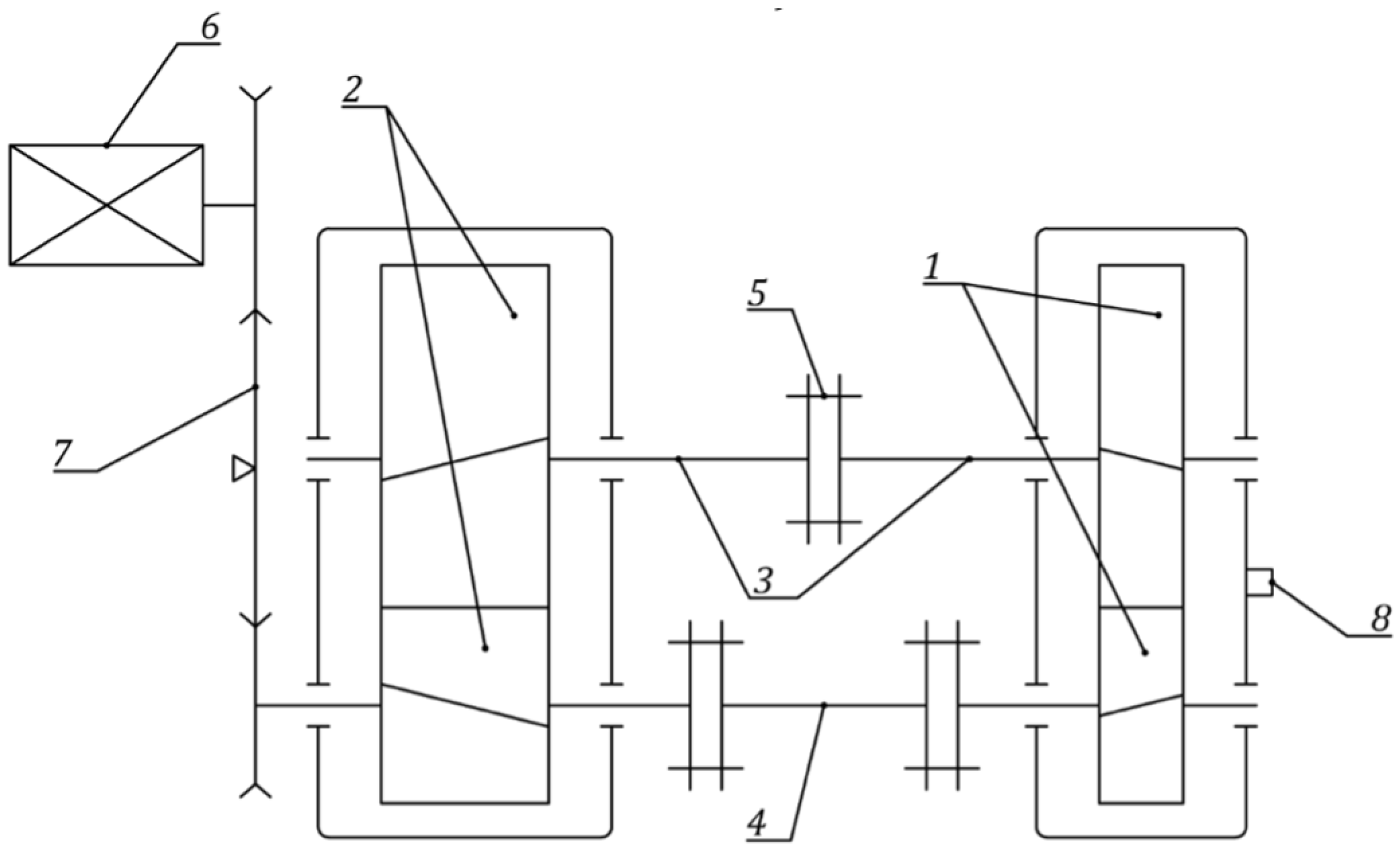
The study was conducted using a circulating power test rig (Figure 1), the same as was used in our previous work [21].

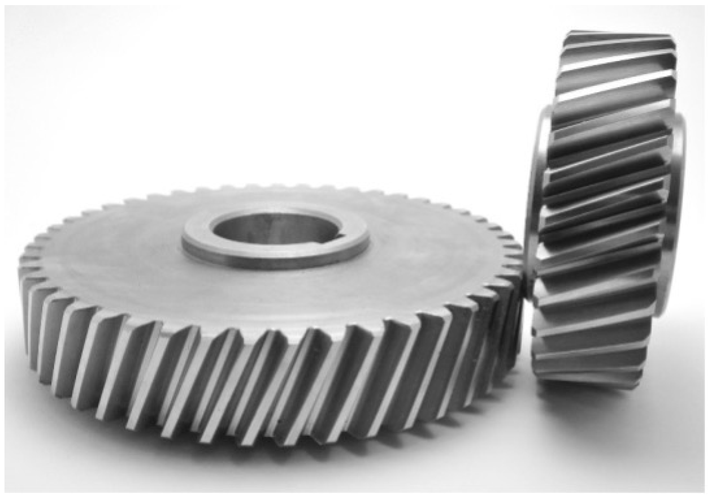
The test rig consists of two gearboxes: the test gearbox (item 1) and the load gearbox (item 2). Both are connected by shafts (items 3 and 4). The initial preload is introduced via a coupling (item 5). An electric motor (item 6), through a belt drive (item 7), provides rotational speed and compensates only for efficiency losses. The load gearbox is specifically designed to withstand all fatigue test cycles. During testing, vibrations of the test gearbox housing were measured in a plane perpendicular to the shaft axis using a piezoelectric accelerometer (item 8). The gears were manufactured on a hobbing machine from 42CrMo4 steel (Figure 2).

Two gear pairs were tested. The first was gas-nitrided (surface hardness: 600–750 HV), while the second remained in a heat-treated condition (hardness: 28–30 HRC). The parameters of the tested gear pairs are summarized in

Table 1. Parameters of the tested gear pairs.

Parameter	Pinion	Gear
Normal module, mm	3	3
Number of teeth	30	47
Face width, mm	30	30
Helix angle, ∘	22.482	22.482
Normal pressure angle, ∘	20	20
Profile shift	0	0
Center distance, mm	125	125
Pitch diameter, mm	97.40	152.59
Tip diameter, mm	103.40	158.59
Root diameter, mm	89.90	145.09

.

The first gear pair (heat-treated and nitrided) was used to train neural networks, as it operated under nominal conditions and did not exhibit damage. The second gearbox (only heat-treated) was employed to evaluate the effectiveness of the developed surface fatigue diagnostic methods.

Table 2. Load stages for the tested gear pairs for gear pair I (quenched and tempered + gas nitriding).

Load Stage	Torque on Pinion [Nm]	Pinion Speed [rpm]	Load Cycles	Cycle Duration
0	42	2500	$1.5\times {10}^5$	1 h
1–8	455	2500	$1.5\times {10}^6$ (per stage)	10 h (per stage)

and

Table 3. Load stages for the tested gear pairs for gear pair II (quenched and tempered only).

Load Stage	Torque on Pinion [Nm]	Pinion Speed [rpm]	Load Cycles	Cycle Duration
0	42	2500	$1.5\times {10}^5$	1 h
1	138	2500	$2.5\times {10}^6$	16 h 40 min
2	244	2500	$2.5\times {10}^6$	16 h 40 min
3	342	2500	$2.5\times {10}^6$	16 h 40 min
4–5	455	2500	$2.5\times {10}^6$ (per stage)	16 h 40 min (per stage)

present the loading conditions for both gear pairs.

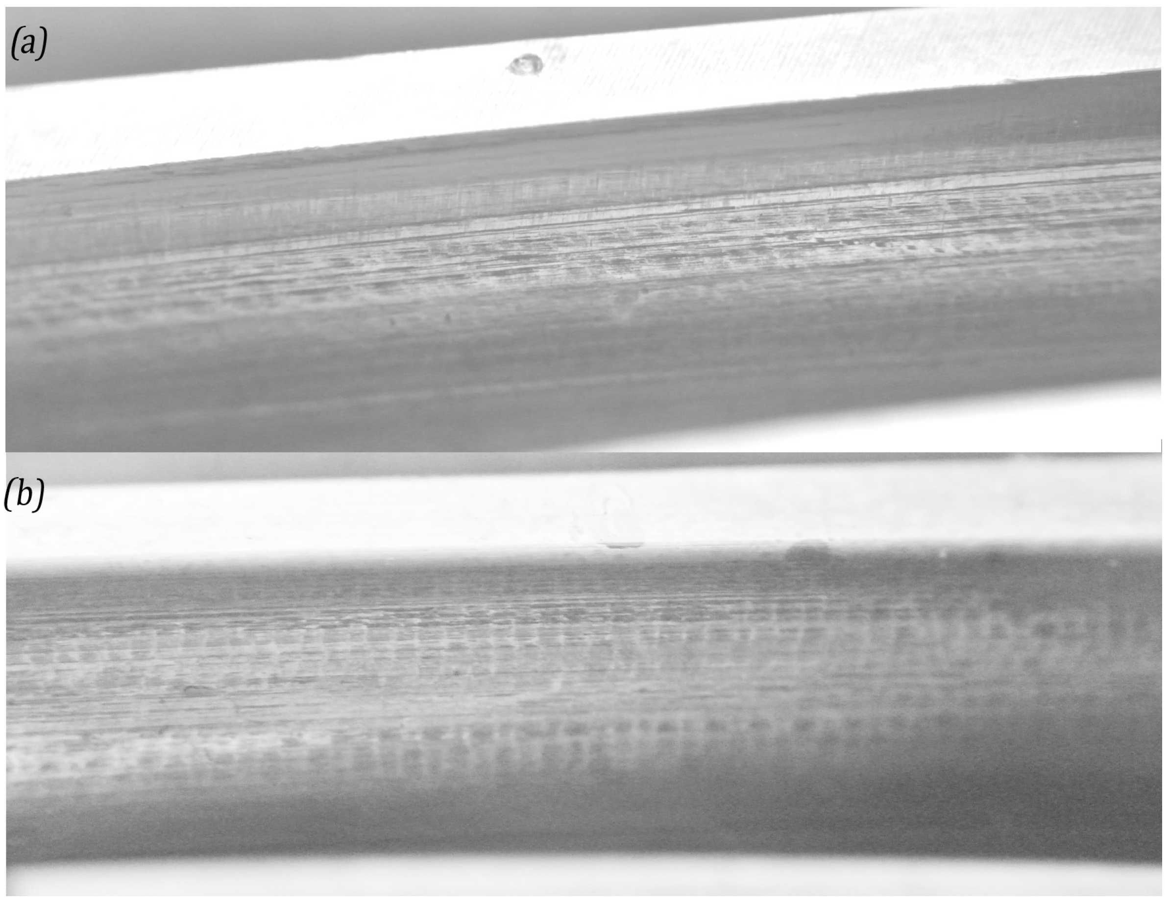
In this study, gear tooth damage was assessed using a method based on image processing of tooth flank surfaces, as in [21]. As previously mentioned, the first gear pair exhibited no signs of damage. Macrophotographs of the tooth surfaces after testing are shown in Figure 3.

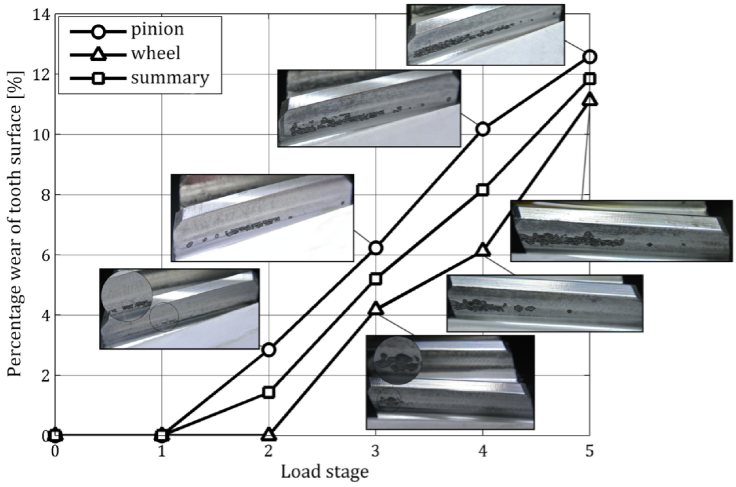
In the case of the second gear pair (heat-treated only), surface fatigue damage in the form of pitting was observed (Figure 4).

2.2. Data Pre-Processing

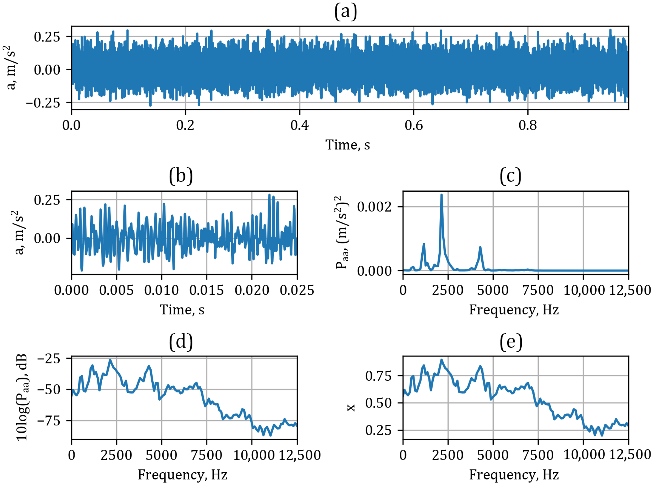
Prior to training the models, the acquired vibration signals from the gearbox housing were appropriately preprocessed. First, the collected vibration signal (Figure 5a) was divided into 25 segments (Figure 5b).

Next, each signal segment was transformed into the frequency domain using Welch’s method of power spectral density (PSD) estimation [22] with a Hann window (Figure 5c). The resulting spectrum was then converted to a logarithmic scale using 10log(PSD) (Figure 5d), and subsequently normalized (x—Figure 5e). This procedure, repeated for all measurements, resulted in 880 normalized periodograms for normal operating conditions (gear pair i) and 560 for the faulty gearbox condition (pitting in gear pair II). 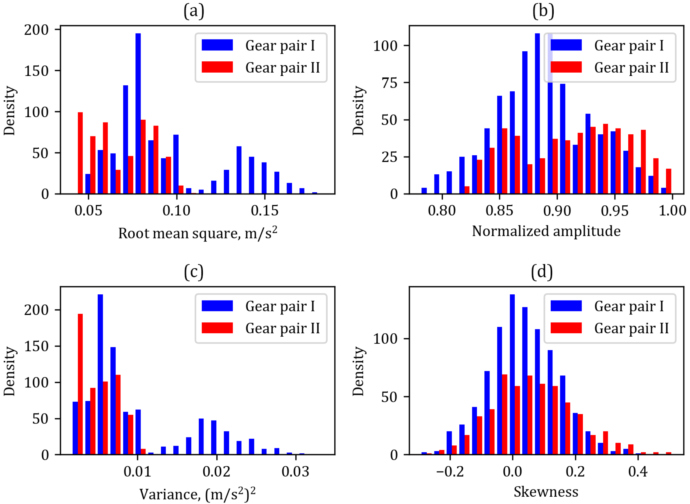Figure 6 shows the distribution of selected parameters of the vibration signals for both classes.

An analysis of the parameter distributions for both classes reveals that they do not provide clear, definitive information about the gearbox operating condition. Therefore, it is essential to employ machine learning methods capable of identifying connections that standard methods may overlook. As input to the machine learning models, we use normalized periodograms, with each periodogram divided into 129 frequency channels.

To summarize, we have a total of 880 periodograms representing normal operating conditions (gear pair i), which are used for model training. The faulty dataset (gear pair II) comprises 560 periodograms. For the purpose of machine learning, the healthy data is split into two subsets: a training set, comprising 80% of the original data; and a test set, comprising the remaining 20%. The faulty data is not used in the training of any algorithms; it is reserved exclusively for verification purposes.

2.3. Machine Learning Methods of Anomaly Detection

Autoencoders are a family of neural networks that are designed to reconstruct their input at the output. While this might seem trivial at first glance, a network with several layers must learn the underlying patterns of the data to accurately obtain the input at the end. Usually, the inner layers of autoencoders are smaller than the input/output layer. Therefore, the initial signal is compressed with each layer, down to the middle layer—called the latent layer. An autoencoder consists of two parts: the encoder, which transforms the input to the latent, the most compressed, representation; and the decoder, which reconstructs the input from the compressed signal. The ideal autoencoder should provide lossless compression of the signal, perfectly learning the mathematical structure of the signals in the training set.

One of the most prominent applications of autoencoders is their usage in signal denoising. This applies to one-dimensional time series as well as images and videos, with the generation of images by subsequent denoising of randomly generated images having recently been shown [23]. However, among their many features, in the aspect of mechanical engineering we are mainly interested in two of them: nonlinear reducing capabilities and sensitivity to anomalous input. As we mentioned, encoders provide a compression method to the data. This serves as a great alternative to conventional statistical dimensional reduction methods, providing a nonlinear reduction of a complicated input. In such a case, the reduced representation can be processed with various machine learning methods, either supervised or non-supervised. The application of this approach to gear fault detection was explored in our previous work [21], where we showed a separation of points representing a healthy and dysfunctional operation. We applied various discrimination techniques to identify the boundary of malfunction.

However, in this work we concentrate on the latter feature of autoencoders, the sensitivity to anomalies. The key idea of the approach is understanding the imbalance between two classes of observations we are interested in. Usually, data on normal operation are much more abundant compared to those on anomalies and failures. Therefore, if the model is trained only on the healthy data, and then if it is given an anomalous record, the reconstruction error, e.g., mean squared error (MSE) between the input and the output of the network, but it could be any other specialized measure, should be distinguishably larger. The weak side of this approach is the accuracy of the model itself. If the autoencoder’s compression loss is too big it becomes hard to distinguish the healthy and faulty reconstructions. To eliminate such situations, one has to provide both an adequate autoencoder architecture and the training that minimizes the spread of distribution of reconstruction error. In the following subsections we describe three different architectures that were used to solve the problem. These are autoencoders based on a densely connected (or fully connected) network, convolutional neural networks, and recurrent neural networks. In this study, we implemented those models using the Keras [24] library.

Each model underwent a similar training and manual hyperparameter tuning procedure. During this process, we considered the following elements:

• Number of layers;
• Size of hidden layers;
• Activation functions.

The results of the experiments were managed using an experimentation control tool, which allowed us to select the best combinations from numerous trials. The final choice was based not only on achieving the lowest loss on the test set but also, more importantly, on minimizing overfitting. Overfitting can be particularly problematic with overly complex models when there is insufficient training data.

As an illustrative example of the experimentation process, we describe the hyperparameter tuning of a convolutional autoencoder, specifically focusing on the number of filters in the convolutional layers. The quantitative results of this search are presented in

Table 4. Fine-tuning hyperparameters using the example of a convolutional autoencoder involved testing several combinations of convolutional filters during an initial training phase of 500 epochs. The numbers in the Model Layers column correspond to the convolutional filters in the encoder, with the decoder constructed as a mirror reflection of the encoder. The remaining columns display the loss function values for both ReLU and ELU activation functions, for the training and test sets, respectively.

Model Layers	ELU — Train Loss	ELU — Test Loss	ReLU — Train Loss	ReLU — Test Loss
16, 8, 8	0.0013	0.0014	0.0014	0.0015
32, 16, 16	0.0012	0.0013	0.0012	0.0013
64, 32, 16	0.0012	0.0014	0.0013	0.0014
128, 64, 32	0.0011	0.0015	0.0009	0.0014

.

For the autoencoder architecture, which consists of three convolutional blocks in the encoder and a mirrored structure in the decoder, we tested various combinations of filter numbers and activation functions. Each configuration was trained for 500 epochs using the Adamax optimizer with a learning rate of ${10}^{-3}$. For each record, we evaluated two activation functions: rectified linear unit (ReLU) and exponential linear unit (ELU).

Our findings indicate that increasing the number of filters, and consequently the number of parameters, generally improved the model’s convergence speed. However, it also led to an increase in overfitting, particularly in configurations with higher filter counts, such as the combination of 128, 64, and 32 filters. This trade-off between convergence speed and overfitting is critical to consider when selecting the optimal hyperparameters for the model.

Given the limited number of experimentally acquired data points (880, divided between training and testing subsets), it was necessary to use a simpler model to mitigate the risk of overfitting, which could otherwise result in poor performance in distinguishing between normal operation and faulty gear pairs. It is important to note that gear wear under production operating conditions occurs gradually. Therefore, it is crucial for the model to accurately capture the features of a healthy gear pair and detect subsequent gear wear that could lead to significant malfunctions.

3. Results

3.1. Fully Connected Autoencoder

The standard autoencoder consists of fully connected layers, which can be mathematically described as

$$y_i=f\left(\sum _j{w}_{ij}{x}_j+b_i\right)$$

(1)

where $x_i$ is the input, $y_i$ is the output, and $w_{ij}$ and $b_i$ are components of the weight matrix and bias vector, respectively. Both weights and biases are trainable parameters that are optimized during the training of the model. The nonlinearity is introduced to the network by the activation function f. A variety of functions are used in the literature, with rectified linear unit (ReLU) $\mathrm{ReLU}\left(x\right)=max\left(0,x\right)$ and its variations being the most popular.

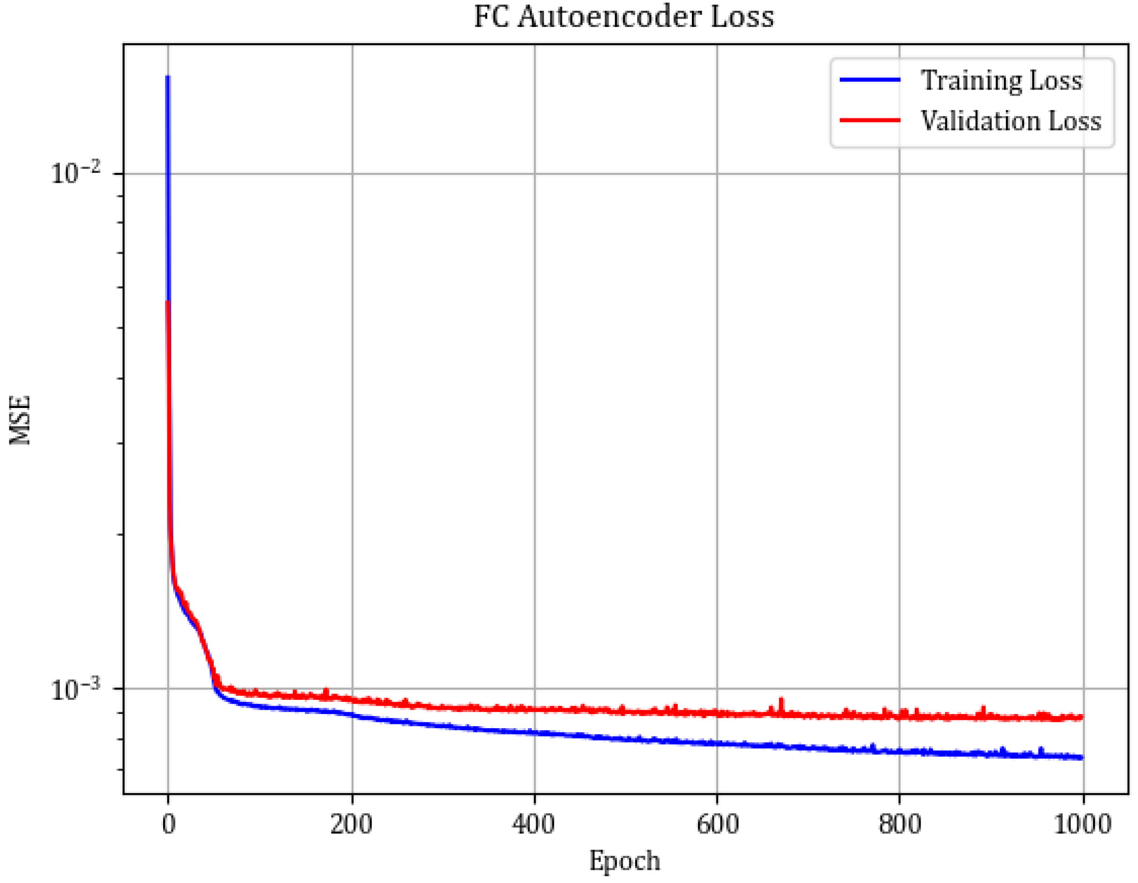
The considered network consists of seven layers in total. The input layer, of size 129, is followed by fully connected layers reducing the dimensions to 64, 32, and 16, which is the latent layer size. The decoder then reverses the process with fully connected layers with 32, 64, and 129 neurons, respectively. For all layers, we apply the ReLU activation function. The network was trained for around 1000 epochs before the early stopping procedure was implemented due to a lack of improvement. Figure 7 shows the example reconstruction of the healthy and damaged gearboxes. The progress of the training is visualized in Figure 8. One can notice slight overfitting with the train set (MSE = $0.0007$), while for the test set MSE = $0.0009$. 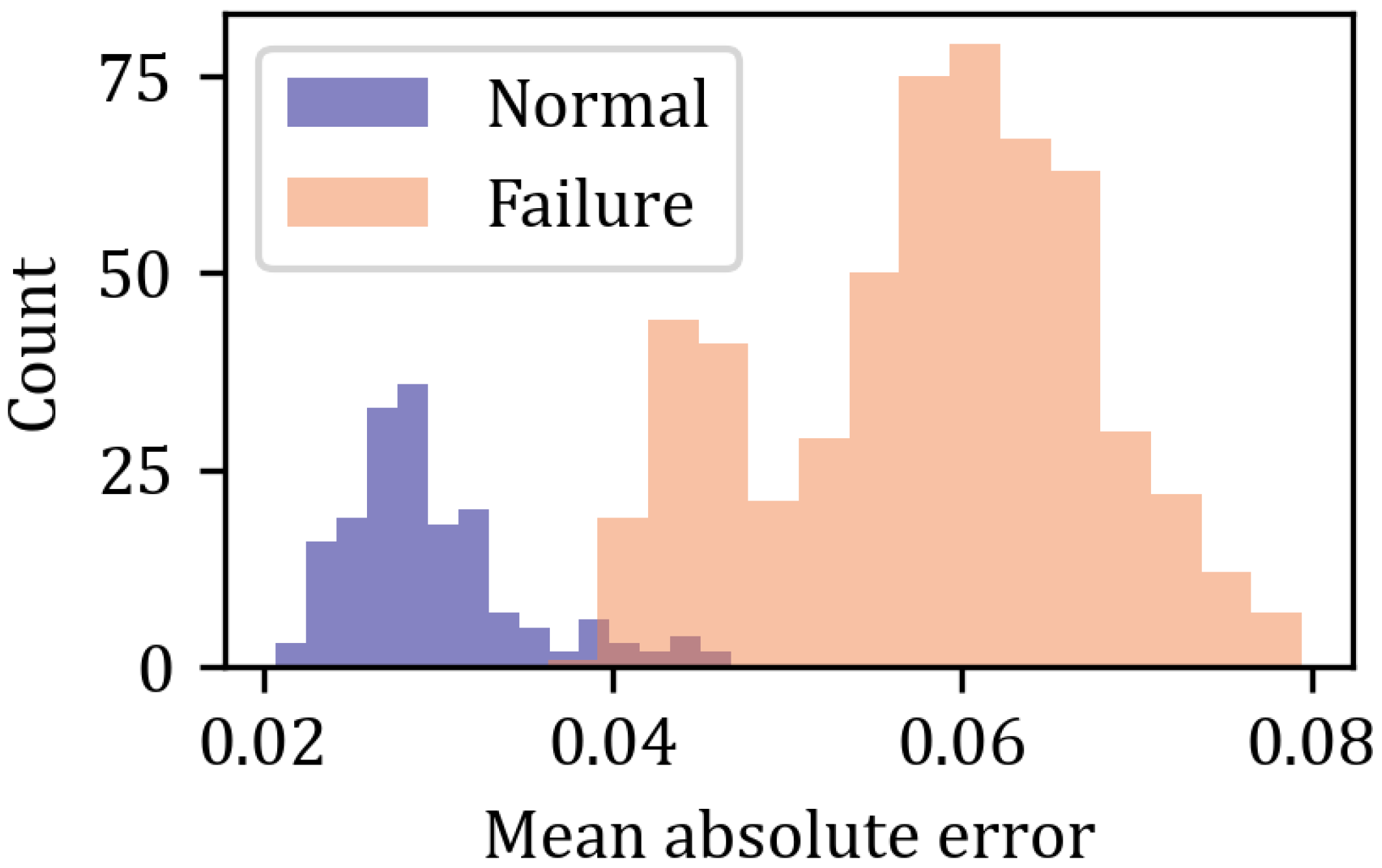In Figure 9 we gather the distributions of mean absolute error (MAE) for normal and failing gearboxes.

3.2. Convolutional Autoencoder

Convolutional layers are highly efficient at recognizing objects in images, as well as patterns in signals in the one-dimensional case. Instead of operating on the entire input, a discrete convolution operation is performed using a kernel, also called a filter. The equation for a one-dimensional convolutional layer is as follows:

$$y_i=\sum _n^l{x}_{i+n} w_n$$

(2)

where $w_n$ is a one-dimensional filter consisting of trainable parameters. A convolutional layer consists of multiple filters, the number of which is a hyperparameter of the model. Each filter individually is responsible for detecting a different type of pattern in the input data. For a more detailed description of the architecture, see the relevant references in [25].

The network implemented in this study consists initially of three blocks of convolution and max pooling layers, where the final one is the global pooling layer. The pooling layers reduce the shape of the data by half on each pass. Then there are fully connected layers of dimensions 32 and 3, representing the latent encoding of the signal, which completes the encoding.

For decoding, the latent layer is pushed to an eight-neuron fully connected layer and then reshaped to be passed through four blocks of up-sampling and deconvolution layers. After such processing, we end up with output of identical dimensions to the input.

Each convolutional block applies exponential linear unit (ELU) activation, which is linear for positive arguments and exponential for negatives, granting a smooth descent to zero instead of the sharp one observed for the ReLU function. This function was applied due to the better performance during the experimentation phase with different model configurations of hyperparameters. However, the dense layers, including the latent layer, use linear activation (or do not use activation at all, depending on convention).

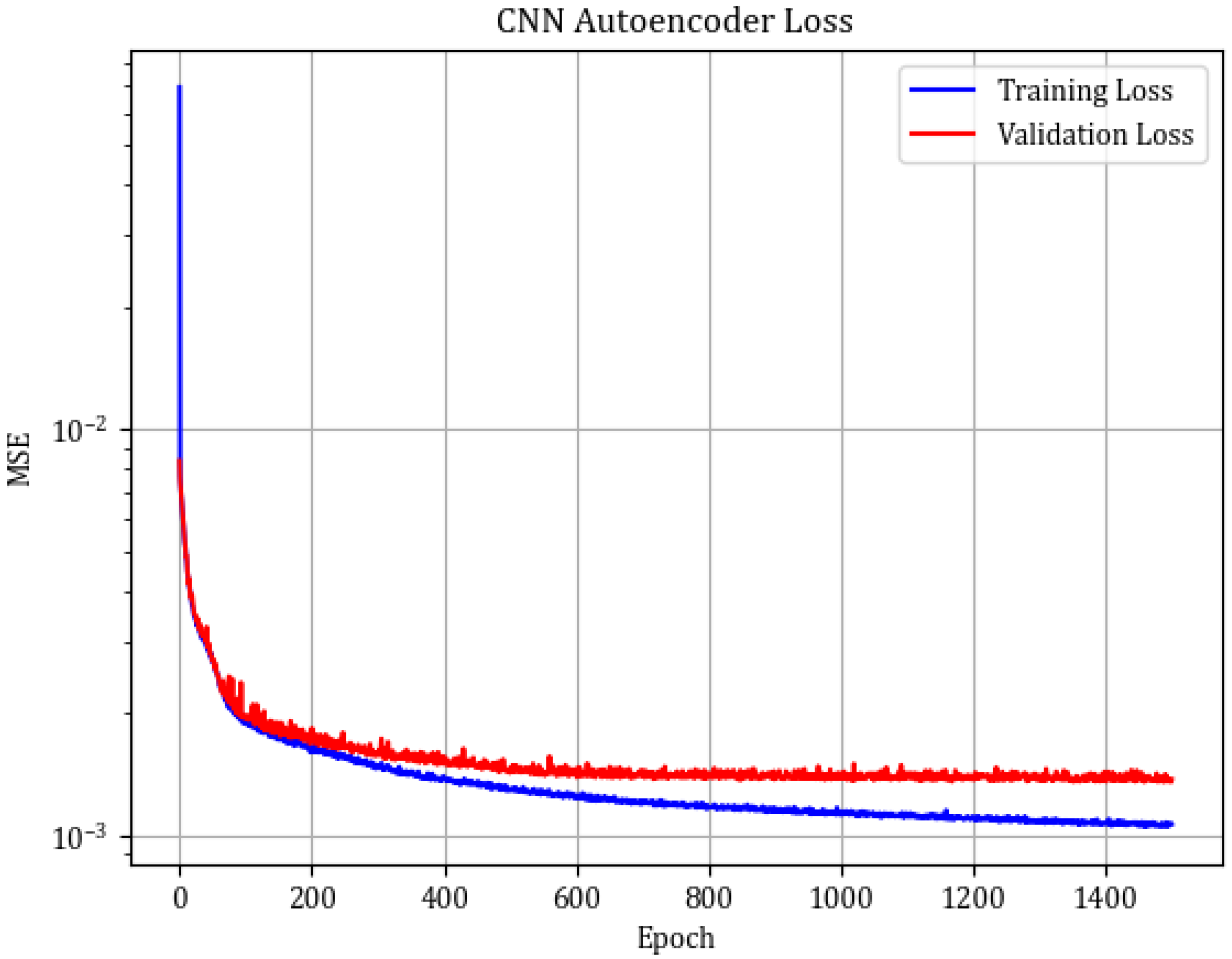
The autoencoder was trained using the Adamax [26] optimizer with a learning rate of ${10}^{-3}$. The total training took 1500 epochs, resulting in an MSE equal to 0.0011 for the train and 0.0014 for the test set, and with MSE = 0.00724 for the faulty gearbox data. Figure 10 shows the example reconstruction of the healthy and damaged gearboxes, while the detailed training history is depicted in Figure 11. In Figure 12 we present the distributions of the MAE for the normal and failing gearboxes.

3.3. Recurrent Autoencoder

The gated recurrent unit (GRU) is an architecture within the domain of recurrent neural networks (RNNs), specifically designed to mitigate the vanishing gradient problem and enhance training efficiency. As delineated in [27], the GRU architecture amalgamates the hidden state and the cell state into a unified state vector, utilizing gating mechanisms to modulate the flow of information. Recurrent layers are optimized for processing of sequential data. They perform exceptionally well in analyses of signals and various time series, where the output is the intertwined result of several time steps of the input sequence with the memory effect on the gates. The components are as follows:

• Reset gate ($r_t$): This gating mechanism determines the extent to which historical information is forgotten. It regulates the contribution of the preceding hidden state to the candidate hidden state.
• Update gate ($z_t$): This gate governs the retention of historical information, functioning analogously to a combined forget and input gate.
• Candidate activation (${\tilde{h}}_t$): This represents the newly computed candidate hidden state, derived through the influence of the reset gate and the current input.
• Hidden state ($h_t$): The final hidden state is computed as a linear interpolation between the preceding hidden state and the candidate hidden state, modulated by the update gate.

Mathematically it can be expressed as follows:

$$\begin{array}{c}\hfill r_j=\sigma \left({\left[W_{r}x\right]}_j+{\left[U_r{h}_{〈t-1〉}\right]}_j\right)\end{array}$$

(3)

$$\begin{array}{c}\hfill z_j=\sigma \left({\left[W_{z}x\right]}_j+{\left[U_z{h}_{〈t-1〉}\right]}_j\right)\end{array}$$

(4)

$$\begin{array}{c}\hfill h_j^{〈t〉}=z_j{h}_j^{〈t-1〉}+\left(1-z_j\right){\tilde{h}}_j^{〈t〉}\end{array}$$

(5)

$$\begin{array}{c}\hfill {\tilde{h}}_j^{〈t〉}=tanh\left({\left[Wx\right]}_j+[U{(r\odot h_{t-1}]}_j\right)\end{array}$$

(6)

where W are adequate weight matrices for the raw input on the r and z gates and U denotes weights for the hidden state.

The autoencoder based on GRU layers, similarly to other autoencoders, compresses the input signal with a GRU layer to a reduced vector. Then, the latent representation is pushed through another recurrent layer, restoring the original signal properties in the output. While the outputs of GRU layers are activated with the standard hyperbolic tangent, for the final layer we use the ReLU function.

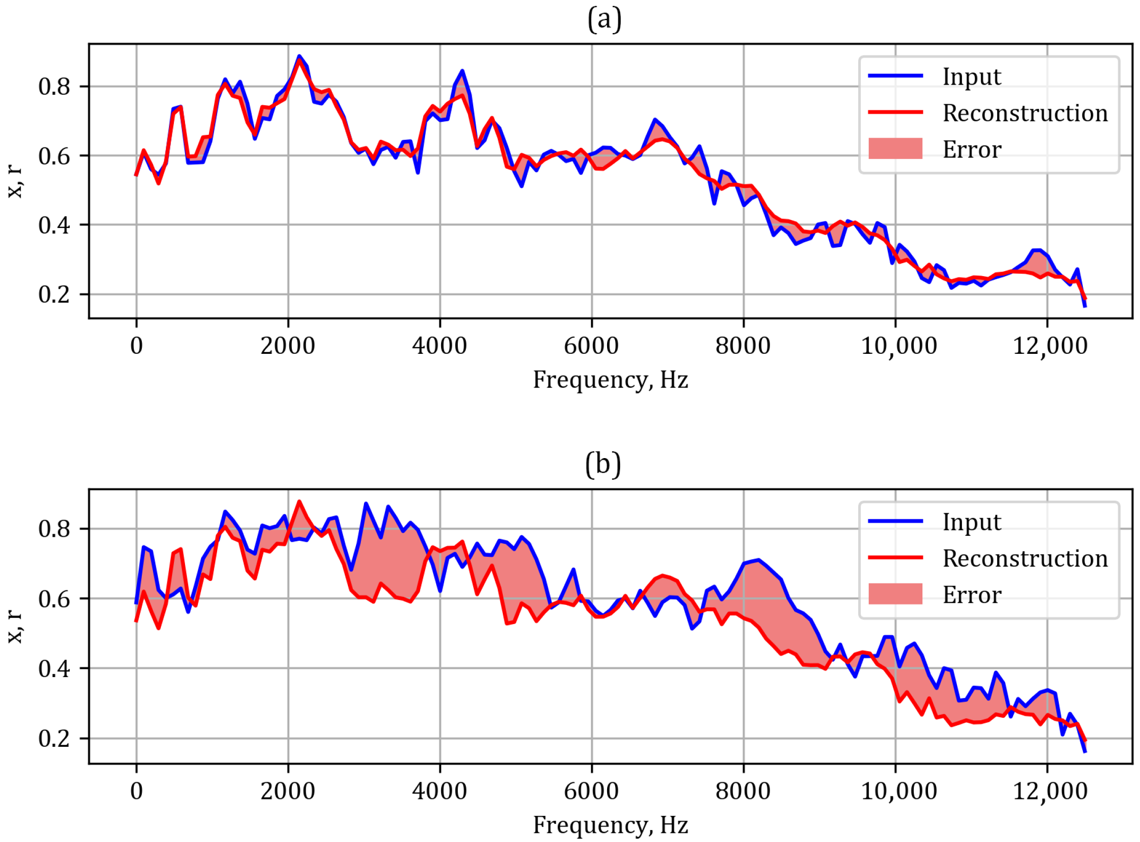
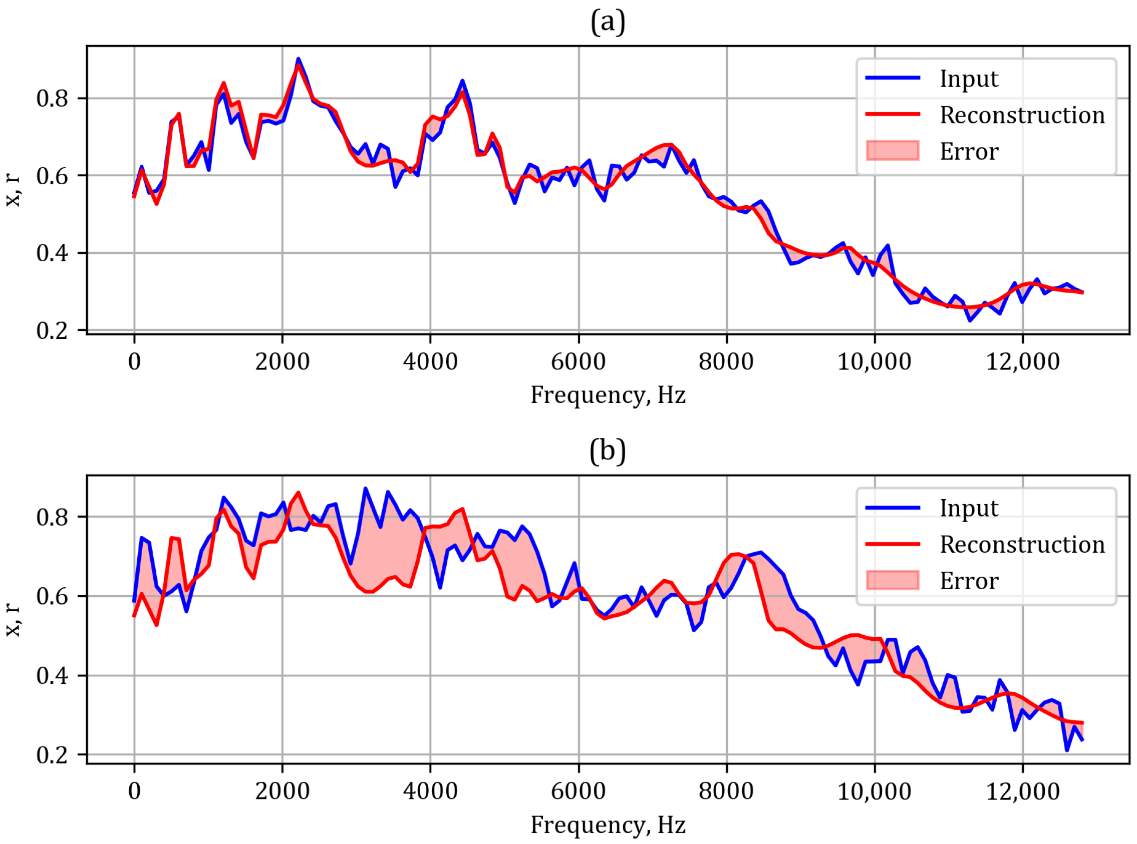
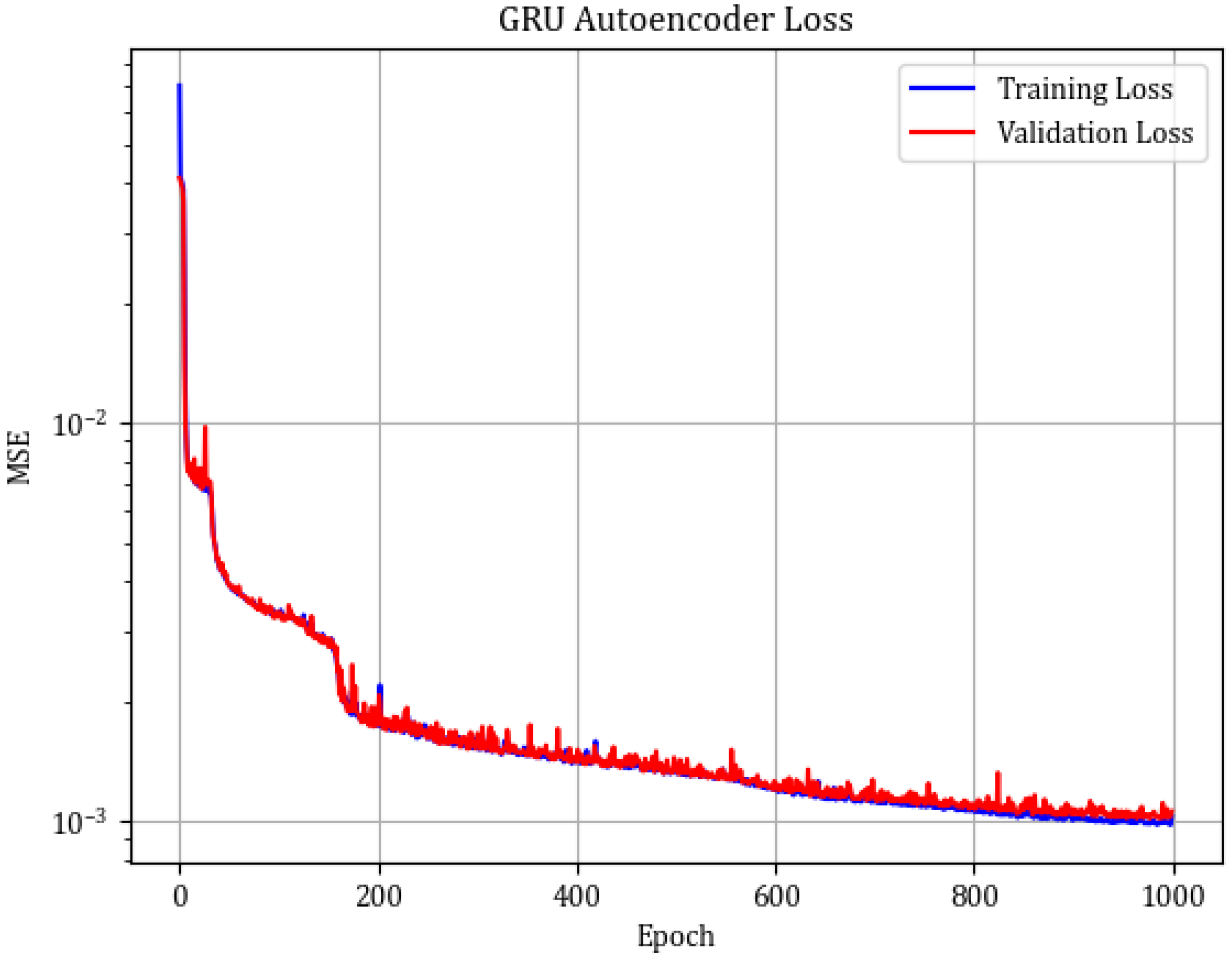
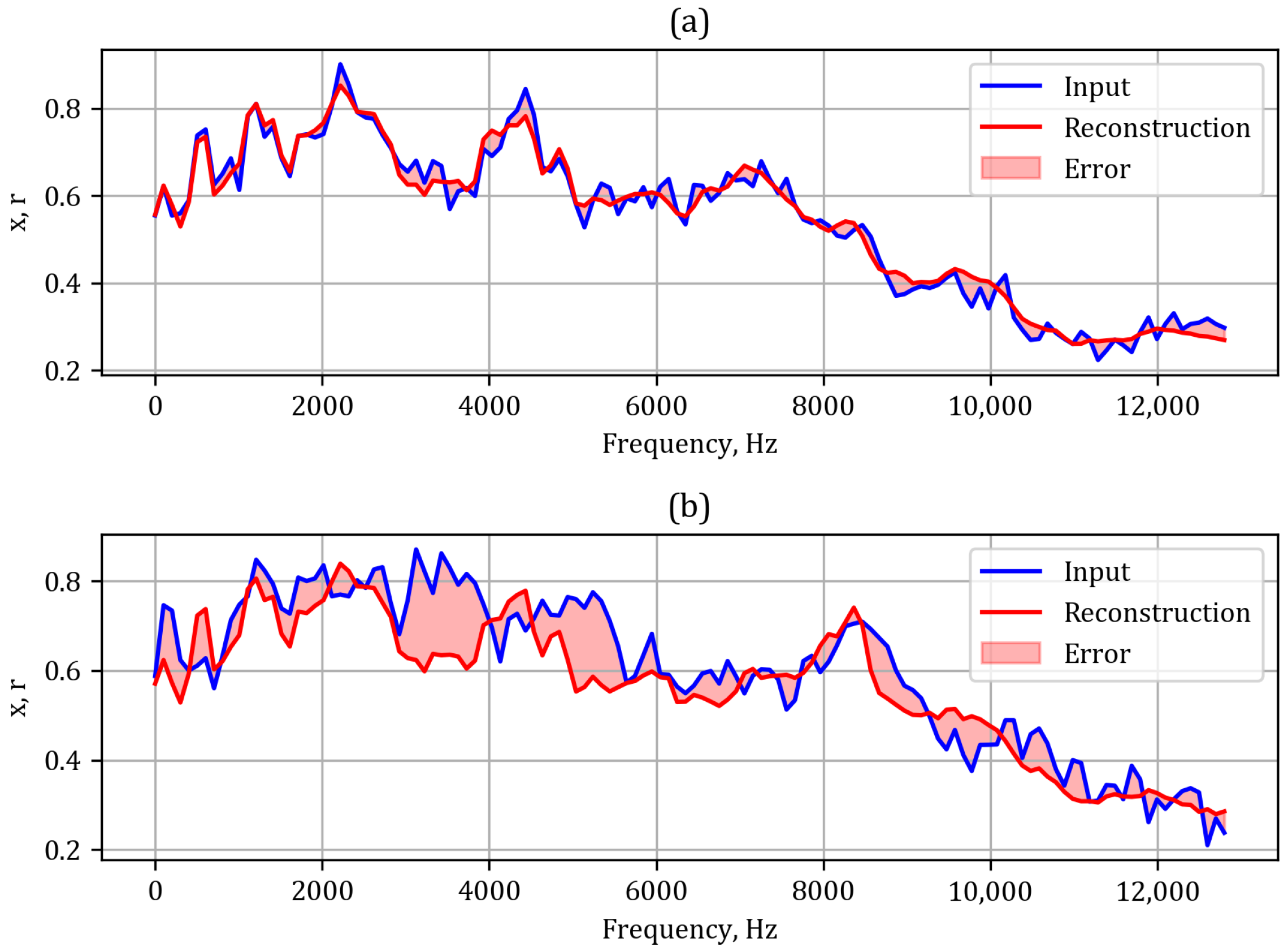
The network was trained using the Adam optimizer with a learning rate of ${10}^{-3}$ and 1000 epochs, resulting in an MSE equal to 0.0010 for the training set and 0.0011 for the test set. However, for the faulty gearbox records the MSE equals 0.0047. In Figure 13 we present an example of a reconstruction for normal operation (Figure 13a) and failure (Figure 13b). One can clearly see the significant difference in the reconstruction error. 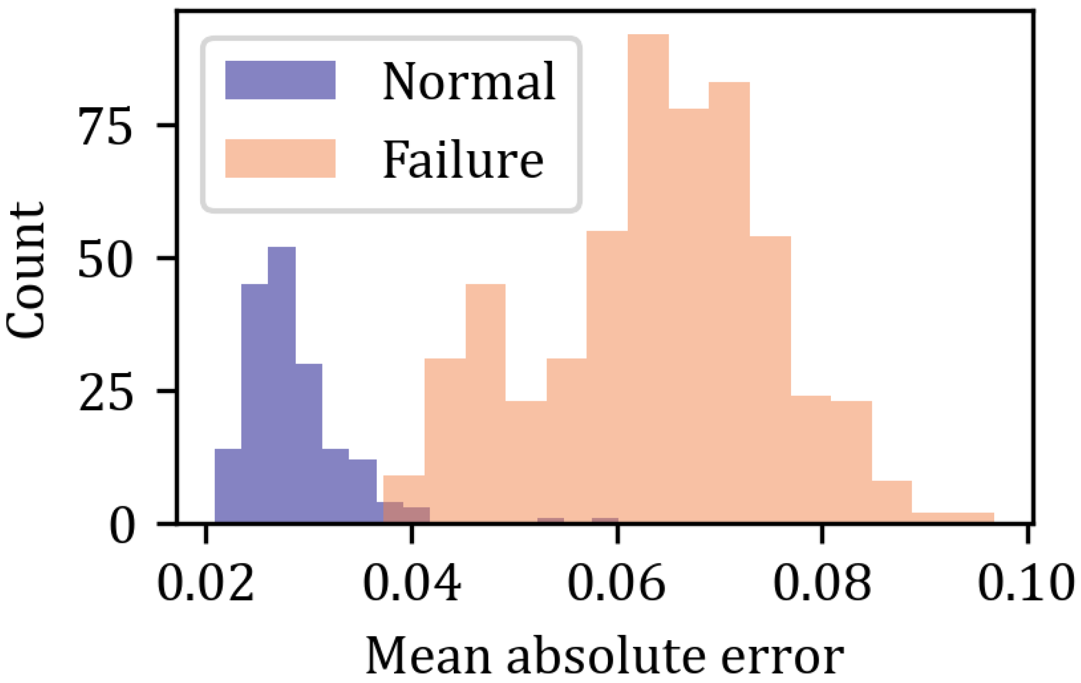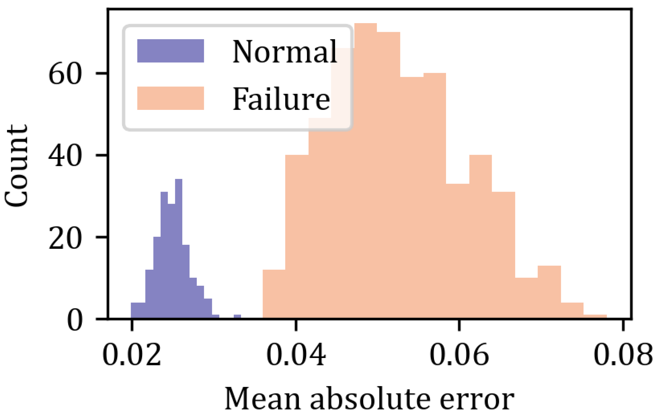The training history is presented in Figure 14. One can clearly notice the better fit of the model compared to the CNN AE. Also the overfitting is significantly smaller. The aggregated errors are presented in a histogram in Figure 15, where the purple and orange shadings correspond to normal and failure records, respectively.

4. Discussion

Each of the three algorithms was trained on the healthy data and provided us with a set of reconstructions of the initial signal for both normal operation and failure of the gear box. In Figure 9, Figure 12, and Figure 15 we present the distributions of the MAE of the reconstruction. However, the problem had to be reformulated in terms of classification, since we are seeking for an answer to whether the machine is operational or broken. The essential question at this point is where one should place the boundary between the records that should be classified as healthy or faulty. The conventional approach defines the threshold in a standard way:

$$t={\mu }_{MAE}+n{\sigma }_{MAE}$$

(7)

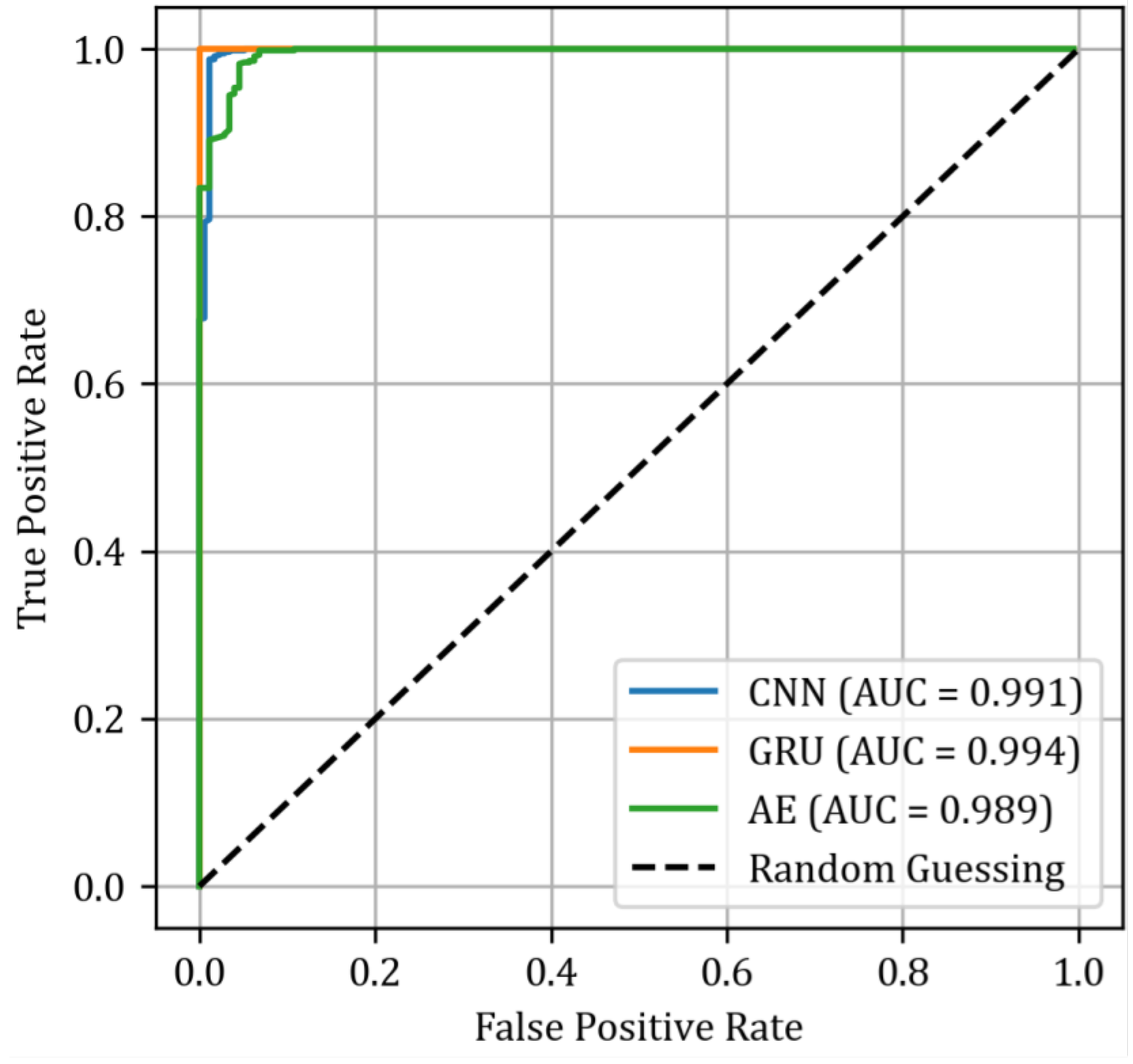
where ${\mu }_{MAE}$ is the average mean absolute error, ${\sigma }_{MAE}$ is the standard deviation of the mean absolute error, and n is an arbitrary positive constant. Both quantities originate from the test set. Then, to compare the performance of classifiers, we can use receiver operating characteristic (ROC) curves (Figure 16).

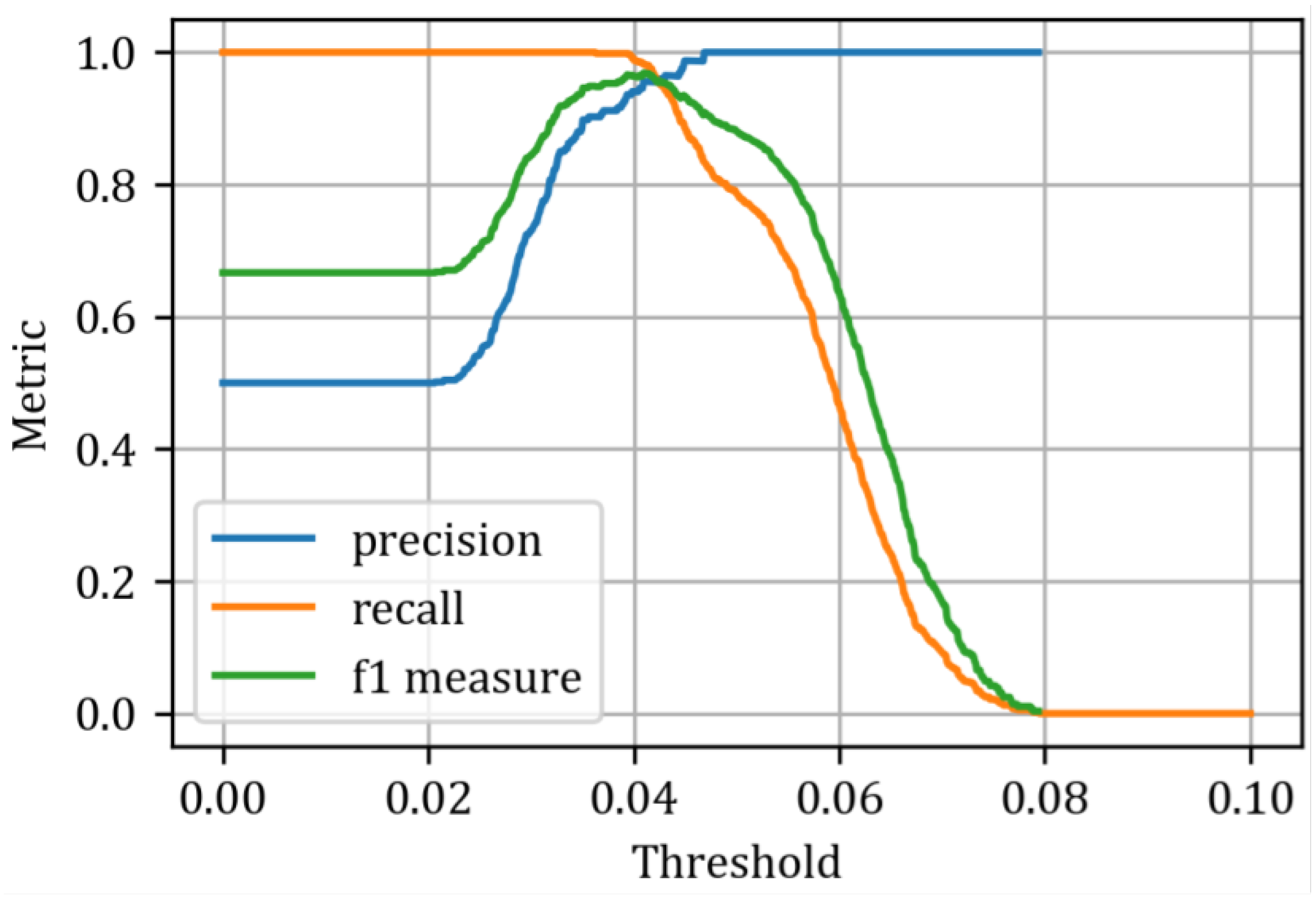
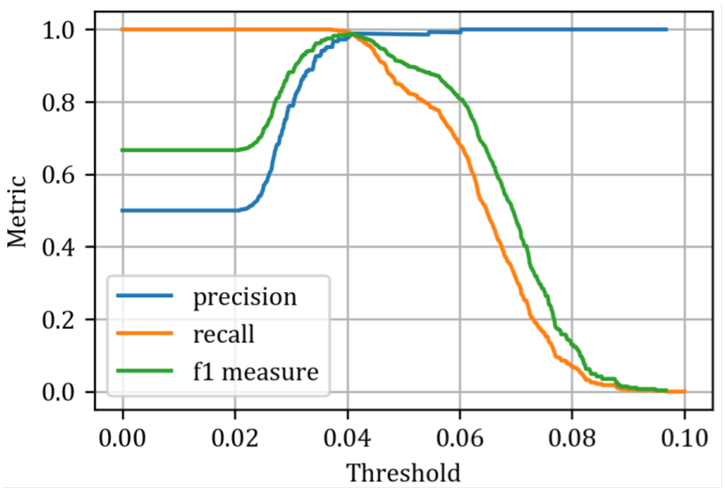
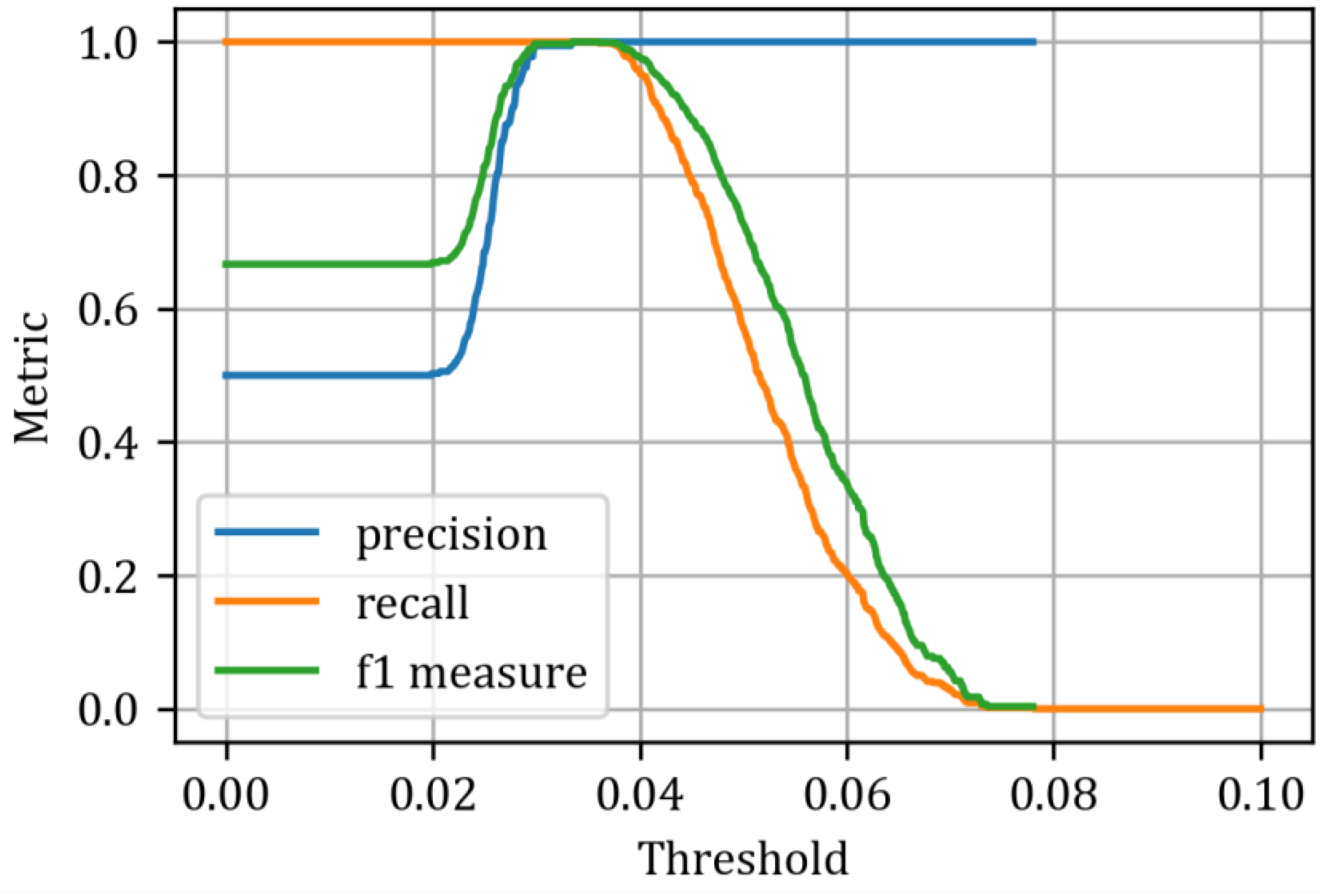
These curves illustrate the relationship between the true positive rate and the false positive rate for various threshold values. One of the key metrics for assessing classification performance is the area under the curve (AUC). In this analysis (Figure 16), it is evident that the best classifier is the recurrent autoencoder, which demonstrates excellent separation of predicted states and serves as an almost ideal classifier, achieving an AUC of 0.994. The other classifiers performed slightly worse, with AUCs of 0.991 for the convolutional autoencoder and 0.989 for the feedforward autoencoder, respectively. To determine the optimal threshold values, we can use metrics such as precision, recall, and the F1 measure, which are calculated for various threshold values, as illustrated in Figure 17, Figure 18 and Figure 19.

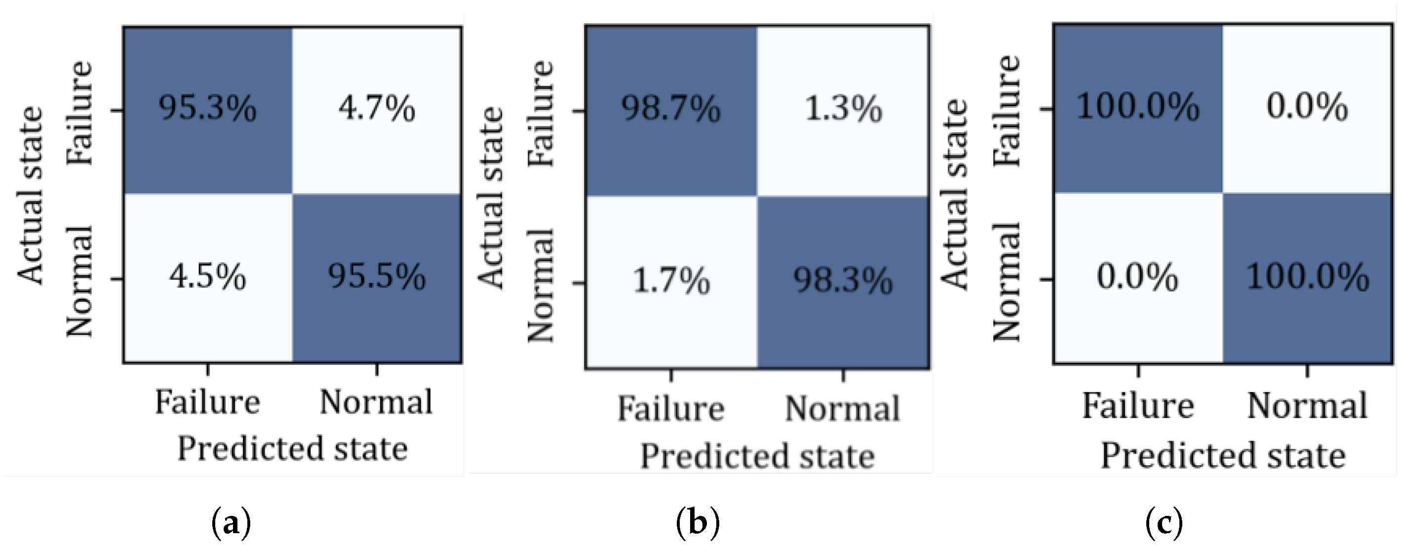
These curves are helpful for selecting threshold values, providing insight into the trade-offs between these metrics. In this study, we have chosen the intersection point of the three curves as the optimal threshold value. This results in a threshold of 0.0424 ($n=2.43$) for the fully connected autoencoder, 0.0407 ($n=2.46$) for the convolutional autoencoder, and 0.0347 ($n=4.63$) for the recurrent autoencoder. The classification results are presented in

Table 5. Classification results.

Model	Threshold	Precision	Recall	F1-Score
Fully Connected AE	0.0424	0.9545	0.9535	0.9540
Convolutional AE	0.0407	0.9830	0.9875	0.9852
Recurrent (GRU) AE	0.0347	1.0	1.0	1.0

and Figure 20.

5. Conclusions

In this paper, we explored three different neural network architectures for building an autoencoder capable of the most accurate anomaly detection for our self-designed and experimentally measured operating gears. One might question why more advanced techniques, such as transformers, known for their exceptional performance, were not employed. The explanation lies in the number of data points available. This study relies solely on experimentally gathered data, thereby constraining the complexity of the models and the number of their parameters to the available dataset size. The chosen architectures represent an optimal balance between complexity and dataset size. Nonetheless, given the results obtained, these architectures have proven to be sufficiently effective.

Starting with the fully connected network, we found an overall good performance, yet it was far from perfect. Then, by applying one-dimensional convolutional layers to our problem, we intended to find patterns in the periodogram that would be easily detected by this architecture. This approach proved successful, as we obtained a noticeable improvement in model performance. Finally, we applied a recurrent neural network architecture, based on GRU cells, which were originally designed to work with time series and sequences, both in signals and natural language processing. While the original intention of these networks was somewhat different, given that our periodogram is a function of frequency rather than time, their performance was spectacular. Another crucial aspect was fine-tuning the threshold used to translate the autoencoder’s output into classification. For the optimal threshold, we selected the value at the intersection point of the recall and precision curves. While for the fully connected AE this value is around 2.5 standard deviations, and similar for the CNN, it is particularly interesting to note that the threshold for the GRU AEs significantly exceeds the standard triple multiplicity of standard deviation, corresponding to a 99.7% confidence interval. This ensures that these methods, especially the GRU AE, are robust against false alarms and capable of detecting the actual wear of the gearbox that will lead to imminent failure. In conclusion, our study demonstrates the effectiveness of advanced neural network architectures in enhancing anomaly detection for operating gears. The GRU-based autoencoder, in particular, stands out for its robustness and accuracy, significantly reducing the likelihood of false alarms while reliably identifying critical anomalies. This is particularly important in areas such as wind turbine gearboxes, where false alarms can be very costly. These findings not only highlight the potential of neural networks in predictive maintenance but also pave the way for further research into optimizing and applying these models in various industrial contexts. Future work will focus on real-time implementation and further validation of these models under diverse operating conditions to ensure their reliability and scalability.

The proposed approach, while developed and validated under controlled laboratory conditions, provides a robust foundation for broader application. Notably, the autoencoder models can be fine-tuned using small amounts of vibration data collected from gear systems of various sizes, shapes, or operating environments. This transfer learning strategy enhances the models’ ability to generalize and adapt to real-world variations, which can include environmental noise, load dynamics, and system-specific resonance effects that may distort sensor signals even in healthy states. As a result, the methodology is not limited to the specific gearbox used in the study; rather, it offers a flexible framework that can be adapted to different gear transmission systems through targeted re-training or domain adaptation. Future work will focus on testing this adaptability in real-world conditions and evaluating performance across various gear geometries and environmental scenarios.