A Novel Renewable Energy Scenario Generation Method Based on Multi-Resolution Denoising Diffusion Probabilistic Models

Abstract

As the global energy system accelerates its transition toward a low-carbon economy, renewable energy sources (RESs), such as wind and photovoltaic power, are rapidly replacing traditional fossil fuels. These RESs are becoming a critical element of deeply decarbonized power systems (DDPSs). However, the inherent non-stationarity, multi-scale volatility, and uncontrollability of RES output significantly increase the risk of source–load imbalance, posing serious challenges to the reliability and economic efficiency of power systems. Scenario generation technology has emerged as a critical tool to quantify uncertainty and support dispatch optimization. Nevertheless, conventional scenario generation methods often fail to produce highly credible wind and solar output scenarios. To address this gap, this paper proposes a novel renewable energy scenario generation method based on a multi-resolution diffusion model. To accurately capture fluctuation characteristics across multiple time scales, we introduce a diffusion model in conjunction with a multi-scale time series decomposition approach, forming a multi-stage diffusion modeling framework capable of representing both long-term trends and short-term fluctuations in RES output. A cascaded conditional diffusion modeling framework is designed, leveraging historical trend information as a conditioning input to enhance the physical consistency of generated scenarios. Furthermore, a forecast-guided fusion strategy is proposed to jointly model long-term and short-term dynamics, thereby improving the generalization capability of long-term scenario generation. Simulation results demonstrate that MDDPM achieves a Wasserstein Distance (WD) of 0.0156 in the wind power scenario, outperforming DDPM (WD = 0.0185) and MC (WD = 0.0305). Additionally, MDDPM improves the Global Coverage Rate (GCR) by 15% compared to MC and other baselines.

1. Introduction

The global shift towards mitigating energy imbalances and climate change has accelerated the development of distributed energy systems, with RESs such as wind and solar power replacing traditional fossil fuels [1]. However, the intermittent nature of RESs presents significant challenges for power systems, affecting both their reliability and economic performance [2]. As RES penetration increases, so does the uncertainty in power generation, demanding more accurate probabilistic models for operational and planning decisions. These decisions are driven by stochastic optimization frameworks reliant on representative scenario sets to capture RES uncertainties [3].

Scenario generation replicates the real-world variability of RES outputs through stochastic models that generate synthetic time series data. These models incorporate both historical patterns and future uncertainties. In addition to RES, scenario generation techniques have applications in domains like transportation and smart grid management. Chen et al. [4] proposed a deep reinforcement learning-based energy management strategy, and Gao et al. [5] designed a three-stage framework for cophasing power systems with hybrid storage, relying on scenario generation to handle uncertainties and improve scheduling. Existing scenario generation methods are typically parametric [6], non-parametric, or deep generative models [7].

Scenario generation based on parametric models assumes that uncertainty in RESs follows a predefined probability distribution, with parameters estimated using historical data [8]. This two-stage method first defines the uncertainty distribution and then generates scenarios using techniques like Monte Carlo (MC) sampling and Latin hypercube sampling [9]. Díaz G et al. [10] developed a wind farm output generation framework using a state-space model, integrating Kalman filtering with a Box–Jenkins model for performance simulation. Zhou R et al. [11] introduced a probabilistic spatiotemporal method for dynamic optimal power flow analysis, balancing computational complexity and precision with Latin hypercube and copula importance sampling. Guimarães I O et al. [12] proposed a quasi-sequential MC simulation method for evaluating distributed generation system reliability. While parametric models are efficient, their reliance on artificial distributions can compromise scenario quality, leading to issues such as overfitting, limited generalization, and sensitivity to parameter choices.

Non-parametric methods have gained increasing attention due to their ability to capture the nonlinear and dynamic characteristics of RES generation without relying on fixed distributional assumptions [13]. These techniques, including moment matching and distance matching, generate scenarios by minimizing discrepancies between generated and target statistical attributes. Li J. et al. [14] developed a moment-matching method to generate wind power scenarios that reflect its inherent stochasticity, while Li B. et al. [15] proposed a data clustering approach that improves scenario quality by grouping wind farms based on their correlation structure. Despite these advancements, non-parametric approaches may overlook low-probability, high-impact scenarios, limiting their practical use in complex operational environments. To address these limitations, machine learning techniques have been introduced. Vagropoulos S. I. et al. [16] applied artificial neural networks to model short-term stochastic scheduling, incorporating cross-variable correlations and scenario reduction techniques. Their method was validated with data from Crete and mainland Greece. Wang H. et al. [17] used neural networks to model wind power stochastic processes and ramp event probabilities, though their reliance on feature selection limits generalization and reliability.

The rapid development of artificial intelligence has led to significant advancements in deep generative models for scenario generation, including Variational Autoencoders (VAEs) [18], Normalizing Flows (NFs) [19], and Generative Adversarial Networks (GANs) [20]. Li et al. [21] integrated external meteorological features and internal latent variables into a VAE-GAN framework, employing mutual information maximization to improve controllability and the capability to generate extreme scenarios. However, GAN-based approaches still face notable challenges, including mode collapse, poor temporal consistency, and limited ability to incorporate historical context, making it difficult to model short-term variability and non-stationarity in renewable generation data.

Denoising Diffusion Probabilistic Models (DDPMs) are generative models that add noise to data and reverse the process to recover clean data, making them ideal for modeling both long-term trends and short-term fluctuations in scenario generation. DDPMs offer a mathematically tractable formulation, ensuring stable training, principled uncertainty quantification, and fine-grained control over the sampling process [22]. Zhao et al. [23] developed a Conditional Diffusion-based Scenario Generation model to address joint source–load uncertainties in DDPSs. Their model incorporates a Conditional Spatio-Temporal Fusion Module to capture spatio-temporal correlations between multi-energy loads, and a Conditional Scenario Noise Estimation Module to enhance the diversity of generated scenarios. Dong et al. [24] proposed a Conditional Latent Diffusion Model for short-term wind power scenario generation, decomposing the task into deterministic forecast regression and error scenario generation. Their method uses Numerical Weather Prediction data and an embedding network for efficient forecasting, followed by a denoising network that generates forecast error scenarios, improving accuracy and reducing diffusion complexity [25,26]. Despite these advances, many DDPM-based methods use a single-scale diffusion process at all temporal levels [27], which overlooks the distinct short-term and long-term features of the output, leading to attenuation of short-term fluctuations and distortion of long-term patterns [28].

Accordingly, this study introduces a novel Multi-resolution Denoising Diffusion Probabilistic Model (MDDPM) for wind–solar power scenario generation. The proposed model incorporates multi-scale time series decomposition, cascaded diffusion modeling, and condition-aware denoising to generate scenarios with physical consistency, statistical controllability, and strong temporal coherence. The core innovations are summarized as follows:

• To effectively capture both long-term trends and short-term fluctuations, we employ a multi-scale decomposition strategy within a multi-stage conditional diffusion framework. Initially, low-frequency components are extracted and diffused to establish global structure. High-frequency details are then recursively denoised and integrated into the diffusion process, ensuring accurate cross-scale sequence reconstruction and dynamic adaptability.
• To ensure physical realism in generated scenarios, a condition-constrained denoising mechanism is implemented through the incorporation of historical and trend-based priors at each stage. In addition, a forecast-guided fusion strategy is employed to strengthen long-range dependency modeling and improve generalization over extended horizons.

To address the limitations of existing scenario generation methods in capturing both long-term and short-term uncertainties of RESs, we propose a Multi-resolution Denoising Diffusion Probabilistic Model (MDDPM). Our method enhances scenario diversity and realism by integrating historical trends and high-resolution forecast signals through a multi-stage diffusion process. In the remainder of this paper, Section 2 introduces the MDDPM framework in detail, including the model architecture, conditional inputs, and optimization strategy. Section 3 describes the experimental design, datasets, and evaluation metrics, followed by a comparative analysis with state-of-the-art baselines. Finally, Section 4 concludes the paper by highlighting key findings, practical implications, and directions for future research.

2. Multi-Resolution Denoising Diffusion Probabilistic Model

The overall architecture of the proposed multi-resolution conditional diffusion model is illustrated in Figure 1. The framework consists of three main components: (1) a multi-scale time series decomposition module, which separates the input historical sequence into low-frequency (trend) and high-frequency (fluctuation) components; (2) a cascaded conditional diffusion module, where the generation of low-frequency scenarios is performed first to establish the global structure, followed by the conditional generation of high-frequency components that refine the fine-scale details; (3) a sequence reconstruction mechanism, which integrates all decomposed components into complete future scenarios. This hierarchical design ensures that the model captures both long-term dependencies and short-term variability in renewable energy outputs, enabling physically consistent and statistically diverse scenario generation. This approach enhances the predictability and physical consistency of wind and solar power output data through time-series decomposition, cascaded diffusion modeling, and a conditional denoising mechanism. In this section, we provide a layer-by-layer introduction to the core components of the proposed framework, including the fundamental theory of diffusion models, the Forecast-Guided Fusion strategy, the reverse denoising process, and the model training methodology.

2.1. Denoising Diffusion Probabilistic Models

DDPMs are a class of generative models that learn to transform data distributions into noise and then reverse the process to reconstruct the original distribution. This approach has shown promise in applications such as image generation [29] and speech synthesis [30], making it well-suited for modeling the complex and uncertain nature of renewable energy generation over time.

The core principle of DDPMs is based on a Markov chain process, where each step in the diffusion process involves the addition of noise to the data. This noisy version of the data is then iteratively reconstructed to approximate its original state via a reverse process. In the forward process, the model systematically adds Gaussian noise to the original data. This noise is gradually increased step by step, based on a predefined schedule, allowing the model to explore a range of possible variations in the data. In the reverse process, the model iteratively removes this noise, effectively reconstructing a plausible energy output scenario that reflects both the observed data distribution and inherent uncertainties:

$$q(x_{1:K}\mid x_0)=\prod _{k=1}^{K}q(x_k\mid x_{k-1})$$

(1)

In the forward modeling of the diffusion process, the conditional probability distribution $q(x_k\mid x_{k-1})$ describes how noise is gradually added to the original data at each step, where ${\beta }_k$ is the noise variance at step k, which lies in the interval $[0,1]$. This process is modeled as a Gaussian distribution:

$$q(x_k\mid x_{k-1})=\mathcal{N}\left(x_k;\sqrt{{\alpha }_k}{x}_{k-1},{\beta }_k\mathbf{I}\right),k=1,\dots ,K.$$

(2)

$${\alpha }_k=1-{\beta }_k$$

(3)

According to the properties of the Gaussian distribution, the relationship between $x_k$ and $x_{k-1}$ can be expressed as follows:

$${\overline{\alpha }}_k=\prod _{s=1}^k{\alpha }_s$$

(4)

$$x_k=\sqrt{{\alpha }_k}{x}_{k-1}+\sqrt{1-{\alpha }_k}ϵ,ϵ\sim \mathcal{N}(0,I)$$

(5)

Here, $ϵ$ denotes the Gaussian noise sampled at time step $k-1$ in the diffusion process.

In DDPMs, the reverse diffusion process is defined as a Markov process. Specifically, in the k-th step of the reverse process, $x_{k-1}$ is obtained by sampling from the following Gaussian distribution:

$$x_{k-1}={\displaystyle \frac{1}{\sqrt{{\alpha }_k}}}\left(x_k-{\displaystyle \frac{1-{\alpha }_k}{\sqrt{1-{\overline{\alpha }}_k}}}{z}_{\theta }(x_k,k)\right)+{\tilde{\beta }}_kϵ$$

(6)

$$p_{\theta }(x_{k-1}\mid x_k)=\mathcal{N}(x_{k-1};{\mu }_{\theta }(x_k,k),{\Sigma }_{\theta }(x_k,k))$$

(7)

Here, s is a small offset parameter, and ${\overline{\alpha }}_k$ represents the cumulative noise retention ratio for the first k steps. This cosine schedule enables the model to retain more original data in early diffusion stages while gradually increasing noise intensity in later steps.

The objective of the reverse process is to estimate $p(x_{k-1}\mid x_k)$, which removes noise and recovers the true data. However, since the explicit form of $p(x_{k-1}\mid x_k)$ is unknown and cannot be directly computed using Bayes’ theorem, it is typically inferred from the previous Gaussian conditional distribution $q(x_{k-1}\mid x_k,x_0)$. According to the Markov property of the diffusion process, we have

$$q(x_{k-1}\mid x_k,x_0)=\mathcal{N}\left(x_{k-1};{\tilde{\mu }}_k(x_k,x_0),{\tilde{\beta }}_k\right)$$

(8)

$${\tilde{\mu }}_k(x_k,x_0)={\displaystyle \frac{1}{\sqrt{{\alpha }_k}}}\left(x_k-{\displaystyle \frac{1-{\alpha }_k}{\sqrt{1-{\overline{\alpha }}_k}}}ϵ\right)$$

(9)

$${\tilde{\beta }}_k={\displaystyle \frac{1-{\overline{\alpha }}_{k-1}}{1-{\overline{\alpha }}_k}}{\beta }_k$$

(10)

Here, $\mu \left(x_k\right)$ denotes the mean predicted by the network, and the loss function L is defined as $L={∥x_0-\mu \left(x_k\right)∥}^2$.

$$x_0={\displaystyle \frac{1}{\sqrt{{\overline{\alpha }}_k}}}\left(x_k-\sqrt{1-{\overline{\alpha }}_k}ϵ\right)$$

(11)

Therefore, $\mu \left(x_k\right)$ can be parameterized as follows:

$$\mu \left(x_k\right)={\displaystyle \frac{1}{\sqrt{{\overline{\alpha }}_k}}}\left(x_k-\sqrt{1-{\overline{\alpha }}_k}{z}_{\theta }(x_k,k)\right)$$

(12)

Here, $x_k$ and k serve as the inputs to the prediction model $z\left(\theta \right)$, while $z_{\theta }(x_k,k)$ is the output. Furthermore, the loss function can be reformulated as follows:

$$L\left(\theta \right)={\mathbb{E}}_{x_0,ϵ,k}\left[{∥ϵ-{ϵ}_{\theta }(x_k,k)∥}^2\right]$$

(13)

In renewable-energy applications such as wind and photovoltaic power generation, our goal is to forecast the next L time steps of the multivariate energy output $x_{-L+1:0}^0\in {\mathbb{R}}^{d\times L}$ based on the most recent H historical observations Here, d denotes the number of output variables (e.g., wind speed, solar irradiance), H is the length of the historical window, and L is the prediction horizon. To address this time series forecasting problem, we employ conditional diffusion models as described in prior work.

$$p_{\theta }(x_0^{1:H}\mid c)=p_{\theta }(x_K^{1:H}\mid c)\prod _{k=1}^K{p}_{\theta }(x_{k-1}^{1:H}\mid x_k^{1:H},c)$$

(14)

The initial noise $x_K^{1:H}\sim N(0,I)$, where the condition c is derived from historical data $x_0^{-L+1:0}$ and used as the network input, i.e., $c=\mathcal{F}\left(x_0^{-L+1:0}\right)$, with $\mathcal{F}$ representing the conditional network. The denoising process at step k is expressed as follows:

$$p_{\theta }(x_{k-1}^{1:H}\mid x_k^{1:H},c)=\mathcal{N}(x_{k-1}^{1:H}\mid {\mu }_{\theta }(x_k^{1:H},k\mid c),{\sigma }_k^{2}I)$$

(15)

In the inference process, we begin with an initial noise sequence $x_K^{1:H}\sim \mathcal{N}(0,I)$, and then iteratively refine it through the reverse steps, gradually generating a sequence of future energy quantities that approximates the desired results. Ultimately, this yields the predicted sequence $x_0^{1:H}$.

2.2. Cascaded Conditional Diffusion Module

Inspired by the Cascaded Diffusion Models proposed by Ho et al. [31], this study applies the concept of cascaded diffusion to the domain of scenario generation. Ho et al. demonstrated that dividing the image generation process into multiple stages with progressively increasing resolutions—each managed by an independent diffusion model—can significantly enhance the quality of high-resolution image synthesis. Building on this idea, we adapt the cascaded generation framework to the context of renewable energy scenario generation and propose a multi-resolution denoising approach for time series data. The core idea is to progressively generate time series trends from coarse to fine resolutions, leveraging seasonal–trend decomposition techniques to effectively capture hierarchical patterns in the data. Specifically, the generation process is divided into multiple stages, with each stage focusing on refining and synthesizing scenario representations at a particular resolution. Each level of generation depends not only on the outputs of the previous stage but also incorporates multi-scale contextual features. This layer-by-layer optimization strategy contributes to the improved fidelity of complex scenario generation and mitigates potential information loss or compression artifacts that may arise in single-stage generation models.

The output data from RESs typically exhibit trend characteristics at multiple temporal scales, such as long-term variations (e.g., interannual and seasonal changes) and short-term fluctuations (e.g., diurnal cycles and transient disturbances). Due to the multi-scale nature of wind and solar power output, conventional single-scale modeling approaches often fail to simultaneously learn both long-term trends and short-term dynamics. As a result, the generated scenarios may lack temporal consistency and struggle to accurately reproduce the dynamic properties of RES outputs. To address this issue, this paper adopts a hierarchical trend extraction mechanism that decomposes the historical time series into multiple resolutions, ensuring that the model can capture the variation patterns of output data across different temporal scales. This enhances both the realism and diversity of the generated scenarios.

To extract trend information across various time scales, a multi-stage smoothing process is employed, which combines mean pooling with padding operations to construct a hierarchical trend structure ranging from fine to coarse granularity. Given a time series segment $X_0$, the trend at the finest granularity is first calculated, and then the smoothing kernel size (${\tau }_s$) is progressively increased to extract coarser trends. The historical trend is computed as follows:

$$X_s=\mathrm{AvgPool}(\mathrm{Padding}\left(X_{s-1}\right),{\tau }_s),s=1,2,\dots ,S-1$$

(16)

Here, ${\tau }_s$ denotes the kernel size of the smoothing operation, which is progressively increased with s to ensure a smooth transition from fine-grained to coarse-grained trends. During this process, short-term fluctuations are gradually smoothed out, enabling the model to better capture long-term temporal trend changes without being affected by short-term noise. In addition, the padding operation is applied to maintain consistent sequence lengths across different temporal scales, thereby ensuring the stability of the decomposition process.

This hierarchical trend extraction method offers several advantages over traditional time series modeling approaches. First, by generating low-frequency trends before filling in high-frequency details, the model can progressively learn the dynamic evolution patterns of RES output, thereby ensuring temporal consistency in the generated scenarios. Second, traditional single-scale diffusion models struggle to accurately capture local variations in complex time series data, whereas the multi-scale trend decomposition approach adopted in this work enables modeling at multiple temporal scales, significantly improving the model’s ability to fit wind and solar power output data. Furthermore, the high-frequency components of wind and solar outputs are often influenced by stochastic factors such as weather and environmental conditions. Therefore, phase-wise modeling of different scales within the diffusion process enhances the model’s generalization to high-frequency fluctuations, ensuring that the generated scenarios not only capture long-term trends but also accurately reproduce short-term variations.

In each stage $s+1$ of the MDDPM generation framework, this paper adopts a conditional diffusion model to reconstruct the future trend variable $Y_s$. This process consists of both a Forecast-Guided Fusion step and a reverse denoising step. During the Forecast-Guided Fusion, Gaussian noise is incrementally added to the input time series data, such that the data distribution gradually approaches a standard normal distribution. The specific formulation is as follows:

$$Y_s^k=\sqrt{{\overline{\alpha }}_k}{Y}_s^0+\sqrt{1-{\overline{\alpha }}_k}ϵ,k=1,\dots ,K$$

(17)

where $ϵ$ is noise sampled from a standard normal distribution. In the reverse denoising process, the model begins with random noise and iteratively reconstructs the original data distribution through multiple steps of denoising. Compared with standard diffusion models, the novelty of this approach lies in the introduction of multi-resolution decomposition, allowing the denoising process to progressively recover fine-grained trend features from coarse representations. This significantly enhances the model’s capability to capture both short- and long-term dependencies.

2.3. Multi-Scale Time Series Decomposition Module

The detailed inference steps of the proposed MDDPM are summarized in Algorithm 1. In the MDDPM framework, the denoising process is a critical part of our model, enabling the recovery of trend information across various temporal scales. By progressively refining both long-term trends and short-term fluctuations, the model ensures that generated scenarios maintain consistency with real-world patterns, enhancing their applicability in operational settings like energy dispatch optimization, thereby enhancing the stability and controllability of the model. Specifically, during the k-th denoising step of the $s+1$-th stage, the generation of the sample $Y_s^k$ is governed by the following probability distribution:

$$p_{{\theta }_s}(Y_s^{k-1}\mid Y_s^k,c_s)=\mathcal{N}(Y_s^{k-1};{\mu }_{{\theta }_s}(Y_s^k,k\mid c_s),{\sigma }_k^{2}I)$$

(18)

where ${\theta }_s$ includes all parameters of the conditional network and the denoising network, and ${\sigma }_k^{2}I$ denotes the covariance matrix. The mean ${\mu }_{{\theta }_s}(Y_s^k,k\mid c_s)$ is calculated as follows:

$${\mu }_{{\theta }_s}(Y_s^k,k\mid c_s,{\sigma }_k^{2}I)={\displaystyle \frac{\sqrt{{\alpha }_k}(1-{\overline{\alpha }}_{k-1})}{1-{\overline{\alpha }}_k}}{Y}_s^k+{\displaystyle \frac{\sqrt{{\overline{\alpha }}_{k-1}}{\beta }_k}{1-{\overline{\alpha }}_k}}{Y}_{{\theta }_s}(Y_s^k,k\mid c_s)$$

(19)

where $Y_{{\theta }_s}(Y_s^k,k\mid c_s)$ represents the model’s denoising estimate.

To enhance the stability and controllability of the denoising process, this study introduces a conditional network to guide the generation of the denoising network. The conditional and denoising networks are shown in Figure 2. Specifically, the inputs to the conditional network include multi-scale historical trend information and condition variables generated by the forecast-guided fusion strategy, allowing the denoising process to effectively leverage available trend information for accurate reconstruction. The conditional network first projects the input time series $Y_s^k$ into an embedded representation through a projection block:

$${\overline{z}}^k\in {\mathbb{R}}^{d\times H}$$

(20)

Subsequently, the embedded trend vector is combined with an extended diffusion step embedding vector $p^k$ via a convolutional encoder to obtain the denoising representation:

$$z^k\in {\mathbb{R}}^{d^{\prime }\times H}$$

(21)

On this basis, $z^k$ and the condition information $c_s$ are concatenated along the feature dimension, resulting in a tensor of size $(2d+d^{\prime })\times H$. This tensor is then fed into the decoder, which ultimately outputs the denoising prediction $Y_{{\theta }_s}(Y_s^k,k\mid c_s)$.

Algorithm 1 Inference Procedure of the Multi-Resolution Denoising Diffusion Model for Renewable Energy Time Series Generation

Require: Historical power sequence $X_0$, meteorological condition sequence M, total resolution levels S, number of diffusion steps per level K, diffusion parameters $\{{\alpha }_k,{\overline{\alpha }}_k,{\beta }_k,{\sigma }_k\}$ Ensure: Generated fine-resolution power sequence ${\widehat{Y}}_0^0$    1: Multi-Resolution Decomposition: ${\left\{X_s\right\}}_{s=1,...,S-1}\leftarrow \mathrm{TrendDecompose}\left(X_0\right)$    2: for $s=S-1$ downto 0 do    3:       $z_{\mathrm{history}}\leftarrow \mathrm{EncodeHistory}\left(X_s\right)$    4:       $z_{\mathrm{cond}}\leftarrow \mathrm{EncodeCondition}(M,s)$    5:       if $s<S-1$ then    6:             Construct conditional vector $c_s\leftarrow \mathrm{Concat}(z_{\mathrm{history}},z_{\mathrm{cond}},{\widehat{Y}}_{s+1}^0)$    7:       else    8:             Construct conditional vector $c_s\leftarrow \mathrm{Concat}(z_{\mathrm{history}},z_{\mathrm{cond}})$    9:       end if  10:       Initialize ${\widehat{Y}}_s^K\sim \mathcal{N}(0,I)$  11:       for $k=K,...,1$ do  12:             if $k>1$ then  13:                  $ϵ\sim \mathcal{N}(0,I)$  14:             else  15:                  $ϵ\leftarrow 0$  16:             end if  17:             Compute timestep embedding $p^{\left(k\right)}\leftarrow \mathrm{EmbedStep}\left(k\right)$  18:             Obtain network prediction $Y_{{\theta }_s}\leftarrow {\mathcal{D}}_{\theta }({\widehat{Y}}_s^k,k\mid c_s,p^{\left(k\right)})$  19:             Update sample via reverse diffusion:  20:                ${\widehat{Y}}_s^{k-1}=\sqrt{{\displaystyle \frac{{\alpha }_k(1-{\overline{\alpha }}_{k-1})}{1-{\overline{\alpha }}_k}}}·{\widehat{Y}}_s^k+\sqrt{{\displaystyle \frac{{\overline{\alpha }}_{k-1}{\beta }_k}{1-{\overline{\alpha }}_k}}}·Y_{{\theta }_s}+{\sigma }_k·ϵ$  21:      end for  22:      ${\widehat{Y}}_s^0\leftarrow \mathrm{PostProcess}\left({\widehat{Y}}_s^0\right)$  23:  end for  24:  return  ${\widehat{Y}}_0^0$

2.4. Forecast-Guided Fusion Strategy

The complete training process for the MDDPM is presented in Algorithm 2. Given an initial data distribution, the Forecast-Guided fusion strategy gradually transforms the data into noise that follows a standard Gaussian distribution. The sampling procedure, also known as the reverse process, learns a Gaussian transformation to generate samples that match the original data distribution. Starting from $x_K$ sampled from the standard Gaussian, the model progressively reconstructs the data distribution from noise, thereby generating target scenario samples. Therefore,

$$p\left(x_K\right)=\mathcal{N}(x_K;0,I)$$

(22)

This study draws inspiration from the sinusoidal positional encoding method employed in Transformers [32], encoding temporal information using sine and cosine functions at various frequencies. This approach enables the model to learn periodic patterns across different time scales. Specifically, the design of the sinusoidal positional embeddings allows us to encode time at each diffusion step, thereby empowering the model to capture the underlying dynamics of energy generation across multiple temporal resolutions.

In the denoising process, this chapter further introduces a conditional control mechanism to ensure that the model can leverage available historical information for guidance when reconstructing data across multiple temporal scales. Specifically, a positional encoding approach is employed to generate an extended diffusion step embedding vector $p^k$ during the diffusion phase. This embedding vector is then passed through two fully connected layers with a SiLU activation function for linear transformation:

$$p^k=\mathrm{SiLU}\left(\mathrm{FC}\left(\mathrm{SiLU}\left(\mathrm{FC}\left(k_{\mathrm{embedding}}\right)\right)\right)\right)$$

(23)

Here, SiLU is the sigmoid-weighted linear unit, a smooth nonlinear activation function. The embedding vector guides each step of the diffusion process, enabling the model to perform robust reverse denoising operations.

Additionally, this chapter proposes a forecast-guided Fusion Strategy to enhance the model’s ability to capture long-term temporal dependencies. This strategy constructs a new conditional variable by mixing historical trend information $z_{\mathrm{history}}$ with future target trend $Y_s^0$:

$$z_{\mathrm{mix}}=m\odot z_{\mathrm{history}}+(1-m)\odot Y_s^0$$

(24)

where m is a mixing weight sampled from an analysis distribution, and ⊙ denotes the Hadamard product (element-wise multiplication).

Algorithm 2 Training Procedure for Multi-Resolution Diffusion Model in Renewable Energy Scenario Generation

1: repeat    2:       Sample a pair of sequences $(X_0,Y_0)$ from historical wind/solar power data, where $X_0$ is the lookback window and $Y_0$ is the future target window.    3:       Decompose $X_0$ and $Y_0$ into multi-resolution trend components: ${\left\{X_s\right\}}_{s=0}^{S-1}\leftarrow$MultiResolutionDecompose$\left(X_0\right)$, ${\left\{Y_s\right\}}_{s=0}^{S-1}\leftarrow$ MultiResolutionDecompose$\left(Y_0\right)$.    4:       for $s=S-1$ downto 0 do    5:             Randomly sample a diffusion step $k\sim \mathcal{U}\{1,2,\dots ,K\}$.    6:             Sample Gaussian noise $ϵ\sim \mathcal{N}(0,I)$.    7:             Generate the diffused sample at stage s: $$Y_s^{\left(k\right)}=\sqrt{{\overline{\alpha }}_k}{Y}_s^{\left(0\right)}+\sqrt{1-{\overline{\alpha }}_k}ϵ$$    8:             Obtain the embedding of diffusion step $p^{\left(k\right)}$ (e.g., by sinusoidal positional encoding and fully connected layers).    9:             Encode the historical trend: $z_{\mathrm{history}}=\mathrm{L}\mathrm{INEAR}\mathrm{M}\mathrm{APPING}\left(X_s\right)$.  10:             Generate a mixing matrix m (sampled element-wise from $\mathcal{U}[0,1)$).  11:             Apply future mixup: $$z_{\mathrm{mix}}=m\odot z_{\mathrm{history}}+(1-m)\odot Y_s^{\left(0\right)}$$  12:             if $s<S-1$ then  13:                  Form the condition: $c_s=\mathrm{C}\mathrm{ONCAT}(z_{\mathrm{mix}},Y_{s+1}^{\left(0\right)})$  14:             else  15:                  Form the condition: $c_s=z_{\mathrm{mix}}$  16:             end if  17:             Predict the denoised trend: ${\widehat{Y}}_s=\mathrm{D}\mathrm{ENOISING}\mathrm{N}\mathrm{ETWORK}(Y_s^{\left(k\right)},k,c_s,p^{\left(k\right)})$  18:             Compute the loss: $${\mathcal{L}}_s^{\left(k\right)}=\mathrm{MSE}(Y_s^{\left(0\right)},{\widehat{Y}}_s)$$  19:             Update network parameters ${\theta }_s\leftarrow {\theta }_s-\eta {\nabla }_{{\theta }_s}{\mathcal{L}}_s^{\left(k\right)}$  20:       end for  21:  until convergence or maximum iterations reached

2.5. Objective Optimization and Inference Process

The optimization objective is defined as follows:

$$\underset{{\theta }_s}{min}{\mathcal{L}}_s\left({\theta }_s\right)=\underset{{\theta }_s}{min}{\mathbb{E}}_{Y_s^0,ϵ,k}\left[{∥Y_s^0-Y_{{\theta }_s}(Y_s^k,k\mid c_s)∥}^2\right]$$

(25)

This objective function minimizes the mean squared error between the predicted results and the ground-truth trends, ensuring that the denoising process converges stably and can effectively recover the trend information in the time series.

During inference, the denoising process follows an iterative sampling strategy, starting from standard Gaussian noise ${\widehat{Y}}_s^K\sim \mathcal{N}(0,I)$ and recursively generating samples as follows:

$${\widehat{Y}}_s^{k-1}={\displaystyle \frac{\sqrt{{\alpha }_k}(1-{\overline{\alpha }}_{k-1})}{1-{\overline{\alpha }}_k}}{\widehat{Y}}_s^k+{\displaystyle \frac{\sqrt{{\overline{\alpha }}_{k-1}}{\beta }_k}{1-{\overline{\alpha }}_k}}{Y}_{{\theta }_s}({\widehat{Y}}_s^k,k\mid c_s)+{\sigma }_kϵ$$

(26)

where ${\sigma }_k$ is the standard deviation of the Gaussian noise added at each sampling step. When $k>1$, $ϵ\sim \mathcal{N}(0,I)$; otherwise, $ϵ=0$.

This autoregressive denoising strategy enables the model to iteratively recover long-term trends in the time series, resulting in wind and solar power scenarios with enhanced physical consistency.

3. Experimental Verification

3.1. Training Schedulen

In this case study, we utilize a full year of historical data from 2022 collected from a wind farm and a photovoltaic power plant in Northeast China. Both datasets have a temporal resolution of 15 min, resulting in 35,040 data points each for wind and solar power generation.

To ensure stable and efficient model training, a series of optimization strategies were implemented in this study. The Adam optimizer was employed for its combination of first-order and second-order moment estimations, which effectively enhances both training stability and convergence speed. The learning rate was set to ${10}^{-3}$ and an exponential learning rate decay strategy was applied to further stabilize the training process. To prevent overfitting, training was limited to a maximum of 100 epochs, with an early stopping strategy that terminates training if the validation loss does not decrease for 10 consecutive epochs, thereby reducing unnecessary computational resource consumption.

For data processing, the batch size was set to 64 to improve the stability of gradient updates and to ensure efficient utilization of computational resources. The hyperparameters listed in

Table 1. Hyperparameter settings of the MDDPM.

Parameter	Description	Value Set
Look-back window L	Length of the look-back window	$\{96,192,336,720,1440\}$
Diffusion steps K	Number of steps in the diffusion process	100
Diffusion noise variance ${\beta }_k$	Noise variance at each step	$\{0.001,0.01,0.1,0.9\}$
Future mixing coefficient $\lambda$	Coefficient for future-mixing	$\{0.1,1,2\}$
Number of stages S	Total number of stages in the model	$\{2,3,4,5\}$
Kernel size ${\tau }_s$	Convolution kernel size in each stage	$S=2:$$\{5,25\}$ $S=3:$$\left\{\right(5,25),(25,51),(51,201\left)\right\}$ $S=4:$$\left\{\right(5,25,51),(25,51,201\left)\right\}$ $S=5:$$\{5,25,51,201\}$

were selected through extensive empirical tuning and grid search based on validation performance. For the look-back window L, we tested multiple resolutions $\{96,192,336,720,1440\}$ to capture both short-term and long-term dependencies. A window length of $L=336$ was chosen as it balances computational efficiency and temporal context richness. The number of diffusion steps K was fixed at 100 to ensure stable convergence while maintaining acceptable computational cost. For the noise variance ${\beta }_k$, we evaluated the values $\{0.001,0.01,0.1,0.9\}$ and found that ${\beta }_k=0.1$ provided the best trade-off between convergence speed and generation quality. The future mixing coefficient $\lambda$ was selected from $\{0.1,1,2\}$, and $\lambda =1$ yielded the most stable learning performance. The number of decomposition stages S was chosen from $\{2,3,4,5\}$, and the corresponding kernel sizes ${\tau }_s$ were jointly optimized using grid search. The final setting ${\tau }_s=\{(5,25),(25,51),(51,201)\}$ for $S=3$ achieved the best results in terms of Wasserstein Distance (WD) and Global Coverage Rate (GCR), effectively balancing trend smoothing and detail preservation.

The convolutional block described in

Table 2. Convolutional block layer configuration and default parameters.

Layer	Operation	Default Parameter
1	Conv1d	Input channels = 256, Output channels = 256, Kernel size = 3, Stride = 1, Padding = 1
2	BatchNorm1d	Number of features = 256
3	LeakyReLU	Negative slope = 0.1
4	Dropout	Dropout rate = 0.1

was designed to extract robust temporal features while ensuring stable training. The use of a 1D convolutional layer with kernel size 3 and padding 1 helps preserve the input sequence length while capturing local temporal dependencies. Input and output channel sizes were both set to 256 to maintain consistent dimensionality and support residual learning. Batch normalization was applied to stabilize the learning process and reduce internal covariate shift. LeakyReLU with a negative slope of 0.1 was used to prevent neuron inactivation and ensure gradient flow. Additionally, a dropout rate of 0.1 was applied to mitigate overfitting while preserving temporal dynamics. These design choices were validated through ablation studies and provided a stable and effective backbone for the diffusion model.

3.2. Comparative Methods

To ensure a fair performance comparison, this study selects four representative baseline scenario generation methods:

• DDPM: This approach does not incorporate the seasonal–trend decomposition module. Scenarios are generated through a stepwise denoising process, as illustrated in Figure 3.
• VAE: The Variational Autoencoder (VAE) is a deep generative model designed to approximate the target distribution by maximizing the variational lower bound. By encoding and decoding input data, VAE enables the reconstruction of samples from the latent space.
• Conditional Generative Adversarial Network (CGAN): CGAN is a deep generative model that employs adversarial training between a generator and a discriminator. By introducing conditional variables during training, CGAN is able to generate samples that are highly correlated with the input conditions.
• Monte Carlo (MC) Method: The Monte Carlo method is a classical random sampling technique widely used in uncertainty modeling. It approximates solutions to complex problems through a large number of random samples.

3.3. Evaluation Criteria

To systematically assess the effectiveness of the proposed DDPM in generating wind and photovoltaic power scenarios, this study adopts the K-Means clustering algorithm to categorize the generated data. The matching characteristics and applicability of the generated scenarios are subsequently analyzed across different cluster numbers (K = 4, 5, 6, 8, 15, 20), providing a comprehensive evaluation of the model’s performance under various clustering settings.

3.3.1. Wasserstein Distance

The Wasserstein Distance (WD) is employed to evaluate the accuracy of the generated scenarios by measuring the discrepancy between their distribution and that of real-world data. As a distribution-sensitive metric, WD effectively captures differences in both shape and support, offering a principled assessment of how closely the diffusion process approximates the underlying data distribution. Lower WD values indicate improved alignment, which is particularly critical in renewable energy forecasting, where high fidelity to empirical data supports more reliable decision-making.

$$WD=\underset{\gamma \in \Pi (P_{\mathrm{gen}},P_{\mathrm{real}})}{inf}{\mathbb{E}}_{(x,y)\sim \gamma }[\parallel x-y\parallel ]$$

(27)

where $\Pi (P_{\mathrm{gen}},P_{\mathrm{real}})$ denotes the set of all possible joint distributions whose marginals are the generated data distribution $P_{\mathrm{gen}}$ and the real data distribution $P_{\mathrm{real}}$, respectively. The term $\parallel x-y\parallel$ represents the distance between x and y in the defined metric space. The WD quantifies the minimum cost required to transport mass from the generated distribution to the real distribution, thus reflecting the degree of deviation between the two distributions. A lower WD value indicates that the model can more accurately capture the complex distributional characteristics of wind and photovoltaic power output, generating data that better meets practical application requirements.

3.3.2. Global Coverage

The Global Coverage Rate (GCR) is utilized to quantify the extent to which the generated scenarios capture the diversity of real-world renewable energy patterns. This metric reflects the proportion of the empirical distribution that is represented by the generated samples, thereby serving as an indicator of distributional breadth. A higher GCR suggests more comprehensive scenario coverage, which is essential for robust risk assessment and the modeling of rare but plausible events in energy systems.

$$GCR=\left[{\displaystyle \frac{N_{\alpha }}{N}}\right]\times 100\%$$

(28)

where $\alpha$ denotes the number of clusters, N is the total number of sample points in the test set, and $N_{\alpha }$ is the number of real power curve points that fall within the generated power curve range of the $\alpha$ clusters. A higher GCR indicates that the generated scenarios better capture the overall distribution of the real data, thereby enabling a more accurate characterization of the uncertainties in wind and photovoltaic power output. By analyzing the GCR under different numbers of clusters K, the applicability of the scenario generation methods under various data granularities can be validated.

3.3.3. Power Interval Width

The Power Interval Width (PIW) is introduced to characterize the uncertainty inherent in the generated scenarios. By measuring the average width of prediction intervals derived from the scenario ensemble, PIW quantifies the temporal dispersion captured by the model. A narrower PIW reflects more precise scenario bounds, while maintaining sufficient variability to avoid overconfidence. This metric plays a crucial role in applications requiring risk-aware planning and operational resilience in renewable energy systems.

$$PIW={\displaystyle \frac{1}{N}}\sum _{n=1}^N\left(p_{n,\alpha }^{max}-p_{n,\alpha }^{min}\right)$$

(29)

where $p_{n,\alpha }^{max}$ and $p_{n,\alpha }^{min}$ denote the maximum and minimum power values, respectively, among the $\alpha$ clusters for the n-th sample point.

During scenario generation, it is necessary to account for the uncertainty of power data as much as possible to ensure the rationality of the generated scenarios. When used in conjunction with the GCR metric, the PIW facilitates the analysis of the generalization capability of the scenario generation methods under different clustering granularities.

3.3.4. Tail Coverage Rate

The Tail Coverage Rate (TCR) is introduced to evaluate the model’s ability to handle extreme but critical fluctuations in renewable energy outputs. It focuses on the coverage performance of the prediction intervals at the distribution tails, which are typically associated with rare but high-impact events.

To compute TCR, we identify all target values in the test set that fall below the 5th percentile or above the 95th percentile of the empirical distribution. The metric then measures the proportion of these extreme points that are successfully enclosed within the generated prediction intervals. A higher TCR indicates that the model not only captures the central distribution but also maintains reliable uncertainty quantification in regions with greater risk and variability. This metric is particularly important in practical energy system applications where operational planning must be robust against low-probability, high-consequence events such as abrupt wind drops or solar surges.

$$\mathrm{TCR}={\displaystyle \frac{N_{\mathrm{tail}-\mathrm{covered}}}{N_{\mathrm{tail}}}}\times 100\%$$

(30)

where $N_{\mathrm{tail}}$ denotes the number of test points falling in the lower and upper 5% tails of the empirical distribution, and $N_{\mathrm{tail}-\mathrm{covered}}$ is the number of those points that are successfully covered by the generated scenario intervals.

3.4. Results and Discussion Conclusion

3.4.1. Model Convergence Trend

Figure 4 illustrates the evolution of the loss curve during the training process. It can be observed that the proposed diffusion model exhibits stable training behavior and converges after approximately 3000 iterations. Unlike Generative Adversarial Networks (GANs), diffusion models do not suffer from severe fluctuations in loss caused by unstable training. As shown in the figure, the loss value gradually stabilizes and converges toward zero as the number of training iterations increases. This demonstrates that the DDPM achieves stable training and is capable of effectively learning the distributional characteristics of wind power scenarios.

3.4.2. Distribution Fitting Capability Analysis

To evaluate the distribution fitting capability of different models in wind power and photovoltaic scenario generation tasks, the Wasserstein Distance (WD) between the generated and real data distributions was calculated, as presented in

Table 3. The Wasserstein Distance between generated data and real data distributions of different models.

Model	Wind Power Scenario	Photovoltaic Scenario
MDDPM	0.0156	0.0073
DDPM	0.0185	0.0101
CGAN	0.0219	0.0128
VAE	0.0251	0.0153
MC	0.0305	0.0189

. A smaller WD indicates a higher similarity between the generated and real data distributions, reflecting better generative performance. The experimental results demonstrate that the proposed MDDPM method achieves the lowest WD values for both wind and photovoltaic scenarios, indicating the closest match to the real data distribution and thus the best distribution fitting capability. The DDPM method ranks second, exhibiting stable generative performance but still falling slightly short of MDDPM. Although the CGAN model improves data diversity to some extent, its distribution fitting ability is limited due to the mode collapse problem. The VAE model suffers from underfitting in the presence of complex data distributions due to its Gaussian assumption. The MC method, lacking time series modeling capabilities, produces the largest distribution deviations and the lowest performance.

In summary, the MDDPM method consistently demonstrates superior distribution fitting capability in both wind power and photovoltaic scenario generation tasks, highlighting its effectiveness and advantages in wind and solar power output data modeling.

3.4.3. Power Interval Width Analysis

The power interval width (PIW) performance of different methods under various clustering levels for wind and photovoltaic scenarios is illustrated in Figure 5. The experimental results indicate that, as the number of clusters increases, the PIW of all methods consistently exhibits an upward trend, accompanied by an increase in GCR. This phenomenon suggests that higher clustering granularity enables a more refined partitioning of data, thereby enhancing the models’ ability to capture the distributional characteristics of wind and solar power outputs and improving the alignment between generated and real data. However, notable differences exist in the performance of various methods across clustering levels, reflecting their respective modeling capabilities.

In terms of PIW, MDDPM consistently achieves the highest values, with a stable upward trend as the clustering level increases. This indicates that MDDPM is more representative in capturing the statistical distribution of generated data, effectively modeling the stochasticity and temporal dependencies of renewable power outputs. The PIW of DDPM is slightly lower than that of MDDPM but remains significantly higher than that of CGAN and VAE, demonstrating that its progressive denoising mechanism leads to greater stability in the statistical properties of generated data. CGAN performs relatively well at lower cluster counts, but its PIW growth plateaus at higher clustering levels, which may be attributed to mode collapse during adversarial training, thereby limiting the diversity of its generated samples. Both VAE and MC methods consistently yield the lowest PIW, with MC displaying the slowest growth across all cluster counts. This outcome suggests that the simple probabilistic sampling strategy of MC is insufficient to capture the complex characteristics of wind and solar power generation. While VAE improves data diversity through latent variable modeling, its inherent Gaussian assumptions lead to underfitting at higher clustering levels, resulting in suboptimal performance in extreme scenarios. Figure 6 illustrates the evolution of the loss curve during the training process. It can be observed that the proposed diffusion model exhibits stable training behavior and converges after approximately 3000 iterations. Unlike Generative Adversarial Networks (GANs), diffusion models do not suffer from severe fluctuations in loss caused by unstable training. As shown in the figure, the loss value gradually stabilizes and converges toward zero as the number of training iterations increases. This demonstrates that the DDPM achieves stable training and is capable of effectively learning the distributional characteristics of wind power scenarios.

3.4.4. Global Coverage Analysis

Figure 6 compares the global coverage rate (GCR) of different scenario generation methods across various clustering levels. In terms of GCR, MDDPM consistently demonstrates the best performance, maintaining the highest coverage at all cluster numbers and showing further improvements as the clustering level increases. This indicates that MDDPM is highly effective in capturing and covering the true distribution of wind and solar power outputs. DDPM ranks second, with GCR values significantly higher than those of CGAN and VAE at all clustering levels, suggesting that DDPM achieves strong distribution fitting while ensuring data quality. While CGAN exhibits lower GCR than DDPM at lower clustering levels, its GCR improves with more clusters, likely due to the adversarial learning mechanism enhancing sample diversity. However, due to the inherent instability of generative adversarial networks, the GCR of CGAN remains lower than that of DDPM. Both VAE and MC methods display the lowest GCR, with MC performing particularly poorly across all clustering levels. This result demonstrates that MC fails to adequately cover the distribution of real wind and photovoltaic power outputs, and VAE also struggles to generalize at higher clustering levels due to model limitations.

A comparative analysis between wind and photovoltaic scenarios reveals that, under the same clustering levels, the PIW for photovoltaic scenarios is generally higher than that for wind scenarios, with correspondingly higher GCR. This may be attributed to the fact that photovoltaic power typically exhibits greater variability, being more susceptible to fluctuations in solar irradiance, temperature, and weather, whereas wind power displays more pronounced seasonal and cyclical characteristics. Consequently, the temporal patterns in photovoltaic data are more regular, facilitating the learning of distributional features by generative models and leading to higher PIW and GCR. Notably, for photovoltaic scenarios, the increase in GCR is more pronounced at higher clustering levels. The improvement in GCR for DDPM is particularly evident compared to CGAN, highlighting the superiority of diffusion models in photovoltaic data generation tasks.

3.4.5. Tail Coverage Analysis

Table 4. Tail Coverage Rate (TCR) for WT and PV scenarios (clustering number = 15).

Method	TCR—WT Scenario	TCR—PV Scenario
MDDPM	0.70	0.85
DDPM	0.63	0.79
CGAN	0.60	0.74
VAE	0.57	0.70
MC	0.47	0.63

presents the Tail Coverage Rate (TCR) under WT and PV scenarios with clustering number set to 15. TCR reflects the model’s ability to capture extreme values at the distribution tails. MDDPM achieves the highest TCR in both WT (0.70) and PV (0.85) scenarios. This can be attributed to its multi-stage denoising structure, which enables fine-grained control over uncertainty at different distribution levels, including the tails. DDPM also performs well (0.63 and 0.79), but its relatively narrower intervals in the final denoising steps result in slightly reduced tail coverage. CGAN shows moderate TCR values (0.60 and 0.74). Although adversarial training can enhance sample diversity, it often lacks explicit mechanisms to preserve low-probability regions, leading to under-representation of extremes. VAE (0.57 and 0.70) suffers from a similar issue, as the KL-regularized latent space tends to enforce a unimodal prior, which limits its expressiveness in the tail regions. MC yields the lowest TCR (0.47 and 0.63), mainly due to its reliance on historical sampling without structural modeling. This makes it difficult to generalize to rare events that do not frequently appear in the training set. Across all methods, TCR in the PV scenario is consistently higher than in WT. This trend is consistent with the generally wider prediction intervals observed in PV due to its stronger fluctuations, which in turn increases the chance of covering tail points.

3.4.6. Dispatch Optimization Experiment Based on the IEEE 33-Node System

To evaluate the practical impact of the wind and solar output scenarios generated by the proposed MDDPM on power grid dispatch optimization, this study presents a day-ahead random system operation test based on the improved IEEE 33-node system. The primary objective is to minimize voltage deviation, power loss, and renewable energy curtailment costs through optimized dispatch strategies, thereby enhancing the economic efficiency and stability of the grid. The dispatch process involves a two-stage random dispatch mechanism to account for the uncertainty in RESs. Initially, a scenario-based optimization is employed to determine the optimal operational status of on-load tap changers (OLTCs) and capacitor banks (CBs). This stage aims to manage the volatility and unpredictability of RES output and sets the initial configuration of OLTCs and CBs. After the day-ahead decisions are made, the system transitions to the real-time economic dispatch stage, which further optimizes reactive power compensation and voltage regulation. This stage adapts to actual RES data to ensure stable grid operation.

To assess the impact of MDDPM-generated scenarios on dispatch optimization, the study compares different scenario generation methods, including MC, VAE, CGAN, and DDPM. Simulation analyses are conducted on the IEEE 33-node system, comparing each method’s performance in terms of voltage deviation, power loss, and renewable energy utilization. The results are summarized in

Table 5. Performance comparison of different scenario generation methods in power grid dispatch optimization.

Method	Cost of Power Loss ($)	Voltage Deviation (%)	Renewable Energy Curtailment Cost (USD)
MDDPM	33.92	10.98	60.28
MC	34.67	11.13	60.51
VAE	34.49	11.7	60.58
CGAN	34.18	13.07	60.90
DDPM	34.31	11.8	60.90

and Figure 7.

As shown in Table 5, the MC method exhibits a high power loss cost of USD 34.67, significant voltage deviation of 11.13%, and a renewable energy curtailment cost of USD 60.51, primarily due to its inability to capture temporal correlations. These results indicate suboptimal dispatch performance. In contrast, the VAE model improves the smoothness of reactive power injection, reducing voltage deviation to 11.70%. However, its reliance on Gaussian latent space modeling results in underfitting under extreme conditions, slightly increasing the curtailment cost to $60.58. The CGAN model shows superior performance in capturing the dynamics of wind and solar generation, lowering power loss to $34.18. However, the model’s focus on local features leads to a higher voltage deviation of 13.07%. The DDPM model achieves smoother dispatch using a diffusion-based approach, reducing voltage deviation to 11.80%. Although dispatch stability improves over CGAN, power loss slightly increases to $34.31. The proposed MDDPM method, which integrates a multi-scale time series modeling strategy, further enhances the representation of temporal patterns in wind and solar output. This results in the lowest power loss of $33.92, minimal voltage deviation of 10.98%, and the lowest renewable energy curtailment cost of $60.28, thus demonstrating superior overall performance.

Figure 7 compares reactive power injections (CB1, CB2) and OLTC tap positions over a 24 h period using different generative models. The MC method exhibits frequent fluctuations in reactive power, particularly during 6:00–9:00 and 14:00–17:00, resulting in unstable OLTC operations. The VAE model improves smoothness but shows deviations under extreme load variations. CGAN further reduces abrupt changes during high-load intervals but introduces irregularities during low-load periods due to mode collapse. DDPM provides improved stability through progressive denoising, especially during 10:00–14:00. The proposed MDDPM method achieves the most consistent performance across all intervals, with reduced OLTC adjustments and enhanced tracking during both load rise and fall phases. These results confirm MDDPM’s effectiveness in maintaining voltage stability and supporting long-term scheduling.

4. Conclusions

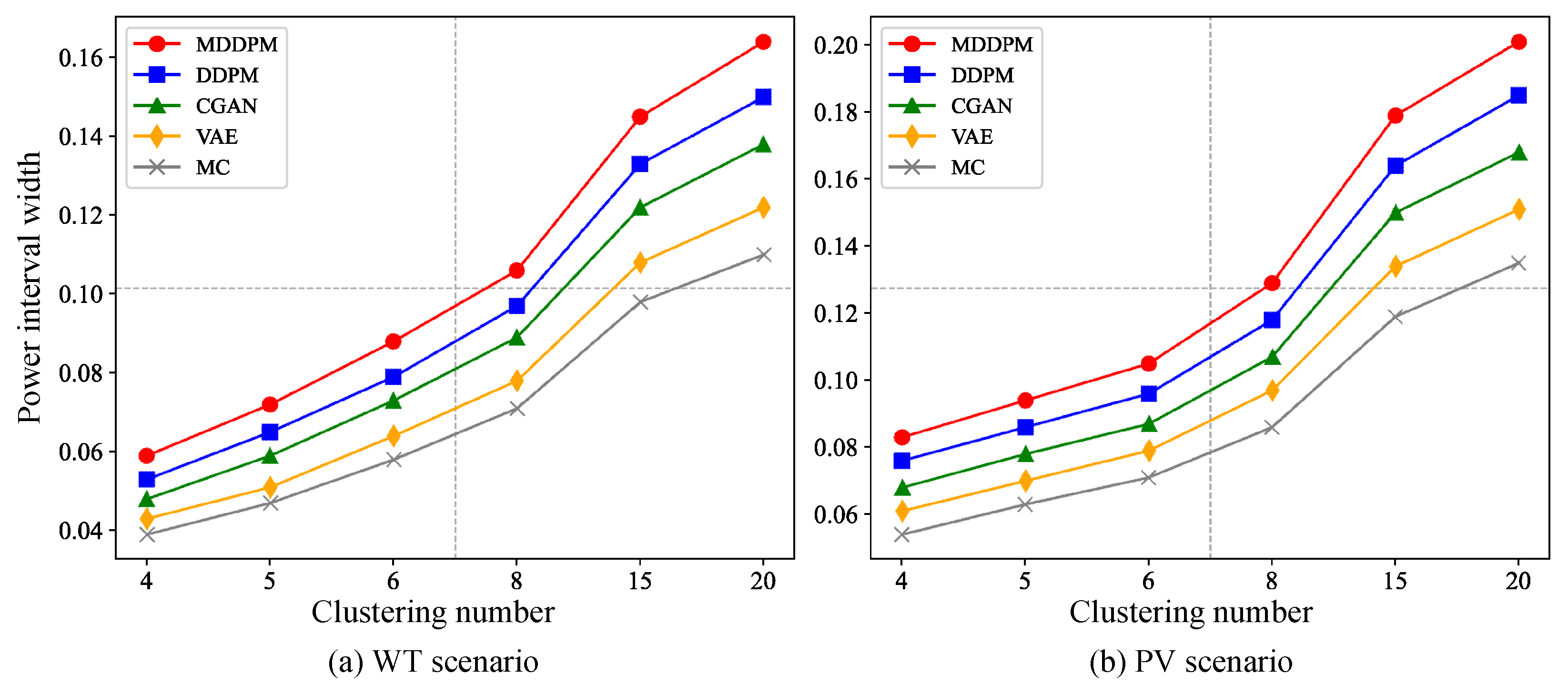
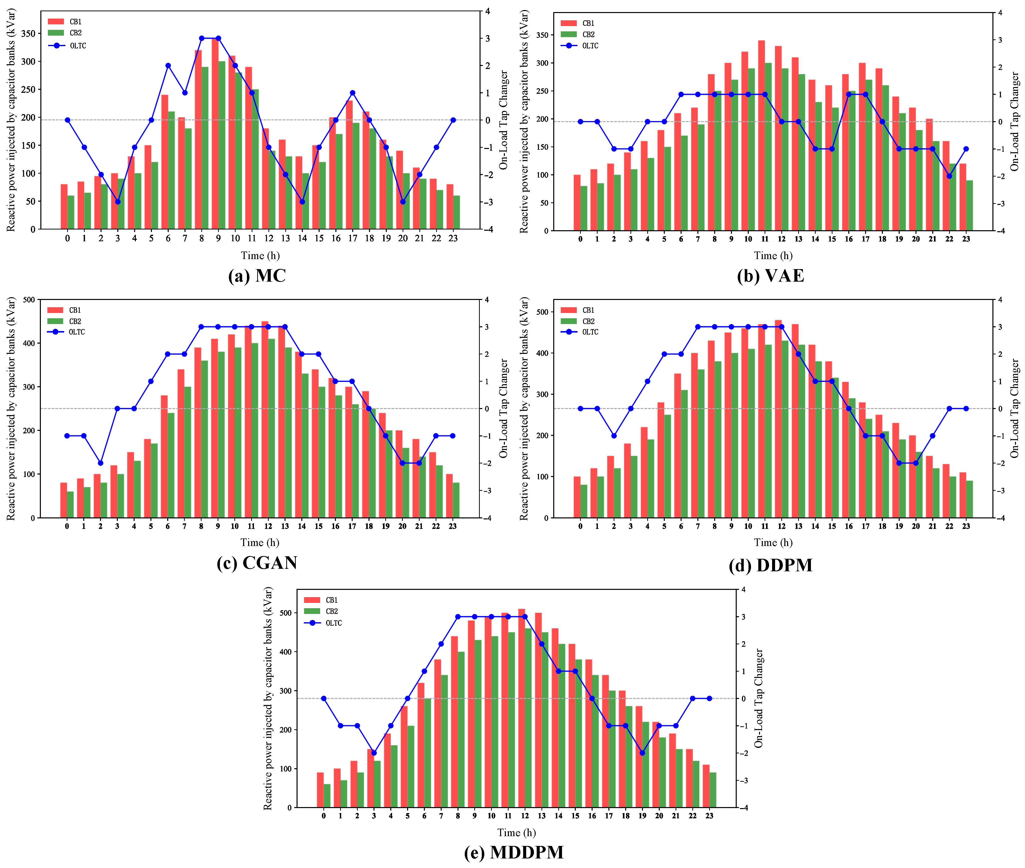
This paper introduces a novel scenario generation framework for wind and photovoltaic power outputs using a Multi-resolution Denoising Diffusion Probabilistic Model (MDDPM). By integrating a multi-scale decomposition strategy and a cascaded conditional denoising diffusion process, this model enhances the accuracy and diversity of generated scenarios, effectively capturing both long-term structural trends (e.g., seasonal variations) and short-term stochastic fluctuations (e.g., daily or weather-related changes). In extensive experiments, the MDDPM outperforms traditional methods, including DDPM, VAE, CGAN, and MC, in terms of scenario accuracy, diversity, and physical consistency.

Despite the promising performance of the proposed MDDPM, there remain areas for future enhancement. The current framework introduces a certain degree of computational overhead due to the multi-resolution structure, which may affect scalability in real-time applications. Additionally, the model’s reliance on historical data quality highlights the importance of robust preprocessing, especially when facing missing or noisy inputs. While our implementation focuses on single-site renewable generation, extending the approach to multi-site or spatially correlated data would further improve its practical applicability. Moreover, balancing accuracy with generalization remains an important consideration to avoid overfitting to historical trends. Incorporating domain-specific physical constraints in future versions could also enhance realism and alignment with real-world operational limits. These aspects represent valuable directions for future work, aiming to further strengthen the model’s flexibility and deployment potential in complex energy systems.

References

1. Chen, Y.; Wang, Y.; Kirschen, D.; Zhang, B. Model-free renewable scenario generation using generative adversarial networks. IEEE Trans. Power Syst. 2018, 33, 3265–3275. [Google Scholar] [CrossRef]
2. Li, J.; Zhou, J.; Chen, B. Review of wind power scenario generation methods for optimal operation of renewable energy systems. Appl. Energy 2020, 280, 115992. [Google Scholar] [CrossRef]
3. Li, Y.; Li, J.; Wang, Y. Privacy-preserving spatiotemporal scenario generation of renewable energies: A federated deep generative learning approach. IEEE Trans. Ind. Inform. 2021, 18, 2310–2320. [Google Scholar] [CrossRef]
4. Gao, S.; Li, Q.; Ding, J.; Liu, W.; Xu, Q.; Li, S. A three-stage optimal energy management strategy for cophase power supply systems with integration of renewable energy. IEEE Trans. Transp. Electrif. 2025, 11, 7599–7614. [Google Scholar] [CrossRef]
5. Chen, J.; Zhao, Y.; Wang, M.; Yang, K.; Ge, Y.; Wang, K.; Lin, H.; Pan, P.; Hu, H.; He, Z.; et al. Multi-timescale reward-based DRL energy management for regenerative braking energy storage system. IEEE Trans. Transp. Electrif. 2025, 11, 7488–7500. [Google Scholar] [CrossRef]
6. Dong, W.; Chen, X.; Yang, Q. Data-driven scenario generation of renewable energy production based on controllable generative adversarial networks with interpretability. Appl. Energy 2022, 308, 118387. [Google Scholar] [CrossRef]
7. Zhang, X.; Glaws, A.; Cortiella, A.; Emami, P.; King, R.N. Deep generative models in energy system applications: Review, challenges, and future directions. Appl. Energy 2025, 380, 125059. [Google Scholar] [CrossRef]
8. da Silva Pereira, E.J.; Pinho, J.T.; Galhardo, M.A.B.; Macêdo, W.N. Methodology of risk analysis by Monte Carlo method applied to power generation with renewable energy. Renew. Energy 2014, 69, 347–355. [Google Scholar] [CrossRef]
9. Yu, J.; Li, Q.; Du, Y.; Wang, R.; Li, R.; Guo, D. Voltage over-limit risk assessment of wind power and photovoltaic access distribution system based on day-night segmentation and Gaussian mixture model. Energy Rep. 2024, 12, 2812–2823. [Google Scholar] [CrossRef]
10. Díaz, G.; Gómez-Aleixandre, J.; Coto, J. Wind power scenario generation through state-space specifications for uncertainty analysis of wind power plants. Appl. Energy 2016, 162, 21–30. [Google Scholar] [CrossRef]
11. Zhou, R.; Chen, S.; Han, Y.; Liu, Q.; Chen, Z.; Hu, W. Probabilistic spatiotemporal scenario generation method for dynamic optimal power flow in distribution networks. Int. J. Electr. Power Energy Syst. 2024, 155, 109667. [Google Scholar] [CrossRef]
12. Guimarães, I.O.; da Silva, A.M.L.; Nascimento, L.C.; Fotuhi-Firuzabad, M. Reliability assessment of distribution grids with DG via quasi-sequential Monte Carlo simulation. Electr. Power Syst. Res. 2024, 229, 110122. [Google Scholar] [CrossRef]
13. Rastgoo, R.; Amjady, N.; Zareipour, H. A deep generative model for selecting representative periods in renewable energy-integrated power systems. Appl. Soft Comput. 2024, 165, 112107. [Google Scholar] [CrossRef]
14. Li, J.; Ye, L.; Zeng, Y.; Wei, H. A scenario-based robust transmission network expansion planning method for consideration of wind power uncertainties. CSEE J. Power Energy Syst. 2016, 2, 11–18. [Google Scholar] [CrossRef]
15. Li, B.; Sedzro, K.; Fang, X.; Hodge, B.-M.; Zhang, J. A clustering-based scenario generation framework for power market simulation with wind integration. J. Renew. Sustain. Energy 2020, 12, 033304. [Google Scholar] [CrossRef]
16. Vagropoulos, S.I.; Kardakos, E.G.; Simoglou, C.K.; Bakirtzis, A.G.; Catalão, J.P.S. ANN-based scenario generation methodology for stochastic variables of electric power systems. Electr. Power Syst. Res. 2016, 134, 9–18. [Google Scholar] [CrossRef]
17. Wang, H.; Xue, W.; Liu, Y.; Peng, J.; Jiang, H. Probabilistic wind power forecasting based on spiking neural network. Energy 2020, 196, 117072. [Google Scholar] [CrossRef]
18. Qi, Y.; Hu, W.; Dong, Y.; Fan, Y.; Dong, L.; Xiao, M. Optimal configuration of concentrating solar power in multienergy power systems with an improved variational autoencoder. Appl. Energy 2020, 274, 115124. [Google Scholar] [CrossRef]
19. Dumas, J.; Cointe, C.; Wehenkel, A.; Sutera, A.; Fettweis, X.; Cornélusse, B. A probabilistic forecast-driven strategy for a risk-aware participation in the capacity firming market. IEEE Trans. Sustain. Energy 2021, 13, 1234–1243. [Google Scholar] [CrossRef]
20. Zhang, Y.; Ai, Q.; Xiao, F.; Hao, R.; Lu, T. Typical wind power scenario generation for multiple wind farms using conditional improved Wasserstein generative adversarial network. Int. J. Electr. Power Energy Syst. 2020, 114, 105388. [Google Scholar] [CrossRef]
21. Li, Z.; Peng, X.; Cui, W.; Xu, Y.; Liu, J.; Yuan, H.; Lai, C.S.; Lai, L.L. A novel scenario generation method of renewable energy using improved VAEGAN with controllable interpretable features. Appl. Energy 2024, 363, 122905. [Google Scholar] [CrossRef]
22. Ho, J.; Jain, A.; Abbeel, P. Denoising diffusion probabilistic models. Adv. Neural Inf. Process. Syst. 2020, 33, 6840–6851. [Google Scholar]
23. Dong, X.; Mao, Z.; Sun, Y.; Xu, X. Short-term wind power scenario generation based on conditional latent diffusion models. IEEE Trans. Sustain. Energy 2023, 15, 1074–1085. [Google Scholar] [CrossRef]
24. Zhao, W.; Shao, Z.; Yang, S.; Lu, X. A novel conditional diffusion model for joint source-load scenario generation considering both diversity and controllability. Appl. Energy 2025, 377, 124555. [Google Scholar] [CrossRef]
25. Liu, H.; Chen, C.; Lv, X.; Wu, X.; Liu, M. Deterministic wind energy forecasting: A review of intelligent predictors and auxiliary methods. Energy Convers. Manag. 2019, 195, 328–345. [Google Scholar] [CrossRef]
26. Li, Y.; Lu, X.; Wang, Y.; Dou, D. Generative time series forecasting with diffusion, denoise, and disentanglement. Adv. Neural Inf. Process. Syst. 2022, 35, 23009–23022. [Google Scholar]
27. Zheng, W.; Chen, Z.; Zheng, K.; Zheng, W.; Chen, Y.; Fan, X. WorkloadDiff: Conditional denoising diffusion probabilistic models for cloud workload prediction. IEEE Trans. Cloud Comput. 2024, 12, 1291–1304. [Google Scholar] [CrossRef]
28. Buła, D.; Grabowski, D.; Lange, A.; Maciążek, M.; Pasko, M. Long- and short-term comparative analysis of RES. Energies 2020, 13, 3610. [Google Scholar] [CrossRef]
29. Hatakeyama, R.; Okuda, K.; Nakashika, T. DDPMVC: Non-parallel any-to-many voice conversion using diffusion encoder. In Proceedings of the 2024 Asia Pacific Signal and Information Processing Association Annual Summit and Conference (APSIPA ASC), Macau, Macao, 3–6 December 2024; APSIPA: Tokyo, Japan, 2024; pp. 1–6. [Google Scholar] [CrossRef]
30. Lu, S.; Guan, F.; Zhang, H.; Lai, H. Speed-Up DDPM for real-time underwater image enhancement. IEEE Trans. Circuits Syst. Video Technol. 2024, 34, 3576–3588. [Google Scholar] [CrossRef]
31. Ho, J.; Saharia, C.; Chan, W.; Fleet, D.J.; Norouzi, M.; Salimans, T. Cascaded diffusion models for high fidelity image generation. J. Mach. Learn. Res. 2022, 23, 1–33. [Google Scholar]
32. Zhou, T.; Ma, Z.; Wen, Q.; Wang, X.; Sun, L.; Jin, R. Fedformer: Frequency enhanced decomposed transformer for long-term series forecasting. In Proceedings of the International Conference on Machine Learning, Baltimore, MD, USA, 17–23 July 2022; PMLR: Baltimore, MD, USA, 2022; pp. 27268–27286. [Google Scholar]
Figure 1. The proposed MDDPM framework.
Energies 18 03781 g001
Figure 2. The conditioning network and denoising network.
Energies 18 03781 g002
Figure 3. DDPM (without seasonal-trend decomposition blocks).
Energies 18 03781 g003
Figure 4. Training evolution of training set.
Energies 18 03781 g004
Figure 5. Comparison of power interval widths generated by different methods for scenarios at different clustering levels.
Energies 18 03781 g005
Figure 6. Comparison of global coverage of scenario generation by different methods at different clustering levels.
Energies 18 03781 g006
Figure 7. Impact of different scenario generation methods on power grid dispatch optimization for IEEE 33-node system.
Energies 18 03781 g007