Well Production Forecasting in Volve Field Using Kolmogorov–Arnold Networks

Abstract

Accurate oil production forecasting is essential for optimizing field development and supporting efficient decision-making. However, traditional methods often struggle to capture the complex dynamics of reservoirs, and existing machine learning models rely on large parameter sets, resulting in high computational costs and limited scalability. To address these limitations, we propose the Kolmogorov–Arnold Network (KAN) for oil production forecasting, which replaces traditional weights with spline-based learnable activation functions to enhance nonlinear modeling capabilities without large-scale parameter expansion. This design reduces training costs and enables adaptive scaling. The KAN model was applied to forecast oil production from wells 15/9-F-11 and 15/9-F-14 in the Volve field, Norway. The experimental results demonstrate that, compared to the best-performing baseline model, the KAN reduces the Mean Absolute Error (MAE) and Root Mean Squared Error (RMSE) by 78.5% and 89.5% for well 15/9-F-11 and by 80.1% and 91.8% for well 15/9-F-14, respectively. These findings suggest that the KAN is a robust and efficient multivariate forecasting method capable of capturing complex dependencies in oil production data, with strong potential for practical applications in reservoir management and production optimization.

1. Introduction

The oil industry, as a critical pillar of the global energy system, not only plays an indispensable role in economic development but also faces significant challenges during energy transition [1]. In recent years, with the gradual depletion of oil resources and increasing extraction difficulties, the need to enhance development efficiency and resource utilization within the industry has grown significantly [2]. Market uncertainties, price fluctuations, and the pressures of climate change have further driven oil companies to seek more precise and efficient solutions. Against this backdrop, production forecasting, as a core task in oilfield management and development planning, has garnered widespread attention [3].

Traditional methods for oil forecasting include Decline Curve Analysis (DCA) and numerical reservoir simulation (NRS). DCA is an empirical method based on historical production data from oilfields, mainly used to predict future production and remaining recoverable reserves by analyzing the declining trend of oilfield output over time [4,5]. The core principle is that oilfield production will undergo a stable decline, which can be described using different types of decline curves [6]. DCA is comparatively simple to calculate and requires relatively little data, which makes it very practical in the early stage of oilfield development or when data are limited [7]. However, its assumptions are oversimplified and fail to fully consider the complexity of reservoirs, such as petrophysical properties and formation pressure, so it is difficult to be applied to unconventional reservoirs [8]. On the other hand, NRS is a technique that uses numerical methods to dynamically simulate reservoirs [9]. It creates a mathematical model of a reservoir by integrating geological, physical, and fluid parameters and employs numerical methods to solve processes like fluid flow, pressure variations, and heat transfer within the reservoir [10]. It can account for the reservoir’s complex geological structure, heterogeneity, nonlinear flow, and different types of extraction methods, simulating the movement of oil and gas within the reservoir and predicting the long-term production behavior of the oilfield. But, for realistic applications, it requires large computational resources, high data demands, and complex model construction.

Traditional production forecasting methods rely on physical models and empirical rules, which work well when historical data is abundant, but their accuracy is limited when data support is lacking [11]. To address this issue, the rapid development of computer technology has brought transformative tools and methods to oil production forecasting. Machine learning is gradually replacing traditional methods, becoming the mainstream solution for addressing production forecasting issues [12,13]. Simple models such as support vector regression (SVR) and Multilayer Perceptrons (MLPs) were previously used to predict oil production and achieved some success. However, due to its monolithic structure, a single neural network model struggles with low predictive stability and poor generalization when dealing with strongly nonlinear, multiscale, and complex time-series data like oil and gas production [14]. With the development of neural networks, the hybrid neural network model gives full play to their respective strengths by combining various network structures such as Transformer, Long Short-Term Memory (LSTM) networks and attention mechanisms to achieve the efficient extraction and dynamic weighting processing of multi-level and multi-scale features, which effectively improves prediction accuracy. Compared to traditional regression methods, Temporal Fusion Transformer (TFT) combines the advantages of attention mechanisms and recurrent neural networks and is specifically designed for time-series forecasting [15]. It is particularly suitable for handling time-series data in the oil industry as it can focus on both long-term and short-term dependencies between oil production and other features, such as pressure, temperature, and permeability, thereby providing more accurate predictions [16,17]. TFT uses self-attention mechanisms to dynamically focus on key information within the sequence while enhancing data modeling through LSTM networks. On the other hand, Bidirectional Long Short-Term Memory with Attention (Bi-LSTM Attention) combines the strengths of bidirectional LSTM and attention mechanisms, enabling the model to learn information from both the forward and backward directions of the sequence, focusing on the changes in oil production over time, thus enhancing the model’s expressive power [18,19]. Bi-LSTM Attention is also suitable for capturing complex temporal dependencies in oil production data [20].

Although hybrid models improve prediction accuracy by integrating multiseed models, they inevitably introduce a large number of learnable parameters, which poses a number of problems: training time and computational overhead increase significantly. In addition, the black-box nature of the hybrid model further reduces interpretability, which is particularly unfavorable for oil and gas production scenarios that are highly dependent on engineering experience. To better predict oil production, we propose to use the KAN model for well-production forecasting. The KAN is a novel neural network architecture that is fundamentally different from traditional feedforward networks in its handling of nonlinearities and function representations [21]. Unlike MLPs, which rely on fixed activation functions applied after linear transformation, the KAN is inspired by the Kolmogorov–Arnold representation theorem and uses trainable univariate functions to directly parameterize nonlinear mappings [22,23]. This design allows the KAN to intrinsically model highly nonlinear relationships without the need to build deep network architectures as in hybrid models such as TFT, resulting in greater expressiveness with fewer parameters. The core strength of the KAN lies in its use of the B-spline function, which provides an adaptive approximation of fine-grained functions [24]. By dynamically refining the spline grid, the KAN can model complex patterns with high efficiency and accuracy, ensuring smooth and flexible function interpolation. In addition, unlike traditional neural networks that need to be retrained when expanding the model capacity, the KAN supports progressive refinement, which allows coarser models to be refined into finer ones without the need to retrain from scratch [25,26]. These innovations allow the KAN model to leverage powerful non-linear modeling capabilities, providing a new solution for oil production forecasting.

In this study, we used the KAN to predict oil production from wells 15/9-F-11 and 15/9-F-14 in the Norwegian Volve field and evaluate the predictive performance of these models in comparison with TFT and Bi-LSTM Attention.

The rest of this paper is organized as follows: The reservoir and well description provides an overview of the Volve oilfield, including its geographical location. Section 3 provides a detailed explanation of the proposed model, including SVR, TFT, Bi-LSTM Attention, and the KAN. Section 4 covers the dataset preparation steps, the evaluation metrics used, and the parameter optimization. Section 5 presents and discusses the findings from the experiments. Finally, Section 6 summarizes the contributions of this paper and discusses future research directions.

2. Reservoir and Well Description

Located about 200 km offshore in the Norwegian sector of the North Sea, the Volve field is a major oil and gas reservoir operated by Equinor, with Petoro and TotalEnergies as major partners. Discovered in 1974 and developed in the early 2000s, it lies at water depths of 330 to 380 m within the Vøring Basin, near fields such as Åsgard and Ormen Lange [27]. The field features Late Jurassic and Cretaceous reservoirs with recoverable reserves of several hundred million barrels of oil equivalent. Developed with 56 wells, including production, injection, and observation wells, Volve was under construction from 2008 to 2016. Its high-resolution three-dimensional (3D) reservoir model, comprising 22 million grid cells, and its extensive dataset—including seismic surveys, well logs, and production metrics—make it a valuable resource for research in subsurface analysis, reservoir management, and petroleum engineering [12].

3. Methodology

3.1. Support Vector Regression (SVR)

SVR is a specialized extension of the Support Vector Machine (SVM) algorithm, specifically designed to handle regression tasks. As an advanced supervised machine learning method, SVR utilizes input data to predict continuous output values [28]. The goal of SVR is to build a function that approximates the relationship between the input vector $x=\{x_1,x_2,\dots ,x_k\}$ and the corresponding output vector $y=\{y_1,y_2,\dots ,y_k\}$, in which $x_j\in \mathbb{R}$, where k represents the total number of data points.

The regression function is generally expressed as follows:

$$f\left(x\right)=w·\Psi \left(x\right)+b$$

(1)

where $\Psi \left(x\right)$ is the mapping of the input vector x into a higher-dimensional feature space, which allows the original nonlinear regression problem to be transformed into a linear one. In this formulation, w is the weight vector, and b is the bias term. To determine these parameters, the following regularized risk function is minimized:

$$E\left(C\right)={\displaystyle \frac{C}{k}}\sum _{j=1}^{k}L(f\left(x_j\right)-y_j)+{\displaystyle \frac{1}{2}}{\left|\right|w\left|\right|}^2.$$

(2)

In Equation (2), the first term measures the empirical error, while the second term regularizes the function’s complexity. The penalty constant C controls the balance between fitting the model to the data and minimizing the model’s complexity.

To address empirical errors, Vapnik introduced the $ϵ$-insensitive loss function, defined as follows:

$$L(f\left(x\right)-y)=\left\{\begin{array}{cc}0,\hfill & \mathrm{if}\left|f\right(x)-y|\le ϵ\hfill \\ \left|f\right(x)-y|-ϵ,\hfill & \mathrm{otherwise}.\hfill \end{array}\right.$$

(3)

Here, $ϵ$ defines a tolerance margin within which predictions are considered acceptable. Incorporating this loss function, the optimization problem can be reformulated as follows:

$$\underset{C}{min}\left\{\sum _{j=1}^k({\xi }_j^{+}+{\xi }_j^{-})+{\displaystyle \frac{1}{2}}{\left|\right|w\left|\right|}^2\right\}$$

(4)

subject to the following constraints:

$$\left\{\begin{array}{c}{y}_j-(w·\Psi \left(x_j\right)+b)\le ϵ+{\xi }_j^{+}\hfill \\ (w·\Psi \left(x_j\right)+b)-y_j\le ϵ+{\xi }_j^{-}\hfill \\ {\xi }_j^{+},{\xi }_j^{-}\ge 0,\mathrm{for}j=1,2,\dots ,k.\hfill \end{array}\right.$$

(5)

Here, ${\xi }_j^{+}$ and ${\xi }_j^{-}$ are non-negative slack variables that capture any deviations outside the margin defined by $ϵ$. This constrained optimization problem can be efficiently solved using the Lagrangian dual formulation, leading to the dual solution expressed as follows:

$$f\left(x\right)=\sum _{j=1}^k({\alpha }_j^{*}-{\alpha }_j)K(x_j,x_m)+b$$

(6)

where ${\alpha }_j$ and ${\alpha }_j^{*}$ are the Lagrange multipliers satisfying the conditions $0\le {\alpha }_j^{*}\le C$. The kernel function $K(x_j,x_m)$ is responsible for mapping the data points into a higher-dimensional space implicitly.

SVR can employ various kernel functions, including polynomial, Gaussian, and radial basis function (RBF) kernels. A commonly used RBF kernel is defined as follows:

$$K(x_j,x_m)=exp(-\gamma ||x_j-x_m{\left|\right|}^2)$$

(7)

where $\gamma$ is the kernel parameter. The performance of SVR is sensitive to the choice of hyperparameters $\gamma$, C, and $ϵ$. Metaheuristic algorithms are often employed to optimize these hyperparameters, providing a systematic approach to enhancing SVR’s performance. These algorithms offer a more efficient alternative to traditional trial-and-error techniques [28], resulting in improved predictive accuracy by systematically searching the parameter space [29].

3.2. Temporal Fusion Transformer

TFT is an advanced deep learning architecture built upon attention mechanisms, specifically designed for multi-horizon forecasting. It achieves a balance between high predictive accuracy and interpretability [15]. By integrating sequence-to-sequence modeling with interpretable multi-head attention, TFT effectively captures both short-term dynamics and long-range dependencies, making it well-suited for complex time-series forecasting tasks [17]. Figure 1 shows the high-level architecture of TFT.

TFT employs variable selection networks to filter input variables, reducing redundancy and focusing on the most predictive features. At each time step t, the transformed input variables are denoted as ${\Xi }_t$, and the variable selection weights are computed using a Gated Residual Network (GRN) followed by a softmax function:

$$v_t^{\chi }=\mathrm{Softmax}\left({\mathrm{GRN}}_v({\Xi }_t,c_s)\right)$$

(8)

where $c_s$ is a context vector generated by the static covariate encoder.

The static covariate encoders utilize GRNs to generate context vectors $c_s,c_e,c_c,c_h$, which influence temporal modeling, variable selection, and information fusion. For example, $c_s$ is primarily used for variable selection, while $c_e$ is employed for static enrichment of temporal features.

For temporal modeling, TFT integrates local processing and self-attention mechanisms. Short-term dependencies are captured by an LSTM-based encoder–decoder, while long-term dependencies are learned via the Interpretable Multi-Head Attention Layer:

$$\mathrm{Attention}(Q,K,V)=\mathrm{Softmax}\left({\displaystyle \frac{Q{K}^T}{\sqrt{d_{\mathrm{attn}}}}}\right)V.$$

(9)

To enhance interpretability, TFT applies a shared value mechanism in multi-head attention and computes the final attention weights using additive aggregation:

$$\tilde{H}={\displaystyle \frac{1}{m_H}}\sum _{h=1}^{m_H}\mathrm{Attention}(Q{W}_Q^{\left(h\right)},K{W}_K^{\left(h\right)},V{W}_V).$$

(10)

In the Temporal Fusion Decoder, TFT introduces the static enrichment layer and the position-wise feedforward layer to further extract and fuse temporal information. The static enrichment layer applies GRNs to process temporal features:

$$\theta (t,n)={\mathrm{GRN}}_{\theta }(\tilde{\varphi }(t,n),c_e)$$

(11)

while the position-wise feedforward layer performs additional nonlinear transformations with optional residual skip connections:

$$\tilde{\psi }(t,n)=\mathrm{LayerNorm}(\tilde{\varphi }(t,n)+\mathrm{GLU}\left(\psi (t,n)\right)).$$

(12)

For uncertainty estimation, TFT employs Quantile Regression to predict confidence intervals. Given a target variable y and its predicted value $\widehat{y}$, TFT optimizes the quantile loss function:

$$L(y,\widehat{y},q)=q{(y-\widehat{y})}^{+}+(1-q){(\widehat{y}-y)}^{+}$$

(13)

which enables the model to generate forecasts for different quantile levels.

In summary, TFT effectively captures nonlinear relationships and temporal dependencies in complex multivariate forecasting tasks through its multi-layer attention structure and variable selection mechanism, offering a powerful and interpretable tool for multi-horizon time series forecasting.

3.3. Bidirectional Long Short-Term Memory with Attention

Bi-LSTM Attention is a neural network model that combines Bidirectional Long Short-Term Memory (Bi-LSTM) and attention mechanisms, primarily used for tasks like relation classification [19]. Its primary objective is to capture the most important semantic information from input sequences, improving classification accuracy while reducing reliance on external feature engineering and linguistic resources [18]. The core idea of Bi-LSTM is to use two LSTM networks, with one processing the input sequence forward and the other backward, allowing the model to capture both past and future contextual information simultaneously. This bidirectional structure enables comprehensive modeling of sequential data. For each time step in the input sequence, Bi-LSTM generates a forward hidden state $\overrightarrow{h_t}$ and a backward hidden state $\overleftarrow{h_t}$, which are concatenated to form the output representation of that time step:

$$h_t=\overrightarrow{h_t}\oplus \overleftarrow{h_t}$$

(14)

where ⊕ denotes vector concatenation.

To further enhance the model’s ability to focus on the most critical parts of the sequence, an attention mechanism is incorporated. The attention mechanism assigns a weight to each time step’s output, allowing the model to automatically select the most important parts of the sequence for the task, thereby generating a global sentence representation. The attention weights are computed through a nonlinear transformation of the input features, as shown below:

$$\begin{array}{cc}\hfill M& =tanh\left(H\right)\hfill \end{array}$$

(15)

$$\begin{array}{cc}\hfill \alpha & =\mathrm{softmax}\left(w^{T}M\right)\hfill \end{array}$$

(16)

$$\begin{array}{cc}\hfill r& =H{\alpha }^T.\hfill \end{array}$$

(17)

Here, H is the matrix consisting of all hidden states produced by Bi-LSTM for all time steps, M is an intermediate representation obtained through a nonlinear transformation, $\alpha$ represents the normalized attention weights, and r is the global sentence representation obtained through a weighted sum.

The final sentence representation r is passed to a classifier, which uses the softmax function to predict the relationship type. The formula for the classifier is as follows:

$$\widehat{y}=\mathrm{softmax}(Wr+b)$$

(18)

where W and b are learnable parameters.

The simple architecture of Bi-LSTM Attention is shown in Figure 2. The bidirectional LSTM can capture both long-term and short-term dependencies within input sequences, while the attention mechanism enhances the model’s ability to focus on critical information, improving its interpretability [30]. Additionally, this method does not rely on external feature engineering and can achieve efficient modeling solely through word embeddings and sequential data.

3.4. Kolmogorov–Arnold Networks

MLPs extend the classical perceptron framework, rooted in the universal approximation theorem. This theorem guarantees that a feedforward neural network with a single hidden layer and finite width can approximate any continuous function over compact subsets of ${\mathbb{R}}^n$. In contrast, the KAN is grounded in the Kolmogorov–Arnold representation theorem [23], which establishes that any multivariate continuous function on a bounded domain can be expressed as a finite composition of univariate functions and additive operations. Formally, for a smooth function $f:{[0,1]}^n\to \mathbb{R}$,

$$f\left(\mathbf{x}\right)=\sum _{q=1}^{2n+1}\sum _{p=1}^n{\varphi }_{q,p}\left(x_p\right)$$

(19)

where ${\varphi }_{q,p}:[0,1]\to \mathbb{R}$ are learnable univariate mappings. This decomposition underscores the foundational role of addition in multivariate function representation, with all higher-order interactions subsumed into univariate components. A KAN layer, defined as a matrix of 1D functions, maps $n_{\mathrm{in}}$-dimensional inputs to $n_{\mathrm{out}}$-dimensional outputs:

$$\mathbf{\Phi }=\left\{{\varphi }_{q,p}\right\},p=1,2,\dots ,n_{\mathrm{in}},q=1,2,\dots ,n_{\mathrm{out}}.$$

(20)

The inner functions in the theorem correspond to a KAN layer transforming $n_{\mathrm{in}}=n$ to $n_{\mathrm{out}}=2n+1$, while the outer layer reduces dimensionality to a scalar output.

A KAN’s architecture is specified by an integer sequence:

$$[n_0,n_1,\dots ,n_L]$$

(21)

where $n_i$ denotes neuron count in the i-th layer. Let $(i,j)$ index the j-th neuron in layer i, with activation $x_{i,j}$. Between layers i and $i+1$, $n_i\times n_{i+1}$ activation functions link neurons pairwise. The function connecting $(i,j)$ to $(i+1,k)$ is denoted ${\varphi }_{i,j,k}$. The activation of neuron $(i+1,k)$ aggregates post-activations from all predecessors:

$$x_{i+1,k}=\sum _{j=1}^{n_i}{\varphi }_{i,j,k}\left(x_{i,j}\right)$$

(22)

which in matrix form becomes the following:

$${\mathbf{X}}_{i+1}={\Phi }_i·{\mathbf{X}}_i$$

(23)

where ${\Phi }_i$ is the function matrix corresponding to the i-th KAN layer. The full network output is a layered composition:

$$\mathrm{KAN}\left(\mathbf{x}\right)={\Phi }_{L-1}·{\Phi }_{L-2}·\dots ·{\Phi }_0·{\mathbf{x}}_0.$$

(24)

By contrast, MLPs interleave affine transformations $\mathit{W}$ and fixed nonlinearities $\sigma$:

$$\mathrm{MLP}\left(\mathbf{x}\right)=\left({\mathit{W}}_{L-1}\circ \sigma \circ {\mathit{W}}_{L-2}\circ \dots \circ \sigma \circ {\mathit{W}}_0\right)\mathbf{x}.$$

(25)

While MLPs decouple linear and nonlinear operations, KANs unify them via function matrices $\mathbf{\Phi }$, as depicted in Figure 3.

To enhance training efficiency, KANs integrate residual structures by decomposing activation functions into a basis term $b\left(x\right)$ and a spline component:

$$\varphi \left(x\right)=w\left(b\left(x\right)+\mathrm{spline}\left(x\right)\right)$$

(26)

where $b\left(x\right)$ is typically a sigmoidal function:

$$b\left(x\right)=\mathrm{sigm}\left(x\right)={\displaystyle \frac{x}{1+e^{-x}}}.$$

(27)

The spline term employs B-splines with trainable coefficients:

$$\mathrm{spline}\left(x\right)=\sum _i{c}_i{B}_i\left(x\right).$$

(28)

During training, spline grids dynamically adapt to input distributions, resolving boundary mismatch issues.

KANs achieve high precision through adaptive grid refinement. For a 1D function f on $[a,b]$, a coarse grid $G_1$ with knots $\{t_0=a,\dots ,t_{G_1}=b\}$ is extended to the following:

$$\{t_{-k},\dots ,t_1,t_0,t_1,\dots ,t_{G_1+k}\}$$

(29)

yielding $G_1+k$ B-spline bases. The coarse approximation is as follows:

$$f_{\mathrm{coarse}}\left(x\right)=\sum _{i=0}^{G_1+k-1}{\widehat{c}}_i{B}_i\left(x\right).$$

(30)

Refining to $G_2$ intervals produces the following:

$$f_{\mathrm{fine}}\left(x\right)=\sum _{i=0}^{G_2+k-1}{c}_i{B}_i\left(x\right)$$

(31)

where parameters $c_i$ are initialized via least-squares minimization:

$$c_i=\arg \min \left(\sum _{i=0}^{G_2+k-1}{\left[f_{\mathrm{fine}}\left(x\right)-f_{\mathrm{coarse}}\left(x\right)\right]}^2\right).$$

(32)

This strategy enables incremental accuracy gains without retraining, circumventing MLPs’ reliance on brute-force scaling. By decoupling model complexity from computational overhead, KANs achieve superior parameter efficiency, which is particularly advantageous in large-scale applications.

4. Experiments

In this study, we used TFT, Bi-LSTM Attention, and KAN models to predict oil production rates from wells 15/9-F-11 and 15/9-F-14 in the Volve field offshore the North Sea. Each well consists of the data as shown in

Table 1. Data provided for each well in the Volve field.

Abbreviation from Database	Description
BORE_OIL_VOL	Oil Volume from Well
Time	Date of Record
ON_STREAM_HRS	On Stream Hours
AVG_DOWNHOLE_PRESSURE	Average Downhole Pressure
AVG_DOWNHOLE_TEMPERATURE	Average Downhole Temperature
AVG_DP_TUBING	Average Differential Pressure of Tubing
AVG_ANNULUS_PRESS	Average Annular Pressure
AVG_CHOKE_SIZE_P	Average Choke Size Percentage
AVG_WHP_P	Average Wellhead Pressure
AVG_WHT_P	Average Wellhead Temperature
DP_CHOKE_SIZE	Differential Pressure across the Choke
BORE_GAS_VOL	Gas Volume from Well
BORE_WAT_VOL	Water Volume from Well

.

4.1. Data Preprocessing

Transforming raw data into a suitable format for model input is an essential step in data preprocessing for neural network models. The procedure involves dealing with missing values, normalizing features, and encoding categorical variables to boost data quality and maintain stability and performance during model training.

Daily measurements from the Volve field were used in this research. Because it is too costly to perform calculations using data from all wells, two wells, well 15/9-F-11 and well 15/9-F-14, were selected for their representative and high-quality production data to ensure a high-quality study with limited resources. Data for well 15/9-F-11 range from 2013 to 2016, while data for well 15/9-F-14 cover the period from 2008 to 2016. However, the raw data contain missing values, which were filled in using forward linear interpolation, a method that estimates missing data by averaging the known data points.

4.2. Data Exploration

Data exploration aims to uncover the structure, patterns, trends, and potential issues within the data, clarifying its characteristics and guiding subsequent modeling and analysis. Before modeling, relationships between different variables are explored through data visualization, with heatmaps of Pearson correlation coefficients commonly used [31]. These heatmaps visually represent the linear correlation between variables, with values ranging from −1 to +1, indicating the strength of negative to positive correlations. They help identify potential correlations and multicollinearity issues.

The dataset comprises temporal monitoring parameters for individual wells, including date, average downhole pressure, average downhole temperature, average drill pipe pressure, average annular pressure, average tubing diameter, average wellhead pressure, average wellhead temperature, and liquid production volumes (oil/gas/water). In this study, BORE_OIL_VOL is designated as the target variable. Feature screening is conducted by calculating Pearson correlation coefficients between this target and other parameters. Parameters with excessive correlation are systematically excluded. For Well 15/9-F-11, due to the small sample size of the dataset, we selected the top five features with the strongest correlations with the target variable to avoid overfitting. For Well 15/9-F-14, which has a larger sample size, we selected the top six features with the strongest correlation to the target variable.

Figure 4 displays the correlation heatmap for Well 15/9-F-11. After screening, the final selected features for machine learning modeling included Time, ON_STREAM_HRS, AVG_DP_TUBING, AVG_CHOKE_SIZE_P, and AVG_WHT_P.

The correlation distribution for Well 15/9-F-14 is visualized in Figure 5. Through identical screening protocols, the feature space is constructed using Time, ON_STREAM_HRS, AVG_DOWNHOLE_PRESSURE, AVG_DP_TUBING, AVG_CHOKE_SIZE_P, and AVG_WHT_P.

This differential threshold strategy effectively balances feature informativeness against model complexity, ensuring selected parameters capture significant relationships while maintaining variable independence.

4.3. Data Partitioning

In this study, the dataset was divided into two parts: one for training and one for testing. Specifically, 80% of the data was used to train the model, while the remaining 20% was used for testing. This strategy improves the model’s ability to generalize and increases its overall predictive accuracy.

4.4. Evaluation Metrics

Common evaluation metrics in time series forecasting include the coefficient of determination (R²), MAE, mean squared error (MSE), and RMSE. In this study, for oil production forecasting we used MAE and RMSE to evaluate the model performance.

MAE measures the average absolute difference between the true values ($y_i$) and the predicted values (${\widehat{y}}_i$), which is defined as follows:

$$\mathrm{MAE}={\displaystyle \frac{1}{n}}\sum _{i=1}^n|y_i-{\widehat{y}}_i|$$

(33)

where n denotes the number of data points. MAE provides a straightforward measure of the average magnitude of the prediction errors. RMSE, the square root of the mean squared error, quantifies the magnitude of prediction errors in the same unit as the target variable, calculated as follows:

$$\mathrm{RMSE}=\sqrt{{\displaystyle \frac{1}{n}}\sum _{i=1}^n{(y_i-{\widehat{y}}_i)}^2}.$$

(34)

By combining these two metrics, MAE offers an intuitive interpretation of average prediction error, while RMSE captures the overall error magnitude, placing greater emphasis on larger deviations. This combination provides a balanced evaluation of the model’s predictive accuracy and robustness.

4.5. Parameter Optimization

In order to improve the performance of the proposed model, the hyperparameters were tuned using a grid search strategy. Grid search is an exhaustive search technique that evaluates all possible combinations of the specified hyperparameters to determine the best configuration. In this study, key hyperparameters, including the number of cells per layer, learning rate, batch size, and dropout rate, were optimized.

Table 2. Optimal hyperparameters for the best SVR model.

Parameter	Value
Kernel	linear
C	0.1
Epsilon	0.1

shows the hyperparameters of the best SVR model. Through the combination of these parameters, the model achieves the best regression performance while balancing bias and variance.

Table 3. Network architecture of the best TFT model.

Layer Type	Output Shape
Input	(30, 7)
LSTM	(30, 128)
LayerNormalization	(30, 128)
Dropout	(30, 128)
MultiHeadAttention	(30, 128)
Concatenate	(30, 256)
LSTM	(128)
LayerNormalization	(128)
Dropout	(128)
Dense	(1)

presents the network architecture of the best TFT model, which leverages an LSTM-based sequence modeling approach combined with multi-head attention, layer normalization, and dropout to capture long-term dependencies in time series data.

Table 4. Optimal hyperparameters for the best TFT model.

Parameter	Value
Random seed	12,345
Lookback	30
N_ahead	1
Number of LSTM units	128
Number of LSTM layers	2
Dropout rate	0.2
Number of attention heads	4
Key dimension in multi-head attention	7
Batch size	64
Optimizer	RMSprop
Learning rate	$1\times {10}^{-4}$
Loss function	MSE
Early stopping patience	20
Validation split	10%
Epochs	100

summarizes the optimal hyperparameters for this model, including LSTM units, attention heads, batch size, learning rate, and early stopping criteria.

Table 5. Network architecture of the best Bi-LSTM-Attention model.

Layer Type	Output Shape
Input	(30, 7)
Bidirectional LSTM	(30, 100)
Dropout	(30, 100)
MultiHeadAttention	(30, 100)
Dropout	(30, 100)
Bidirectional LSTM	(100)
Dense	(100)
Multiply	(100)
Dense	(1)

outlines the architecture of the best Bi-LSTM-Attention model, which enhances temporal feature extraction by using bidirectional LSTM layers, attention mechanisms, and a multiplication operation to refine feature representations.

Table 6. Optimal hyperparameters for the best Bi-LSTM-Attention model.

Parameter	Value
Random seed	12,345
Lookback	30
N_ahead	1
Number of LSTM units	50
Number of Bidirectional LSTM layers	2
Dropout rate	0.2
Number of attention heads	4
Key dimension in multi-head attention	25
Batch size	96
Optimizer	Adam
Learning rate	$1\times {10}^{-4}$
Loss function	MSE
Early stopping patience	20
Validation split	10%
Epochs	100

details its optimized hyperparameters, covering the number of LSTM units, dropout rates, attention heads, optimizer choice, and training parameters.

Table 7. Network architecture of the best KAN model.

Layer Type	Output Shape
Input Layer	(2)
Kolmogorov–Arnold Layer 1	(5)
Activation Function	(5)
Kolmogorov–Arnold Layer 2	(1)
Activation Function	(1)
Output Layer	(1)

describes the architecture of the best KAN model, which is built upon the Kolmogorov–Arnold representation theorem, offering an alternative to traditional neural networks by replacing matrix-based transformations with adaptive spline-based function approximators.

Table 8. Optimal hyperparameters for the best KAN model.

Parameter	Value
Random seed	1234
KAN layer widths	[2, 5, 1]
Grid	3
Spline order	3
Activation function	Adaptive Spline
Optimizer	LBFGS
Loss function	MSE
Epochs	100

lists the optimal hyperparameters for the KAN, including the grid size, spline order, activation function, optimizer, and training settings.

Notably, the KAN achieves competitive predictive accuracy with significantly fewer parameters compared to LSTM-based models, owing to its ability to refine function approximations by adjusting the granularity of spline grids rather than increasing network depth or width. This property allows the KAN to scale more efficiently, requiring lower computational costs while maintaining high expressivity and generalization.

5. Results and Discussion

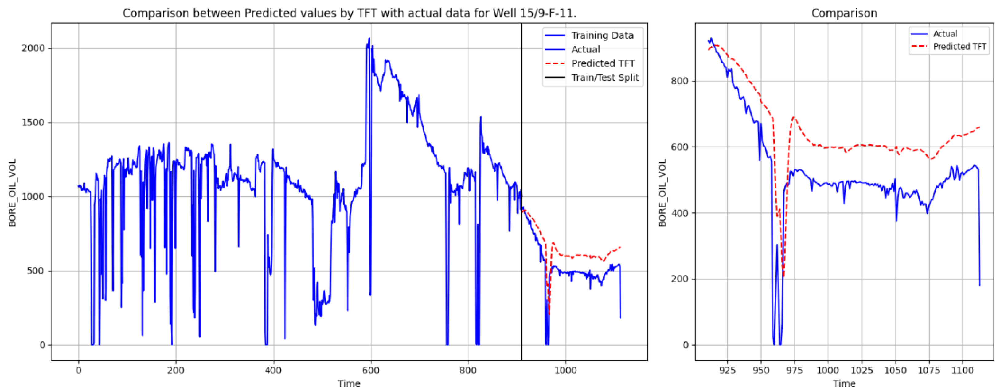
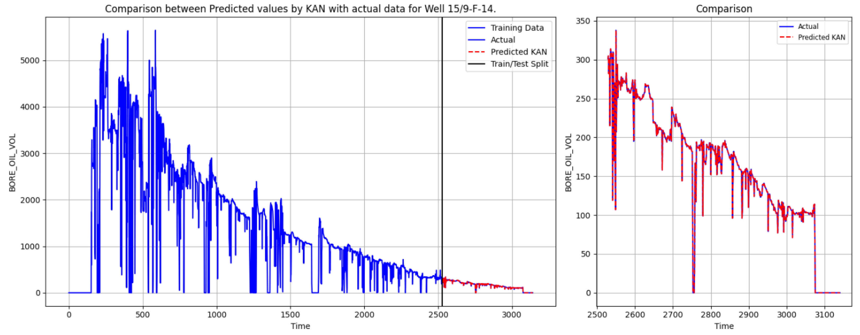
To evaluate the predictive capabilities of different deep learning models for oil production forecasting, we conducted a comparative analysis using SVR, TFT, Bi-LSTM-Attention, and the KAN. The objective was to assess their ability to capture complex temporal dependencies and produce accurate forecasts. The results for Well 15/9-F-11 are depicted in Figure 6, Figure 7, Figure 8 and Figure 9. These figures demonstrate the performance of different models in predicting oil production, evaluating the accuracy of their predictions by comparing them with actual data. Each chart consists of two parts: the left side shows the overall performance of the training data and model predictions, while the right side zooms in on the details of the test set. The blue curve represents the actual data, the red dashed line indicates the predicted values, and the black vertical line marks the boundary between the training and test sets.

Figure 6 shows that the SVR model’s prediction of the production rate for Well 15/9-F-11 follows the overall trend of the actual data, but there is some deviation between the predicted and actual values in the local details. Figure 7 presents the comparison between TFT predictions and actual oil production data. From an overall perspective, TFT effectively captures the declining trend of oil production. However, in the later phase of the test period, its predictions tend to overestimate actual values. 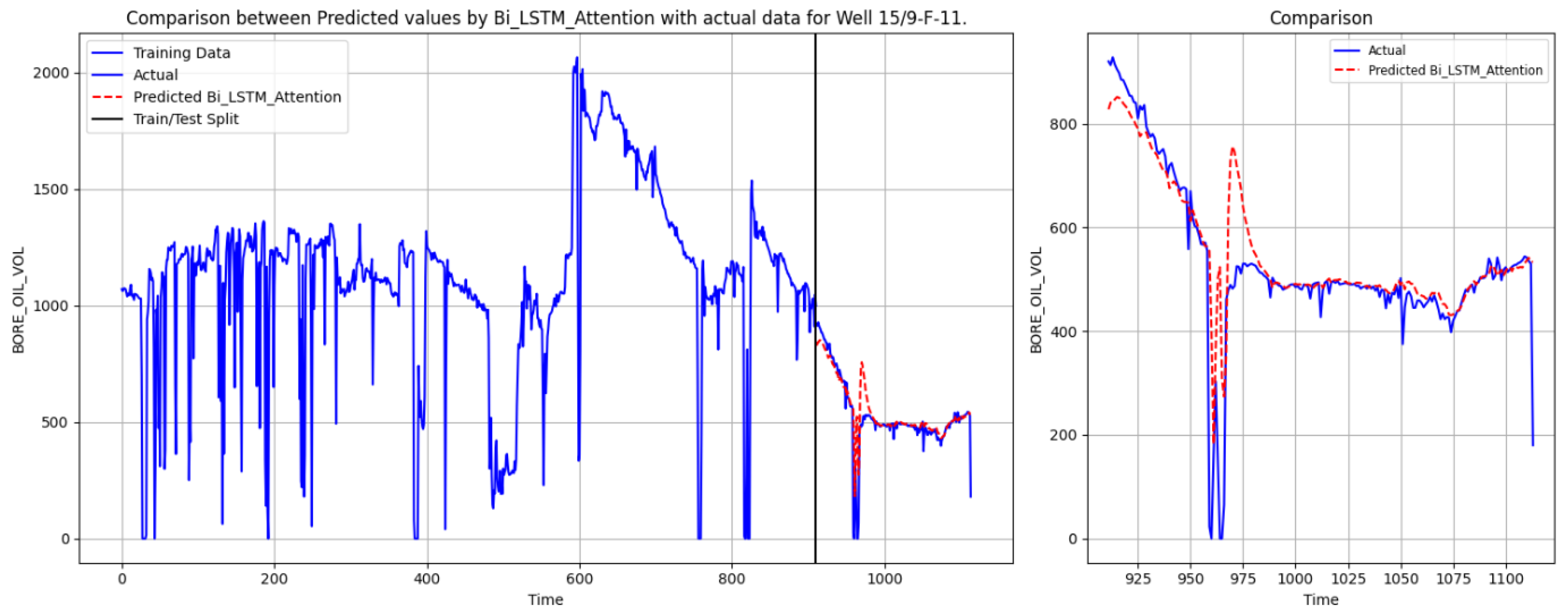Figure 8 illustrates the performance of Bi-LSTM-Attention, which more accurately follows the overall downward trend and demonstrates better adaptability at certain abrupt change points. Nevertheless, this model still exhibits deviations in predicting sudden short-term fluctuations, leading to noticeable discrepancies between predicted and actual values at specific moments. 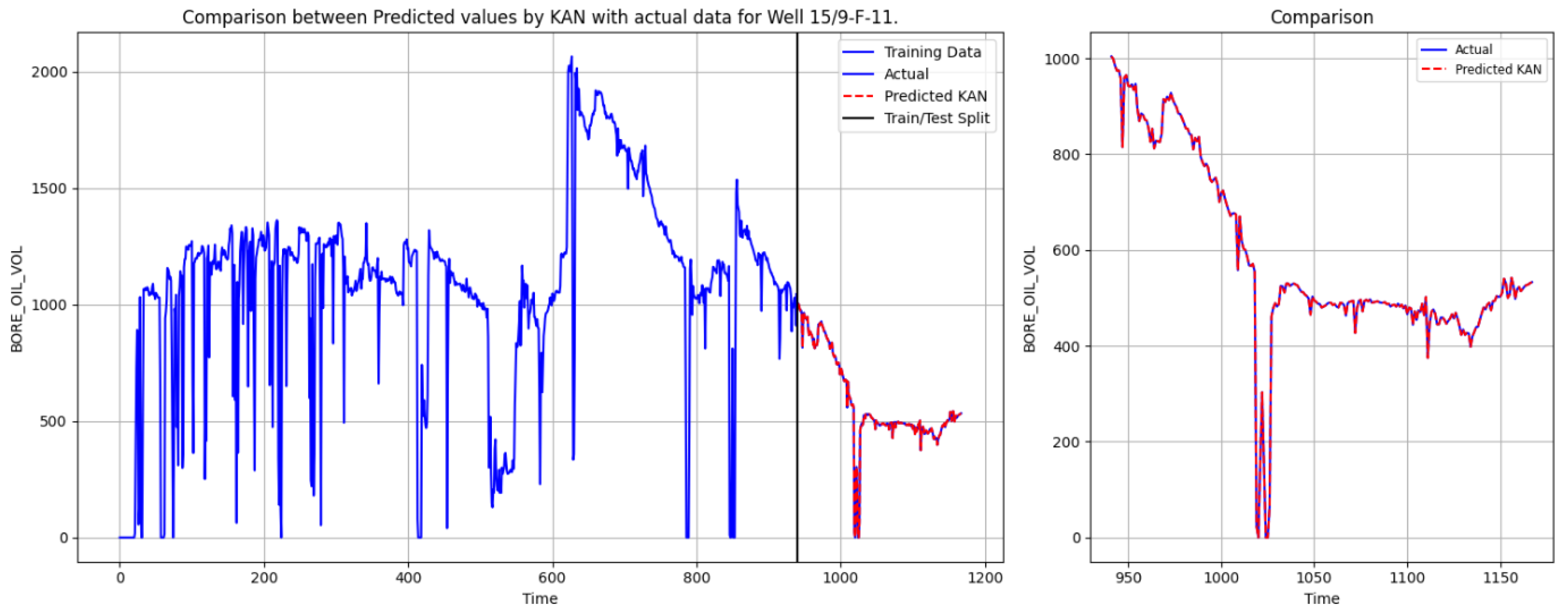Figure 9 displays the prediction results of the KAN model. Both in terms of overall trend and local details, the KAN’s predictions align closely with actual data, showing minimal overfitting and achieving high accuracy in capturing rapid transitions.

The comparative experimental results indicate that the SVR model performed relatively poorly, with significant deviations between the predicted values and the actual values. TFT effectively models long-term dependencies and integrates multiple temporal variables, yet it struggles with short-term abrupt changes, resulting in relatively smoothed predictions. Bi-LSTM-Attention enhances temporal resolution through attention mechanisms, improving short-term forecasting accuracy to some extent, but it still encounters difficulties in fully mitigating errors in sudden fluctuations. In contrast, the KAN, leveraging its powerful nonlinear modeling capability, achieves the best forecasting performance in this study. Its predicted trajectory closely aligns with the actual production curve, precisely capturing transition points. While maintaining high predictive accuracy, it effectively models complex temporal dynamics and demonstrates superior generalization performance among various deep learning architectures.

To verify the superiority of the KAN model, we also used the Well 15/9-F-14 data for oil production prediction. Figure 10, Figure 11, Figure 12 and Figure 13 show the oil production prediction for Well 15/9-F-14 by SVR, TFT, Bi-LSTM Attention, and the KAN.

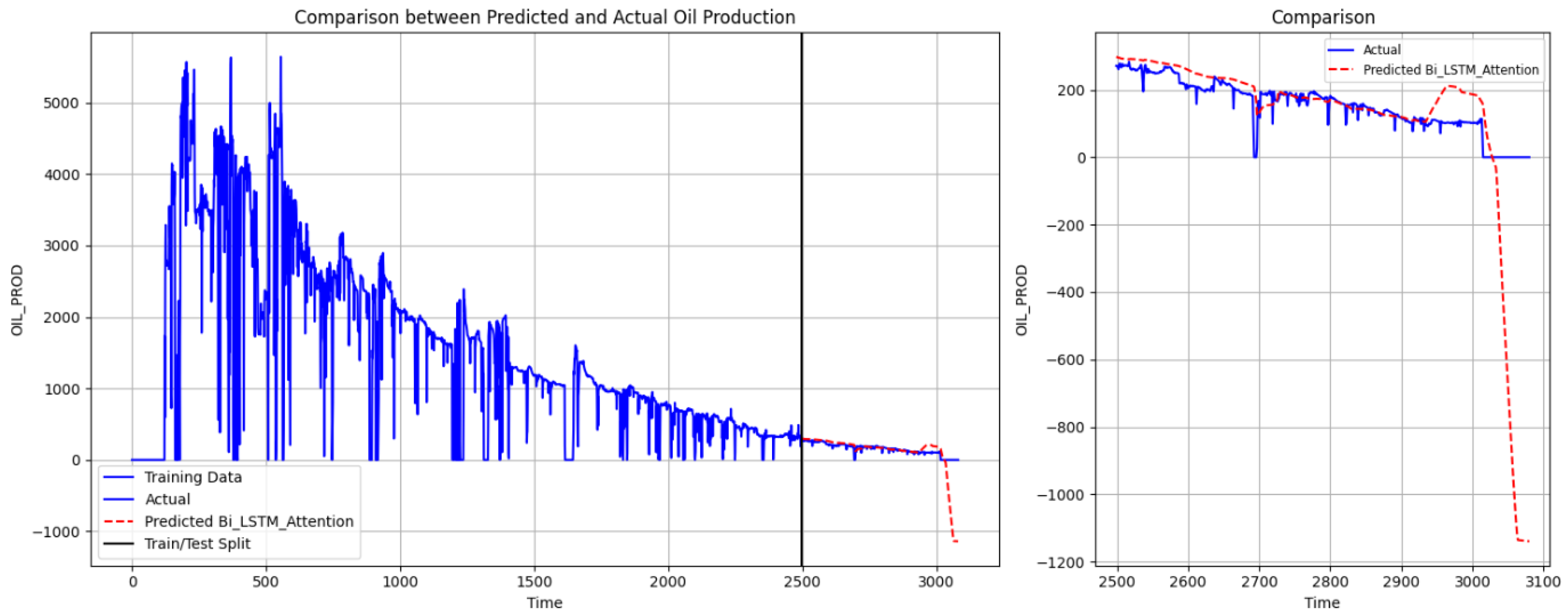
The SVR model performs the worst, with consistently high error values for both wells, reflecting its limited ability to fit complex data patterns. TFT struggles to accurately track actual values during sudden declines, leading to significant underestimation in the later test period. This indicates that TFT has certain limitations in handling abrupt changes and short-term volatility. Bi-LSTM-Attention improves short-term forecasting accuracy. However, in the latter part of the test period, it still fails to precisely predict sharp drops in oil production. In contrast, the KAN model demonstrates significantly higher prediction accuracy than SVR, TFT, and Bi-LSTM-Attention. It not only closely follows the actual production curve and captures long-term trends but also effectively adapts to sudden fluctuations.

These experimental results indicate that while TFT and Bi-LSTM-Attention provide reasonable predictions in stable regions compared to SVR, their accuracy declines significantly when faced with abrupt changes. This limitation stems from LSTM’s reliance on fixed-length memory units, which hinders its ability to adapt to sudden transitions. In contrast, the KAN treats transformations as continuous functions rather than relying on discrete matrix multiplications and nonlinear activations, as seen in traditional MLPs and LSTM. The KAN layer is structured as a learnable matrix of one-dimensional functions, offering a more flexible representation that enables it to capture complex temporal dependencies with fewer parameters and enhanced computational efficiency. Moreover, the KAN incorporates residual activation functions and dynamic grid refinement techniques, allowing it to continuously adjust its function approximation capability. This ensures that the model maintains a high degree of accuracy across both smooth and highly volatile regions.

To further quantify the predictive performance,

Table 9. Testing score comparison of all models for Well 15/9-F-11.

Error	SVR	TFT	Bi-LSTM Attention	KAN
MAE	89.7779	0.0588	0.0186	0.0040
RMSE	97.4335	0.0688	0.0428	0.0045

and

Table 10. Testing score comparison of all models for Well 15/9-F-14.

Error	SVR	TFT	Bi-LSTM Attention	KAN
MAE	94.6198	0.0225	0.0166	0.0033
RMSE	94.6516	0.0514	0.0450	0.0037

summarize the error metrics, including MAE and RMSE, for each model. These statistical measures provide a more comprehensive evaluation of accuracy, complementing the qualitative insights from the visual comparisons.

Overall, the SVR model is relatively traditional and lacks the sophistication and flexibility of some modern machine learning methods, making it unable to fully utilize the complexity and diversity of current data. For neural network models, while TFT effectively models long-term dependencies, it struggles to adapt to short-term variations, resulting in the highest errors. Bi-LSTM Attention improves prediction accuracy compared to TFT but still exhibits noticeable deviations when handling sharp production declines. The KAN achieves the lowest errors across both wells, with MAE and RMSE significantly lower than those of the other models.

These results demonstrate the excellent generalization performance of the KAN under both stable and highly volatile production conditions, making it the most effective model for oil production forecasting. Its superior ability to approximate complex nonlinear relationships and adapt to dynamic production fluctuations highlights its potential as a powerful time series forecasting tool in the energy sector.

6. Conclusions

In this study, we introduce the KAN as a novel deep learning framework for oil production prediction, using its powerful functional decomposition capability to model complex time-dependent and nonlinear relationships. Comparison experiments with SVR, TFT, and Bi-LSTM Attention show that the KAN significantly outperforms traditional sequence modeling methods. The lowest MAE and RMSE are achieved in multiple wells with minimal parameters, and the model is effective in capturing both long-term production trends and short-term fluctuations. Especially in regions with abrupt changes, the model’s robustness in dealing with dynamic production environments is highlighted. These results validate the effectiveness of the KAN’s adaptive spline-based activation function and function mapping structure, resulting in more accurate time series forecasts for the energy industry.

As an advanced time series forecasting framework, the KAN demonstrates exceptional accuracy, computational efficiency, and generalization capabilities in oil production prediction. The findings of this study further underscore the KAN’s potential as a powerful predictive tool in the energy sector, offering new opportunities for optimizing reservoir management and strategic planning.

Although the KAN has demonstrated excellent performance in oil production forecasting, certain limitations remain and warrant further investigation. The current study primarily relies on historical production data and does not explicitly incorporate key geological and engineering factors that play a crucial role in reservoir dynamics. This may limit the model’s ability to fully capture subsurface heterogeneity and the impact of operational activities. Parameters such as permeability, porosity, well pattern, and water/gas injection significantly influence production trends, and their integration could enhance prediction accuracy and model generalization. Future work will focus on incorporating these features to improve forecasting performance, making the KAN more adaptable to diverse reservoir conditions and further strengthening its potential in production optimization and decision support.