
Enhanced Short-Term PV Power Forecasting via a Hybrid Modified CEEMDAN-Jellyfish Search Optimized BiLSTM Model


Abstract
1. Introduction
- 1.
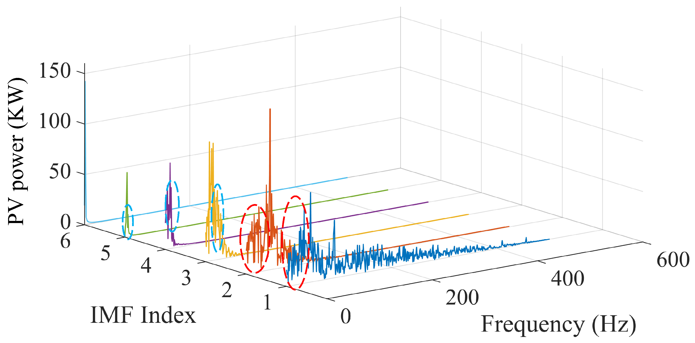
- The proposed method applies CEEMDAN for signal decomposition and FFT for extracting IMF frequency features. IPCC is introduced to cluster and reconstruct IMFs based on frequency similarity, enhancing input stability and clarity.
- 2.
- A BiLSTM-based predictor is developed, with hyperparameters efficiently optimized via the JS algorithm to improve accuracy and generalization while avoiding manual tuning pitfalls.
- 3.
- By combining CEEMDAN, IPCC, JS, and BiLSTM, the proposed hybrid framework effectively addresses nonlinearity, nonstationarity, and structural complexity in PV power forecasting.
2. Theory Ground
2.1. CEEMDAN Theory
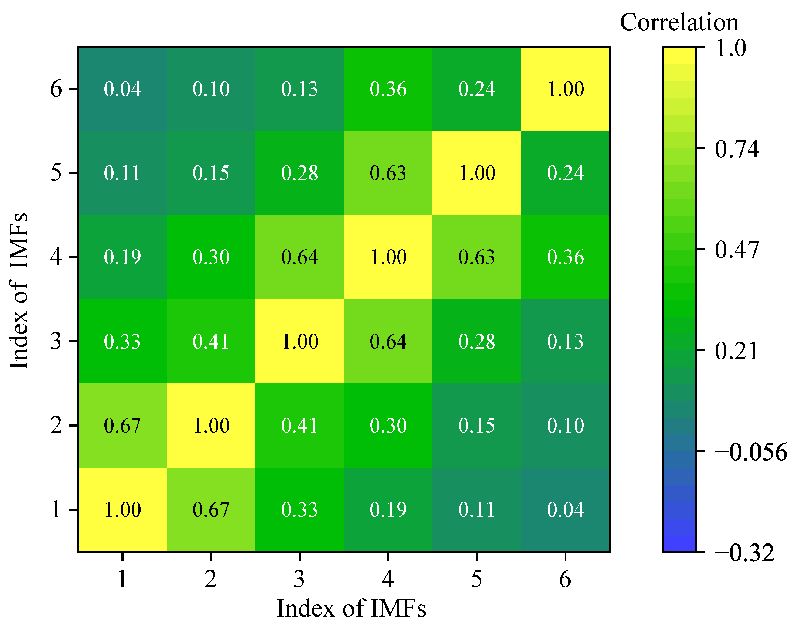
2.2. Improved Pearson Correlation Coefficient (IPCC)
2.2.1. Pearson Correlation Coefficient (PCC)
2.2.2. Improved Pearson Correlation Coefficient (IPCC)
2.3. Jellyfish Search Algorithm (JS)
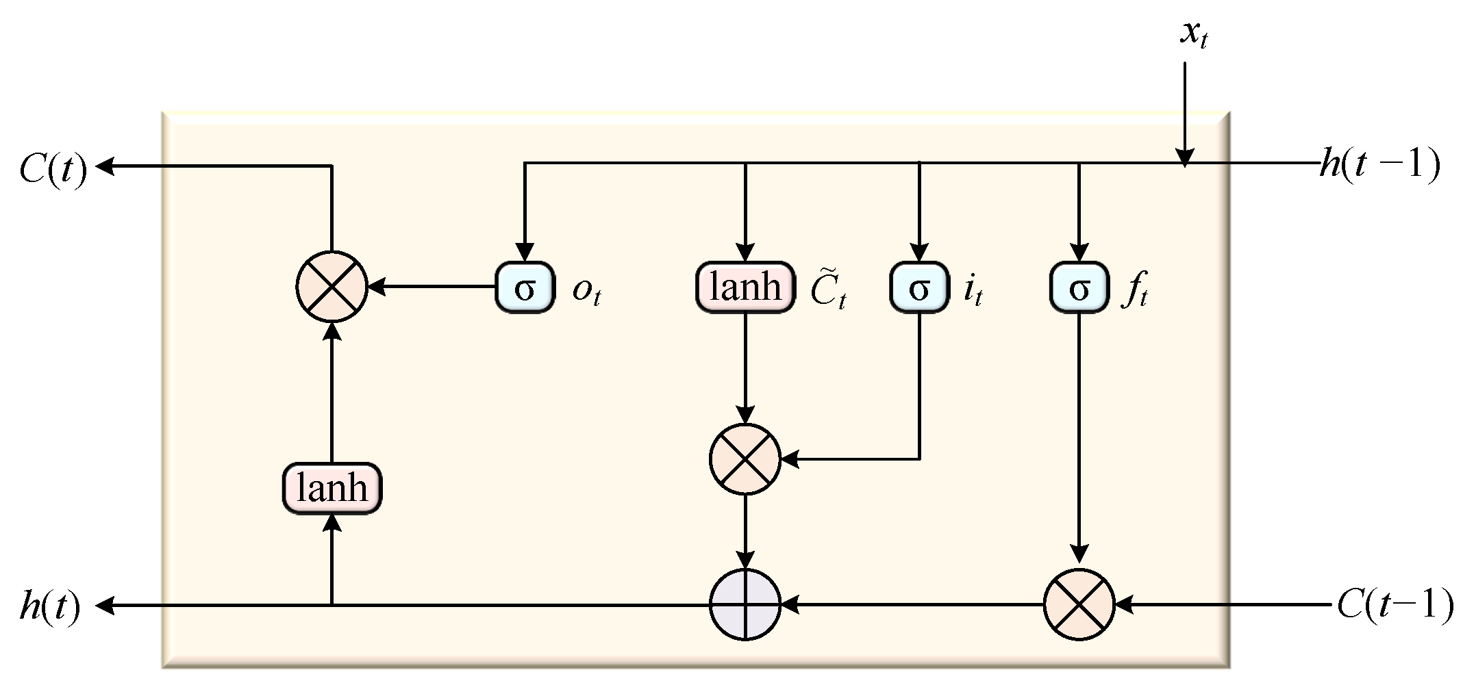
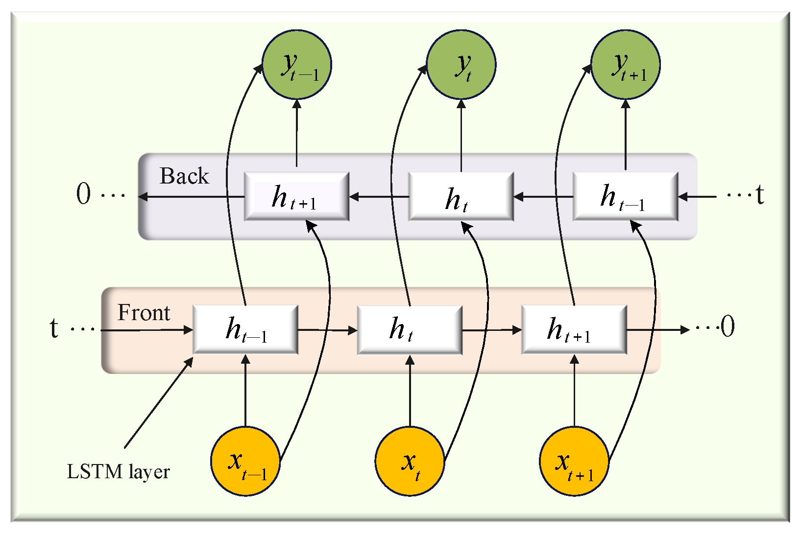
2.4. Bidirectional Long Short-Term Memory (BiLSTM)
3. Proposed Methodology
| Algorithm 1 Hybrid forecasting framework with CEEMDAN–JS–BiLSTM. |
|
3.1. Classification of the IMF Based on FFT and IPCC
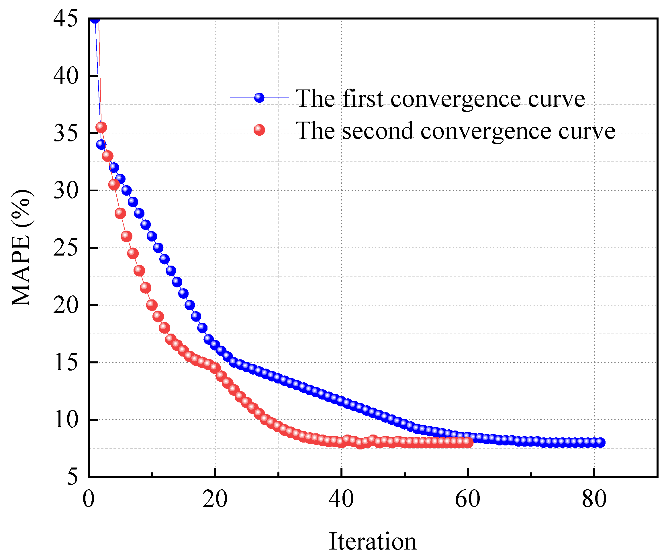
3.2. BiLSTM Optimization with JS
| Algorithm 2 JS optimization for BiLSTM hyperparameters. |
|
3.3. Prediction Results Evaluation
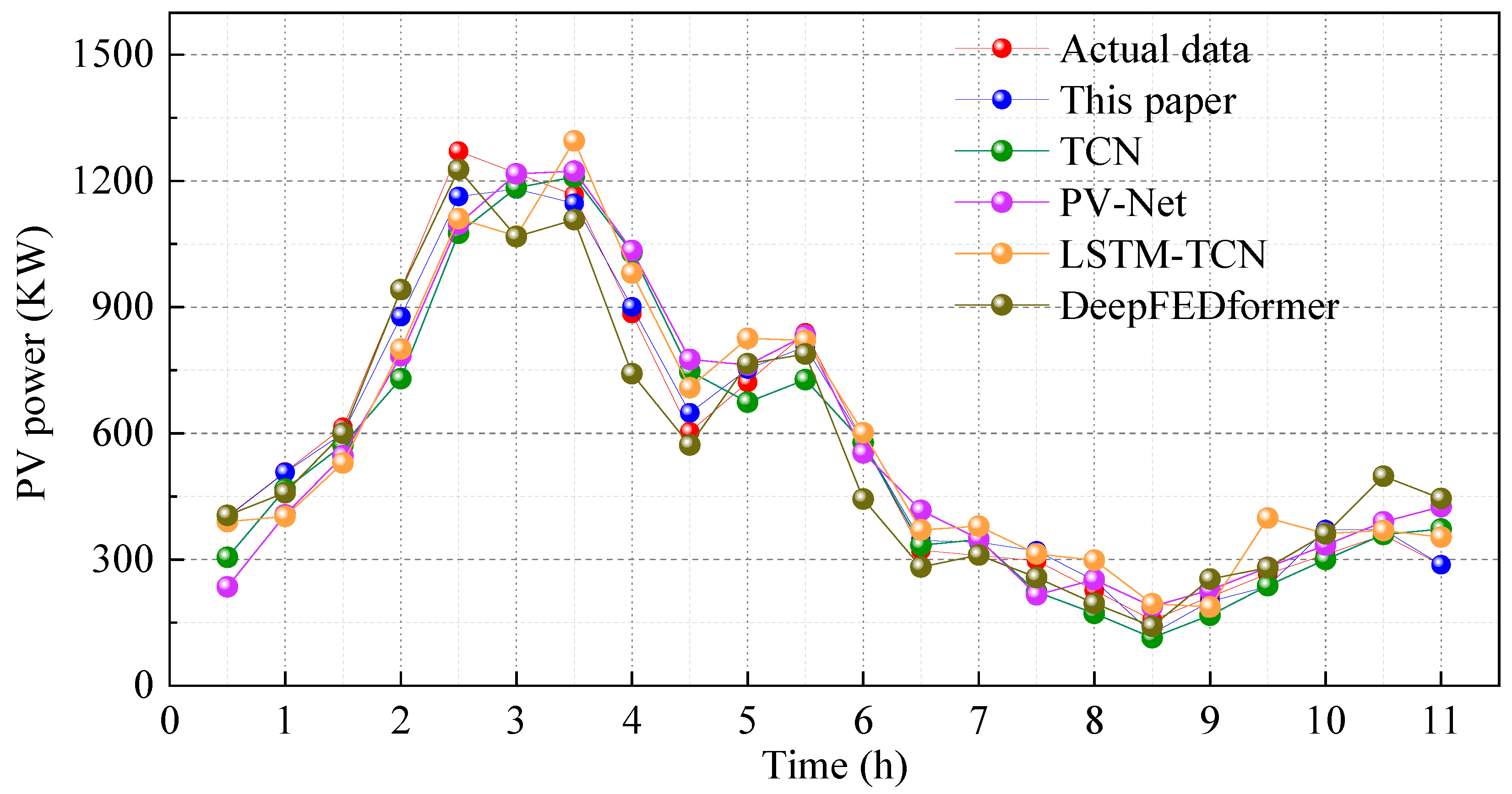
4. Result and Discussion
5. Conclusions
Author Contributions
Funding
Data Availability Statement
Acknowledgments
Conflicts of Interest
Abbreviations
| PV | Photovoltaic |
| LSTM | Long Short-Term Memory |
| CNN | Convolutional Neural Network |
| CEEMDAN | Complete Ensemble Empirical Mode Decomposition with Adaptive Noise |
| BiLSTM | Bidirectional Long Short-Term Memory |
| VMD | Variational Mode Decomposition |
| SSA | Singular Spectrum Analysis |
| PTFNet | Physically informed Temporal Fusion Network |
| EMD | Empirical Mode Decomposition |
| EEMD | Ensemble Empirical Mode Decomposition |
| CEEMD | Complete Ensemble Empirical Mode Decomposition |
| ITD | Intrinsic Time-scale Decomposition |
| UPITD | Uniform Phase Intrinsic Time-scale Decomposition |
| IMF | Intrinsic Mode Function |
| FFT | Fast Fourier Transform |
| IPCC | Inter-Component Phase Correlation Coefficient |
| JS | Jellyfish Search |
| PCC | Pearson Correlation Coefficient |
| IQR | Interquartile Range |
| NIMF | New of Intrinsic Mode Functions |
| RMSE | Root Mean Square Error |
| MAPE | Mean Absolute Percentage Error |
| TCN | Temporal Convolutional Network |
References
- Gu, B.; Shen, H.; Lei, X. Forecasting and uncertainty analysis of day-ahead photovoltaic power using a novel forecasting method. Appl. Energy 2021, 299, 117291. [Google Scholar] [CrossRef]
- Mayer, M.; Yang, D. Pairing ensemble numerical weather prediction with ensemble physical model chain for probabilistic photovoltaic power forecasting. Renew. Sustain. Energy Rev. 2023, 175, 113171. [Google Scholar] [CrossRef]
- Cui, S.; Lyu, S.; Ma, Y.; Wang, K. Improved informer PV power short-term prediction model based on weather typing and AHA-VMD-MPE. Energy 2024, 307, 132766. [Google Scholar] [CrossRef]
- Ling, H.; Liu, M.; Fang, Y. Deep Edge-Based Fault Detection for Solar Panels. Sensors 2024, 24, 5348. [Google Scholar] [CrossRef]
- Wang, Y.; Yao, Y.; Zou, Q.; Zhao, K.; Hao, Y. Forecasting a Short-Term Photovoltaic Power Model Based on Improved Snake Optimization, Convolutional Neural Network, and Bidirectional Long Short-Term Memory Network. Sensors 2024, 24, 3897. [Google Scholar] [CrossRef]
- Joseph, L.P.; Deo, R.C.; Prasad, R.; Salcedo-Sanz, S.; Raj, N.; Soar, J. Near real-time wind speed forecast model with bidirectional LSTM networks. Renew. Energy 2023, 204, 39–58. [Google Scholar] [CrossRef]
- Li, S.; Ma, W.; Liu, Z.; Duan, Y.; Tian, C. Short-Term Prediction of Wind Power Based on NWP Error Correction with Time GAN and LSTM-TCN. In Energy Power and Automation Engineering; Springer: Singapore, 2024; pp. 939–948. [Google Scholar]
- Wang, L.; Mao, M.; Xie, J.; Liao, Z.; Zhang, H.; Li, H. Accurate solar PV power prediction interval method based on frequency-domain decomposition and LSTM model. Energy 2023, 262, 125592. [Google Scholar] [CrossRef]
- Khan, Z.A.; Hussain, T.; Baik, S.W. Dual stream network with attention mechanism for photovoltaic power forecasting. Appl. Energy 2023, 338, 120916. [Google Scholar] [CrossRef]
- Rai, A.; Shrivastava, A.; Jana, K.C. Differential attention net: Multi-directed differential attention based hybrid deep learning model for solar power forecasting. Energy 2023, 263, 125746. [Google Scholar] [CrossRef]
- Wolff, B.; Kühnert, J.; Lorenz, E.; Kramer, O.; Heinemann, D. Comparing support vector regression for PV power forecasting to a physical modeling approach using measurement, numerical weather prediction, and cloud motion data. Solar Energy 2016, 135, 197–208. [Google Scholar] [CrossRef]
- Brabec, M.; Pelikán, E.; Krc, P.; Eben, K.; Musilek, P. Statistical modeling of energy production by photovoltaic farms. In Proceedings of the Electric Power and Energy Conference (EPEC), Halifax, NS, Canada, 25–27 August 2010; IEEE: Piscataway, NJ, USA, 2010; pp. 1–6. [Google Scholar]
- Markovics, D.; Martin, J. Comparison of machine learning methods for photovoltaic power forecasting based on numerical weather prediction. Renew. Sustain. Energy Rev. 2022, 161, 112364. [Google Scholar] [CrossRef]
- Yang, D.; Dong, Z. Operational photovoltaics power forecasting using seasonal time series ensemble. Solar Energy 2018, 166, 529–541. [Google Scholar] [CrossRef]
- Qian, W.; Sui, A. A novel structural adaptive discrete grey prediction model and its application in forecasting renewable energy generation. Expert Syst. Appl. 2021, 186, 115761. [Google Scholar] [CrossRef]
- Douiri, M.R. Particle swarm optimized neuro-fuzzy system for photovoltaic power forecasting model. Solar Energy 2019, 184, 91–104. [Google Scholar] [CrossRef]
- Akhter, M.N.; Mekhilef, S.; Mokhlis, H.; Almohaimeed, Z.M.; Muhammad, M.A.; Khairuddin, A.S.M.; Akram, R.; Hussain, M.M. An hour-ahead PV power forecasting method based on an RNN-LSTM model for three different PV plants. Energies 2022, 15, 2243. [Google Scholar] [CrossRef]
- Li, G.; Guo, S.; Li, X.; Cheng, C. Short-term Forecasting Approach Based on bidirectional long short-term memory and convolutional neural network for Regional Photovoltaic Power Plants. Sustain. Energy Grids Netw. 2023, 34, 101019. [Google Scholar] [CrossRef]
- Chen, Z.R.; Bai, Y.L.; Hong, J.T. Constructing two-stream input matrices in a convolutional neural network for photovoltaic power prediction. Eng. Appl. Artif. Intell. 2024, 135, 108814. [Google Scholar] [CrossRef]
- Liu, Q.; Li, Y.; Jiang, H.; Chen, Y.; Zhang, J. Short-term photovoltaic power forecasting based on multiple mode decomposition and parallel bidirectional long short term combined with convolutional neural networks. Energy 2024, 286. [Google Scholar] [CrossRef]
- Xue, H.; Ma, J.; Zhang, J.; Jin, P.; Wu, J.; Du, F. Power Forecasting for Photovoltaic Microgrid Based on MultiScale CNN-LSTM Network Models. Energies 2024, 17, 3877. [Google Scholar] [CrossRef]
- Yu, J.; Li, X.; Yang, L.; Li, L.; Huang, Z.; Shen, K.; Yang, X.; Yang, X.; Xu, Z.; Zhang, D.; et al. Deep Learning Models for PV Power Forecasting. Energies 2024, 17, 3973. [Google Scholar] [CrossRef]
- Wang, S.; Huang, Y. Spatio-temporal photovoltaic prediction via a convolutional based hybrid network. Comput. Electr. Eng. 2025, 123, 110021. [Google Scholar] [CrossRef]
- Liang, J.; Yin, L.; Xin, Y.; Li, S.; Zhao, Y.; Song, T. Short-term photovoltaic power prediction based on CEEMDAN-PE and BiLSTM neural network. Electr. Power Syst. Res. 2025, 246, 111706. [Google Scholar] [CrossRef]
- Hosseini, E.; Saeedpour, B.; Banaei, M.; Ebrahimy, R. Optimized deep neural network architectures for energy consumption and PV production forecasting. Energy Strategy Rev. 2025, 59, 101704. [Google Scholar] [CrossRef]
- Bai, M.; Zhou, G.; Yao, P.; Dong, F.; Chen, Y.; Zhou, Z.; Yang, X.; Liu, J.; Yu, D. Deep multi-attribute spatial-temporal graph convolutional recurrent neural network-based multivariable spatial-temporal information fusion for short-term probabilistic forecast of multi-site photovoltaic power. Expert Syst. Appl. 2025, 279, 127458. [Google Scholar] [CrossRef]
- Zhai, C.; He, X.; Cao, Z.; Abdou-Tankari, M.; Wang, Y.; Zhang, M. Photovoltaic power forecasting based on VMD-SSA-Transformer: Multidimensional analysis of dataset length, weather mutation and forecast accuracy. Energy 2025, 324, 135971. [Google Scholar] [CrossRef]
- Piantadosi, G.; Dutto, S.; Galli, A.; De Vito, S.; Sansone, C.; Di Francia, G. Photovoltaic power forecasting: A Transformer based framework. Energy AI 2024, 18, 100444. [Google Scholar] [CrossRef]
- Tao, K.; Zhao, J.; Tao, Y.; Qi, Q.; Tian, Y. Operational day-ahead photovoltaic power forecasting based on transformer variant. Appl. Energy 2024, 373, 123825. [Google Scholar] [CrossRef]
- Qu, Z.; Hou, X.; Li, J.; Hu, W. Short-term wind farm cluster power prediction based on dual feature extraction and quadratic decomposition aggregation. Energy 2024, 290, 130155. [Google Scholar] [CrossRef]
- Xie, T.; Zhang, G.; Liu, H.; Liu, F.; Du, P. A hybrid forecasting method for solar output power based on variational mode decomposition, deep belief networks and autoregressive moving average. Appl. Sci. 2018, 8, 1901. [Google Scholar] [CrossRef]
- Khelifi, R.; Guermoui, M.; Rabehi, A.; Taallah, A.; Zoukel, A.; Ghoneim, S.S.; Bajaj, M.; AboRas, K.M.; Zaitsev, I. Short-Term PV Power Forecasting Using a Hybrid TVF-EMD-ELM Strategy. Int. Trans. Electr. Energy Syst. 2023, 2023, 6413716. [Google Scholar] [CrossRef]
- Wu, S.; Guo, H.; Zhang, X.; Wang, F. Short-Term Photovoltaic Power Prediction Based on CEEMDAN and Hybrid Neural Networks. IEEE J. Photovoltaics 2024, 14, 960–969. [Google Scholar] [CrossRef]
- Feng, H.; Yu, C. A novel hybrid model for short-term prediction of PV power based on KS-CEEMDAN-SE-LSTM. Renew. Energy Focus 2023, 47, 100497. [Google Scholar] [CrossRef]
- Wang, L.; Liu, Y.; Li, T.; Xie, X.; Chang, C. Short-term PV power prediction based on optimized VMD and LSTM. IEEE Access 2020, 8, 165849–165862. [Google Scholar] [CrossRef]
- Jodaei, A.; Moravej, Z.; Pazoki, M. Effective protection scheme for transmission lines connected to large scale photovoltaic power plants. Electr. Power Syst. Res. 2024, 228, 110103. [Google Scholar] [CrossRef]
- Ma, J.; Bai, X.; Ma, F.; Zhuo, S.; Sun, B.; Li, C. Convolutional Neural Network Design Based on Weak Magnetic Signals and Its Application in Aircraft Bearing Fault Diagnosis. IEEE Sensors J. 2024, 24, 36031–36043. [Google Scholar] [CrossRef]
- Jiang, Y.; Zheng, L.; Ding, X. Ultra-short-term prediction of photovoltaic output based on an LSTM-ARMA combined model driven by EEMD. J. Renew. Sustain. Energy 2021, 13, 046103. [Google Scholar] [CrossRef]
- Huang, Y.; Liu, J.; Zhang, Z.; Li, D.; Li, X.; Wang, G. Dynamic Combination Forecasting for Short-Term Photovoltaic Power. IEEE Trans. Artif. Intell. 2024, 5, 5277–5289. [Google Scholar] [CrossRef]
- Sareen, K.; Panigrahi, B.K.; Shikhola, T. A short-term solar irradiance forecasting modelling approach based on three decomposition algorithms and adaptive neuro-fuzzy inference system. Expert Syst. Appl. 2023, 231, 120770. [Google Scholar] [CrossRef]
- Li, S.; Wang, J.; Zhang, H.; Liang, Y. Solar photovoltaic power forecasting system with online manner based on adaptive mode decomposition and multi-objective optimization. Comput. Electr. Eng. 2024, 118, 109407. [Google Scholar] [CrossRef]
- Zhang, D.; Chen, B.; Zhu, H.; Goh, H.H.; Dong, Y.; Wu, T. Short-term wind power prediction based on two-layer decomposition and BiTCN-BiLSTM-attention model. Energy 2023, 285, 128762. [Google Scholar] [CrossRef]
- Agga, A.; Abbou, A.; Labbadi, M.; El Houm, Y.; Ali, I.H.O. CNN-LSTM: An efficient hybrid deep learning architecture for predicting short-term photovoltaic power production. Electr. Power Syst. Res. 2022, 208, 107908. [Google Scholar] [CrossRef]
- Li, N.; Li, L.; Zhang, F.; Jiao, T.; Wang, S.; Liu, X.; Wu, X. Research on short-term photovoltaic power prediction based on multi-scale similar days and ESN-KELM dual core prediction model. Energy 2023, 277, 127557. [Google Scholar] [CrossRef]
- Yang, X.; Wang, S.; Peng, Y.; Chen, J.; Meng, L. Short-term photovoltaic power prediction with similar-day integrated by BP-AdaBoost based on the Grey-Markov model. Electr. Power Syst. Res. 2023, 215, 108966. [Google Scholar] [CrossRef]
- Liu, Y.; Zuo, H.; Liu, Z.; Fu, Y.; Jia, J.J.; Dhupia, J.S. Electrostatic signal self-adaptive denoising method combined with CEEMDAN and wavelet threshold. Aerospace 2024, 11, 491. [Google Scholar] [CrossRef]
- Gong, J.; Qu, Z.; Zhu, Z.; Xu, H. Parallel TimesNet-BiLSTM model for ultra-short-term photovoltaic power forecasting using STL decomposition and auto-tuning. Energy 2025, 320, 135286. [Google Scholar] [CrossRef]
- Chou, J.S.; Truong, D.N. A novel metaheuristic optimizer inspired by behavior of jellyfish in ocean. Appl. Math. Comput. 2021, 389, 125535. [Google Scholar] [CrossRef]
- Li, Y.; Song, L.; Zhang, S.; Kraus, L.; Adcox, T.; Willardson, R.; Komandur, A.; Lu, N. A TCN-based hybrid forecasting framework for hours-ahead utility-scale PV forecasting. IEEE Trans. Smart Grid 2023, 14, 4073–4085. [Google Scholar] [CrossRef]
- Abdel-Basset, M.; Hawash, H.; Chakrabortty, R.K.; Ryan, M. PV-Net: An innovative deep learning approach for efficient forecasting of short-term photovoltaic energy production. J. Clean. Prod. 2021, 303, 127037. [Google Scholar] [CrossRef]
- Limouni, T.; Yaagoubi, R.; Bouziane, K.; Guissi, K.; Baali, E.H. Accurate one step and multistep forecasting of very short-term PV power using LSTM-TCN model. Renew. Energy 2023, 205, 1010–1024. [Google Scholar] [CrossRef]
- Wen, Y.; Pan, S.; Li, X.; Li, Z.; Wen, W. Improving multi-site photovoltaic forecasting with relevance amplification: DeepFEDformer-based approach. Energy 2024, 299, 131479. [Google Scholar] [CrossRef]


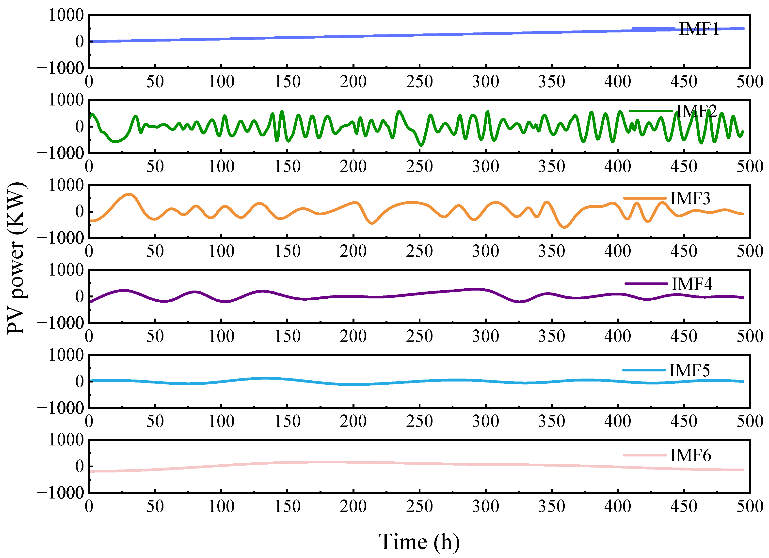
| IMF Pair | IPCC Value | Correlation |
|---|---|---|
| IMF1 and IMF2 | 0.67 | High |
| IMF2 and IMF3 | 0.41 | Low |
| IMF3 and IMF4 | 0.64 | High |
| IMF4 and IMF5 | 0.63 | High |
| IMF5 and IMF6 | 0.24 | Low |
| Model | RMSE | MAPE (%) | |
|---|---|---|---|
| BiLSTM | 104.8925 | 16.9725 | 0.9032 |
| CEEMDAN-BiLSTM | 76.3219 | 13.4378 | 0.9433 |
| JS-BiLSTM | 87.4532 | 14.7441 | 0.9265 |
| CEEMDAN-Grouped BiLSTM | 46.4325 | 10.2461 | 0.9673 |
| CEEMDAN–JS–BiLSTM | 37.2833 | 8.1231 | 0.9785 |
Disclaimer/Publisher’s Note: The statements, opinions and data contained in all publications are solely those of the individual author(s) and contributor(s) and not of MDPI and/or the editor(s). MDPI and/or the editor(s) disclaim responsibility for any injury to people or property resulting from any ideas, methods, instructions or products referred to in the content. |
© 2025 by the authors. Licensee MDPI, Basel, Switzerland. This article is an open access article distributed under the terms and conditions of the Creative Commons Attribution (CC BY) license (https://creativecommons.org/licenses/by/4.0/).
Share and Cite
Liu, Y.; Wang, J.; Song, L.; Liu, Y.; Shen, L. Enhanced Short-Term PV Power Forecasting via a Hybrid Modified CEEMDAN-Jellyfish Search Optimized BiLSTM Model. Energies 2025, 18, 3581. https://doi.org/10.3390/en18133581
Liu Y, Wang J, Song L, Liu Y, Shen L. Enhanced Short-Term PV Power Forecasting via a Hybrid Modified CEEMDAN-Jellyfish Search Optimized BiLSTM Model. Energies. 2025; 18(13):3581. https://doi.org/10.3390/en18133581
Chicago/Turabian StyleLiu, Yanhui, Jiulong Wang, Lingyun Song, Yicheng Liu, and Liqun Shen. 2025. "Enhanced Short-Term PV Power Forecasting via a Hybrid Modified CEEMDAN-Jellyfish Search Optimized BiLSTM Model" Energies 18, no. 13: 3581. https://doi.org/10.3390/en18133581
APA StyleLiu, Y., Wang, J., Song, L., Liu, Y., & Shen, L. (2025). Enhanced Short-Term PV Power Forecasting via a Hybrid Modified CEEMDAN-Jellyfish Search Optimized BiLSTM Model. Energies, 18(13), 3581. https://doi.org/10.3390/en18133581