Assessment of Building Compactness at Initial Design Stage of Single-Family Houses

Abstract

The paper is the culmination of research on geometric aspects of assessing the energy demand of a single-family house. In a recent study, two collections of single-family houses were analyzed: (a) a collection of 21 with outlines assumed a priori so that the building area was constant (which is not achievable in practice) and (b) a collection of 33 real buildings, recently designed by the Polish design studio Galeria Domów. These examples show the functioning of the indicators analyzed by the author in earlier papers and indicate the ${RC}_{sq}$ indicator that best reflects the assessment of building compactness in percentage points in relation to the ideal shape of the building plan, which is a square. The ${RC}_{sq}$ index is economically expressed by only two parameters, namely the base area ${\mathrm{A}}_{\mathrm{f}}$ and the building outline perimeter $\mathrm{P}$, and therefore is easy to implement in the BIM system and at the same time covers high-rise buildings. As it turned out, the tested buildings from Galeria Domów have very good geometric and therefore energy efficiency. The above-mentioned indicator also highlights the advisability of analyzing the heated part in addition to the standard full-contour analyses.

1. Introduction

Residential houses constitute an important sector in the environment as they provide essential living space, but are also responsible for a significant part of final energy consumption. Buildings that were constructed to outdated standards generally struggle to meet current energy efficiency standards. In particular, in Europe, as many as 35% of buildings were built more than fifty years ago [1]. In order to formulate a thermal modernization plan, an important issue is the overall assessment of the geometry of buildings in a given area. To investigate the geometry of buildings in larger built-up areas, an important role may be played by the automatic installed measurement system proposed in [1]. Optimization studies in the field of geometry using genetic algorithms can be found in [2], in the field of roof shaping and the use of the so-called Trombe wall in [3], and a discussion on increasing energy efficiency by developing the building surroundings can be found in [4]. Building prototyping can play an important role in investigating the structure of building geometry, which can then be used in the analysis of energy demand according to statistically feasible models [5]. The novelty of this research involves a hybrid approach combining stratified sampling and k-means clustering to establish prototypes of building geometry. In the paper [6], based on this approach, nine prototypes of building geometry were identified and modeled. These statistically representative prototypes provide information about the building geometry and feature-based assessments are used for subsequent energy demand analysis. There is ongoing research into the impact of the form factor (however defined) on the total heating and cooling energy consumption of a building [7,8,9,10]. The total amount of energy needed to heat and cool a building can be calculated using dynamic modeling using EnergyPlus v.9.3.0 software [11]. For simulation purposes, models of residential buildings with a passive solar area and square and rectangular floors were designed [6]. Even in high-rise buildings, the geometry of courtyards and balconies can be used for natural ventilation, thus reducing energy consumption [12]. Among the latest articles in the literature, we can find papers on the relationship between the energy efficiency of a building and the geometry of its shape. Optimizing building form and design variables early in the architectural design process, particularly in the conceptual phase, can significantly improve overall design performance and energy efficiency at minimal cost. In particular, “compactness”, which is a geometric sub-concept of building form, is one of the most important factors in terms of heat loss and gain of a building [13]. We can also read about the advisability of analyzing energy demand in the early stages of designing a residential building in terms of its geometric features in the paper [14]. Optimizing building form and design variables early in the architectural design process, particularly in the conceptual phase, can significantly improve the overall design’s geometric performance and energy efficiency at minimal cost. Proposals for energy optimization of buildings, among others, with regard to geometry can also be found in the paper [15].

The studies conducted so far, both those conducted a long time ago and those conducted currently, using various geometric compactness indices—nominative [16,17], non-nomative [18], and relative [19,20,21,22,23,24,25]—do not provide universal, simple methods of evaluation, e.g., in percentage points. This paper is a direct continuation and summary of the articles [26,27,28] in the field focused on optimizing the shape of a building with respect to the amount of energy consumption, both built-in and operational [7,8,9,10], and on what should be particularly emphasized; this paper presents an indicator expressing percentage geometric energy efficiency, not previously found in the literature. According to the author, this paper also concludes the discussion, conducted in [26,27,28], on the use of shape indicators at the stage of designing single-family houses in the BIM concept [29]. The rapidly developing BIM technology was initiated by Eastman in [30], in which he described a computer program capable of performing parametric design and 3D representation of an object. Nowadays, it is a well-established theory, deeply rooted in practice, as evidenced by the reissued books containing a compendium of knowledge in the field of design using BIM. The use of geometric indicators proposed in [26,27,28], which are easy to determine, is perfectly suited for use in BIM software.

Among many factors influencing the demand for built-in energy in single-family houses, the geometric factor, i.e., the shape, is undoubtedly important [27].

2. Computational Data, Methods and Objectives

The papers [27,28] show strong relationships between material consumption (embodied energy [7,8,9,10]) and the corresponding indicators (${RC}_{cube}$, ${RC}_{cd}$, ${RC}_{sq}$, $A/V$, $EWA/FA$) [27] and between energy demand (functional energy [7,8,9,10]) [29] and the above-mentioned indicators. Let us recall the definitions of these indicators.

Assuming that ${\mathrm{A}}_{\mathrm{f}}$ is the area of the plan of a house, $\mathrm{P}$ is the perimeter of the plan of a house, and h is the height of the external wall, we define:

$$EWA/FA={\displaystyle \frac{\mathrm{Ph}}{{\mathrm{A}}_{\mathrm{f}}}}$$

(1)

then expressing the ratio of external wall area to floor area;

$${RC}_{cube}={\displaystyle \frac{2{\mathrm{A}}_{\mathrm{f}}+\mathrm{P}\mathrm{h}}{6{\left({\mathrm{A}}_{\mathrm{f}}\mathrm{h}\right)}^{\frac{2}{3}}}} ,$$

(2)

which is the relative compactness indicator with respect to a cube;

$${RC}_{cd}={\displaystyle \frac{2{\mathrm{A}}_{\mathrm{f}}+\mathrm{Ph}}{2{\mathrm{A}}_{\mathrm{f}}+4\sqrt{{\mathrm{A}}_{\mathrm{f}}}\mathrm{h}}} ,$$

(3)

which is the relative compactness indicator with respect to a cuboid;

$${RC}_{sq}={\displaystyle \frac{\mathrm{P}}{4\sqrt{{\mathrm{A}}_{\mathrm{f}}}}},$$

(4)

which is the planar relative compactness indicator with respect to a square, the main indicator in this paper;

$$A/V={\displaystyle \frac{\mathrm{P}\mathrm{h}+2{\mathrm{A}}_{\mathrm{f}}}{{\mathrm{A}}_{\mathrm{f}}·\mathrm{h}}},$$

(5)

which is the ratio of total area and volume, and finally

$$LBI={\displaystyle \frac{\mathrm{P}+\sqrt{{\mathrm{P}}^2-16{\mathrm{A}}_{\mathrm{f}}}}{\mathrm{P}-\sqrt{{\mathrm{P}}^2-16{\mathrm{A}}_{\mathrm{f}}}}} ,$$

(6)

which is the ratio of two sides of a rectangle with area ${\mathrm{A}}_{\mathrm{f}}$ and perimeter $\mathrm{P}$ [27,28].

This study focuses on the geometric efficiency assessment method based on the results of [27,28], which proved a strong correlation between the indicator values and both types of energy: embodied and functional.

As we said above, the indicator (4) will be the key parameter proposed to characterize the optimal geometric compactness of buildings.

Let us analyze the geometric essence of the indicator (4) in more detail. Let us multiply the numerator and denominator of the fraction (4) by the height $\mathrm{h}$. Then we obtain a relationship of the form ${RC}_{sq}$ = ${\displaystyle \frac{\mathrm{P}\mathrm{h}}{4\sqrt{{\mathrm{A}}_{\mathrm{f}}}\mathrm{h}}}$. Then in the numerator we have the area of the external walls of the analyzed building, while in the denominator, we have the area of the external walls of a building with the same base area ${\mathrm{A}}_{\mathrm{f}}$, but in the shape of a square, i.e., the reference building with a square base. After multiplying by 100% we obtain the percentage deviation of the surface of the external walls of a given building from the reference building. The indicator (4) becomes a sensational parameter in its geometric essence and computational simplicity, characterizing the shape of the building, and such an interpretation has not been encountered in the literature so far. Taking into account mainly the indicator (4), we will formulate the (multi-aspect) goal of the work.

The aim of the paper is to (O1) demonstrate the correlation between indices (1)–(6) in relation to buildings with shapes assumed a priori; (O2) check the functioning of indices (1)–(6) with particular emphasis on index (4) on data from real projects; (O3) determine, using indicator (4), the percentage deviations of the external wall surface from the reference (ideal) value with an indication of its application at an early stage of design. The result of the research is also an answer to the following question: what is the geometric compactness of currently designed single-family houses?

We will also formulate and prove through further calculations and analyses the following thesis: without limiting the designers’ creative inventiveness, it is possible to design a house in such a way as to achieve high geometric efficiency by checking the value of the index (4) already at the initial design stage.

Let us note at the outset that the search for the optimal geometric shape of a building does not in any way limit the necessary continuous research towards optimizing the demand for both built-in and functional energy. Optimizing the geometric shape of a building is, as it were, above all concepts of energy acquisition. It does not depend on the climatic region in which the building is located.

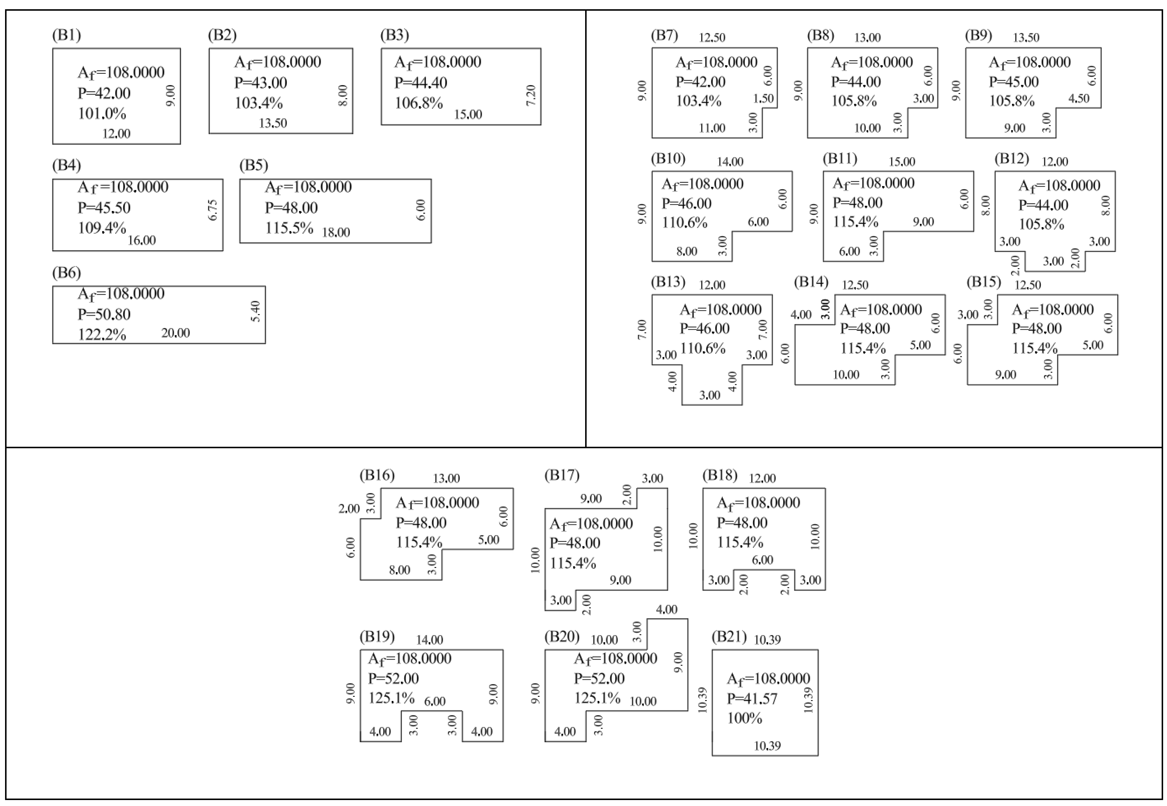
We accept two collections of building designs for analysis of their plans (floor plans). The first collection is defined a priori by arbitrarily assuming (as outlines of building projections) 21 different rectangular polygons [27] with a constant surface area of exactly 108 [m²] (see

Table 1. (a) Basic geometrical parameters and indicators of the buildings B1–B11. (b) Basic geometrical parameters and indicators of the buildings B12–B21.

(a)
Parameter	Unit	Building Number
		B1	B2	B3	B4		B5		B6		B7		B8		B9		B10		B11
Af	m2	108	108	108	108		108		108		108		108		108		108		108
P	m	42.00	43.00	44.40	45.50		48.00		50.80		43.00		44.00		45.00		46.00		48.00
h	m	3.00	3.00	3.00	3.00		3.00		3.00		3.00		3.00		3.00		3.00		3.00
RCcube	-	1.208	1.219	1.234	1.245		1.272		1.302		1.219		1.230		1.240		1.251		1.272
RCcd	-	1.004	1.013	1.025	1.035		1.057		1.081		1.013		1.021		1.030		1.039		1.057
LBI	-	1.333	1.688	2.083	2.370		3.000		3.704		1.688		1.975		2.241		2.498		3.000
EWA/FA	-	1.167	1.194	1.233	1.264		1.333		1.411		1.194		1.222		1.250		1.278		1.333
A/V	m−1	1.056	1.065	1.078	1.088		1.111		1.137		1.065		1.074		1.083		1.093		1.111
RCsq	-	1.010	1.034	1.068	1.094		1.155		1.222		1.034		1.058		1.082		1.106		1.154
Csq	%	101	103.4	106.8	109.4		115.5		122.2		103.4		105.8		108.2		110.6		115.4
(b)
Parameter	Unit	Building Number
		B12	B13	B14	B15		B16		B17			B18			B19		B20		B21
Af	m2	108	108	108	108		108		108			108			108		108		108
P	m	44.00	46.00	48.00	48.00		48.00		48.00			48.00			52.00		52.00		41.57
h	m	3.00	3.00	3.00	3.00		3.00		3.00			3.00			3.00		3.00		3.00
RCcube	-	1.230	1.251	1.272	1.272		1.272		1.272			1.272			1.314		1.314		1.204
RCcd	-	1.021	1.039	1.057	1.057		1.057		1.057			1.057			1.092		1.092		1.000
LBI	-	1.975	2.498	3.000	3.000		3.000		3.000			3.000			4.010		4.010		1.012
EWA/FA	-	1.222	1.278	1.333	1.333		1.333		1.333			1.333			1.444		1.444		1.155
A/V	m−1	1.074	1.093	1.111	1.111		1.111		1.111			1.111			1.148		1.148		1.052
RCsq	-	1.058	1.106	1.154	1.154		1.154		1.154			1.154			1.251		1.251		1.000
RCsq	%	105.8	110.6	115.4	115.4		115.4		115.4			115.4			125.1		125.1		100.0

). Such data (a considerable number of houses with exactly the same area, from 20 to 30) are unattainable in practice, because a house designer who changes the shape and maintains the basic design principles (type, layout, functionality, area of individual rooms, etc.) will generally not obtain an exactly pre-defined building area in his project. Usually, the designer will receive a slightly different building area, slightly different from the intended one. Therefore, obtaining a large number of single-family house designs with the same or similar building area, even from many design offices, is practically impossible. The second collection of 33 buildings comes from the design office [31]. In order to calculate the indicator values, modifications were made to the projects. The modification of the designs consisted in standardizing the structural layout, the type of materials used for the construction, and the percentage of glazing in the external walls of the houses (comp. [28]). In our opinion, only such a unification of projects enables an objective comparative analysis.

As a method of assessing (measuring) the geometric efficiency of buildings, we adopt the value of the ${RC}_{sq}$ indicator, expressed in percentage points (100%—the highest geometric efficiency). However, in the case of the so-called calculation perimeter, this value may reach a value lower than 100%. The indicator ${RC}_{sq}$ was adopted for two reasons: (1) Because it is an indicator expressed in the most economical way, i.e., with only two parameters: ${\mathrm{A}}_{\mathrm{f}}$ and $\mathrm{P}$; the height of the building can then be omitted. (2) The ${RC}_{sq}$ indicator expresses the percentage deviation of the building wall area (perimeter $\mathrm{P}$ multiplied by height h) from the optimal value (100%) when the base is a square. The ${RC}_{sq}$ index then expresses an unambiguous and clear numerical evaluation of the shape at a given (previously assumed) building area ${\mathrm{A}}_{\mathrm{f}}$.

2.1. A Collection of Buildings with Shapes Based on Plans Adopted a Priori

When designing a house, the designer usually first assumes the size of the building area or usable area. Keeping this assumption, they perform the design task, in accordance with the art of house design. As a result, they usually receive a slightly different building area, slightly different from the intended one. Hence, it is difficult to find solutions with the same usable area or even building area in a collection of projects. Obtaining a larger collection of buildings with the same building area is very difficult. Hence, in the first collection of examined houses, we assume the size of the building area equal to ${108 \mathrm{m}}^2$ and select 21 different shapes of building plans in the form of rectangular polygons marked B1–B21, including one square B21 (Figure A1). 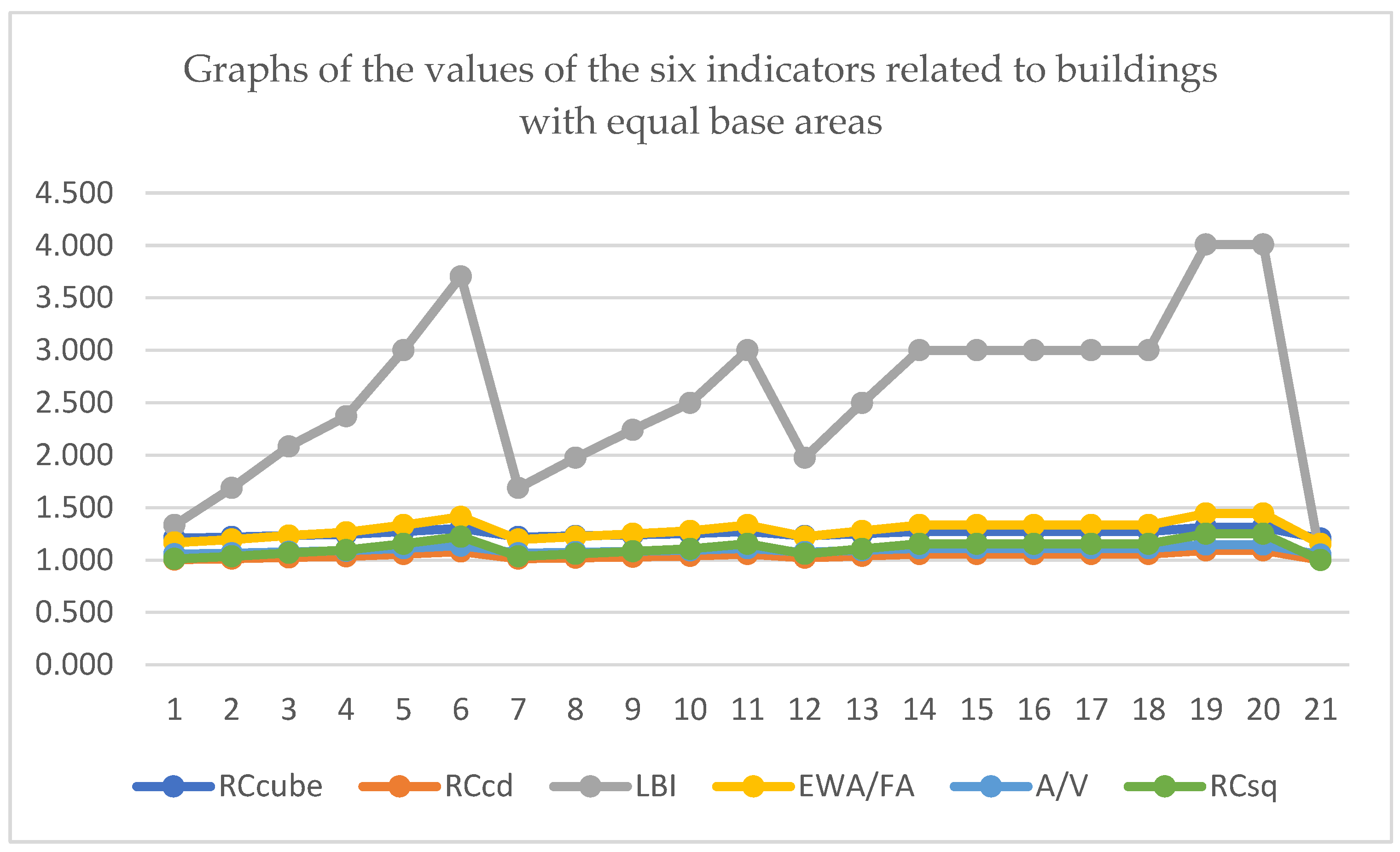The values of individual parameters and indicators are presented in Table 1. The last line is particularly interesting, where you can read the percentage deviation of the building’s external wall area from the optimal (smallest) area. According to the results of [27,28], these deviations translate into the embodied and functional energy of the buildings in question. The highest energy “losses” in relation to the ideal shape, i.e., the lowest geometric efficiency, are observed in buildings B6, B19, B20—22.2%, 25.1%, 25.1%, respectively. Buildings B5, B11, B14–B18 (all 15.4%) also have low geometric efficiency. The compactness assessment scale proposed in [20]: highly non-compact, non-compact, somewhat non-compact, neutral, somewhat compact, compact, and highly compact are expressed here with specific numbers (in percentage points). Geometric illustrations of building plans along with percentage deviations from the ideal shape can be found in Figure A1. We also note the mutual consistency of all indices except the $LBI$ index (Figure 1). This is not surprising, since in [28] linear dependencies between the indicators ${RC}_{cd}$, $EWA/FA$, $A/V$ were proven, assuming that ${\mathrm{A}}_{\mathrm{f}}$ and $\mathrm{h}$ are constant. However, the relationship between ${RC}_{cd}$ and ${RC}_{sq}$ is also linear as it is expressed by the formula below.

$${RC}_{cd}={\displaystyle \frac{\frac{1}{2}\sqrt{{\mathrm{A}}_{\mathrm{f}}}+{RC}_{sq}\mathrm{h}}{\frac{1}{2}\sqrt{{\mathrm{A}}_{\mathrm{f}}}+h}}.$$

(7)

With constants ${\mathrm{A}}_{\mathrm{f}}$ and $\mathrm{h}$, this is of course a linear relationship. An interesting relationship between the indicators can be observed in Figure 1. The numerical correlations between these indicators are equal to one. In particular, cor(RC_cd, RC_cube) = 1, cor(RC_cd, LBI) = 0.999256, cor(RC_sq, LBI) = 0.999256, cor(RC_cd, A/V) = 1, cor(RC_cd, A/V) = 1, cor(RC_cd, RC_sq) = 1. Only in the second and third cases does the correlation coefficient slightly differ from 1, but on the other hand, an algebraic linear relationship between the RC_cd and LBI indices, and thus between RC_sq and LBI, cannot be established. We will not obtain such a relationship in relation to real house designs for the reasons given earlier, at the beginning of this paragraph. However, the awareness that this relationship holds for theoretically adopted outlines is enough for the designer to use the ${RC}_{sq}$ indicator.

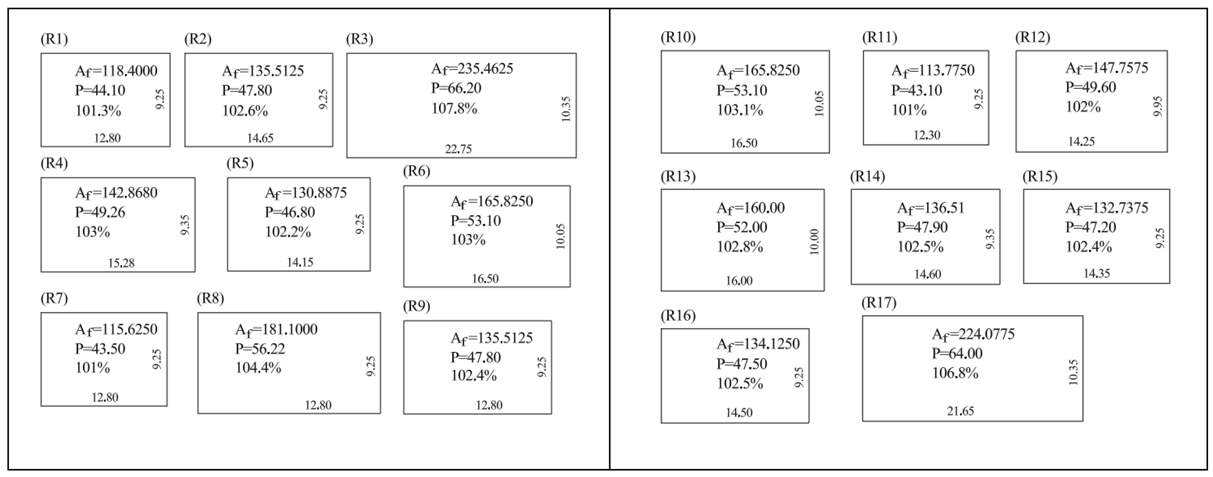
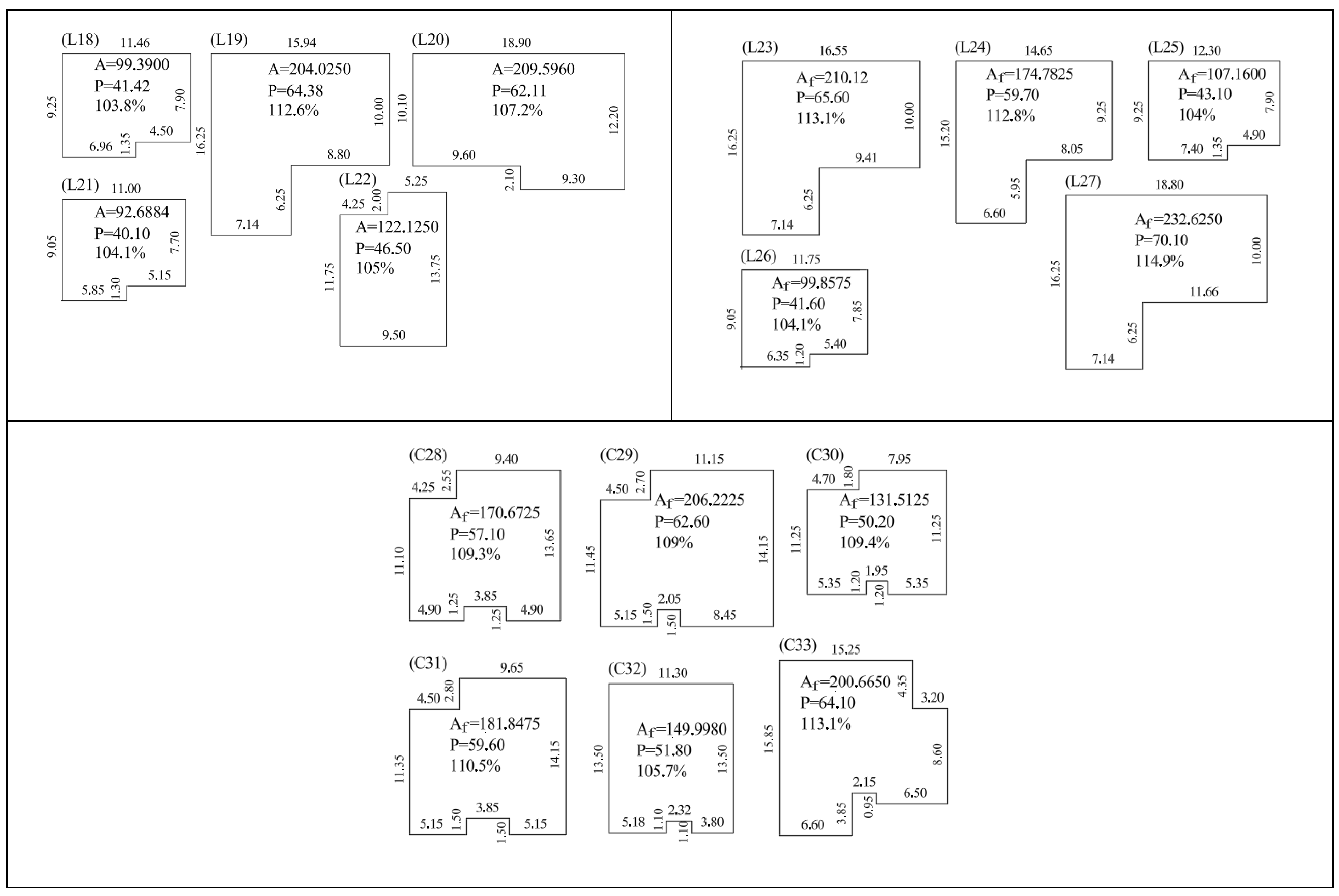
2.2. A Collection of Buildings Designed by the Design Studio

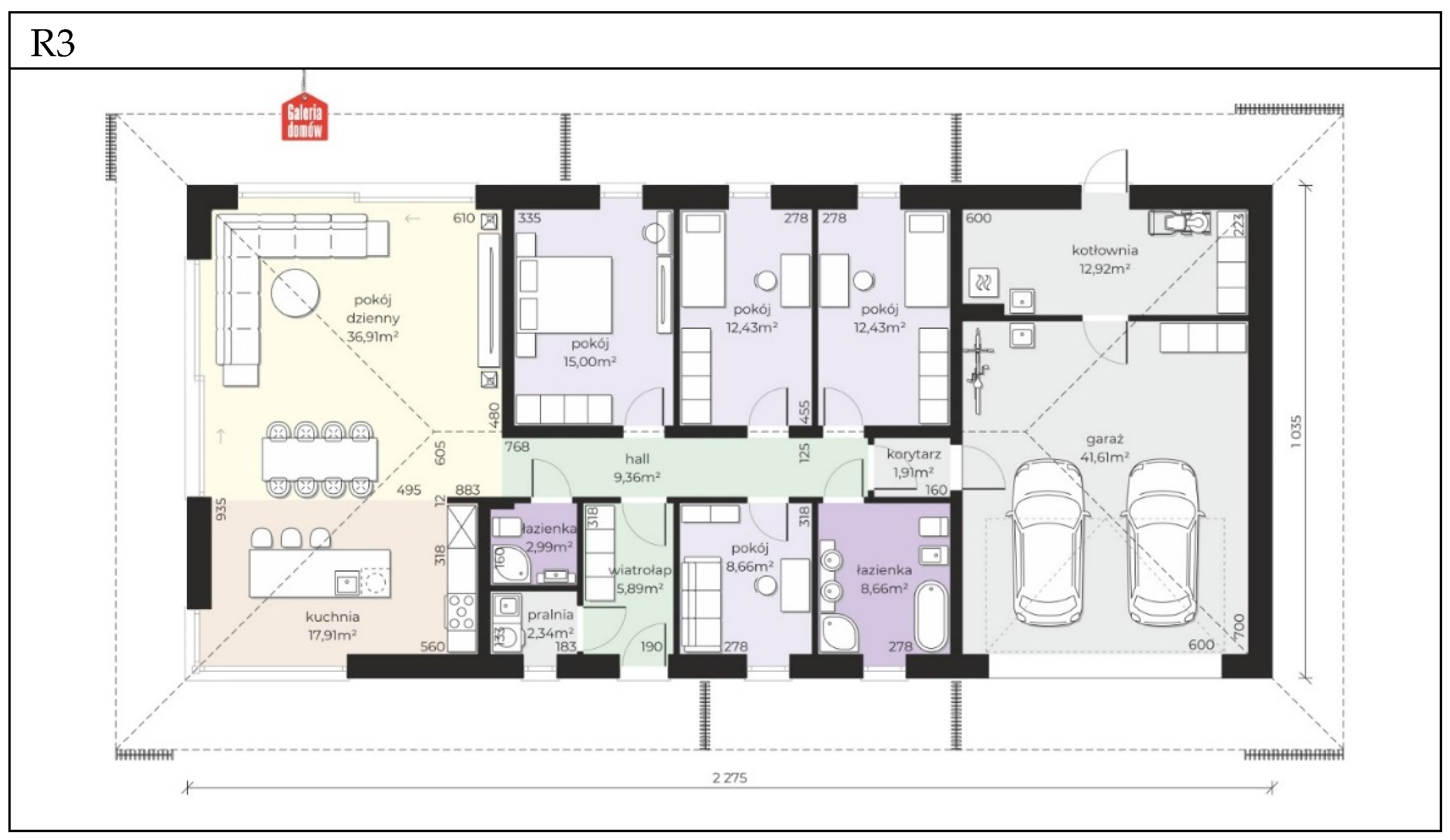
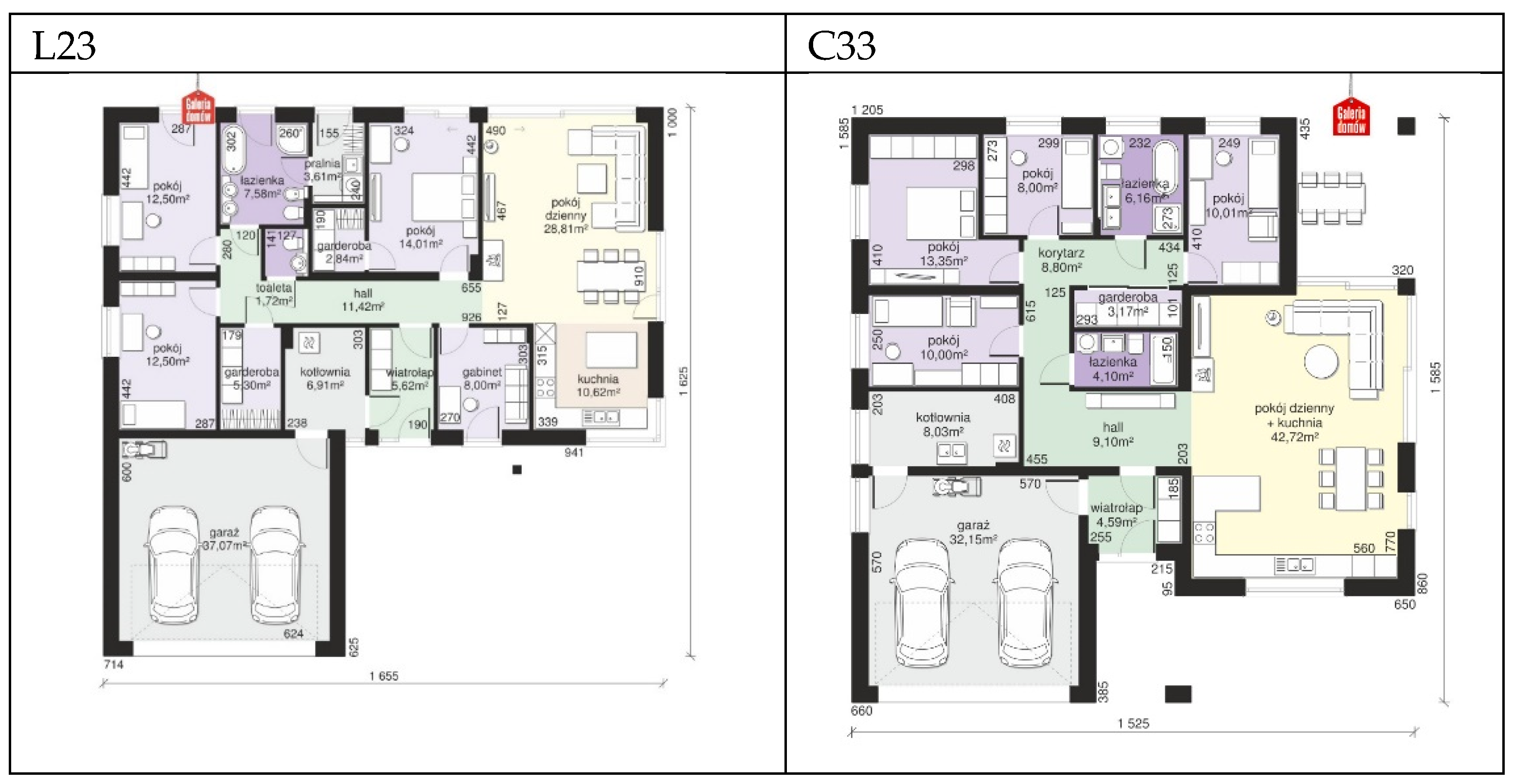
In this section we assess the geometric efficiency of single-family house plans designed by the Polish design office [31]. Due to the shape of the building outline, we divided the set of 33 houses into three subsets: 17 houses with a rectangular base marked by R1–R17 (Figure 2 and Figure A2), 10 houses with a rectangular polygon base in the shape of the letter L marked by L18–L27 (Figure 3 and Figure A3) and 6 houses in the shape of a rectangular polygon resembling the letter C marked by C28–C33 (Figure 3 and Figure A3). Example house plans with descriptions in Polish are included in Figure 2 and Figure 3.

For all 33 buildings we prepare schematic outlines (Figure A2 and Figure A3) and calculate the indicator values, which are presented in Table 1,

Table 2. (a) Basic geometrical parameters of the buildings L1–L9. (b) Basic geometrical parameters of the buildings L10–L17.

(a)
Parameter	Unit	Building Number
		R1		R2		R3		R4		R5		R6		R7		R8		R9
Af	m2	118.4000		135.5125		235.4625		142.8680		130.8875		165.8250		115.6250		181.1000		135.5125
P	m	44.10		47.80		66.20		49.26		46.80		53.10		43.50		56.22		47.80
h	m	3.00		3.00		3.00		3.00		3.00		3.00		3.00		3.00		3.00
RCcube	-	1.226		1.259		1.407		1.271		1.250		1.303		1.221		1.328		1.259
RCcd	-	1.005		1.009		1.022		1.010		1.007		1.010		1.004		1.014		1.009
LBI	-	1.384		1.584		2.198		1.634		1.530		1.642		1.351		1.811		1.584
EWA/FA	-	1.117		1.058		0.843		1.034		1.073		0.961		1.129		0.931		1.058
A/V	m−1	1.039		1.019		0.947		1.011		1.024		0.987		1.043		0.977		1.019
RCsq	-	1.013		1.026		1.078		1.030		1.023		1.031		1.011		1.044		1.026
Csq	%	101.3		102.6		107.8		103.0		102.3		103.1		101.1		104.4		102.6
(b)
Parameter	Unit	Building Number
		R10		R11		R12		R13			R14			R15		R16		R17
Af	m2	165.8250		113.7750		147.7575		160.0000			136.5100			132.7375		134.1250		224.0775
P	m	53.10		43.10		49.60		52.00			47.90			47.20		47.50		64.00
h	m	3.00		3.00		3.00		3.00			3.00			3.00		3.00		3.00
RCcube	-	1.303		1.218		1.274		1.294			1.259			1.253		1.256		1.390
RCcd	-	1.010		1.004		1.007		1.010			1.010			1.008		1.009		1.020
LBI	-	1.642		1.330		1.492		1.600			1.561			1.551		1.568		2.092
EWA/FA	-	0.961		1.136		1.007		0.975			1.053			1.067		1.062		0.857
A/V	m−1	0.987		1.045		1.002		0.992			1.018			1.022		1.021		0.952
RCsq	-	1.031		1.010		1.020		1.028			1.025			1.024		1.025		1.069
RCsq	%	103.1		101.0		102.0		102.8			102.5			102.4		102.5		106.9

,

Table 3. Basic geometrical parameters of the buildings L18–L27.

Parameter	Unit	Building Number
		L18	L19	L20	L21	L22	L23	L24	L25	L26	L27
Af	m2	99.3900	204.0250	209.5960	92.6884	122.1250	210.1200	174.7825	107.1600	99.8575	232.6250
P	m	41.42	64.38	62.11	40.10	46.50	65.60	59.70	43.10	41.60	70.10
h	m	3.00	3.00	3.00	3.00	3.00	3.00	3.00	3.00	3.00	3.00
RCcube	-	1.206	1.390	1.375	1.196	1.249	1.399	1.355	1.220	1.208	1.431
RCcd	-	1.015	1.038	1.021	1.016	1.018	1.038	1.040	1.015	1.015	1.042
LBI	-	1.741	2.710	2.132	1.773	1.900	2.757	2.732	1.768	1.766	2.941
EWA/FA	-	1.250	0.947	0.889	1.298	1.142	0.937	1.025	1.207	1.250	0.904
A/V	m−1	1.083	0.982	0.963	1.0993	1.047	0.979	1.008	1.069	1.083	0.970
RCsq	-	1.039	1.127	1.073	1.041	1.052	1.131	1.129	1.041	1.041	1.149
RCsq	%	103.8	112.7	107.3	104.1	105.2	113.1	112.9	104.1	104.1	114.9

and

Table 4. Basic geometrical parameters of the buildings C28–C33.

Parameter	Unit	Building Number
		C28	C29	C30	C31	C32	C33
Af	m2	170.6725	206.2225	131.5125	181.8475	149.9980	200.6650
P	m	57.10	62.60	50.20	59.60	51.80	64.10
h	m	3.00	3.00	3.00	3.00	3.00	3.00
RCcube	-	1.335	1.380	1.282	1.354	1.293	1.388
RCcd	-	1.029	1.026	1.032	1.032	1.019	1.039
LBI	-	2.350	2.320	2.368	2.480	1.963	2.756
EWA/FA	-	1.004	0.911	1.145	0.983	1.036	0.958
A/V	m−1	1.001	0.970	1.048	0.994	1.012	0.986
RCsq	-	1.093	1.090	1.094	1.105	1.057	1.131
RCsq	%	109.3	109.0	109.4	110.5	105.7	113.1

. As we said, we will be mainly interested in the ${RC}_{cd}$ indicator and the one expressed in percentage points. The last two lines indicate the deviation of the external surface areas of the building partitions from the optimum value (1.00 in the penultimate line/100% in the last line of all Table 1, Table 2, Table 3 and Table 4). These values provide a clear assessment of the geometric efficiency of the building. The values determined in this way translate into the amount of embodied energy related to the construction of the building (the amount of energy needed to produce materials and build the house in its raw state) [27].

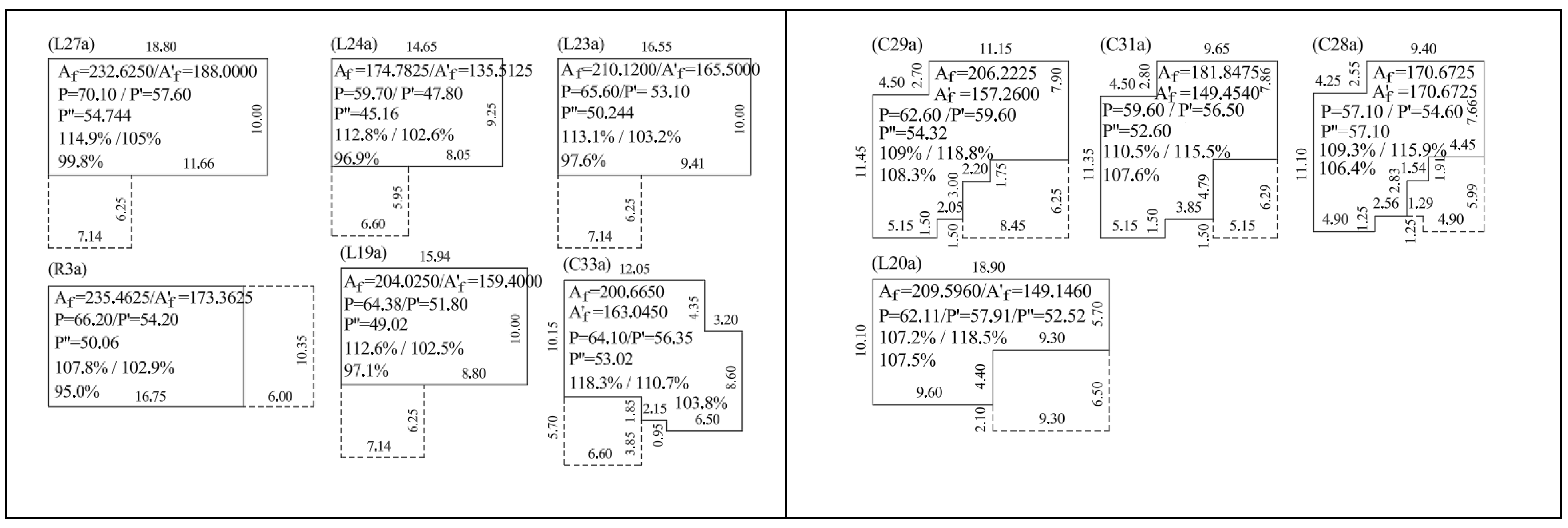
Among the 33 buildings, we have 10 houses with garages: R3, L19, L20, L23, L24, L27, C28, C29, C31, C33 (Figure A2 and Figure A3). In the energy analysis, in addition to the building outline, the outline of the heated part of the building should be considered (Figure A4). So we have two circuits P, P’ (Figure A4).

$$\mathrm{P}={\sum }_{i=1}^n{p}_i,$$

(8)

$${\mathrm{P}}^{\prime }={\sum }_{i=1}^m{p^{\prime }}_i,$$

(9)

where ${p^{\prime }}_k=p_k$, for some $k=1,2,\dots$,$m_1$ (after appropriate numbering and ordering of indices, of course $m_1<m$). The results of the calculation of the indicators for the heated part for ten houses with garages are presented in

Table 5. Basic geometrical parameters and compactness indicators of the buildings with garages in terms of the heated part (building designations were supplemented with the postfix a).

Parameter	Unit	Building Number
		L27a	L24a	L23a	R3a	L19a	C33a	C29a	C31a	L20a	L28a
A′f	m2	188.0000	135.5125	165.5000	173.3625	159.4000	162.0550	157.2600	149.4540	149.1460	138.5303
P′	m	57.60	47.80	53.10	54.20	51.80	56.35	59.60	56.50	57.91	54.60
h	m	3.00	3.00	3.00	3.00	3.00	3.00	3.00	3.00	3.00	3.00
RCcube	-	1.340	1.259	1.303	1.313	1.292	1.329	1.357	1.333	1.345	1.319
RCcd	-	1.015	1.009	1.010	1.009	1.008	1.034	1.061	1.051	1.061	1.054
LBI	-	1.880	1.584	1.655	1.618	1.572	2.498	3.348	3.007	3.320	3.052
EWA/FA	-	0.919	1.058	0.963	0.938	0.975	1.043	1.137	1.134	1.165	1.182
A/V	m−1	0.973	1.019	0.988	0.979	0.992	1.014	1.046	1.045	1.055	1.061
RC′sq	-	1.050	1.027	1.032	1.029	1.026	1.107	1.188	1.155	1.185	1.160
RC′sq	%	105.0	102.7	103.2	102.9	102.6	110.7	118.8	115.5	118.5	116.0

.

When calculating heat loss by transfer from a heated space to an unheated space, we use the temperature reduction factor $b_u$ $({0<b}_u\le 1)$ [32]. The value of coefficient $b_u$ depends on climatic conditions, type of adjacent room, partition structure (wall), etc., but is always less than 1 and thus improves the energy efficiency of the building. Then we can consider the so-called calculation perimeter P’’ taking into account the partitions bordering the unheated part, i.e., (after referring to the base polygon) the sides of the polygon that satisfy the condition ${p^{″}}_k={p^{\prime }}_k$ for $k=1,2,\dots ,l<m$ (after appropriate numbering and ordering of indices). The formula for the computational circuit, after appropriate numbering and ordering of the indices, then has the form

$${\mathrm{P}}^{″}={\sum }_{i=1}^{m_1}{p}_i+b_u{\sum }_{i=1}^{m_2}{p^{″}}_i,$$

(10)

where $m=m_1+m_2$.

The part of the geometric perimeter (marked in (10) in blue) bordering the buffer walls of the building (unheated room, e.g., garage) is numerically reduced, although geometrically it remains unchanged. Therefore, it may happen that the indicator (12) has a value less than 1 (in percentage points, a value less than 100%). We can then say that the building has a geometric efficiency better than a geometrically ideal building (see

Table 6. Parameters and compactness indicators of buildings with garages, taking into account the calculation perimeters in terms of the heated part (building designations were supplemented with the postfix ab).

Parameter	Unit	Building Number
		L27ab	L24ab	L23ab	R3ab	L19ab	C33ab	C29ab	C31ab	L20ab	L28ab
A′f	m2	188.0000	135.5125	165.5000	173.3625	159.4000	162.0550	115.6250	181.1000	135.5125	138.5303
P′	m	54.744	45.16	50.244	50.06	49.024	53.02	54.32	52.62	52.52	50.11
RC′sq	-	0.998	0.969	0.976	0.950	0.971	1.038	1.083	1.076	1.075	1.064
RC′sq	%	99.8	96.9	97.6	95.0	97.1	103.8	108.3	107.6	107.5	106.4

).

We will use the circuits in the characterization of energy consumption in the following way: the P perimeter is useful for describing the embedded energy, and the P′ and P″ circuits are convenient for calculating the functional energy. Using the formula

$${RC}_{sq}={\displaystyle \frac{{\mathrm{P}}^{\prime }}{4\sqrt{{{\mathrm{A}}^{\prime }}_{\mathrm{f}}}}},$$

(11)

we determine the values of the compactness indicators, which we place in Table 5.

If the unheated space has at least two external walls with optional external doors (e.g., garage, hall), the temperature reduction coefficient $b_u$ is equal to $b_u=$ 0.6 [32]. Therefore, when calculating heat losses for part of the perimeter we use this coefficient.

For 10 houses with garages, we will use the temperature reduction factor $b_u=$ 0.6 when calculating the compactness indicator. We will determine the computational perimeters $P^{″}$ from the data (Figure A4) using Formula (10) as follows.

• L27ab: ${\mathrm{P}}^{″}=18.80+2·10.00+11.66+0.6·7.14=54.744$,
• L24ab: ${\mathrm{P}}^{″}=14.65+2·9.25+8.05+0.6·6.66=45.16$,
• L23ab: ${\mathrm{P}}^{″}=16.55+2·10.00+9.41+0.6·7.14=50.244$,
• R3ab: ${\mathrm{P}}^{″}=2·16.75+10.35+0.6·10.35=50.06$,
• L19ab: ${\mathrm{P}}^{″}=15.94+2·10.00+8.80+0.6·7.14=49.024$,
• C33ab: ${\mathrm{P}}^{\mathrm{″}}=15.85+12.05+4.35+3.20+8.60+6.50+0.95+2.15+0.6·\left(1.85+6.60\right)=53.02$,
• C29ab:${\mathrm{P}}^{″}=2.05+1.50+5.15+11.45+4.50+2.70+11.15+7.90+0.6·\left(6.25+1.75+2.20+3.00\right)=54.32$,
• C31ab: ${\mathrm{P}}^{\mathrm{″}}=3.85+1.50+5.15+11.35+4.50+2.80+9.65+7.86+0.6·\left(5.15+4.79\right)=52.62$,
• L20ab: ${\mathrm{P}}^{\mathrm{″}}=9.60+10.10+18.90+5.70+0.6·\left(9.30+4.40\right)=52.52$.
• L28ab: ${\mathrm{P}}^{″}=7.66+9.40+2.55+4.25+11.10+4.90+1.25+2.56+0.6·\left(2.83+1.54+1.91+4.45\right)=50.11$.

Next, based on the formula

$${R{C}^{″}}_{sq}={\displaystyle \frac{{\mathrm{P}}^{″}}{4\sqrt{{{\mathrm{A}}^{\prime }}_{\mathrm{f}}}}},$$

(12)

we calculate the geometric efficiency indices for all buildings with garages and provide them in Table 6.

Note that the applied analysis will give good results in the case of terraced houses. If, for example, in a terraced house, we assume the plan of each house in the form of a square, and the number of houses is equal to $n$, then two houses will have one wall, and $n-2$ houses will have two walls with temperature reduction. This will give a very favorable result, definitely better than the ideal shape (base as a square) of geometric (energy) efficiency compared to detached houses.

3. Results and Discussion

Research (calculations) show that using the simplest possible RC_sq (RC′_sq, RC″_sq) indicator, expressed by two easily measurable parameters, ${\mathrm{A}}_{\mathrm{f}}$ and $\mathrm{P}$, we are able to constructively describe the geometric efficiency of a building in terms of energy.

3.1. Analysis of Energy Indicators for Theoretically Designed Buildings

The idea of considering examples of single-family houses B1–B21 with the same floor area, constructed theoretically, confirms the results obtained in the papers [27,28]. This confirms the sense of characterizing the geometry of buildings with a fixed building area. It shows that using easy-to-obtain quantities by the designer is very convenient at the initial design stage. The linear relationship of the indicators ${RC}_{cd}$, $EWA/FA$, ${RC}_{sq}$, and $A/V$ proves that each indicator well describes the geometric efficiency of the building. However, only the compactness index ${RC}_{sq}$ gives, in percentage points, an easily interpretable measure of the deviation from the optimal shape. The optimal shape is a building on a square plan. The analyzed building cases show that if we assume architecturally permissible dimensions (inducing a possible home design), the deviations in the area of external walls from the optimal shape can even exceed 25%. However, theoretically we can assume a rectangle with dimensions ${\displaystyle \frac{108}{q}}$ and $q$, as the base of the building. For $q$ = 1000 we have a rectangle with irrational dimensions of $1000\times 0.11$ [m] and ${RC}_{sq}=48.117$. In percentage points this gives a value of 4811.7%. In order to determine the numerical scale, one may wonder how large a deviation is possible for the shape of a rectangle to make architectural sense? In terraced houses this value can be quite large.

3.2. Analysis of Energy Indicator for Selected Buildings from the Collection of the Design Office

The values of the indicators in Table 2, Table 3 and Table 4 translate into both embodied and functional energy. This applies to cases where the entire building surface is heated, i.e., houses without garages. With respect to buildings with garages, Table 5 illustrates the transitional, theoretical stage. The values of the compactness indicators represent a situation in which the analysis of the heated part does not take into account the rest of the building. Hence, the percentage deviation values are relatively large and reach up to 19% (Table 5). However, after taking into account the temperature reduction factor $b_u$, these values drop to 7–8% in extreme cases. However, in the remaining cases the deviations even reach negative values: −0.2% (99.8–100 = 0.2), −3.1%, −2.4%, −5%, −2.9%, 3.8%, 8.3%, 7.6%, 7.7%, and 6.4% (Table 6). It means that, paradoxically, the shape of the house is better than ideal, in terms of functional energy demand. This result, coming only from the initial geometric analysis taking into account the temperature reduction coefficient, is a big surprise. It shows how important and universal the geometric analysis of the building’s shape is from the point of view of energy demand.

In general, the analysis of the ${RC}_{sq}$ indicator in versions (4), (11), and (12) for 33 real house designs indicates small deviations from the ideal shape. The lowest are in the collection of rectangular buildings, the maximum reached about 7% (houses R3 and R17). The lowest are in the collection of rectangular buildings, the maximum reached about 7% (houses R3 and R17). The analysis of the heated part also shows very good and good values of the compactness indicators in the designs of the design office.

4. Conclusions

The geometric optimization of a building’s shape is a universal way to search for solutions in the field of buildings with a low energy demand. The percentage deviations in the area of the building’s external walls from the reference building with a square base reflect the essence of the building’s geometric compactness very well. Taking the ${RC}_{sq}$ indicator in percentage terms as a measure in assessing the geometric compactness of buildings is the best solution was previously unknown in the literature. The houses designed by the Galeria Domów design office, assessed with the ${RC}_{sq}$ indicator from a geometric point of view, meet the geometric requirements of energy-saving buildings well or very well. The observations regarding negative deviations from the optimal shape (especially building R3, Table 6) confirm the favorable compactness of terraced houses.