Abstract
This study presents a novel approach in the field of renewable energy, focusing on the power generation capabilities of floating offshore wind turbines (FOWTs). The study addresses the challenges of designing and assessing the power generation of FOWTs due to their multidisciplinary nature involving aerodynamics, hydrodynamics, structural dynamics, and control systems. A hybrid deep learning model combining Convolutional Neural Networks (CNNs) and Long Short-Term Memory (LSTM) networks is proposed to predict the performance of FOWTs accurately and more efficiently than traditional numerical models. This model addresses computational complexity and lengthy processing times of conventional models, offering adaptability, scalability, and efficient handling of nonlinear dynamics. The results for predicting the generator power of a spar-type floating offshore wind turbine (FOWT) in a multivariable parallel time-series dataset using the Convolutional Neural Network–Long Short-Term Memory (CNN-LSTM) model showed promising outcomes, offering valuable insights into the model’s performance and potential applications. Its ability to capture a comprehensive range of load case scenarios—from mild to severe—through the integration of multiple relevant features significantly enhances the model’s robustness and applicability in realistic offshore environments. The research demonstrates the potential of deep learning methods in advancing renewable energy technology, specifically in optimizing turbine efficiency, anticipating maintenance needs, and integrating wind power into energy grids.
1. Introduction
The over-reliance on fossil fuels has led to pressing global challenges, including climate change and environmental degradation, primarily driven by greenhouse gas emissions from human activities [1]. Renewable energy sources have emerged as critical alternatives, offering sustainable and cleaner options to mitigate these issues. Among them, wind energy plays a pivotal role, accounting for approximately of the global renewable energy expansion, as reported by the International Energy Agency (IEA) [2]. Offshore wind energy, particularly in deep-sea environments, holds great promise due to its higher and more consistent wind speeds. Floating offshore wind turbines (FOWTs) have become a focal point in harnessing these resources efficiently [3]. However, designing and optimizing FOWTs remains highly complex, requiring a multidisciplinary approach that spans aerodynamics, hydrodynamics, structural dynamics, and control engineering. Traditionally, assessing the performance of FOWTs has relied on high-fidelity numerical simulations. While these models—such as those using OpenFAST or similar tools—are powerful, they often entail intensive computational costs and are sensitive to assumptions, input quality, and environmental variations [4,5]. Their scalability and adaptability are limited, especially when evaluating a wide range of operating conditions or turbine configurations. In contrast, data-driven approaches, particularly machine learning (ML), have emerged as powerful alternatives. These models can learn complex, nonlinear mappings from historical data and generalize across new scenarios with reduced computational load once trained [6,7]. Advanced ML algorithms—such as artificial neural networks (ANNs), support vector machines (SVMs), support vector regression (SVR), and neuro-fuzzy models—have been successfully applied to various aspects of wind energy systems, including short- and long-term time-series forecasting [8,9,10,11,12]. More recently, deep learning neural networks (DLNNs) have shown substantial promise in handling the inherent nonlinearities and temporal dependencies of offshore wind systems. Models like convolutional neural networks (CNNs), recurrent neural networks (RNNs), gated recurrent units (GRUs), and long short-term memory (LSTM) networks have been widely used in maritime and energy domains due to their ability to process sequential data and capture hidden temporal patterns [13,14,15,16,17]. For example, LSTM networks have been utilized to forecast wind speed and wave height using offshore NOAA buoy data, achieving RMSEs of and , respectively—enabling better metocean forecasting and turbine maintenance planning [18]. Beyond meteorological forecasting, deep learning has also been applied to structural health monitoring and load prediction in wind turbines [19,20]. Choe et al. [21] employed GRU and LSTM models to detect structural damage in FOWT blades. Similarly, Li et al. [22] integrated physics-based constraints into a deep residual RNN (DR-RNN) to predict dynamic responses of bottom-fixed offshore wind turbines, achieving a balance between data efficiency and model accuracy. Chen et al. [23] used a five-layer feedforward neural network trained on mooring load data from a coupled simulation to predict line tension under various scenarios, while Khazaee et al. [24] and several other efforts have focused on combining numerical model outputs with deep learning. Wang et al. [25] used OpenFAST-generated data to train a multi-layer perceptron (MLP) model for predicting tower responses. Similarly, Ostovar et al. [26] used MLP to optimize steel structure design. Pandit et al. [27] used an RNN for sequential condition monitoring of onshore turbines based on SCADA datasets. Despite notable advancements, the use of deep learning—particularly hybrid deep learning models—for directly predicting power output from FOWTs remains limited. Existing research has largely concentrated on load forecasting, structural health monitoring, or analysis of metocean parameters, with relatively few models developed for direct energy production prediction [28]. This study seeks to enhance machine learning techniques for forecasting the power output of FOWTs. To this end, we propose a novel hybrid deep learning framework that combines OpenFAST numerical simulations with a CNN-LSTM architecture to accurately predict power generation. This hybrid approach leverages the physical accuracy of OpenFAST and the data-driven adaptability of deep learning, offering improved prediction accuracy, reduced computational requirements, and practical relevance for real-time deployment in offshore wind operations.
2. Methodology
This section describes creating a CNN-LSTM model for estimating the power output of spar-type floating wind turbines. The deep learning model’s training, validating, and testing data are taken via the OpenFAST software. OpenFAST is a sophisticated open-source software developed by the National Renewable Energy Laboratory to simulate offshore wind turbines’ dynamic response and performance. It provides a comprehensive and accurate framework for modeling the entire wind turbine system, including aerodynamics, hydrodynamics, structural dynamics, and control system dynamics. The aim of this investigation is an NREL catenary anchored spar-type wind turbine. Configuration of the FOWT used in this study is shown in Figure 1 and its overall properties are listed in Table 1.
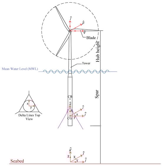
Figure 1.
Configuration of a spar-type FOWT, and the used coordinate systems [29].

Table 1.
Overall system properties of the 5 MW NREL wind turbine [1].
TurbSim [30], a cutting-edge numerical program designed for simulating wind fields in wind turbine performance studies, is used to construct eight turbulent wind fields with a mean horizontal wind velocity at the hup height varying from 10 to 24 m s−1. This wind speed range encompasses a broad range of operating conditions for floating offshore wind turbines (FOWTs), from mild to harsh environments. The upper limit of 24 m s−1 corresponds to the cut-out wind speed, at which the turbine’s control system engages to prevent excessive rotor speed, thereby protecting structural integrity and ensuring safe performance. The lower limit of 10 m s−1 represents the typical cut-in speed commonly adopted in similar studies [31]. As illustrated in Figure 2, these turbulent wind fields are subsequently employed as inputs for OpenFAST and the CNN-LSTM model. TurbSim can generate turbulent wind fields that accurately represent real-world circumstances, which is critical for accurate and dependable wind turbine simulations. TurbSim uses complex algorithms to simulate the stochastic character of wind, taking into account elements such as spatial coherence, turbulence strength, and the impact of atmospheric stability.
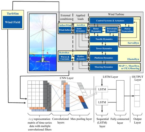
Figure 2.
Structure of the model.
This study also takes into account six sea conditions based on periodic sea states presented by [31], as shown in Table 2, as well as seven wind propagation directions with uniform distribution spanning from −30 to 30 degrees. The consideration of diverse sea state conditions, along with a broad range of wave propagation directions, significantly improves the model’s fidelity and representativeness of real-world scenarios. This method produced a thorough set of 336 simulations lasting 800 s, resulting in a robust analysis dataset using OpenFAST. The proposed hybrid CCN-LSTM model was developed in the Python programming environment.
Table 2.
Sea state data [31].
3. Convolutional Neural Network (CNN)
The Convolutional Neural Network (CNN) is a Deep Neural Network (DNN) model predominantly used in processing data with grid-like topology, like images [32]. CNNs are also widely used in financial market analysis, predicting stock price movements, and trend analysis, as demonstrated in various economic studies [33]. This versatility in handling complex visual and auditory data underlines its adaptability across different domains. The fundamental architecture of CNN draws inspiration from biological processes [34], particularly connectivity patterns in the animal visual cortex. This resemblance to biological neural networks has made CNN popular in areas such as image and video recognition, recommendation systems, image classification, medical image analysis [35], and natural language processing. Moreover, CNN’s efficiency in handling time-series data makes it a powerful tool for processing and analyzing such data. The capability to handle multichannel input data makes CNN highly suitable for managing diverse time-series data with multiple inputs and outputs. This multichannel processing capability enables CNN to capture a wide range of features from the input data, enhancing its predictive accuracy. Despite its widespread use, there is still a gap in research regarding CNN’s effectiveness in modeling and forecasting movements in multiple time-series data values within deep learning frameworks. This gap presents an opportunity for further exploration and innovation in the field. CNN can significantly reduce the number of parameters by its local receptive fields and shared weights. This reduction in parameters not only speeds up the learning process but also minimizes the risk of overfitting, making CNNs more robust and reliable. A CNN comprises three layers, including a convolutional layer, a pooling layer, and a fully connected layer. Each convolutional layer has multiple kernels performing convolution operations, extracting vital data features, and increasing feature dimensions. A pooling layer replaces the network’s output at specific locations by deriving a summary statistic of the nearby outputs to reduce the spatial size of representation and ease the training process, aiming to reduce the feature count and streamline the learning process. This combination of convolution and pooling layers enables CNNs to process and learn from complex data structures efficiently.
3.1. Long Short-Term Memory (LSTM)
Long short-term memory is a widely used neural network model designed to address the vanishing gradient problem that the RNN model faces. LSTM is capable of capturing long-term dependencies in complex trends, which makes it suitable for time-series prediction. The architecture of an LSTM network comprises three parts, commonly known as gates, that carry out specific functions. These gates are called the forgot gate, input gate, and output gate, respectively. The first part determines whether the information from the preceding timestamp should be remembered or is irrelevant and should be ignored. As a result, in the second phase, the cell assimilates new information from the input it receives. Finally, in the third section, the cell updates the information from the current timestamp to the next timestamp. This LSTM cycle is regarded as a one-time step. An LSTM, like a simple RNN, contains a hidden state where is the previous timestamp’s hidden state, and is the current timestamp’s hidden state. Furthermore, LSTM includes a cell state, denoted as and for the previous and current time steps. The forget gate is obtained through computation using the following formula:
in which is the hidden state weight matrix, denotes the output value of the previous time step, is the current time stamp input, and is the bias value applied to the forget gate. A sigmoid function is then applied to it. As a result, will be a value between 0 and 1. Next, the previous time’s output value and the present time’s input value are both fed into the input gate, and the input gate can be calculated using the following formula:
where is the weight matrix of the input gate, and is the bias value of the gate input candidate. The new information to be transferred to the cell state is determined by the function of the hidden state at the previous time step t − 1 and the input x at time step t, with the activation function being tanh. Owing to the tanh function, the new information’s value range lies between −1 and 1. Condition of the candidate cell at the input gate can be obtained as follows:
where represents the weight of the gate input candidate, while denotes the bias value associated with the gate input candidate. However, cannot be added directly to the cell state. The subsequent step in the LSTM model involves modifying cell values or model parameters at this point, which is executed as follows:
where is the cell state at the current time step. During processing at time t, the output value and the input value serve as inputs for the output gate. The output from this gate is then computed using the following formula:
similarly, is the weight for the gate output, and is the bias value at the output gate. Finally, the output gate generates the LSTM’s final output value, which is the result of a calculation using the following formula:
where tanh is the activation function. CNN and LSTM models can be used in time-series prediction, and each has its advantages and limitations. Combining these enables the model to capture secret trends in the data and avoid overfitting the training data.
3.2. Multivariate CNN-LSTM Model
Real-world data usually incorporates multiple variables, and the generated power of an FOWT is no exception. The value for this generated power depends on other features’ historical values, which makes this problem a multi-variable time-series analysis. Denoting these features by , the predicted value for at time t can be shown as follows:
in a similar way, prediction for the next component may be based on all previous values in the system. Then, a more general form of equation 7 can be considered for the forecast of the k-th variable as follows:
In a multivariate time-series, numerous variables change over time. Each of these variables is influenced not just by its own preceding values but also by the values of other variables. is a multiple time-series comprised of a set time-series where k is the series index, and t is the time point. Similar to univariate time-series analysis, the primary objective of multiple time-series analysis is to identify suitable functions , where q represents the number of functions formulated, which can effectively predict future values of a variable while maintaining desirable properties.
3.3. Feature Engineering
The present study employs OpenFAST software to obtain a set of 336 outputs for dynamic response analysis and power prediction of a spar-type FOTW. Considering the Nyquist criterion, dynamic system characteristics, numerical stability criteria, and guidelines from OpenFAST documentation and iterative testing, the time step for all simulations is set to 0.0125 s, which is small enough to accurately capture the dynamic characteristics of the system and avoid numerical instability. Each output file comprises 141 columns that reflect various features, and because each simulation lasts 800 s, each output file contains a total of 64,002 rows. To avoid introducing noises to the model prediction and capture dependencies and trends in generated power, the sampling frequency of data decreased to 1 s. Next, all output files are combined to create a comprehensive dataset for the deep learning model. The correlations between generated power and other features were examined in order to identify features whose previous values may be relevant in predicting generated power future values. From the correlation analysis, nine features that are highly correlated with power generation were chosen (Figure 3).
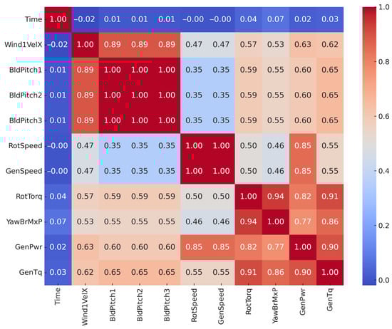
Figure 3.
Heatmap of correlation between parameters.
Table 3 shows a sample of the dataset used in this study and Figure 4 indicates the wind velocity in the x direction and generated power time-series for one of the load cases. is the wind velocity in the x direction; , , and are the pitch angles of blades 1, 2, and 3, respectively. is the turbine rotor speed, refers to the generator speed, represents the torque exerted on the rotor of the wind turbine, is the non-rotating tower-top/yaw bearing roll moment, is electrical generator power, and is electrical generator torque. Moreover, a unique ID indicates each load case to be able to trace back the performance of the model for individual load cases. Only a subset of five routinely recorded Supervisory Control and Data Acquisition (SCADA) channels, , 1–3, , and , are retained for modeling and is included only in an optional ablation. These measurements are available on any modern turbine without additional hardware and, taken alone, cannot be algebraically combined to recreate generator power at the same instant, because torque channels and other drivetrain variables that would close that loop are purposely excluded. Restricting the feature set in this way keeps the model practical for real-time deployment and removes the risk of target leakage while still capturing the causal chain from wind inflow to structural response.
Table 3.
Sample of selected features from OpenFAST output data.
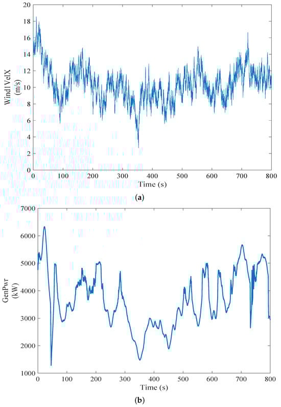
Figure 4.
(a) Wind velocity (m s−1) in x direction and (b) generated power (kW) for load case w3s1d1.
The proposed model also incorporates a technique for creating lagged features to capture temporal dependencies and trends within the dataset. Lagged features are essentially previous time steps of a time-series used as separate input features. This method works especially well for time-series forecasting, which is based on the idea that historical data will have a big impact on future data. By introducing a lag of n time steps, each relevant feature in the dataset is transformed into a series of its past values, which provides the model with a richer context for making predictions. Using a lag of 10 in this study, each observation in the dataset included not only the current value of a feature but also its values from the previous 10 time points. This method effectively enabled the model to learn from the sequential nature of the data, recognizing patterns and trends that unfold over time. This approach allows the neural network, especially models like LSTMs, to better understand and learn from the chronological sequence of the data, which is crucial in scenarios where temporal dynamics are important. To eliminate data leakage, the 336 OpenFAST simulations were concatenated and then partitioned by simulation in chronological order into training, validation, and test sets; every time-series segment in the validation and test splits therefore occurs strictly later in time than all samples seen during model fitting, and all normalization scalers are derived from the training split only. During inference, the model advances with a rolling-window scheme: the most-recent ten-step window of the nine selected input features is fed to the trained CNN-LSTM to yield a one-second-ahead estimate of generator power. Once the window reaches the test portion, no ground-truth test data are revealed to the model; it progresses auto-regressively, sliding the window forward each second and filling any missing inputs with its own previous predictions.
The proposed hybrid deep learning architecture combining CNN and LSTM networks uses the Sequential API from Keras-TensorFlow, which is a high-level neural network library used for time-series data processing. In this architecture, local features are extracted by CNNs, where LSTM layers capture long-term dependencies to predict generated power. The first layer is a 1D convolutional (Conv1D) with 120 filters and a kernel size of three. This layer uses the ReLU activation function and is designed to process the input sequence data. The choice of 120 filters is a design parameter representing the number of feature maps generated, and the kernel size of three indicates the width of the convolutional window. After each convolutional layer, a max-pooling layer (MaxPooling1D) with a pool size of two is also applied. This pooling layer reduces the dimensionality of the data, which reduces computational load and controls overfitting by providing an abstracted form of representation. The model used in this study incorporates LSTM layers. The first LSTM layer has 50 units and returns sequences, which means it outputs the entire hidden state sequence. The training process is then stabilized and accelerated using a batch normalization layer. The next layer is the second LSTM layer with 50 units without returning sequences. It simply returns the output of the latest time step, thus capturing the long-term dependencies of the data. Following this LSTM layer is another batch normalization layer. The final layer of the model is a dense layer (Dense) with a single unit. The single unit indicates that the model generates a single continuous value or probability score. The Adam optimizer is used to compile the model, which is a common choice for deep learning applications due to its efficiency in dealing with sparse gradients and flexible learning rate capabilities. The loss function in this study is set to mean squared error, which is a common choice for regression situations [36]. Figure 5 indicates the basic structure of the proposed multivariate CNN-LSTM model for multiple time-series prediction with 14 features and ten time steps for the prediction process.
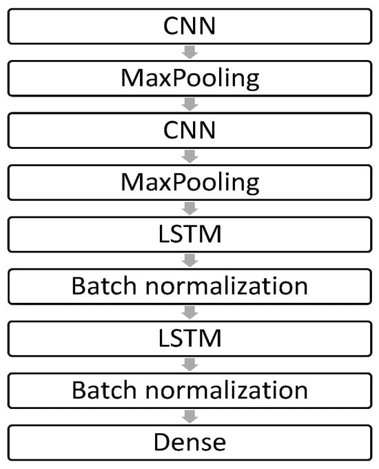
Figure 5.
Architecture of the CNN-LSTM model.
3.4. Model Evaluation
For evaluation of the predictive model, the Mean Squared Error () is employed as a key metric to quantify the accuracy of the model’s predictions against the actual observed values. The MSE is calculated using the following formula:
where represents the actual values, represents the predicted values by the model, and n is the number of observations. This metric is particularly effective in capturing the average squared difference between the estimated values and the actual value, thus providing a comprehensive measure of the model’s prediction error [37]. A lower value is indicative of a model with higher accuracy predictions. The was used to rigorously assess the model’s performance, ensuring that the insights derived are both reliable and indicative of the model’s capability to generalize across diverse data scenarios. Due to its robustness and sensitivity to big errors, the mean square error ensures that the model evaluation stays in line with the reality of practical application in real-world scenarios, particularly in situations when the cost of large errors is particularly significant.
4. Results and Discussion
This study proposes a Convolutional Neural Network-Long Short-Term Memory (CNN-LSTM) model developed to predict the generator power of a spar-type FOWT in a multivariable parallel time-series dataset. Results from training and subsequent evaluation of test data are promising and offer insight into the model’s performance and potential applications. The results obtained from the model architecture used in this study were then compared to a simple two-layer LSTM model with the same number of neurons as the LSTM layers implemented to show the proposed model’s capabilities and improvements in predicting turbine-generated power. The model achieved a loss of 0.0331 during training and a significantly lower validation loss of 0.016, suggesting that the model is learning generalizable patterns and performing exceptionally well on unseen data. This could be attributed to the effective architecture of the CNN-LSTM model, which benefits from the strengths of both CNNs in feature extraction from time-series and LSTMs in understanding long-term dependencies in such complex datasets.
The on test data is approximately 0.016. This low value of test data prediction MSE indicates a high level of accuracy in the model’s predictions. Since is sensitive to data scale and outliers, it shows that the model’s predictions closely match the actual values of generator power. The test data prediction for simple two-layer LSTM is 0.021, which does not show a significant improvement for this study’s suggested hybrid model architecture. Still, further comparisons revealed that the LSTM model’s tendency to overfit certain load cases in such complicated multi-variable parallel time-series could falsely cause reports for low overall . In contrast, it shows poor results for some other load cases. Figure 6 compares the for normalized generated power values predicted using the LSTM model and the proposed CNN-LSTM model in this study for three load cases. As can be seen, LSTM cannot capture dependencies in the load case despite having a relatively small overall for predicted data.
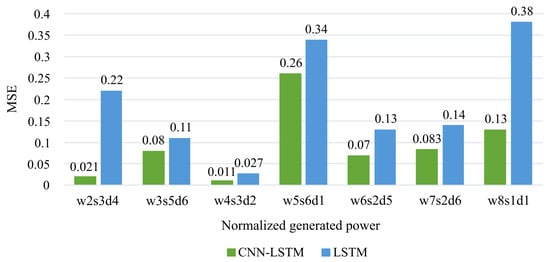
Figure 6.
MSE comparison between CNN-LSTM, and LSTM models on normalized target values.
Figure 7 demonstrates the model’s strong capability in capturing complex patterns and interactions among the features. The load case naming convention uses the number after ‘w’ to indicate the wind field, the number after ‘s’ to specify the sea state, and the number after ‘d’ to denote the wind direction. For example, ‘’ corresponds to a load case involving the eighth wind field, a sea state of one, and a wind direction (‘’) at −30 degrees relative to the central axis of the turbine hub. Figure 7 shows the time-series of predicted and actual data for three load cases shown in Figure 6 considering the 200 s feature’s data. The proposed model captures complex trends and dependencies to the features exceptionally well. On the contrary, the two-layer LSTM model shows poor results in capturing spatial features and trends (Figure 8). A comparison between Figure 7 and Figure 8 highlights the superior predictive performance and trend-capturing capability of the proposed CNN-LSTM model relative to the conventional LSTM model.
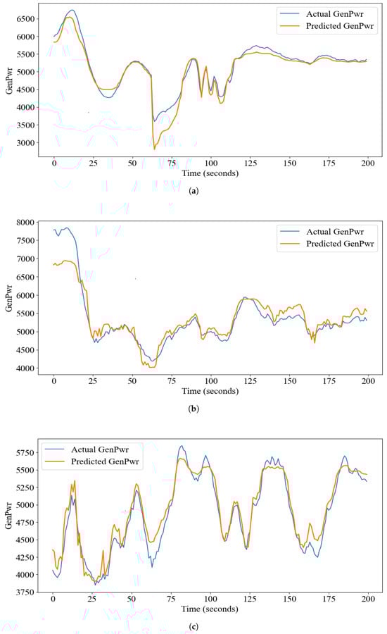
Figure 7.
Actual and generated power (kW) using CNN-LSTM model for load case (a) w2s3d4, (b) w6s2d5 and (c) w8s1d1.
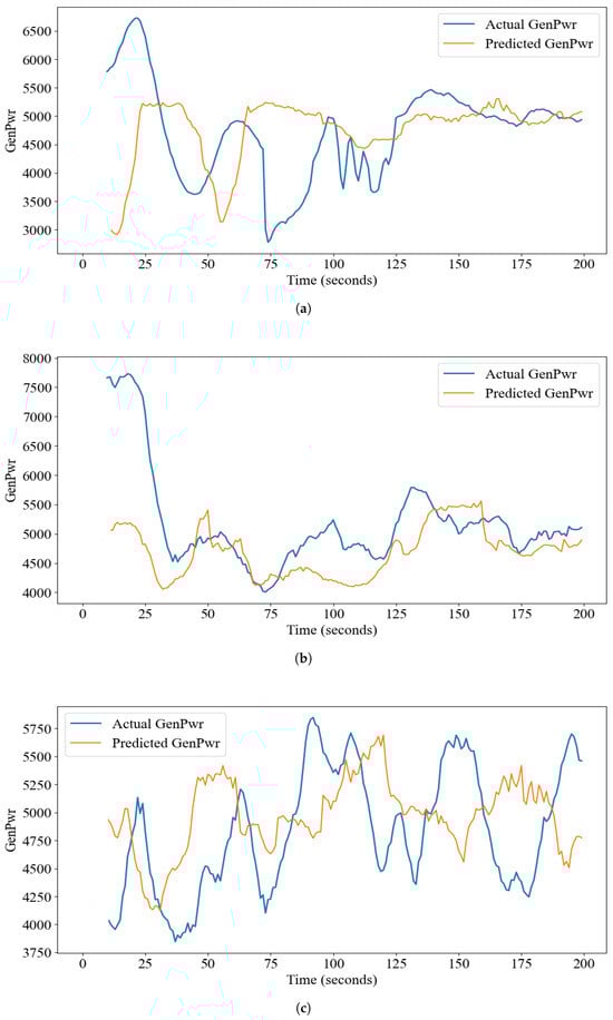
Figure 8.
Actual and generated power (kW) using LSTM model for load case (a) w2s3d4, (b) w6s2d5 and (c) w8s1d1.
From a computational time perspective, although this factor is highly dependent on the specific hardware configuration used, machine learning models typically require substantial time for training. However, once training is complete, the prediction phase is computationally efficient and executes rapidly.
In statistical measures of the model’s error (residual) analysis, several critical aspects of the model’s predictive behavior were discerned. The model’s minor tendency to underestimate the target variable is continuously hinted at by the mean of the errors, which stands at −0.029. Despite its mildness, this trend is notable for its relative consistency, and the small mean error magnitude indicates that there is no major bias toward either overestimation or underestimation. This inference is further supported by the median of the errors, which stands at −0.030. The mean and median both have negative values and are closely aligned, which highlights a consistent pattern of small underestimation across the model’s predictions.
Furthermore, the 0.027 value recorded for the standard deviation of the errors indicates that the majority of the errors are tightly clustered around the mean error; deviations from the expected values being neither exceedingly large nor widespread shows consistent level of accuracy in the model’s predictions. But an interesting feature shows up when you look at the skewness of the errors, which are estimated to be 0.948. This number denotes a moderate right skew in the error distribution, pointing to a tendency toward overestimation being more common than the overall underestimate trend, though not as widespread.
The model’s negative mean and median, on the one hand, indicate a general bias towards minor under-prediction. Conversely, the positive skewness indicates that the bigger mistakes in the model are biased toward over-prediction. Therefore, the model is generally accurate and consistent, exhibiting very minor underestimations on average and a tendency for more substantial overestimation, albeit less frequently.
Figure 9 shows the residual and Figure 10 gives the distribution of the residual for the model in this study.
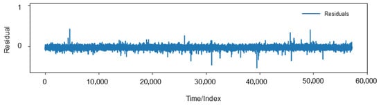
Figure 9.
Residual of the model.
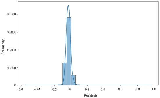
Figure 10.
Distribution of residuals.
The successful application of the CNN-LSTM model for predicting FOWT’s generated power has several implications. It highlights the efficacy of hybrid models that integrate convolutional and recurrent neural networks in dealing with complex time-series data with several features and spatial dependencies. Capturing spatial (by CNN) and temporal (via LSTM) interdependence is critical for successful time-series forecasting. Moreover, the high accuracy of the proposed model opens avenues for practical applications in the field to which the data pertains. Accurately predicting FOWT’s generator power can improve operating efficiency, enable preventative maintenance, and optimize resource allocation.
5. Summary and Conclusions
The present study introduces a novel hybrid deep learning framework for accurately predicting the power output of FOWTs. The proposed CNN-LSTM model is designed to address the inherent complexities and nonlinear behaviors associated with the multidisciplinary nature of FOWTs, encompassing aerodynamics, hydrodynamics, structural dynamics, and control systems. The research outcomes demonstrate the model’s superior predictive accuracy and precision, validated using Mean Squared Error (MSE) as the performance metric. The model shows significant promise in enhancing turbine performance optimization and supporting predictive maintenance strategies by significantly reducing the computational burden and processing time compared to conventional high-fidelity numerical models. One of the principal strengths of the proposed model is its capacity to capture a broad spectrum of load case scenarios and sea state conditions—ranging from mild to severe—through the integration of multiple relevant features, thereby enhancing its applicability and robustness in realistic offshore environments. With its high level of precision, the model enables improved turbine efficiency, supports predictive maintenance, and facilitates optimal resource allocation. Beyond its technical achievements, this work highlights the transformative role of Artificial Intelligence (AI) and machine learning in reshaping energy systems, offering a robust foundation for future innovations in the pursuit of sustainable and efficient energy solutions. From a practical standpoint, this approach supports more efficient power management, proactive maintenance planning, and improved integration of offshore wind energy into power grids. Looking ahead, future work may extend this methodology by incorporating real-world SCADA datasets, exploring transfer learning techniques for model portability, and integrating physics-informed neural networks (PINNs) to further enhance interpretability and reliability. Ultimately, this research offers a valuable step toward scalable, intelligent, and real-time forecasting solutions in the evolving field of offshore renewable energy.
Author Contributions
Conceptualization, M.B. (Mohammad Barooni); methodology, P.S. and M.B. (Masoumeh Bahrami); investigation, M.B. (Mohammad Barooni) and D.V.S.; resources, D.V.S.; data curation, M.B. (Mohammad Barooni), P.S. and M.B. (Masoumeh Bahrami); writing—original draft preparation, M.B. (Mohammad Barooni); writing—review and editing, D.V.S.; visualization, M.B. (Mohammad Barooni) and D.V.S.; supervision, D.V.S. All authors have read and agreed to the published version of the manuscript.
Funding
This research received no external funding.
Data Availability Statement
The original contributions presented in this study are included in the article. Further inquiries can be directed to the first and corresponding author(s).
Conflicts of Interest
The authors declare no conflict of interest.
References
- Barooni, M.; Nezhad, S.K.; Ali, N.A.; Ashuri, T.; Sogut, D.V. Numerical study of ice-induced loads and dynamic response analysis for floating offshore wind turbines. Mar. Struct. 2022, 86, 103300. [Google Scholar] [CrossRef]
- Barooni, M.; Ashuri, T.; Velioglu Sogut, D.; Wood, S.; Ghaderpour Taleghani, S. Floating Offshore Wind Turbines: Current Status and Future Prospects. Energies 2022, 16, 2. [Google Scholar] [CrossRef]
- Ashuri, T.; Zaaijer, M.B. Review of design concepts, methods and considerations of offshore wind turbines. In Proceedings of the European Offshore Wind Conference and Exhibition, Berlin, Germany, 4–6 December 2007; Volume 1. [Google Scholar]
- Xu, Y.; Liu, P.; Penesis, I.; He, G.; Heidarian, A.; Ghassemi, H. Energy generation efficiency and strength coupled design and optimization of wind turbine rotor blades. J. Energy Eng. 2019, 145, 04019004. [Google Scholar] [CrossRef]
- Junejo, A.R.; Gilal, N.U.; Doh, J. Physics-informed optimization of robust control system to enhance power efficiency of renewable energy: Application to wind turbine. Energy 2023, 263, 125667. [Google Scholar] [CrossRef]
- Del Ser, J.; Casillas-Perez, D.; Cornejo-Bueno, L.; Prieto-Godino, L.; Sanz-Justo, J.; Casanova-Mateo, C.; Salcedo-Sanz, S. Randomization-based machine learning in renewable energy prediction problems: Critical literature review, new results and perspectives. Appl. Soft Comput. 2022, 118, 108526. [Google Scholar] [CrossRef]
- Gogas, P.; Papadimitriou, T. Machine Learning in Renewable Energy. Energies 2023, 16, 2260. [Google Scholar] [CrossRef]
- Kim, S.; Matsumi, Y.; Pan, S.; Mase, H. A real-time forecast model using artificial neural network for after-runner storm surges on the Tottori coast, Japan. Ocean Eng. 2016, 122, 44–53. [Google Scholar] [CrossRef]
- Dineva, A.; Várkonyi-Kóczy, A.R.; Tar, J.K. Fuzzy expert system for automatic wavelet shrinkage procedure selection for noise suppression. In Proceedings of the IEEE 18th International Conference on Intelligent Engineering Systems INES 2014, Tihany, Hungary, 3–5 July 2014; pp. 163–168. [Google Scholar]
- Suykens, J.A.; Vandewalle, J. Recurrent least squares support vector machines. IEEE Trans. Circuits Syst. I Fundam. Theory Appl. 2000, 47, 1109–1114. [Google Scholar] [CrossRef]
- Gizaw, M.S.; Gan, T.Y. Regional flood frequency analysis using support vector regression under historical and future climate. J. Hydrol. 2016, 538, 387–398. [Google Scholar] [CrossRef]
- Taherei Ghazvinei, P.; Hassanpour Darvishi, H.; Mosavi, A.; Yusof, K.b.W.; Alizamir, M.; Shamshirband, S.; Chau, K.w. Sugarcane growth prediction based on meteorological parameters using extreme learning machine and artificial neural network. Eng. Appl. Comput. Fluid Mech. 2018, 12, 738–749. [Google Scholar] [CrossRef]
- Brownlee, J. Deep Learning for Time Series Forecasting: Predict the Future with MLPs, CNNs and LSTMs in Python; Machine Learning Mastery: Melbourne, Australia, 2018. [Google Scholar]
- Hinton, G.; Deng, L.; Yu, D.; Dahl, G.E.; Mohamed, A.r.; Jaitly, N.; Senior, A.; Vanhoucke, V.; Nguyen, P.; Sainath, T.N.; et al. Deep neural networks for acoustic modeling in speech recognition: The shared views of four research groups. IEEE Signal Process. Mag. 2012, 29, 82–97. [Google Scholar] [CrossRef]
- El Bourakadi, D.; Ramadan, H.; Yahyaouy, A.; Boumhidi, J. A novel solar power prediction model based on stacked BiLSTM deep learning and improved extreme learning machine. Int. J. Inf. Technol. 2023, 15, 587–594. [Google Scholar] [CrossRef]
- Xiong, J.; Peng, T.; Tao, Z.; Zhang, C.; Song, S.; Nazir, M.S. A dual-scale deep learning model based on ELM-BiLSTM and improved reptile search algorithm for wind power prediction. Energy 2023, 266, 126419. [Google Scholar] [CrossRef]
- Lim, S.C.; Huh, J.H.; Hong, S.H.; Park, C.Y.; Kim, J.C. Solar Power Forecasting using CNN-LSTM hybrid model. Energies 2022, 15, 8233. [Google Scholar] [CrossRef]
- Barooni, M.; Ghaderpour Taleghani, S.; Bahrami, M.; Sedigh, P.; Velioglu Sogut, D. Machine Learning-Based Forecasting of metocean data for offshore engineering applications. Atmosphere 2024, 15, 640. [Google Scholar] [CrossRef]
- Li, H.; Huang, C.G.; Soares, C.G. A real-time inspection and opportunistic maintenance strategies for floating offshore wind turbines. Ocean Eng. 2022, 256, 111433. [Google Scholar] [CrossRef]
- Abbas, N.; Zalkind, D.; Pao, L.; Wright, A. A reference open-source controller for fixed and floating offshore wind turbines. Wind Energy Sci. Discuss. 2021, 2021, 1–33. [Google Scholar] [CrossRef]
- Choe, D.E.; Kim, H.C.; Kim, M.H. Sequence-based modeling of deep learning with LSTM and GRU networks for structural damage detection of floating offshore wind turbine blades. Renew. Energy 2021, 174, 218–235. [Google Scholar] [CrossRef]
- Li, X.; Zhang, W. Physics-informed deep learning model in wind turbine response prediction. Renew. Energy 2022, 185, 932–944. [Google Scholar] [CrossRef]
- Chen, H.; Liu, H.; Chu, X.; Liu, Q.; Xue, D. Anomaly detection and critical SCADA parameters identification for wind turbines based on LSTM-AE neural network. Renew. Energy 2021, 172, 829–840. [Google Scholar] [CrossRef]
- Khazaee, M.; Derian, P.; Mouraud, A. A comprehensive study on Structural Health Monitoring (SHM) of wind turbine blades by instrumenting tower using machine learning methods. Renew. Energy 2022, 199, 1568–1579. [Google Scholar] [CrossRef]
- Wang, Z.; Qiao, D.; Tang, G.; Wang, B.; Yan, J.; Ou, J. An identification method of floating wind turbine tower responses using deep learning technology in the monitoring system. Ocean Eng. 2022, 261, 112105. [Google Scholar] [CrossRef]
- Ostovar, A.; Davari, D.D.; Dzikuć, M. Determinants of design with Multilayer Perceptron Neural Networks: A comparison with logistic regression. Sustainability 2025, 17, 2611. [Google Scholar] [CrossRef]
- Pandit, R.; Astolfi, D.; Hong, J.; Infield, D.; Santos, M. SCADA data for wind turbine data-driven condition/performance monitoring: A review on state-of-art, challenges and future trends. Wind Eng. 2023, 47, 422–441. [Google Scholar] [CrossRef]
- Sun, Y.; Zhou, Q.; Sun, L.; Sun, L.; Kang, J.; Li, H. CNN–LSTM–AM: A power prediction model for offshore wind turbines. Ocean Eng. 2024, 301, 117598. [Google Scholar] [CrossRef]
- Barooni, M.; Ali, N.A.; Ashuri, T. An open-source comprehensive numerical model for dynamic response and loads analysis of floating offshore wind turbines. Energy 2018, 154, 442–454. [Google Scholar] [CrossRef]
- Jonkman, B.J. TurbSim User’s Guide; Technical Report; National Renewable Energy Lab. (NREL): Golden, CO, USA, 2006.
- Jonkman, J. Definition of the Floating System for Phase IV of OC3 (No. NREL/TP-500-47535); National Renewable Energy Lab. (NREL): Golden, CO, USA, 2010.
- O’Shea, K.; Nash, R. An introduction to Convolutional Neural Networks. arXiv 2015, arXiv:1511.08458. [Google Scholar]
- Lu, W.; Li, J.; Li, Y.; Sun, A.; Wang, J. A CNN-LSTM-based model to forecast stock prices. Complexity 2020, 2020, 6622927. [Google Scholar] [CrossRef]
- Deldadehasl, M.; Jafari, M.; Sayeh, M.R. Dynamic classification using the adaptive competitive algorithm for Breast Cancer Detection. J. Data Anal. Inf. Process. 2025, 13, 101–115. [Google Scholar] [CrossRef]
- Mahdavi, Z. Introduce improved CNN model for accurate classification of autism spectrum disorder using 3D MRI brain scans. In Proceedings of the MOL2NET’22, International Conference on Molecular, Biomedicine, Computational & Network Science and Engineering, 8th ed.; MDPI: Basel, Switzerland, 2022. [Google Scholar]
- Breiman, L.; Olshen, R.A. Points of Significance: Classification and regression trees. Nat. Methods 2017, 14, 757–758. [Google Scholar]
- Hodson, T.O.; Over, T.M.; Foks, S.S. Mean squared error, deconstructed. J. Adv. Model. Earth Syst. 2021, 13, e2021MS002681. [Google Scholar] [CrossRef]
Disclaimer/Publisher’s Note: The statements, opinions and data contained in all publications are solely those of the individual author(s) and contributor(s) and not of MDPI and/or the editor(s). MDPI and/or the editor(s) disclaim responsibility for any injury to people or property resulting from any ideas, methods, instructions or products referred to in the content. |
© 2025 by the authors. Licensee MDPI, Basel, Switzerland. This article is an open access article distributed under the terms and conditions of the Creative Commons Attribution (CC BY) license (https://creativecommons.org/licenses/by/4.0/).