Predicting the Evolution of Capacity Degradation Histograms of Rechargeable Batteries Under Dynamic Loads via Latent Gaussian Processes

Abstract

Accurate prediction of lithium-ion battery capacity degradation under dynamic loads is crucial yet challenging due to limited data availability and high cell-to-cell variability. This study proposes a Latent Gaussian Process (GP) model to forecast the full distribution of capacity fade in the form of high-dimensional histograms, rather than relying on point estimates. The model integrates Principal Component Analysis with GP regression to learn temporal degradation patterns from partial early-cycle data of a target cell, using a fully degraded reference cell. Experiments on the NASA dataset with randomized dynamic load profiles demonstrate that Latent GP enables full-lifecycle capacity distribution prediction using only early-cycle observations. Compared with standard GP, long short-term memory (LSTM), and Monte Carlo Dropout LSTM baselines, it achieves superior accuracy in terms of Kullback–Leibler divergence and mean squared error. Sensitivity analyses further confirm the model’s robustness to input noise and hyperparameter settings, highlighting its potential for practical deployment in real-world battery health prognostics.

1. Introduction

1.1. Literature Review

Rechargeable batteries, particularly lithium-ion batteries, have gained widespread global application across important fields such as electric vehicles [1], energy storage stations [2], and portable devices [3]. However, even under regular operating conditions, repeated charge and discharge cycling inevitably induces degradation processes, primarily including solid electrolyte interphase (SEI) layer growth leading to irreversible lithium loss, and active material loss reducing lithium storage capacity [4,5,6]. These degradation mechanisms are strongly influenced by usage profiles, and their cumulative effects typically manifest as observable capacity fade that intensifies over cycling [7,8]. Thus, understanding and predicting battery capacity degradation is crucial for battery configuration and management, helping to prevent unexpected performance losses and safety hazards during usage.

Battery capacity degradation trajectory prediction has long been a core topic in battery research. Early studies focused on developing mathematical models that established relationships between cycle count and capacity degradation trends, using functions such as linear, polynomial, or exponential models to quantify future degradation [9,10,11]. Other approaches utilized recursive models, including autocorrelation models and autoregressive integrated moving average (ARIMA) models, to predict future capacity based on historical data [12,13,14]. While these foundational methods provided useful quantitative frameworks, they have been continually refined and improved upon over time, giving rise to more sophisticated models. Notably, some studies have integrated electrochemical modeling into capacity degradation prediction to enhance physical interpretability. Lyu et al. [15] identified key degradation-related physical parameters using an electrochemical model and extrapolated their evolution via exponential functions to forecast capacity fade. Ren et al. [16] developed a capacity degradation model by coupling a pseudo-two-dimensional electrochemical model, a three-dimensional thermal model, and an SEI formation model, enabling recursive prediction of future capacity loss. Although such semi-quantum models show promise in improving interpretability, their application in real-world scenarios remains limited due to data scarcity and computational complexity. Recent advancements in deep learning technologies have led to the development of even more advanced models, such as neural networks, which aim to bridge the gap between historical data and future predictions [17,18]. For instance, Huang et al. [19] utilized long short-term memory (LSTM) and convolutional neural networks (CNNs) to predict capacity trajectories by incorporating historical capacity, rest time, and internal resistance. Zhao et al. [20] applied multi-channel dependent neural networks to map incremental capacity and capacity differentials to critical future degradation points. Yang et al. [21] employed a CNN–Transformer–Kolmogorov–Arnold network to connect historical charging data with future capacity degradation. Similarly, Du et al. [22] bridged the relationship between historical charge/discharge cycles and future capacity degradation through CNNs. While these approaches have achieved success, they mostly rely on assumptions of constant load conditions, ignoring the dynamic load environments that batteries encounter in real-world applications [23]. As a result, their predictive outcomes may lack practical relevance, particularly when batteries operate under complex dynamic conditions.

In recent years, dynamic load-based battery capacity degradation prediction has emerged as a key research focus. Notably, the National Aeronautics and Space Administration (NASA) released a dataset detailing battery degradation under dynamic load conditions, revealing a nonlinear scatter in capacity degradation, which formed a capacity distribution rather than a single trajectory [24,25,26]. This starkly contrasts with the continuous degradation trends observed under constant load in earlier studies, prompting widespread academic interest in dynamic load effects on battery performance. Lu et al. [27] further analyzed battery capacity degradation under uncertain current excitation, revealing nonlinear oscillation patterns that emerge when current excitation changes unpredictably. They proposed a method for accurately predicting degradation based on future dynamic excitation plans. Subsequent research [28] confirmed that battery performance during charging and discharging varies based on load conditions, reinforcing the need to consider dynamic loads in capacity predictions.

While these studies incorporate future load plans to account for load capacity dependency, accurate prediction of such plans remains a prerequisite. Obtaining precise future load plans in practical applications is challenging, and the limited availability of degradation samples further complicates the predictive process [29,30]. Therefore, predicting future capacity histograms under dynamic loads without explicit knowledge of future load plans remains a critical issue to address.

To overcome these challenges, this paper presents a Latent Gaussian Process (LGP)-based method for predicting battery capacity histograms, particularly under dynamic load conditions. The contributions of this study are as follows:

(1) Dynamic load capacity prediction: This paper proposes a method for predicting battery capacity degradation histograms that reflect dynamic load conditions, offering a more accurate representation of degradation in real-world scenarios.

(2) Prediction of capacity degradation histograms: In contrast to traditional trajectory-based predictions, this work provides probability histograms of future degradation based on historical distribution patterns, delivering more comprehensive prediction results.

(3) Adaptability to small sample sizes: Compared to deep learning techniques, this approach excels in scenarios with limited data, effectively predicting capacity degradation even with sparse datasets, without the heavy reliance on large data volumes required by deep learning models.

1.2. Article Organization

The rest of the article is organized as follows. Section 2 presents the methodology, followed by Section 3, which discusses the experimental results and performance analysis. Finally, conclusions are drawn in Section 4.

2. Methodology

2.1. Framework of Methodology

The proposed framework aims to predict the future capacity degradation distribution of lithium-ion batteries under dynamic operating conditions. As illustrated in Figure 1, the proposed method consists of three main stages: histogram construction, latent space modeling, and probabilistic forecasting via Gaussian processes.

First, a sliding window is applied to the capacity degradation trajectory of the target battery, converting sequential capacity values into a series of histograms that describe the statistical distribution of capacity within each window. This histogram representation transforms the problem from single-point prediction into a distributional forecasting task, allowing the model to capture the inherent stochasticity of battery degradation.

Next, the high-dimensional histograms are projected into a lower-dimensional latent space using principal component analysis. This step extracts the dominant components that capture the major variations in degradation behavior, significantly reducing computational complexity and noise sensitivity.

Then, each principal component is modeled using a separate Gaussian Process. These GPs learn the temporal evolution of latent variables across different cycles, enabling robust extrapolation beyond the observed data.

Finally, the predicted latent components are reconstructed back into the histogram space, yielding forecasts of the full capacity degradation distribution over future cycles. This approach ensures that inter-bin correlations are preserved and uncertainty is naturally quantified via the GP’s posterior variance.

2.2. Battery Capacity Histogram Definition

The battery capacity histogram at the t-th cycle can be represented by a histogram over a sliding window:

$$\mathit{H}(t)=[h_1(t),h_2(t),\dots ,h_K(t)],t=1,2,\dots ,T$$

(1)

where H(t) is the battery capacity histogram at the t-th cycle, K is the total number of bins and h_k(t) is the frequency of capacity in the k-th bin, which is expressed as follows:

$$h_k(t)={\displaystyle \sum _{i=1}^{W}g(Q_i(t)\in B_k)}$$

(2)

where W is the length of the sliding window, Q_i(t) is the capacity value at the t-th cycle for the i-th measurement within the sliding window, g(·) is the indicator function, which is 1 if the condition inside the parentheses is true (i.e., if the capacity value Q_i(t) falls within bin B_k) and 0 otherwise, and B_k denotes the k-th bin of the predefined capacity histogram, covering a fixed range of capacity values, which can be described as follows:

$$B_k=[Q_{\min }+(k-1)\cdot \mathrm{\Delta }Q,Q_{\min }+k\cdot \mathrm{\Delta }Q)$$

(3)

where ΔQ is the capacity step size, which can be specified based on the chosen resolution, Q_min is the capacity failure threshold and k is the bin index, which ranges from 1 to K. The sum of the histogram bins at each cycle corresponds to the length of the sliding window, as it reflects the number of samples within the sliding window:

$${\displaystyle \sum _{k=1}^K{h}_k(t)}=W$$

(4)

2.3. Principal Component Analysis

Principal Component Analysis (PCA) [31] is used in this paper to reduce the dimensionality of the observed battery capacity histograms, H(t), and project them into a latent space where the most significant patterns of capacity degradation can be more effectively modeled. Each capacity degradation trajectory is initially represented as a high-dimensional distribution, where each cycle of degradation corresponds to a capacity histogram with multiple bins. However, to model the degradation process effectively, we first reduce the dimensionality of these histograms. This reduction is performed by PCA, which projects the high-dimensional data into a lower-dimensional latent space.

This approach is one of the key reasons why the method is referred to as a Latent Gaussian Process. Instead of directly applying the Gaussian process to the high-dimensional capacity histograms, we first apply PCA to H(t), reducing the data to K-dimensional latent variables. These reduced components are then used as inputs for Gaussian process regression, significantly simplifying the modeling process. This latent space transformation allows us to capture the key features of the degradation behavior while discarding less important details, providing a more efficient and accurate modeling approach.

To prepare the data for PCA, we first center and standardize the capacity histograms H(t) at each cycle. Centering ensures that each distribution has zero mean, and standardization ensures that each feature has unit variance, making the data suitable for PCA:

$${\mathit{H}}_{\mathrm{c}}(t)=\mathit{H}(t)-{\mu }_H$$

(5)

where μ_H represents the mean capacity distribution across all cycles.

Next, we calculate the covariance matrix C, which captures the relationships between the different bins of the capacity histograms:

$$\mathit{C}={\displaystyle \frac{1}{N-1}}{\mathit{H}}_{\mathrm{c}}{(t)}^{\mathrm{T}}{\mathit{H}}_{\mathrm{c}}(t)$$

(6)

where N is the number of cycles. This covariance matrix is essential for PCA to identify the correlations between capacity bins.

PCA involves solving the eigenvalue problem for the covariance matrix C. The eigenvectors v_k represent the principal components, and the eigenvalues λ_k correspond to the variance explained by each component:

$$\mathit{C}{\mathit{v}}_k={\mathit{v}}_k{\lambda }_k$$

(7)

These eigenvectors are ordered by the magnitude of their corresponding eigenvalues, and the principal components with the largest eigenvalues are selected for the latent space.

After identifying the principal components, we project the centered data H_c(t) onto the space spanned by these components:

$$\mathit{Z}(t)={\mathit{H}}_{\mathrm{c}}(t)\mathit{V}$$

(8)

where Z(t) is the data projected into the lower-dimensional latent space and V is the matrix of eigenvectors (principal components).

The number of principal components d is selected based on the explained variance. We choose d such that the cumulative explained variance exceeds a threshold, ensuring that the most significant patterns in the data are retained. In our case, d = 5 components are chosen to represent the most critical variations in capacity degradation behavior, while reducing dimensionality:

$$E={\displaystyle \frac{{\displaystyle \sum _{k=1}^d{\lambda }_k}}{{\displaystyle \sum _{k=1}^K{\lambda }_k}}}$$

(9)

where E is the explained variance ratio. This step ensures that the latent space captures the key degradation features and provides a compact representation of the original high-dimensional data.

2.4. Gaussian Processes

In this study, we perform Gaussian process regression [32] on each of the d principal components derived from the PCA process. Let Z(t) = [z₁(t), z₂(t), …, z_d(t)]^T denote the vector of latent variables (principal components) at cycle t, which corresponds to the battery capacity histogram H(t) projected into the lower-dimensional latent space using PCA. Each component z_k(t) represents the value of the k-th principal component at cycle t.

For each k∈{1, 2, …, d}, a separate GPR model is used to predict the trajectory of the corresponding latent variable z_k(t) over cycle. The general form of the model for each principal component z_k(t) is given by

$$z_k(t)=f_k(t)+{\epsilon }_k(t)$$

(10)

where f_k(t) represents the underlying smooth function that governs the evolution of the k-th principal component over time and ε_k(t) is the Gaussian noise term, capturing the uncertainty or errors in the observations of the k-th component.

Each f_k(t) can be modeled as a Gaussian Process:

$$z_k(t)\sim GP({\mu }_k(t),k_k(t,t\prime ))$$

(11)

where μ_k(t) is the mean function, which is assumed to be zero, and k_k(t, t’) is the covariance function (kernel), which defines the correlation between cycles for the k-th component. A typical choice for the kernel is the squared exponential kernel, which ensures smoothness and captures correlations between nearby cycles.

The GPR models are trained separately for each of the d principal components, with the observed data used to infer the latent function f_k(t) and the noise term ε_k(t). After training, these models can predict future values of the z_k(t), allowing us to forecast the battery capacity degradation in the latent space. These predicted latent components Z_pred(t) are then combined with the inverse PCA transformation to reconstruct the future capacity histograms Y_pred(t):

$${\mathit{Y}}_{\mathrm{pred}}(t)={\mathit{Z}}_{\mathrm{pred}}(t){\mathit{V}}^{\mathrm{T}}+\mu$$

(12)

To obtain normalized histogram values, we apply the Softmax function [33] and scale the predictions by the length of the sliding window to ensure the total sum of the distribution is W:

$${\mathit{Y}}_{\mathrm{pred}}^{\mathrm{norm}}(t)=W\cdot \mathrm{Softmax}({\mathit{Y}}_{\mathrm{pred}}(t))$$

(13)

where ${\mathit{Y}}_{\mathrm{pred}}^{\mathrm{norm}}$(t) is the final output of the proposed method.

2.5. Evaluation Metrics

The performance of the prediction model is evaluated using two key metrics: Kullback–Leibler (KL) divergence and mean squared error (MSE) [34].

The Kullback–Leibler divergence KL measures the difference between the true and predicted distributions, which can be computed as follows:

$$KL={\displaystyle \sum _{k=1}^K{y}_{\mathrm{true},k}^{\mathrm{norm}}\log (\frac{y_{\mathrm{true},k}}{y_{\mathrm{pred},k}^{\mathrm{norm}}})}$$

(14)

The mean squared error MSE evaluates the overall error between the true and predicted distributions, which can be defined as follows:

$$MSE={\displaystyle \frac{1}{K}}{\displaystyle \sum _{k=1}^K{(y_{\mathrm{true},k}-y_{\mathrm{pred},k}^{\mathrm{norm}})}^2}$$

(15)

3. Results

3.1. Datasets

To evaluate the performance of the proposed latent Gaussian process-based model in predicting capacity histogram evolution under dynamic loads, we employed the Randomized Battery Usage 7: Low-Temperature Left-Skewed Random Walk dataset provided by NASA’s Prognostics Center of Excellence. This dataset comprises four commercial 18,650 lithium-ion cells (identified as RW13, RW14, RW15, and RW16) that were continuously cycled under a randomized loading protocol designed to emulate real-world current variability. In each cycle, the batteries were first charged to 4.2 V using a constant-current/constant-voltage (CC/CV) scheme and then discharged to 3.2 V following a random walk discharge pattern. During discharge, the current setpoint was updated every 60 s. The new current value was drawn from a customized left-skewed probability distribution favoring lower currents. The available setpoints ranged from 0.5 A to 5.0 A, with selection probabilities as follows: 0.5 A (7.2%), 1.0 A (14.8%), 1.5 A (19.3%), 2.0 A (21.6%), 2.5 A (14.6%), 3.0 A (10.0%), 3.5 A (6.5%), 4.0 A (4.0%), 4.5 A (1.5%), and 5.0 A (0.5%).

The discharge capacity degradation of four cells (i.e., RW13, RW14, RW15, and RW16) over time under dynamic current loads are shown in Figure 2. It is worth noting that the RW16 curve in Figure 2d presents a visible gap between mid-November and mid-December 2014, which reflects a discontinuity in the original dataset rather than any data preprocessing issue. The results highlight that despite identical testing protocols, the degradation behaviors of different cells under randomized dynamic loads exhibit significant variability. The dynamic loading conditions lead to capacity degradation patterns that are not confined to a single trajectory but instead manifest as dispersed scatter trends. Moreover, the degree of dispersion increases with cycling, emphasizing the stochastic nature of battery aging. This further validates the necessity of capturing the distribution of capacity degradation rather than relying solely on deterministic point estimates when predicting battery health under realistic operating conditions.

3.2. Predictive Performance

To evaluate the predictive performance of the proposed method under a practical small-sample setting, we consider a scenario where the complete degradation trajectory of battery RW13 is available, while only the first 100 cycles of RW14, RW15, and RW16 are observed. The objective is to predict the capacity degradation histograms of RW14–RW16 from the 100th cycle until end-of-life. The prediction results are illustrated in Figure 3.

As shown in Figure 3a,e,i, the actual degradation histograms of RW14–RW16 exhibit considerable variability despite identical test protocols. Nevertheless, leveraging the full degradation data from RW13 and the early-cycle data from each target battery, the proposed method accurately reconstructs the capacity degradation histograms, closely matching the measured histograms in Figure 3b,f,j.

To quantitatively assess prediction accuracy, we report the KL divergence and MSE between the predicted and actual histograms in Figure 3c,g,k and Figure 3d,h,l, respectively. The results show that the maximum KL divergence remains below 3, with the median value under 2, indicating strong distributional consistency. Meanwhile, the maximum MSE does not exceed 0.16, and the median remains below 0.03, confirming the high fidelity of the predicted degradation patterns.

These results demonstrate that the proposed approach can effectively infer future degradation histograms using limited early-cycle data, offering a promising solution for data-efficient battery lifetime prognosis under dynamic operational conditions.

3.3. Comparison with Conventional Baselines

To demonstrate the effectiveness of the proposed Latent GP method, we design three comparative baseline models. The first baseline uses a standard GP without dimensionality reduction, directly modeling the high-dimensional capacity degradation histograms. This model shares the same hyperparameters as the proposed Latent GP to ensure a fair comparison. The second baseline employs an LSTM network, a widely used deep learning approach for time-series forecasting. The LSTM network takes the sliding window of historical capacity histograms as input and iteratively predicts future distributions. The network consists of two LSTM layers (each with 30 hidden units), followed by a fully connected layer for dimensional mapping and ReLU activation to ensure non-negativity of the output. It was trained for 200 epochs using the ADAM optimizer with a learning rate of 0.02 and MSE as the loss function. The third baseline introduces a Monte Carlo Dropout LSTM model, which shares the same architecture and training setup as the standard (MC) LSTM but adds dropout layers with a rate of 0.3 before each LSTM and fully connected layer. During inference, dropout is retained to enable stochastic forward passes that approximate a Bayesian posterior distribution [35]. A total of 30 such passes are performed at each prediction step, and the final prediction is obtained by averaging the results. These comparisons were conducted under the same setup: RW13 served as the reference battery with complete capacity degradation data, and RW14 was the target battery. Predictions began at the 100th cycle. The results are shown in Figure 4.

Figure 4a–d illustrate that the Latent GP most closely reproduces the measured degradation histograms (cf. Figure 3a). In contrast, the LSTM and MC Dropout LSTM models fail to capture the degradation patterns over time. The MC Dropout variant provides slightly less noisy predictions than the deterministic LSTM but still lacks the ability to track capacity decline. The standard GP performs better than both LSTM-based models but remains less accurate than the Latent GP. Its scattered predictions may result from its inability to model the dominant components of degradation processes.

Figure 4e–h quantify performance using KL divergence and MSE. The LSTM model exhibits the highest KL divergence, often exceeding 20, indicating a significant mismatch with the true distribution. The MC Dropout LSTM reduces the KL divergence to below 9 and achieves a median MSE around 0.01, suggesting that Bayesian approximation improves generalization and robustness. The standard GP maintains KL divergence below 7 but reaches an MSE above 0.02. In contrast, the Latent GP achieves both KL divergence below 3 and MSE below 0.015. These gains are attributed to the use of PCA, which captures the intrinsic structure of histogram evolution and enhances long-term forecast stability.

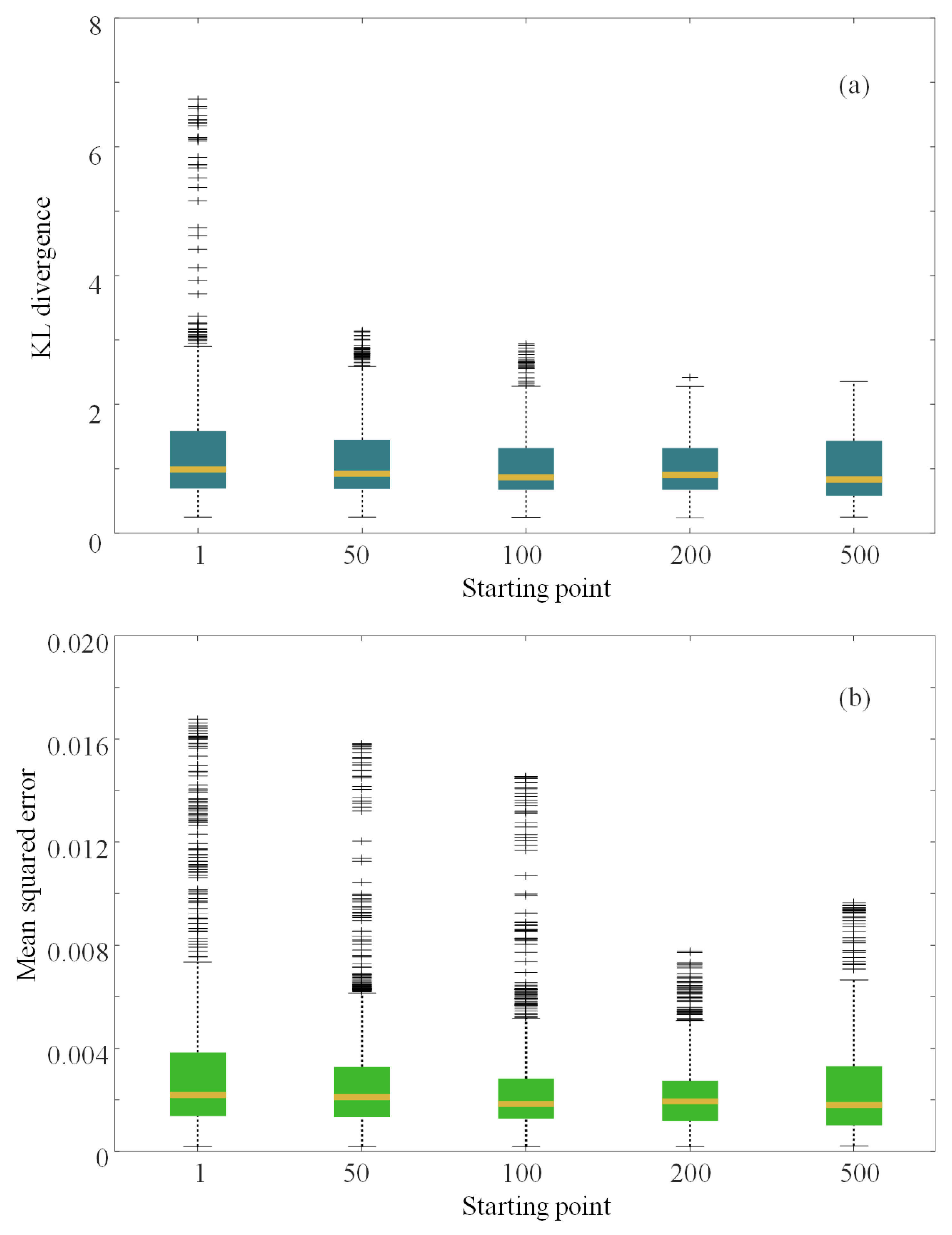
3.4. Performance with Different Starting Points

To explore the predictive performance under varying data availability, we conducted simulations assuming the complete capacity degradation data of the RW13 battery is known. The target battery in this analysis is RW14. We varied the starting point of prediction, altering the ratio between available historical data and the future degradation trajectory to be predicted. Specifically, the starting points were set at cycles 1, 50, 100, 200, and 500 to simulate different levels of prior information.

The boxplots for KL divergence (Figure 5a) and MSE (Figure 5b) are shown for each starting point. As the number of available cycles increases, both the KL divergence and MSE reduce, indicating that a higher proportion of historical data contributes to improved prediction accuracy. Specifically, when starting from cycle 1, the predictions exhibit higher divergence and error, which steadily decrease as more cycles are included for training. Starting from cycle 100 and beyond provides relatively stable prediction results, with the KL divergence and MSE values remaining low, indicating that predictions based on a larger portion of historical data are more accurate.

These results suggest that the predictive performance improves significantly when more historical data are incorporated, emphasizing the importance of early-cycle data in refining capacity degradation forecasts.

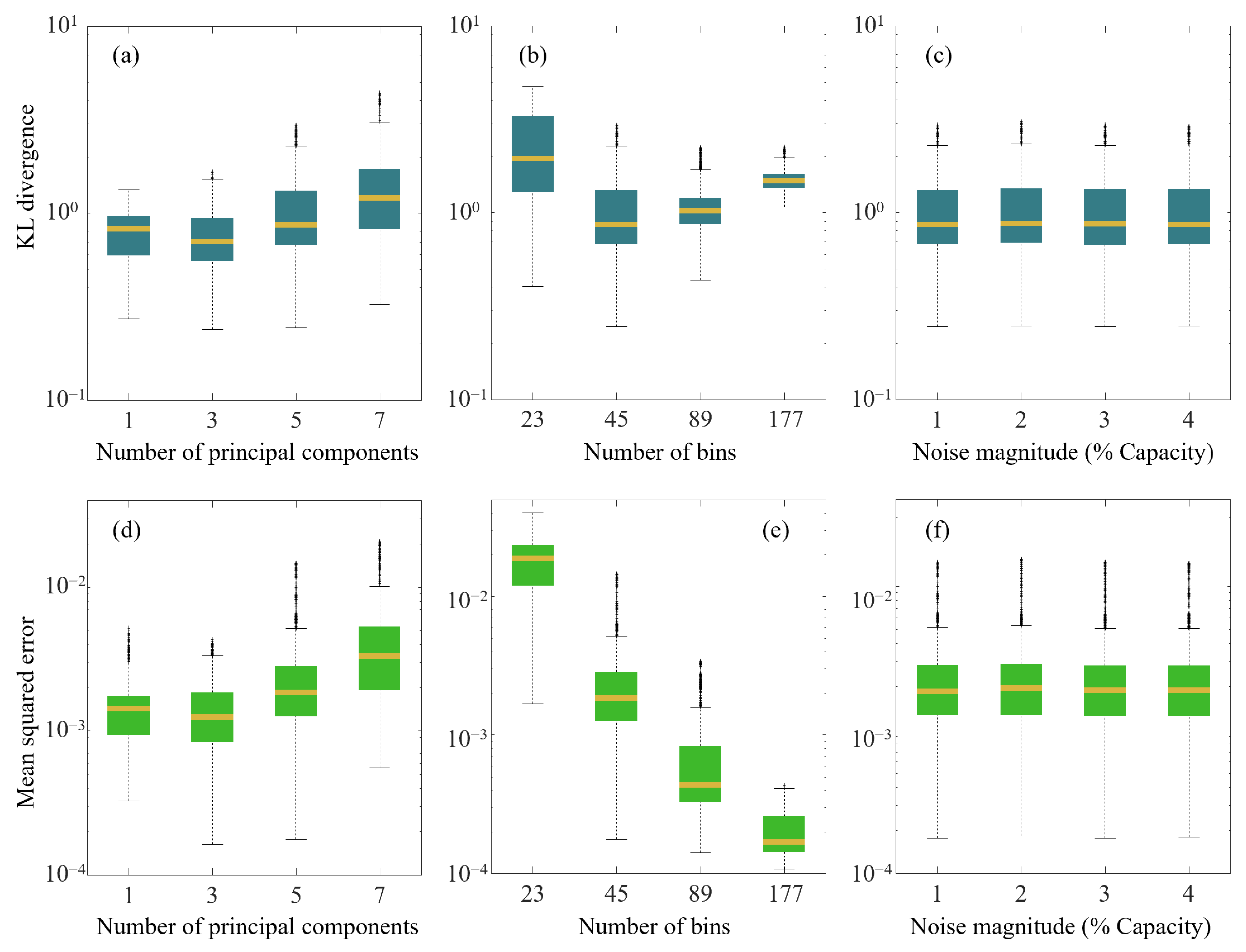
3.5. Sensitivity Analysis

Sensitivity analysis helps evaluate the robustness of the LGP method to design choices and input variations. Thus, we perform a sensitivity analysis focusing on three aspects: the number of principal components retained, the resolution of the capacity histogram (i.e., the number of bins), and the impact of noise in early-cycle data. These experiments are conducted under the same prediction setup used throughout the paper, where the full degradation trajectory of battery RW13 is used for training, and only the first 100 cycles of RW14 are observed for prediction.

We first vary the number of retained principal components in the PCA step. As shown in Figure 6a,d, the model performs best when 3–5 components are kept, balancing dimensionality reduction with information preservation. Including too few components underrepresents structural trends, while including too many can introduce noise, leading to increased prediction error.

The effect of histogram resolution is examined by changing the bin width used to discretize capacity into histograms. Specifically, capacity step sizes of 0.1 Ah, 0.05 Ah, 0.025 Ah, and 0.0125 Ah are used, resulting in 23, 45, 89, and 177 bins, respectively. As shown in Figure 6b,e, increasing the number of bins generally reduces the mean squared error (MSE), as finer resolution enables better matching of local histogram structures. However, a noticeable increase in KL divergence is observed at the highest resolution (177 bins). This discrepancy between MSE and KL behavior arises because KL divergence captures the overall distributional shape rather than localized errors. When the histogram has many bins, many of them may become sparsely populated or empty. Although such sparsity reduces the absolute error in individual bins (hence the lower MSE), even minor deviations in the prediction can accumulate across many bins, leading to amplified differences in the probability distribution and thus a higher KL divergence. Furthermore, retaining a fixed number of principal components in the PCA step may limit the model’s capacity to fully preserve fine-grained histogram features when the number of bins increases. Since PCA reduces dimensionality based on variance concentration, subtle details captured in high-resolution histograms may be compressed or lost. This trade-off between representation resolution and latent feature fidelity may also contribute to the divergence trends observed in Figure 6b,e.

To evaluate robustness to early-cycle measurement uncertainty, we introduce zero-mean Gaussian white noise to the first 100 capacity values of RW14, with the noise standard deviation set to 1%, 2%, 3%, and 4% of the battery initial capacity. As illustrated in Figure 6c,f, the LGP method demonstrates good stability across all tested noise levels. The KL divergence and MSE remain relatively unchanged, suggesting that the model can tolerate moderate levels of input noise without significant degradation in predictive performance.

These results indicate that the LGP framework is resilient to moderate parameter perturbations and input uncertainty, supporting its potential for deployment in real-world battery life prognosis scenarios.

4. Conclusions

This paper presents a Latent GP model for predicting high-dimensional capacity degradation histograms of lithium-ion batteries under dynamic load conditions. The method combines PCA for latent feature extraction with Gaussian Process regression for temporal prediction, enabling accurate distribution forecasting from limited early-cycle data.

We validated the approach using the publicly available NASA PCoE lithium-ion battery dataset. In our experiments, battery RW13 served as the reference cell with full degradation data, while RW14, RW15, and RW16 were used as target cells with only partial data available from the first 100 cycles. The proposed method demonstrated strong predictive performance, with KL divergence consistently remaining below 3 and the median MSE below 0.03. Compared to the conventional Gaussian Process method and a two-layer LSTM baseline, the Latent GP produced more accurate and less scattered forecasts of the capacity degradation histograms. In addition, the model maintained stable prediction accuracy across different starting points for forecasting, including the 1st, 50th, 100th, 200th, and 500th cycle, indicating its robustness under conditions of limited data availability.

Although this study was conducted using the commercial 18,650 cells from the NASA dataset, the proposed method is inherently data-driven and does not rely on specific electrochemical formulations. As long as historical capacity degradation data are available, the Latent GP model can, in principle, be extended to batteries with different cathode chemistries.

Future extensions could incorporate cross-cell correlation modeling, generalization to multi-chemistry datasets, and real-time online learning strategies for deployment in embedded battery management systems.

References

1. Adhikari, N.; Bhandari, R.; Joshi, P. Thermal analysis of lithium-ion battery of electric vehicle using different cooling medium. Appl. Energy 2024, 360, 122781. [Google Scholar] [CrossRef]
2. Balasundar, C.; Sundarabalan, C.K.; Santhanam, S.N.; Sharma, J.; Guerrero, J.M. Mixed Step Size Normalized Least Mean Fourth Algorithm of DSTATCOM Integrated Electric Vehicle Charging Station. IEEE Trans. Ind. Inform. 2023, 19, 7583–7591. [Google Scholar] [CrossRef]
3. Kuzovchikov, S.M.; Zefirov, V.V.; Neudachina, V.S.; Zakharchenko, T.K.; Zybkovets, A.L.; Nikiforov, A.A.; Gusak, D.I.; Reveguk, A.; Kondratenko, M.S.; Yashina, L.V.; et al. Electrolyte refilling as a way to recover capacity of aged lithium-ion batteries. J. Power Sources 2024, 601, 234257. [Google Scholar] [CrossRef]
4. Teliz, E.; López-Vázquez, C.; Díaz, V. Degradation study for 18650 NMC batteries at low temperature. Electrochim. Acta 2024, 475, 143540. [Google Scholar] [CrossRef]
5. You, H.; Wang, X.; Zhu, J.; Jiang, B.; Han, G.; Wei, X.; Dai, H. Investigation of lithium-ion battery nonlinear degradation by experiments and model-based simulation. Energy Storage Mater. 2024, 65, 103083. [Google Scholar] [CrossRef]
6. Li, W.; Li, Y.; Garg, A.; Gao, L. Enhancing real-time degradation prediction of lithium-ion battery: A digital twin framework with CNN-LSTM-attention model. Energy 2024, 286, 129681. [Google Scholar] [CrossRef]
7. Oh, S.; Jeon, A.-R.; Lim, G.; Cho, M.K.; Chae, K.H.; Sohn, S.S.; Lee, M.; Jung, S.-K.; Hong, J. Fast discharging mitigates cathode-electrolyte interface degradation of LiNi0.6Mn0.2Co0.2O2 in rechargeable lithium batteries. Energy Storage Mater. 2024, 65, 103169. [Google Scholar] [CrossRef]
8. Ansari, S.; Ayob, A.; Hossain Lipu, M.S.; Hussain, A.; Md Saad, M.H. Jellyfish optimized recurrent neural network for state of health estimation of lithium-ion batteries. Expert Syst. Appl. 2024, 238, 121904. [Google Scholar] [CrossRef]
9. Xiong, R.; Zhang, Y.; Wang, J.; He, H.; Peng, S.; Pecht, M. Lithium-Ion Battery Health Prognosis Based on a Real Battery Management System Used in Electric Vehicles. IEEE Trans. Veh. Technol. 2019, 68, 4110–4121. [Google Scholar] [CrossRef]
10. Xing, Y.; Ma, E.W.M.; Tsui, K.L.; Pecht, M. An ensemble model for predicting the remaining useful performance of lithium-ion batteries. Microelectron. Reliab. 2013, 53, 811–820. [Google Scholar] [CrossRef]
11. He, W.; Williard, N.; Osterman, M.; Pecht, M. Prognostics of lithium-ion batteries based on Dempster-Shafer theory and the Bayesian Monte Carlo method. J. Power Sources 2011, 196, 10314–10321. [Google Scholar] [CrossRef]
12. Liu, D.; Xie, W.; Liao, H.; Peng, Y. An Integrated Probabilistic Approach to Lithium-Ion Battery Remaining Useful Life Estimation. IEEE Trans. Instrum. Meas. 2015, 64, 660–670. [Google Scholar] [CrossRef]
13. Zhou, Y.; Huang, M. Lithium-ion batteries remaining useful life prediction based on a mixture of empirical mode decomposition and ARIMA model. Microelectron. Reliab. 2016, 65, 265–273. [Google Scholar] [CrossRef]
14. He, W.; Li, Z.; Liu, T.; Liu, Z.; Guo, X.; Du, J.; Li, X.; Sun, P.; Ming, W. Research progress and application of deep learning in remaining useful life, state of health and battery thermal management of lithium batteries. J. Energy Storage 2023, 70, 107868. [Google Scholar] [CrossRef]
15. Lyu, C.; Lai, Q.; Ge, T.; Yu, H.; Wang, L.; Ma, N. A lead-acid battery’s remaining useful life prediction by using electrochemical model in the Particle Filtering framework. Energy 2017, 120, 975–984. [Google Scholar] [CrossRef]
16. Ren, Y.; Tang, T.; Xia, Q.; Zhang, K.; Tian, J.; Hu, D.; Yang, D.; Sun, B.; Feng, Q.; Qian, C. A data and physical model joint driven method for lithium-ion battery remaining useful life prediction under complex dynamic conditions. J. Energy Storage 2024, 79, 110065. [Google Scholar] [CrossRef]
17. Khaleghi, S.; Hosen, M.S.; Van Mierlo, J.; Berecibar, M. Towards machine-learning driven prognostics and health management of Li-ion batteries. A comprehensive review. Renew. Sustain. Energy Rev. 2024, 192, 114224. [Google Scholar] [CrossRef]
18. Alsuwian, T.; Ansari, S.; Zainuri, M.A.A.M.; Ayob, A.; Hussain, A.; Lipu, M.H.; Alhawari, A.R.; Almawgani, A.; Almasabi, S.; Hindi, A.T. A review of expert hybrid and co-estimation techniques for SOH and RUL estimation in battery management system with electric vehicle application. Expert Syst. Appl. 2024, 246, 123123. [Google Scholar] [CrossRef]
19. Huang, Y.; Zhang, P.; Lu, J.; Xiong, R.; Cai, Z. A transferable long-term lithium-ion battery aging trajectory prediction model considering internal resistance and capacity regeneration phenomenon. Appl. Energy 2024, 360, 122825. [Google Scholar] [CrossRef]
20. Zhao, H.; Meng, J.; Peng, Q. Early perception of Lithium-ion battery degradation trajectory with graphical features and deep learning. Appl. Energy 2025, 381, 125214. [Google Scholar] [CrossRef]
21. Yang, Y.; Yang, J.; Wu, X.; Fu, L.; Gao, X.; Xie, X.; Ouyang, Q. Battery pack capacity prediction using deep learning and data compression technique: A method for real-world vehicles. J. Energy Chem. 2025, 106, 553–564. [Google Scholar] [CrossRef]
22. Du, J.; Zhang, C.; Li, S.; Zhang, L.; Zhang, W. Two-stage prediction method for capacity aging trajectories of lithium-ion batteries based on Siamese-convolutional neural network. Energy 2024, 295, 130947. [Google Scholar] [CrossRef]
23. Zafar, M.H.; Mansoor, M.; Houran, M.A.; Khan, N.M.; Khan, K.; Moosavi, S.K.R.; Sanfilippo, F. Hybrid deep learning model for efficient state of charge estimation of Li-ion batteries in electric vehicles. Energy 2023, 282, 128317. [Google Scholar] [CrossRef]
24. Xiang, Y.; Fan, W.; Zhu, J.; Wei, X.; Dai, H. Semi-supervised deep learning for lithium-ion battery state-of-health estimation using dynamic discharge profiles. Cell Rep. Phys. Sci. 2024, 5, 101763. [Google Scholar] [CrossRef]
25. Fan, Y.; Xiao, F.; Li, C.; Yang, G.; Tang, X. A novel deep learning framework for state of health estimation of lithium-ion battery. J. Energy Storage 2020, 32, 101741. [Google Scholar] [CrossRef]
26. Bole, B.; Kulkarni, C.S.; Daigle, M. Adaptation of an electrochemistry-based Li-ion battery model to account for deterioration observed under randomized use. In PHM 2014—Proceedings of the Annual Conference of the Prognostics and Health Management Society 2014; Prognostics and Health Management Society: New York, NY, USA, 2014; pp. 502–510. [Google Scholar]
27. Lu, J.; Xiong, R.; Tian, J.; Wang, C.; Hsu, C.-W.; Tsou, N.-T.; Sun, F.; Li, J. Battery degradation prediction against uncertain future conditions with recurrent neural network enabled deep learning. Energy Storage Mater. 2022, 50, 139–151. [Google Scholar] [CrossRef]
28. Lu, J.; Xiong, R.; Tian, J.; Wang, C.; Sun, F. Deep learning to predict battery voltage behavior after uncertain cycling-induced degradation. J. Power Sources 2023, 581, 233473. [Google Scholar] [CrossRef]
29. Lu, J.; Xiong, R.; Tian, J.; Wang, C.; Sun, F. Deep learning to estimate lithium-ion battery state of health without additional degradation experiments. Nat. Commun. 2023, 14, 2760. [Google Scholar] [CrossRef]
30. Lombardo, T.; Duquesnoy, M.; El-Bouysidy, H.; Årén, F.; Gallo-Bueno, A.; Jørgensen, P.B.; Bhowmik, A.; Demortière, A.; Ayerbe, E.; Alcaide, F.; et al. Artificial Intelligence Applied to Battery Research: Hype or Reality? Chem. Rev. 2022, 122, 10899–10969. [Google Scholar] [CrossRef]
31. Nobre, J.; Neves, R.F. Combining Principal Component Analysis, Discrete Wavelet Transform and XGBoost to trade in the financial markets. Expert Syst. Appl. 2019, 125, 181–194. [Google Scholar] [CrossRef]
32. Deringer, V.L.; Bartók, A.P.; Bernstein, N.; Wilkins, D.M.; Ceriotti, M.; Csányi, G. Gaussian Process Regression for Materials and Molecules. Chem. Rev. 2021, 121, 10073–10141. [Google Scholar] [CrossRef] [PubMed]
33. Valverde, J.M.; Tohka, J. Region-wise loss for biomedical image segmentation. Pattern Recognit. 2023, 136, 109208. [Google Scholar] [CrossRef]
34. Van Erven, T.; Harrëmos, P. Rényi divergence and kullback-leibler divergence. IEEE Trans. Inf. Theory 2014, 60, 3797–3820. [Google Scholar] [CrossRef]
35. Gal, Y.; Ghahramani, Z. Dropout as a Bayesian approximation. arXiv 2015, arXiv:1506.02157. [Google Scholar] [CrossRef]
Figure 1. Overview of the proposed prediction framework.
Energies 18 03503 g001
Figure 2. Scatter plot of battery discharge capacity degradation under dynamic load: (a) RW13; (b) RW14; (c) RW15; (d) RW16.
Energies 18 03503 g002
Figure 3. Prediction results on RW14, RW15, and RW16 using the proposed method. (a,e,i): Measured histograms. (b,f,j): Predicted histograms. (c,g,k,d,h,l): KL divergence and MSE boxplots from cycle 100 onward.
Energies 18 03503 g003
Figure 4. Predictions on RW14 using RW13 as the source, starting from cycle 100. (ad): Results from LSTM, MC Dropout LSTM, standard GP, and Latent GP. (eh): Corresponding KL divergence and MSE.
Energies 18 03503 g004
Figure 5. KL divergence (a) and MSE (b) for predictions starting at cycles 1, 50, 100, 200, and 500.
Energies 18 03503 g005
Figure 6. Sensitivity analysis: (a,d) impact of number of retained principal components; (b,e) impact of capacity histogram resolution (bin count); (c,f) impact of early-cycle capacity noise level. Top row: KL divergence; bottom row: MSE.
Energies 18 03503 g006
Disclaimer/Publisher’s Note: The statements, opinions and data contained in all publications are solely those of the individual author(s) and contributor(s) and not of MDPI and/or the editor(s). MDPI and/or the editor(s) disclaim responsibility for any injury to people or property resulting from any ideas, methods, instructions or products referred to in the content.