Abstract
Addressing the problem that energy supply and load demand cannot be matched due to the difference in inertia effects among multiple energy sources, and taking into account the thermoelectric load, this paper designs a two-stage operation optimization model of IES considering multi-dimensional thermal inertia and constructs an intelligent adaptive solution method based on a time scale-model base. Validation is conducted through an arithmetic example. Scenario 2 has 15.3% fewer CO2 emissions than Scenario 1, 19.7% less purchased electricity, and 20.0% less purchased electricity cost. The optimal algorithm for the day-ahead phase is GA, and the optimal algorithm for the intraday phase is PSO, which is able to produce optimization results in a few minutes.
1. Introduction
At present, China’s power transformation is at a critical inflection point from simple renewable energy substitution to a more complex integrated energy system (IES) [1]. Compared with the traditional independent operation of multiple energy systems, IES can realize the complementary advantages between multiple energy sources, energy flow and mutual aid, and plays a significant role in improving the energy utilization rate of distribution networks, improving system operation flexibility and reducing environmental pollution [2]. However, there is a difference in inertial impacts between these multiple energy resources, and this variability leads to complexity and uncertainty in energy system operation. The operation of multi-energy systems becomes particularly complex when thermoelectric loads are considered.
The thermal inertia problem due to the different energy transfer characteristics of thermoelectric media poses a challenge to the coordinated operation of integrated energy systems. Therefore, studies addressing the thermal inertia problem are important for improving the flexibility of integrated energy systems and clean energy consumption. CHEN et al. [3] utilized hydrogen and thermal inertia synergies to enhance hydrogen-enriched compressed natural gas and IES operational efficiency. ZHANG et al. [4] employed a standalone solar–wind–natural gas-based integrated energy system to explore the relationship between uncertainty, thermal inertia, and user comfort. WANG et al. [5] proposed a unified gas-thermal inertia model considering convenient utilization to verify the economic and environmental friendliness of uniform gas thermal inertia participation in power shortage support. LI et al. [6] proposed a novel optimal scheduling model based on Chance Constrained Programming, which takes into account the thermal inertia of buildings and aims to minimize the minimum generation cost. LI et al. [7] proposed a two-stage capacity optimization allocation method considering thermal inertia and user satisfaction, aiming to reduce the total annual cost and enhance clean energy consumption through optimal equipment scheduling. SUN et al. [8] established a multiple thermal inertia model for solid thermal storage electric boilers, heat networks, and buildings, and proposed an improved two-stage robust optimal scheduling method considering thermal inertia uncertainty. WANG et al. [9] proposed an optimal scheduling method considering the thermal inertia of buildings in different heat regulation modes, which reduces the operating costs by modelling the hydraulic–thermal coupling of district heating networks. ZHANG et al. [10] proposed a stochastic optimal scheduling method for combined electric and thermal systems considering the thermal inertia of the district heating network, and established a linearized model of an advanced adiabatic compressed air energy storage plant and a model of the thermal inertia of the heating pipeline network.
Currently, research into the operation optimization of integrated energy systems mainly considers economic, environmental, and energy efficiency aspects. And the multi-objective solution algorithm has certain limitations. SUN et al. [11] proposed a hybrid algorithm called Non-Dominated Sorting Beluga Whale Optimization, which combines the Non-Dominated Sorting Genetic Algorithm II and the Beluga Whale Optimization to solve the model optimization problem. LUO et al. [12] used a coupled dynamic genetic algorithm to output thermal optimization results for an urban integrated power system. XU et al. [13] proposed a multi-objective particle swarm optimization by multi-strategy improvements to solve the multi-objective hybrid energy storage optimization configuration model. WANG et al. [14] considered the electrical and thermal load demand of decentralized integrated energy systems in rural areas, with the dual objective of improving the economy and environmental friendliness of the integrated heating system. MAZOUZI et al. [15] proposed an integrated energy management strategy for fuel cell hybrid electric vehicles by optimizing fuzzy logic parameters with a genetic algorithm, effectively improving system efficiency and performance. ZHANG et al. [16] proposed a multi-objective hierarchical solution method based on the Fishhawk optimization algorithm, which synchronously improves operator revenue, reduces subscriber cost sentiments, and reduces net load fluctuations through a three-layer co-optimization framework. SU et al. [17] employed Latin hypercubic sampling and non-dominated sorting genetic algorithms to propose a multi-objective optimal planning methodology that takes into account source-load uncertainty and achieves a reduction in total annual cost and carbon dioxide emission, and reliability enhancement. SHAFIEI et al. [18] proposed a multi-objective optimization framework incorporating a gravitational search algorithm to achieve multi-objective co-optimization for system resilience enhancement, carbon emission reduction, and operational efficiency improvement by coordinating renewable energy, energy storage, and demand response. LIU et al. [19] proposed a variable step size approximation solution method to achieve multi-objective synergistic optimization for economy, environmental protection, and efficiency. WU et al. [20] employed a multi-objective capacity optimization allocation method combining a non-dominated sorting genetic algorithm with a similar sorting method for ideal solutions for a system solution. LI et al. [21] proposed a three-phase synergistic operation method for park-level integrated energy system clusters based on a large language model prediction and a dynamic green power pricing strategy, and established a multi-objective low-carbon economic optimization operation model.
The main differences compared to previous studies are as follows, as Table 1.

Table 1.
Summary of the comparison between this paper and previous studies.
- (1)
- The current research on thermal inertia focuses on electric and thermal systems; there is a lack of coordination between the grid and the thermal network, and only a single inertia of the thermal network system is considered, which affects the capacity of renewable energy consumption and the system operation economy.
- (2)
- The current research on multidimensional thermal inertia mainly relies on single-phase optimization, neglecting the research on day-ahead-intraday two-phase optimization, and only from the source, network, and load unilateral, which is not able to improve the energy efficiency as a whole.
- (3)
- Most of the existing comprehensive energy system operation optimization models consider economy and energy efficiency separately, and there is a lack of research into comprehensive consideration of the economy, environment and other multi-objectives. And although the existing multi-objective solution algorithms such as particle swarm and genetic algorithm have been applied in related fields, they still easily fall into the dilemma of local optimization and the difficulty of achieving rapid convergence.
In summary, the main contributions of this paper are as follows:
- (1)
- This paper constructs an IES architecture system incorporating thermal inertia characteristics, develops mechanism modeling based on the thermal dynamic characteristics of the thermal system, and reveals the coupling response mechanism between the thermal network and the energy system.
- (2)
- This paper constructs an IES operation optimization model with multiple thermal inertia coupling, systematically analyzes the multi-dimensional thermal dynamic characteristics such as the heat transfer delay of the pipeline network and the thermal storage effect of buildings, and then designs a synergistic optimization strategy with day-ahead scheduling and intra-day correction.
- (3)
- This paper proposes a multi-timescale algorithm adaptation evaluation mechanism. Aiming at the differences in objective function characteristics and time constraints in different optimization phases, an intelligent preference system based on the algorithm performance feature library is constructed to realize the dynamic matching of optimization models and solution methods.
2. Integrated Energy System in China Considering Thermal Inertia and Its Description
2.1. Architecture of IES Considering Multiple Thermal Inertia
With the diversification of energy demand, electrically and thermally coupled IESs have gradually become a research hotspot, but multi-energy coupling increases the operational complexity and uncertainty. Moreover, most of the previous studies focus on the thermal inertia of a single aspect of the system, and there are fewer studies on the coupling characteristics of interconnections by synthesizing multiple aspects. Therefore, this paper fully exploits the multiple thermal inertia of the system, and guarantees the safety and reliability of operation through coordination and optimization. Multiple thermal inertia is mainly reflected in three aspects; one is the thermal inertia of the heating heat load; the second is the thermal inertia of the energy network transmission; and the third is the thermal inertia of the electro–thermal coupling equipment. Through the mining of energy conversion, energy transmission, the energy demand side and other multifaceted thermal inertia, the complementary mutual aid and flexible scheduling between heterogeneous energy sources of IES can be realized; the specific architecture diagram and thermal inertia are shown in Figure 1. The equipment includes photovoltaic (PV), wind power (WT), an energy storage battery (ESB), thermal energy storage (TES), a gas turbine (GT), and a waste heat boiler (WHB).

Figure 1.
A typical integrated energy system architecture.
As shown in Figure 1, the core framework of model construction and solution in this paper contains four key parts. First, a two-stage optimization model of IES based on multidimensional thermal inertia is established: hourly optimization is performed in the pre-day stage, aiming at economy and environmental protection; 15 min optimization is performed in the intra-day stage, focusing on improving the reliability and stability of the system. Second, a library of solution algorithms containing five algorithms, including the Taboo Search Algorithm and Simulated Annealing Algorithm, is constructed. Third, an algorithm adaptive evaluation system is developed for the multi-timescale scheduling of integrated energy systems considering thermal inertia response, which can adaptively select the most suitable algorithms according to specific scenarios and output system optimization strategies. Fourth, the validity of the model and algorithm is verified through example simulation, and the solution results of the objective function are output.
2.2. Model Construction
2.2.1. Load-Side Demand Response Modeling Considering Thermal Inertia
- Flexible characteristics of electric load [22]
With the development of the electricity market mechanism, the demand response resources on the load side are becoming more and more abundant. According to the user’s response mode, it can be divided into two types: Price-based Demand Response (PDR) and Incentive-based Demand Response (IDR). These two types of demand responses with adjustable characteristics represent the flexibility of the power load. Against the background of the time-of-use electricity price, price is the most direct factor that affects users’ electricity consumption. The demand response of the electricity price type is to guide and change users’ electricity consumption behavior through economic leverage. Even if the change in such a load is only influenced by users’ subjective will, there is no mandatory constraint and the adjustment ability is limited; it is usually regarded as a non-schedulable resource in dispatching, but it can realize the load transfer on the horizontal time axis, which has obvious effects on smoothing the electric load curve and cutting peaks and filling valleys. From this, the elastic matrix of the electricity price is introduced to describe the influence of the price change on the demand change of the electricity price load in a certain period, which can be expressed as follows.
where represents the elasticity index of the electricity price. and respectively represent the electricity consumption before the price-based demand response and the change in the response process. and respectively indicate the difference between the electricity price before and after the price-based demand response. The elastic coefficient matrix of the load electricity price is composed of mutual elastic coefficient and self-elastic coefficient in a certain period of time. and respectively represent the electricity price during period and the change in electricity price after the response. and respectively represent the electricity price during period and the change in electricity price after the response.
The tariff elasticity matrix is a tool to quantify the sensitivity of a customer’s electricity demand to changes in tariffs and describes how changes in tariffs during different time periods affect the relative changes in electricity loads during different time periods, i.e., the percentage change in demand divided by the percentage change in price. In the time-of-use tariff scenario, users’ electricity consumption decisions in one time period are not only affected by the price of electricity in that time period, but also by the price of electricity in other time periods, and, therefore, matrices are needed to describe the complex interrelationships. In this paper, the electricity price elasticity matrix is set to be a 3 × 3 matrix for peak, level, and valley times, which varies according to the actual situation of different scenarios. According to the electricity tariff elasticity matrix, the amount of customer load response under peak, level, and valley time-of-day tariffs can be derived as:
where refers to the electric load transfer after the time-of-use price is implemented, refer to the electric load consumption in peak, average, and valley periods before the time-of-use price is implemented, is the fixed electricity price in the traditional mode, , , are the differences between the fixed electricity price in the traditional mode and the electricity price in peak, flat, and valley periods, respectively.
The calling cost of price-based demand response can be expressed as:
where indicates the price difference before and after the time-sharing response under the time-sharing price.
The incentive demand response strategy refers to the integrated energy system to take reward and punishment measures to encourage and guide users to adjust the call volume, respond in time when the system needs, and mitigate the impact caused by the fluctuation in the system source and load power. Often, an incentive response agreement is signed with the user in advance, in which the basic response capacity, advance notice time, response duration, and compensation fee corresponding to the increased load and punishment corresponding to the user’s failure to participate in the demand response as required need to be stipulated. Therefore, the compensation methods of the incentive demand response can be divided into two categories: capacity compensation and electricity compensation. Capacity compensation means that users can get the capacity compensation fee negotiated in advance as long as they participate in the response, regardless of whether the load is interrupted or not. The power compensation is closely related to the response of the actual call process. In order to stimulate the enthusiasm of users and improve the stability of the system operation, this chapter adopts a multi-stage quotation strategy.
where is the calling cost of the incentive-based demand response, is the unit capacity cost of the incentive demand response, is the total number of users, and is the total number of stages. is the response capacity of the user who responds to the incentive demand, is the unit cost of response power in paragraph in the multi-stage quotation of the incentive demand response, and is the response electric quantity of the user in the stage of the incentive demand response.
- 2.
- Thermal load flexibility characteristics
In the thermal system, heating users usually have the characteristics of fuzzy perception and time delay. Therefore, the temperature becomes an important measure to adjust the heat load demand, especially when the user is in the comfort zone, where the user is less sensitive to temperature changes, so fluctuating back and forth within the upper and lower range of the temperature set value will not have much impact on the user. Secondly, the network characteristics of heating systems will also lead to the thermal inertia effect of heat energy transmission, which makes the heat load adjustment rate slow.
In the centralized heating system in northern China, the heating load is the main factor and the heating process can be roughly expressed as follows: the heat source heats the low-temperature medium (commonly used water as the medium) and converts it into a high-temperature medium, and then transmits it to the heat user terminal through the medium transmission pipe network, and releases heat through the radiator. Then, the cooled medium returns to the low temperature state, and then returns to the heat source through the backwater pipe network, so as to cycle back and forth. The ARMA time series model is introduced to describe the temperature and thermal dynamic characteristics of the heating system, which can be expressed as follows.
where indicates the backwater temperature of the pipe network during the period t, indicate the backwater temperature, water supply temperature, and outdoor temperature of the pipe network during the period , indicates the indoor temperature of the building during the period t, is the order of the ARMA time series model, and , represent the thermal inertia parameters of the heating system under order. In order to further describe the gradual change characteristics of the indoor temperature in buildings, three state variables, namely, indoor temperature, building wall temperature, and building outdoor temperature, are used for the description, which can be expressed as:
where represents the specific heat capacity of indoor air (J/kg·°C), is the instantaneous temperature inside the building, and represent indoor and outdoor temperatures, respectively, indicates the temperature of the building wall, represents the thermal resistance between indoor and outdoor air, indicates the thermal resistance between the building wall and the indoor air, indicates the thermal resistance between the building wall and the outdoor air, indicates the heat released by the radiator, represents the equivalent heating area of the building, and represents the total area of the central heating area.
2.2.2. Network Transmission Modeling Considering Thermal Inertia
The thermal system is divided into a transmission system (primary pipe network) and distribution system (secondary pipe network), in which the primary pipe network connects the heat source with the heat exchange station and transmits the heat of the heat source through hot water, and the secondary pipe network connects the heat exchange station with the heat users, and reasonably distributes the heat energy transmitted to the heat exchange station to the heat users through the heat carrier medium.
The existing thermal system mainly adopts a quality regulation mode and a quantity regulation mode, or both. Because this paper mainly considers the modeling of the primary heating network, quality adjustment is adopted.
As an important part of the heating network, pipeline branch analysis is the premise of heating network analysis. Different from the single process of electric energy flow, in thermodynamics, the transmission of thermal energy is a mixed process of flow process and heat transfer process. The flow process of heat energy involves hydraulic power flow analysis with pressure and mass flow rate as the main factors, and thermal power flow analysis with temperature as the main factors.
For hydraulic analysis, it mainly measures the pressure of each node, the water required by each node, and the flow of each pipeline. The basic model includes a node flow continuity equation, pressure loop equation, and loss equation, as shown below [23]:
where represents the incidence matrix of heating network nodes and pipelines, represents the pipeline flow matrix, represents that flow of people injected into the node, represents the correlation matrix of pipes in a hot water pipe network relative to a heating ring network, represents the loss equation, represents the pressure loss matrix in the heating ring network, represents a coefficient vector, represents the friction coefficient, is the pipe length, m, is the pipe diameter, m, represents the acceleration of gravity, m/s2, represents the density of water, and refers to the time delay.
For thermal analysis, the model is established according to the node temperature fusion and temperature loss as follows.
where and represent the mass flow rate of the pipeline a and the pipeline b, respectively, indicates the outdoor air temperature, and respectively indicate the first section temperature and the end temperature of the pipeline, is the specific heat capacity of water, , respectively refer to the length and inner diameter of the pipeline i, is the temperature loss coefficient, is the hot water transmission delay of the pipeline i, and is the heat transfer efficiency per unit length of the pipeline.
2.2.3. Electrothermal Coupling Modeling Considering Thermal Inertia
- Thermal energy storage
- 2.
- GT
The gas turbine is the core equipment to realize cogeneration, which has the characteristics of fast start–stop and high efficiency. Its input is natural gas and its output is electric energy. In addition, the supporting waste heat recovery device will recycle waste heat and output heat energy. The specific model of gas turbine output is:
where , , , and are the efficiency of the gas turbine in producing various energy sources, is the ratio of exhaust gas regeneration, and the value is taken in the interval [0,1]. and linearization coefficients of energy efficiency characteristics are obtained by linear regression, .
- 3.
- WHB
A waste heat boiler recovers waste heat from the exhaust gas of the gas turbine for heating or refrigeration, and the output heat is:
where is the mass flow of gas passing through the waste heat boiler, , are the specific enthalpies of gas at the inlet and outlet of the waste heat boiler, respectively, and is the thermal efficiency of the waste heat boiler.
3. Operation Optimization Model of IES Based on Multi-Dimensional Thermal Inertia
3.1. Two-Stage Operation Optimization Strategy
Considering that multi-dimensional thermal inertia can respond to users’ needs on different time scales, this paper designs a two-stage operation optimization model of IES considering multi-dimensional thermal inertia to ensure efficient utilization of resources and reduce the economic operation cost of the system. The specific optimization strategy is shown in Figure 2, which is divided into two stages. Hours before the day and 15 min minutes within the day.
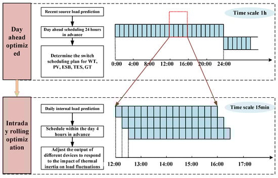
Figure 2.
Operation optimization strategy in day-ahead and intra-day.
In the day-ahead stage, it is scheduled 24 h in advance, with a scheduling time window of 24 h and a time scale of 1 h. In the day-ahead stage, based on an hourly renewable energy output and load forecasting information, variable operation information with a slow response speed and difficult scheduling is given priority, and the on-off state of the controllable equipment in the next 24 h is determined, so as to optimize the comprehensive operation cost.
Intra-day rolling optimization is scheduled 4 h in advance, with a scheduling time window of 4 h and a time scale of 15 min. According to the known output of the system and the actual output of wind power and photovoltaic in the current system, the output of different equipment is adjusted, and in response to the influence of thermal inertia on load fluctuation, the reliability and stability of the system are taken as the main objective function, and the operation cost is considered for optimization.
3.2. Day-Ahead Optimization
In the dispatching stage, the dispatching plan is made 24 h in advance, the time scale is 1 h, and the dispatching window is 24 h. In the day-ahead, based on historical load data, meteorological conditions, and energy price information, the demand for electricity and thermal energy, the output of renewable energy of photovoltaic and wind turbines, and the outdoor temperature of the next day are predicted. According to the predicted results, the optimal dispatching model of the day before yesterday is substituted, and the energy resource supply and equipment output scheme is worked out in advance. Under the conditions of maintaining the balance of energy supply and demand and equipment operation constraints, the demand-side resource adjustment potential is fully exerted, and the peak load and valley load are cut, while the optimal strategy with the lowest operating cost is sought.
3.2.1. Objective Function
In the day-ahead optimization stage of integrated energy systems, the aim is economy and environmental protection, and the energy cost of the system is reduced by reasonably arranging the output plan of units and the operation interval of the controllable load. Therefore, the objective function of the proposed optimization scheduling model is the lowest total operation cost of the integrated energy system, which mainly includes the start-stop cost, operation and maintenance cost, energy purchase cost, penalty cost of abandoning electricity from wind power (WT) and photovoltaic (PV), and carbon emission cost of each unit.
where is the total running cost, is the start-stop cost of each group, CN¥, is the equipment operation and maintenance cost, CN¥, is the energy purchase cost, CN¥, is penalty cost of abandoning wind power and photovoltaic power, CN¥, and is the carbon emission cost, CN¥.
- start-stop cost
The gas turbine switching process includes fuel preheating, system inspection, and start-up sequence and adjustment; the process is long. Defining the on-off state of gas turbine in the day-ahead stage can make a more operable multi-time scale scheduling plan.
where is the start-stop cost of equipment i in the time t, CN¥, is the one-time start-stop cost of equipment i in the system, CN¥, is the start-stop state of the equipment in the time t, is the total number of devices, and is the total number of periods in the whole operation cycle of the system.
- 2.
- Equipment operation and maintenance cost
In the operation process of IES, it is necessary to invest manpower, consumables, technical upgrading, management, and other expenses to ensure the normal operation of the equipment.
where, is the unit operation and maintenance cost of the equipment, CN¥, and is the output power of the equipment i in the time t, kW.
- 3.
- Energy purchase cost
- 4.
- Penalty cost of abandoning wind power and photovoltaic power
- 5.
- Carbon emission cost
According to the typical structure of the IES established in this paper, the carbon emission source comes from the superior power purchase and gas turbine.
where is the carbon emission quota of the system, kg, is the carbon emission quota for purchasing electricity for superiors, kg, is the carbon emission allowance for gas turbines, kg, is power purchased for the higher grid, kW, is the carbon emission quota of gas turbine, kg, is the carbon emission quota per unit electricity purchased by the superior, which is 0.728 kg/(kWh). is the carbon emission quota per unit heat of gas turbine, which is 0.3672 kg/(kWh).
The actual carbon emission of the IES is the sum of the electricity purchased from outside the grid and the gas turbine. According to the emission factor method, the carbon emission model of the system is:
where is the actual carbon emission of IES, kg, is the actual carbon emission of superior power purchase at time t, kg, is the actual carbon emission of the gas turbine at time t, kg, is the carbon emission coefficient of electricity purchased by the superior, which is 1.080 kg/(kwh), is the carbon emission coefficient of the gas turbine, which is taken as 0.6101 kg/(kWh) here.
If the carbon emission of the system exceeds the allocated quota, it is necessary to purchase a carbon emission quota. On the other hand, we can sell the surplus carbon emission quotas and obtain economic benefits. The carbon emission cost model is as follows:
where is the market price of carbon trading, CN¥/kg.
3.2.2. Constraint Condition
The constraints of day-ahead optimization include energy balance constraints, equipment operation constraints, heating network operation constraints, and user satisfaction constraints.
- Energy balance constraint
The integrated energy system in the park contains three energy flows: electricity, heat, and gas. The basis of operation optimization is to ensure the energy consumption of users, so it must meet the multi-load demand of users at all times. The kinds of energy flow balance constraints are as follows.
where , , respectively are the output of the gas turbine, fan, and photovoltaic at time t, kW, are the discharge and charging power of the energy storage battery at time t, kW, , is the actual output value of the electric and heat load, kW, , are the electric and thermal load output prediction error, kW, is the output of the waste heat boiler at time t, kW. Respectively, , are the heat release and charging power of the heat storage tank at time t, kW, is the low calorific value of natural gas, kWh/m3, and is the natural gas volume consumed by the gas turbine at time t, m3.
- 2.
- Equipment operation constraint
The operation of the integrated energy system in the park depends on the call of various energy output equipments to meet the needs of users. Therefore, it is very important to ensure that the equipment runs in a safe range during its operation.
Equipment capacity constraint
where is the lower limit of equipment i output, kW, is the upper limit of output for the equipment , kW, and indicates the on-off state of the equipment at any moment, with 1 indicating the on-state and 0 indicating the off-state.
Operation constraint of energy storage equipment
- Operation constraint of energy storage battery
- Operation constraint of heat storage tank
- 3.
- Operation constraint of heating network
There are many pipes and nodes in the heat network, and the nodes where the pipes intersect represent the mixing of hot water in the pipes. For the same node, if the heat loss at the node is ignored, the temperature of hot water flowing out of the node should be equal to the mixed temperature of hot water flowing into the node in each pipe, and the total flow of the heat medium flowing into and out of the same node is equal. The established node constraint is below.
where , respectively represent the collection of pipes flowing into and out of the same node. At time t, is the hot water quality flow in the J-section pipeline, kg/s.
After considering the thermal inertia of the heating network, it is necessary to set constraints on the inlet temperature and outlet temperature of each pipeline, and set the upper and lower temperature limits of the pipeline according to the indicators formulated by the national heating standard.
where are the inlet and outlet temperature of the heating network node at any moment t, °C, , are the upper and lower limits of hot water injection temperature of the heat network nodes, °C, , are upper and lower limit values of hot water outflow temperature of the heat network nodes, °C.
- 4.
- Demand response constraint
- 5.
- User satisfaction constraint
In the heating system, due to thermal inertia, the storage and release of heat are delayed. In order to ensure the thermal comfort of users, the human thermal comfort index is used to express user satisfaction. We only pay attention to the supply and return water temperature of the heating system, and the human body mainly feels the comfort of the indoor environment by sensing the indoor temperature. Therefore, this paper assumes that the indoor temperature is a variable, ignoring the influence of wind speed and air humidity, assuming that the average radiation temperature of the space is equal to the indoor air temperature, and the other parameters are known constants.
where is the thermal resistance of clothing, m2 c/w, is the comfortable human skin temperature; this paper sets it as 20 °C. is the indoor temperature, °C, and are the upper and lower limits of room temperature, °C.
3.3. Intra-Day Rolling Optimization
In the intra-day dispatching stage, it is necessary to re-forecast the maximum wind and light output, multiple loads of users and outdoor temperature one hour in advance, with the time scale of 5 min and the dispatching window of 4 h. Compared with the accuracy of the forecast made 24 h in advance on the previous day, the accuracy of the forecast made 1 h in advance in the intra-day stage is higher and the error rate is smaller. Therefore, according to the source and load data predicted in the intra-day stage, more accurate equipment output results can be worked out than those in the previous stage, and the equipment output plan can be further improved on the basis of the previous stage.
In the day-ahead dispatching stage, the price-based demand response, the incentive-based demand response, and the on-off state of the gas turbine have been determined, and these values will be introduced into the day-ahead stage in the form of constants. In the intra-day stage, it is necessary to determine the output plan and demand response resources of energy equipment with high importance but poor flexibility, the gas turbine output, and heat output of the waste heat boiler.
3.3.1. Objective Function
The reason why the intra-day scheduling optimization stage can be scrolled is that there is a prediction error between the source and load prediction results of the previous stage and the intra-day stage. In order to balance the output imbalance caused by forecasting error, it is necessary to adjust the output and demand response of the energy equipment on the basis of the equipment operation variable values determined in the previous stage to ensure the stability of the power grid and the balance between supply and demand. Therefore, the lowest operating cost should be considered when the system reliability is the highest at this stage.
The supply reliability index of a comprehensive energy heating system is constructed in the optimization stage of intra-day dispatching; The valve level of energy equipment (VLEE) refers to the impact on the integrated energy system when the energy equipment fails at a certain moment.
where represents the valve stage of the energy equipment, represents the maximum total energy that can be supplied by the rural comprehensive energy heating system after the failure of energy equipment, and represents the maximum total energy that can be supplied by the rural comprehensive energy heating system.
At the same time, the intra-day operation cost should be considered in the intra-day scheduling optimization stage.
3.3.2. Constraint Condition
In the recent stage, the price demand response, the incentive demand response, and the switch state of the gas turbine have been determined, so the relevant constraints are not considered. Except for the above constraints, the remaining constraints are not considered, and the energy balance constraints, equipment operation constraints, heating network operation constraints, demand response constraints, and user satisfaction constraints involved in the intra-day scheduling stage are not described in detail. In addition, some variable values in the intra-day stage are determined in the previous stage, so the existing intra-day–before-day coupling constraints are as follows.
where is the value of the price-based demand response at time t in the previous stage, is time t which can replace the value of electric load demand response in the previous stage, is the value of the demand response of gas load at time t in the previous stage which can be replaced, is the start-up state of the gas turbine at time t in the previous stage, and is the start-up state of the gas boiler at time t in the previous stage.
In addition to the day-ahead and intra-day coupling constraint, the intra-day stage should also meet the intra-day coupling constraint. As the rolling optimization method is adopted in the day, during each rolling process, the first 15 min time scale scheduling plan in the optimized scheduling window will be saved as the actual value of the day operation. And so on, until all the 96 moments of scrolling are completed.
where is the value of gas turbine power generation at time in the intraday stage, kW, is the thermal output of waste heat boiler at moment, kW, and is the value of the load demand response at time that can be reduced at time , kW.
3.4. Construction and Selection of Model Base for Solving Algorithm
In this paper, the algorithm will be selected adaptively according to the different time scales of integrated energy system scheduling considering the thermal inertia response, so as to formulate the equipment scheduling strategy of the integrated energy system accurately. In the operation optimization model, there are a large number of decision variables in the objective function and constraints, some of which are set to 0–1 state variables, and each decision variable needs to consider different time periods, so the optimization model in this paper is a nonlinear programming model. The nonlinear programming problem belongs to the N-P difficult problem in mathematics, and the existing research mainly adopts two algorithms to solve it: a linear solving algorithm and a heuristic algorithm. In this paper, by comparing the characteristics of the linear solution algorithm and heuristic algorithm, the algorithm set is preliminarily screened, five heuristic algorithms are selected, and an intelligent adaptive solution method based on the time scale–model base is constructed. Then, an adaptive evaluation system is constructed for different algorithms in the algorithm library. From the perspectives of convergence time, solution speed and stability, a framework for selecting the optimization algorithms in the day before yesterday considering subjective and objective factors is constructed by combining an analytic hierarchy process and an entropy weight method, and the optimization effects of different algorithms in different optimization stages are evaluated, while the appropriate optimization algorithms in two stages are selected for optimization calculation. The algorithm flow is shown in Figure 3.

Figure 3.
Algorithm flow chart.
3.4.1. Construction of Algorithm Library and Stage Library
In this technology, five algorithms including a tabu search algorithm, a simulated annealing algorithm, a genetic algorithm, a particle swarm optimization algorithm, and a differential optimization algorithm are used to solve the scheduling strategy of the day before the day considering the thermal inertia response comprehensively.
3.4.2. Adaptive Algorithm Evaluation System
According to the performance of different algorithms in different stages, an adaptive evaluation system of algorithms is constructed from four dimensions: convergence time, solution speed, solution accuracy, and stability.
- Convergence time. Refers to the time required for the algorithm to reach the preset convergence standard. The index is quantified by the time value, and the smaller the convergence time is, the higher the index score will be.
- Solving speed. Refers to the total time consumed by the algorithm from the beginning of execution to the conclusion. Quantify the index by time value, and the smaller the solution speed is, the higher the index score will be.
- The objective function value. Refers to the performance level of the objective function value output by the algorithm. The index is quantified by the minimum economic cost, and the smaller the economic cost is, the higher the index score will be.
- Stability. Refers to the characteristics that the output results of the algorithm can remain relatively stable without significant fluctuation or deviation when the input data change and parameters are fine-tuned. Quantify the index by the variance of the objective function value, and the smaller the variance is, the higher the index score will be.
3.4.3. Indicator Empowerment
The results of AHP based on experts’ knowledge and experience are subjective, while the results of the entropy weight method based on information entropy theory are objective. This paper gives consideration to the subjective and objective factors in the evaluation process, adopts an AHP and entropy weight method to give subjective and objective weights, and determines the index combination weight through a weighted average.
where is the combined weight of the index, is the initial weight obtained for AHP, is the modified weight of entropy weight method, and is the correction coefficient for the AHP weight.
3.4.4. Comprehensive Assessment
According to the weight of each index, the comprehensive evaluation scores of different algorithms in different stages are obtained, and the algorithm with the highest comprehensive evaluation score is taken as the solution algorithm in this stage.
where is the comprehensive evaluation score of the algorithm, and is the score of the algorithm under the index.
3.4.5. Solution Steps
The solution steps are shown in Figure 4.
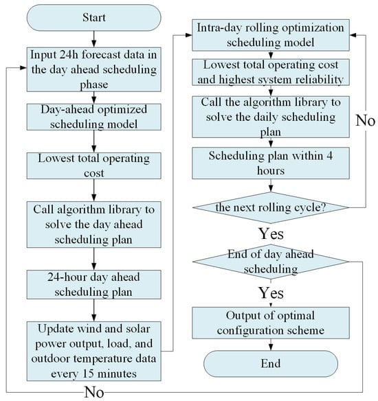
Figure 4.
Solution steps.
- Input system parameters. Real-time load data, weather data, equipment status and historical data, and energy supply.
- Day-ahead scheduling optimization. Based on load forecasting and thermal inertia modeling results, the overall scheduling scheme for a long time period (such as one day) is formulated. Through the above optimization algorithm, a preliminary scheduling scheme is obtained, including the start-stop time of each item of equipment, the charging and discharging plan of the energy storage equipment, etc.
- Intra-day scheduling optimization. According to the new load data, climate change and equipment status, adjust the decision variables in the day-ahead scheduling scheme, dynamically adjust the output of energy storage equipment and electrothermal coupling equipment, optimize the scheduling strategy in real time, and compensate the time lag caused by thermal inertia.
- Update the scheduling strategy. Update the intra-day scheduling strategy based on the optimization results and adjust the charging and discharging mode of the thermal energy storage equipment and the working state of the electrothermal coupling equipment to the best state.
- Rolling optimization. Through continuous feedback and learning, further optimize the scheduling strategy and gradually reduce the lag effect of the system.
4. Example Analysis
4.1. Basic Data
In this paper, a regional integrated energy park is studied to optimize the operation of its integrated energy system on a typical day. QIZHON The equipment in this park and the parameters are specifically shown in Table 2. The devices included in this example are photovoltaic (PV), wind power (WT), combined cooling, heating, and power supply (CCHP) heat pump (HP) energy storage battery (ESB) and thermal energy storage (TES).
Table 2.
System equipment parameters.
According to the wind speed data and light data of this typical day, predicting the output of renewable energy, and the results of renewable energy output are shown in Figure 5.
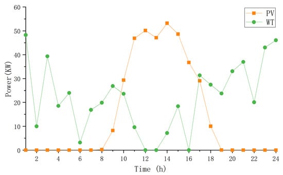
Figure 5.
Renewable energy output results.
In this paper, typical day NG prices and electricity values are shown in Table 3.
Table 3.
Typical day ng prices and electricity values.
4.2. Scenario Setting
Scenario 1: thermal inertia is not considered, and system optimization only considers the scheduling of the power load and controllable load (such as fan, photovoltaic, battery, CCHP, energy storage battery, etc.), ignoring the influence of thermal inertia on thermal energy demand. In this scenario, a two-stage optimal operation model of an integrated energy system is established. Among them, the upper model takes the lowest total operating cost as the objective function to determine the operating state and output of energy equipment in the next 24 h. The lower model takes the lowest total operating cost and the highest system reliability as the objective function to determine the optimal output of the equipment in the next hour.
Scenario 2: thermal inertia is considered, including the time continuity of the thermal load, the influence of thermal inertia on the system response, and the hysteresis of the temperature response of the heat source equipment (such as CCHP, HP and TES). In this scenario, a two-stage optimal operation model considering multiple thermal inertia is established. Among them, the upper model takes the lowest total operating cost as the objective function, and considers the lag effect of the thermal load brought by thermal inertia to determine the operating state and output of the energy equipment in the next 24 h. The lower model takes the lowest total operating cost and the highest system reliability as the objective function, reasonably arranges the unit output and the operation strategy of the thermal energy equipment, reduces the system fluctuation caused by thermal inertia, and ensures the stability and economy of the thermal energy supply.
The two scenario settings are shown in Table 4.
Table 4.
Comparison table of scheme settings.
4.3. Analysis of Operational Result
In order to verify the validity of the method proposed in this paper, different scenarios are set up to explore the influence of multiple thermal inertia on the operation optimization of integrated energy systems. Scenario 1 does not consider multiple thermal inertia, whereas scenario 2 does.
Typical daily loads for this park’s integrated energy system are shown in Figure 6.
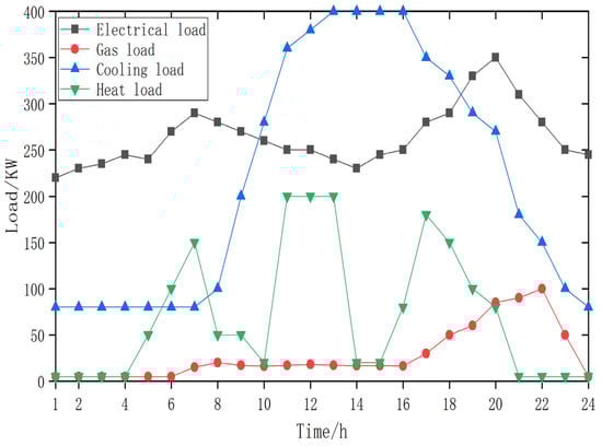
Figure 6.
Typical daily loads for integrated energy systems.
As can be seen from the above figure, the integrated energy system has obvious time-sharing characteristics. The peak energy use occurs at 7:00, 12:00, and 20:00. Among the four types of loads: electric, gas, cold and heat, the average value of the electric load is the highest, close to 300 kW, indicating that the integrated energy system has characteristics centered on electricity.
Figure 7 shows the power and gas purchase curves on a typical day in summer. From the figure, it can be seen that, under the two scenarios, the power and gas purchases of the integrated energy system show obvious time-sharing characteristics.
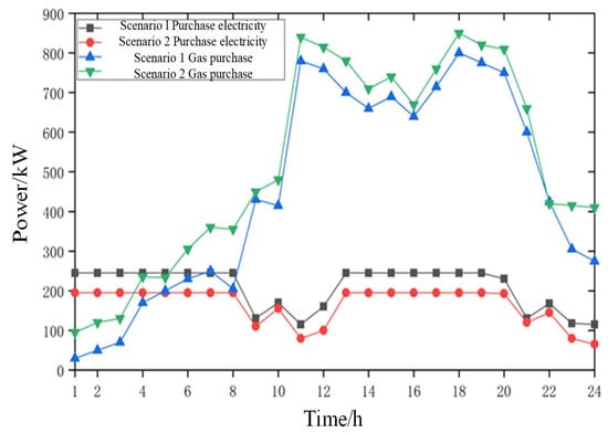
Figure 7.
Electricity and gas purchase curves for a typical summer day.
By comparing scenarios 1 and 2, it can be seen that after considering the multiple thermal inertia, the purchased gas volume of the integrated energy system is larger, with an average increase of 5.2%, and the purchased electricity volume further decreases, with an average decrease of 9.3%.
Figure 8 shows the linear variation in the indoor temperature for different scenarios. The indoor temperature profile considering multiple thermal inertias exhibits significant temperature smoothing characteristics, and its fluctuation amplitude is reduced compared to the scenarios without thermal inertia and with only building thermal inertia, and this temperature stabilization originates from the energy buffering of thermal inertia.
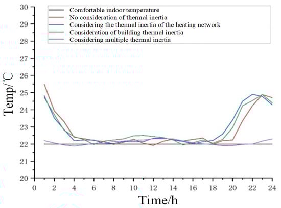
Figure 8.
Line graph of indoor temperature change.
On the one hand, the phase delay of the building body to the hot and cold perturbations significantly suppresses the rate of change of room temperature, and the thermal inertia of the energy network smooths the power fluctuation of the heat source through the time lag of the heat transport of the pipeline workmass to eliminate the heating spikes; on the other hand, the heat energy prefabricated by the electric heating equipment in the valley power hours is temporarily stored through the thermal inertia of the pipeline network and then delayed to be released to the peak load hours by the thermal inertia of the building, which compresses the peak and valley differences of the heat load and reduces heat dissipation losses, as well as the electric heating equipment. The thermal inertia of the electric heating equipment uses the thermal inertia of the equipment to continue the release of residual heat, bridging the energy supply interval.
Figure 9 shows a bar chart of the heating equipment output. It can be seen that compared to the equipment with no thermal inertia and the equipment with only building thermal inertia, the equipment with multiple thermal inertia has less fluctuation in output and smooth output, which can realize the saving of heat energy and reduce carbon emissions.
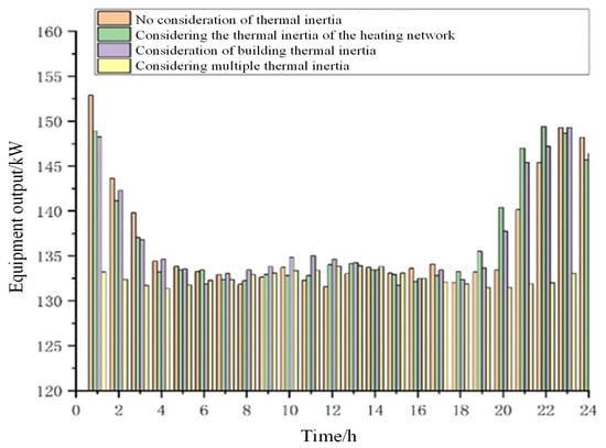
Figure 9.
Heating equipment output bar chart.
Figure 10 and Figure 11 show the electricity supply and demand balance for Scenarios 1 and 2. It can be seen that compared to Scenario 1, Scenario 2 has an overall decrease in the amount of power bought from the grid, an increase in the output of the CCHP, and a decrease in the amount of power used by the heat pumps, which in general improves the energy efficiency and reduces the cost and carbon emissions.

Figure 10.
Scenario 1: Schematic diagram of electricity supply and demand.

Figure 11.
Scenario 2: Schematic diagram of electricity supply and demand.
4.4. Analysis and Discussion
4.4.1. Economic Analysis
As can be seen in Figure 12, in Scenario 1, the power purchase on a typical day is 4961.3 kWh, and the power purchase cost is CN¥ 3766.54. The electricity consumption in Scenario 2 is 3982.4 kWh, and the electricity purchase cost is CN¥ 3013.26. Compared with Scenario 1, the electricity consumption and the electricity purchase cost are reduced by 19.7% and 20.0% in Scenario 2. This may be because the thermal inertia is not considered in Scenario 1, the thermal load response speed of the equipment is fast, and the demand for electric energy fluctuates greatly. It may happen that the demand for electric load cannot be fully met in some time periods, and a large amount of electricity needs to be purchased from the power grid. In addition, the output of some equipment may lead to a waste of electric energy due to excessive adjustment, especially in the peak period of power demand, which may increase the purchase of electricity and the cost of electricity. In the second scenario, because thermal inertia is fully considered, the system can dispatch the load more smoothly and avoid excessive power fluctuations. During the peak period of power demand, the system reduces the dependence on the power grid by arranging the output of heat source equipment in advance. On the whole, the electricity purchase in Scenario 2 is usually lower than that in Scenario 1. By comparing the power purchase price and power purchase price in Scenario 1 and Scenario 2, we can draw the conclusion that the integrated energy system considering thermal inertia has obvious economic advantages. By smoothing the load demand and reasonably dispatching the heat source equipment, the power purchase price and power purchase cost can be significantly reduced, thus improving the overall operating efficiency of the system.
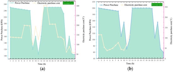
Figure 12.
(a): Power purchase and cost in Scenario 1. (b): Power purchase and cost in Scenario 2.
4.4.2. Carbon Emission Analysis
As shown in Figure 13, both Scenario 1 and Scenario 2 emit more carbon dioxide from CCHP and power purchasing when heating in winter. The difference is that the annual carbon dioxide emission in Scenario 2 is 15.3% less than that in Scenario 1. This is because the energy system in Scenario 1 fails to adjust the load smoothly, especially during peak hours, and may rely on natural gas to generate electricity. In the case of large fluctuations in the heat load demand, the energy utilization efficiency is low and the CO2 emissions are high. In the second scenario, due to the full consideration of thermal inertia, the system can store heat in the low-valley period and adjust the power demand smoothly, which reduces the demand for high-emission power in the peak period and can use renewable energy (such as WT and PV) more efficiently. The load scheduling of the system is more stable and energy waste is avoided, so the overall CO2 emissions are relatively low.
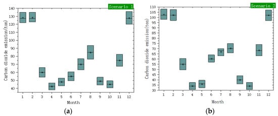
Figure 13.
CO2 emissions in (a) Scenario 1 and (b) Scenario 2.
As can be seen from the schematic diagrams of the power supply and demand scenarios in Scenarios 1 and 2, utilizing the multiple thermal inertia to level or cut the cooling and heating loads enhances the amount of purchased gas and cuts the amount of purchased power, so as to achieve the purpose of reducing the waste of energy and saving the operating costs.
The clean energy consumption ratio and system operation cost data are shown in Table 5.
Table 5.
Comparison of clean energy consumption and operating costs.
Calculation of the basic parameters shows that the operating cost of the integrated energy system without considering multiple thermal inertia in Scenario 1 is CN¥ 25,645.6, while the operating cost of the integrated energy system after considering multiple thermal inertia in Scenario 2 is CN¥ 22,879.8, with a reduction of 12.1%, which fully illustrates the feasibility and validity of the methodology proposed in this paper. At the same time, after considering multiple thermal inertia in Scenario 2, during the peak hours of wind power and PV output, the thermal load demand is reduced, and the output of CCHP units is reduced, which provides space for wind power and PV to be connected to the internet, and improves the consumption capacity.
4.4.3. Performance Analysis of Algorithm
As shown in Figure 14, five algorithms are used for several experiments, and the time (or iteration times) required for each algorithm to reach convergence is recorded. From the point of view of the convergence time, the optimization problem in the previous stage involves a long time span and needs to process a large number of historical data, so the requirement for convergence time is high. Choose Genetic Algorithm (GA) or Aabu Search (TS), and they can find a better solution within a reasonable time. Particle Swarm Optimization (PSO) and Ant Colony Optimization (ACO) have a short convergence time, which is suitable for the intra-day stage and can obtain the optimization results in a few minutes.
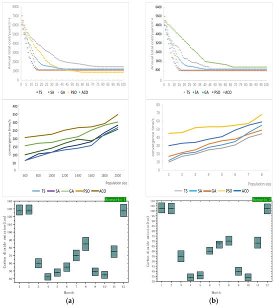
Figure 14.
(a): Iterative curves between Time Scale-Algorithm Library based on day-ahead. (b): Iterative curves between Time Scale-Algorithm Library based on intra-day.
From the point of view of the solving speed, the calculation in the previous stage is large and the solving speed is slow. The optimization time of the intra-day stage is short, so the solution speed of the algorithm is the key. PSO and ACO have a fast solution speed, and can usually complete the optimization within 1–2 min, which is suitable for quickly adjusting the scheduling of the intra-day stage.
Judging from the accuracy of the solution, the accuracy of power and thermal dispatching has a great influence on the system operation, so it is necessary to ensure the accuracy of the solution. In the recent stage, except PSO, all the other four algorithms can reach the approximate global optimal solution. TS and Simulated Annealing Algorithm (SA) are not suitable for real-time scheduling in the day, PSO is easily affected by local optimization, and ACO can give a more accurate solution.
From the stability point of view, GA, PSO and ACO can all reach a more consistent solution in the recent stage. The stability of the algorithm is very important for adjusting the intra-day scheduling strategy to avoid excessive adjustment or unreasonable fluctuation. The particle swarm optimization algorithm and genetic algorithm perform well in stability and are suitable for the intra-day stage.
In a comprehensive selection of the solution algorithm suitable for this case, recently, according to the factors of convergence time, solution accuracy, stability, etc., GA is considered as the best choice, because it can provide higher accuracy and better stability. Although the convergence time is slightly longer, it can find a solution close to the global optimum in complex problems. In the intra-day stage, considering the speed and stability of solution, PSO is the best choice. It can quickly find the near-optimal solution and complete the optimization in a short time, which is suitable for dealing with intra-day dynamic scheduling problems.
5. Conclusions
In order to improve the operation optimization effect of the integrated energy system, this paper puts forward an operation optimization method of an integrated energy system considering multiple thermal inertia. The main research results are summarized as follows:
- (1)
- This paper constructs an IES architecture system that integrates thermal inertia characteristics. By mining the thermal inertia of energy conversion, energy transmission, energy demand side, and other aspects, complementary mutual aid and flexible scheduling between heterogeneous energy sources of IES are realized.
- (2)
- In this paper, an IES operation optimization model with multiple thermal inertia coupling is constructed, and the synergistic optimization strategy of day-ahead scheduling and intra-day correction is designed. The simulation is carried out by comparing scenarios, and the power purchase cost of Scenario 1 is CN¥ 3766.54 and that of Scenario 2 is CN¥ 3013.26, which is a reduction of 20% in power purchase cost, while the annual carbon emission of Scenario 2 is 15.3% less than that of Scenario 1. It effectively improves the operation economy and environmental protection of IES.
- (3)
- This paper constructs an intelligent optimization system based on the algorithm performance feature library. GA is used in the day-ahead phase, which can provide higher accuracy and stronger stability; PSO is used in the intraday phase, which can quickly find the near-optimal solution and complete the optimization in a short time.
At the same time, this paper has some limitations:
- (1)
- The paper puts forward an integrated energy system optimization method based on multiple thermal inertia, but its verification is mainly based on a single typical scenario, lacking a comprehensive analysis of the application effect in different regions or seasons. This may limit the wide applicability of the model in other practical conditions.
- (2)
- In the paper, the operation stability of the system under extreme weather conditions (such as severe cold or a high temperature) and the reliability of the optimization strategy are not deeply discussed, and the research should be more in line with the actual scene requirements.
- (3)
- Furthermore, in the paper, some simplified assumptions are adopted when constructing the multiple thermal inertia model, such as ignoring the influence of some external factors on the dynamic response of the system. This may lead to a reduction in the optimization accuracy of the model in the face of complex multivariable environments in practical application, which limits the universality of the model.
Author Contributions
Conceptualization, H.Z. and M.Z.; methodology, H.Z.; software, H.Z.; validation, X.C., R.F. and H.L.; formal analysis, M.Z.; investigation, H.Z.; resources, H.Z.; data curation, M.Z.; writing—original draft preparation, L.G.; writing—review and editing, L.G.; visualization, J.S.; supervision, J.S.; project administration, H.Z.; funding acquisition, H.Z. All authors have read and agreed to the published version of the manuscript.
Funding
“Science and Technology Project of State Grid” (SGSXDK00DJJS2200316).
Data Availability Statement
Data are unavailable due to privacy.
Conflicts of Interest
All authors were employed by the company State Grid Shanxi Electric Power Company Electric Power Research Institute. The authors declare that the research was conducted in the absence of any commercial or financial relationships that could be construed as a potential conflict of interest.
Nomenclature
| Symbol | |||
| the elasticity index of electricity price | the electricity consumption before the price-based demand response | ||
| the change in the response process | the difference between the electricity price before the price-based demand response | ||
| the difference between the electricity price after the price-based demand response | the elastic coefficient matrix of load electricity price | ||
| self-elastic coefficient | mutual elastic coefficient | ||
| , | the change in electricity price during the period | , | the change in electricity price after the response |
| the electric load transfer after the time-of-use price is implemented | the electric load consumption in peak periods before the time-of-use price is implemented | ||
| the electric load consumption in average periods before the time-of-use price is implemented | the electric load consumption in valley periods before the time-of-use price is implemented | ||
| the fixed electricity price in the traditional mode | the difference between the fixed electricity price in the traditional mode and the electricity price in peak periods | ||
| the difference between the fixed electricity price in the traditional mode and the electricity price in flat periods | the difference between the fixed electricity price in the traditional mode and the electricity price in valley periods | ||
| the calling cost of price-based demand response | the price difference before and after the time-sharing response under the time-sharing price. | ||
| the calling cost of incentive-based demand response | the unit capacity cost of incentive demand response | ||
| U | the total number of users | S | the total number of stages |
| the response capacity of the user | the unit cost of response power in S | ||
| the response electric quantity of the user u in the s stage of the incentive demand response | the backwater temperature of the pipe network during the period t | ||
| the backwater temperature of the pipe network during the period | the water supply temperature of the pipe network during the period | ||
| the outdoor temperature of the pipe network during the period | the indoor temperature of the building during the period t. | ||
| the order of ARMA time series model | the thermal inertia parameters of the heating system under order | ||
| the thermal inertia parameters of the heating system under order | the thermal inertia parameters of the heating system under order | ||
| the thermal inertia parameters of the heating system under order | the thermal inertia parameters of the heating system under order | ||
| the thermal inertia parameters of the heating system under order | the instantaneous temperature inside the building | ||
| the specific heat capacity of indoor air (J/kg·°C) | Indoor temperatures | ||
| outdoor temperatures | the temperature of the building wall | ||
| the thermal resistance between indoor and outdoor air | the thermal resistance between the building wall and the indoor air | ||
| the thermal resistance between the building wall and the outdoor air | the heat released by the radiator | ||
| the equivalent heating area of the building | the total area of central heating area | ||
| the incidence matrix of heating network nodes and pipelines | the pipeline flow matrix | ||
| the flow of people injected into the node | the correlation matrix of pipes in hot water pipe network relative to a heating ring network | ||
| the loss equation | the pressure loss matrix in the heating ring network | ||
| a coefficient vector | the friction coefficient | ||
| the pipe length | the pipe diameter | ||
| the acceleration of gravity | the density of water | ||
| time delay | mass flow rate of the pipeline a | ||
| the mass flow rate of the pipeline b | the outdoor air temperature | ||
| the first section temperature of the pipeline | the end temperature of the pipeline | ||
| the specific heat capacity of water | the length of the pipeline | ||
| the inner diameter of the pipeline | the temperature loss coefficient | ||
| the hot water transmission delay of the pipeline | the heat transfer efficiency per unit length of the pipeline | ||
| the thermal storage capacity at the moment t | the absorption indicating the time t | ||
| the heat release power indicating the time t | the maximum heat storage capacity of the heat storage device | ||
| the maximum heat storage power | the maximum heat release power | ||
| the efficiency of gas turbine in producing various energy sources | the efficiency of gas turbine in producing various energy sources | ||
| the efficiency of gas turbine in producing various energy sources | the efficiency of gas turbine in producing various energy sources | ||
| the ratio of exhaust gas regeneration | linearization coefficients of energy efficiency characteristics | ||
| linearization coefficients of energy efficiency characteristics | the outputs heat of waste heat boiler | ||
| the mass flow of gas passing through the waste heat boiler | the specific enthalpies of gas at the inlet of the waste heat boiler | ||
| the specific enthalpies of gas at the outlet of the waste heat boiler | the thermal efficiency of waste heat boiler | ||
| the total running cost | the start-stop cost of each group | ||
| the equipment operation and maintenance cost | the energy purchase cost | ||
| the penalty cost of abandoning wind power and photovoltaic power | the carbon emission cost | ||
| the start-stop cost of equipment i in the time t | the one-time start-stop cost of equipment i in the system | ||
| the start-stop state of the equipment in the time t | the total number of devices | ||
| the total number of periods in the whole operation cycle of the system | the unit operation and maintenance cost of the equipment | ||
| the output power of the equipment i in the time t | the costs of purchasing electricity from the power grid for the time period system | ||
| the costs of purchasing heat from the heating network for the time period system | the costs of purchasing gas from the grid for the time period system | ||
| the prices of electricity purchased by the system from the market | the prices of heat purchased by the system from the market | ||
| the price of gas purchased by the system from the market | the exchange power of electricity exchange between the system and the power grid during the time period | ||
| the exchange power of electricity exchange between the system and the heat exchange with the heating network during the time period | the exchange power of electricity exchange between the system and gas exchange with the gas grid during the time period | ||
| the predicted power generation of wind power in the time period system | the predicted power generation of photovoltaic in the time period system | ||
| the actual generation power of wind power in the time t | the actual generation power of photovoltaic in the time t | ||
| the penalty coefficient of the system for abandoning wind | the penalty coefficient of the system for abandoning light | ||
| the carbon emission quota of the system | the carbon emission quota for purchasing electricity for superiors | ||
| the carbon emission allowance for gas turbines | power purchased for the higher grid | ||
| the carbon emission quota of gas turbine | the carbon emission quota per unit electricity purchased by the superior | ||
| the carbon emission quota per unit heat of gas turbine | actual carbon emission of the IES | ||
| the actual carbon emission of superior power purchase at time t | the actual carbon emission of the gas turbine at time t | ||
| the carbon emission coefficient of electricity purchased by the superior | the carbon emission coefficient of gas turbine | ||
| the market price of carbon trading | the output of gas turbine at time t | ||
| the output of fan at time t | the output of photovoltaic at time t | ||
| the discharge of the energy storage battery at time t | the charging power of the energy storage battery at time t | ||
| the actual output value of electric | the actual output value of heat load | ||
| the electric output prediction error | the thermal load output prediction error | ||
| the output of waste heat boiler at time t | the heat release of the heat storage tank at time t | ||
| the charging power of the heat storage tank at time t | the low calorific value of natural gas | ||
| the natural gas volume consumed by the gas turbine at time t | the lower limit of equipment i output | ||
| upper limit of output for equipment | the on-off state of the equipment at any moment | ||
| the minimum storage capacity of the battery | the maximum storage capacity of the battery | ||
| the maximum charging power of the battery | the minimum discharge power of the battery | ||
| the minimum heat storage capacity of the heat storage tank | the maximum heat storage capacity of the heat storage tank | ||
| the maximum heating power of the heat storage tank | the minimum heat release power of the heat storage tank | ||
| the collection of pipes flowing into the same node | the collection of pipes flowing out of the same node | ||
| the hot water quality flow in the J-section pipeline | the inlet temperature of the heating network node at any moment t | ||
| the outlet temperature of the heating network node at any moment t | the upper limits of hot water injection temperature of heat network nodes | ||
| the lower limits of hot water injection temperature of heat network nodes | upper limit values of hot water outflow temperature of heat network nodes | ||
| lower limit values of hot water outflow temperature of heat network nodes | the electricity response of the user in response to the incentive demand. | ||
| the thermal resistance of clothing | the comfortable human skin temperature | ||
| indoor temperature | the upper limits of room temperature | ||
| the lower limits of room temperature | the valve stage of energy equipment | ||
| the maximum total energy that can be supplied by the rural comprehensive energy heating system after the failure of energy equipment | the maximum total energy that can be supplied by the rural comprehensive energy heating system | ||
| the value of the price-based demand response at time t in the previous stage | time t can replace the value of electric load demand response in the previous stage | ||
| the value of the demand response of gas load at time t in the previous stage can be replaced | start-up state of the gas turbine at time t in the previous stage | ||
| start-up state of the gas boiler at time t in the previous stage | the value of gas turbine power generation at time in the intraday stage | ||
| the thermal output of waste heat boiler at moment | the value of the load demand response at time that can be reduced at time | ||
| the combined weight of the index | the initial weight obtained for AHP | ||
| the modified weight of entropy weight method | correction coefficient for AHP weight | ||
| the comprehensive evaluation score of the algorithm | the score of the algorithm under the index | ||
| Abbreviation | |||
| IES | integrated energy system | PV | photovoltaic |
| WT | wind power | ESB | energy storage battery |
| TES | thermal energy storage | GT | gas turbine |
| WHB | waste heat boiler | PDR | Price-based Demand Response |
| IDR | Incentive-based Demand Response | ||
| ARMA | Autoregressive Moving Average Model | VLEE | the valve level of energy equipment |
| AHP | Analytic Hierarchy Process | CCHP | combined cooling, heating, and power supply |
| HP | heat pump | NG | Natural Gas |
| GA | Genetic Algorithm | PSO | Particle Swarm Optimization |
| ACO | Ant Colony Optimization | SA | Simulated Annealing Algorithm |
| TS | Tabu Search | ||
References
- Tang, B.-J.; Cao, X.-L.; Li, R.; Xiang, Z.-B.; Zhang, S. Economic and low-carbon planning for interconnected integrated energy systems considering emerging technologies and future development trends. Energy 2024, 302, 131850. [Google Scholar] [CrossRef]
- Wang, M.; Zhang, B.; Su, B.; Wang, M.; Lv, B.; Zhao, Q.; Gao, H. An multi-timescale optimization strategy for integrated energy system considering source load uncertainties. Energy Rep. 2024, 12, 5083–5095. [Google Scholar] [CrossRef]
- Chen, J.; Bie, H.; Wang, J.; Sun, B. Optimization Operation Method for Hydrogen-compressed Natural Gas-Integrated Energy Systems Considering Hydrogen-Thermal Multi-Energy Inertia. Results Eng. 2024, 25, 103652. [Google Scholar] [CrossRef]
- Zhang, J.; Kong, X.; Shen, J.; Sun, L. Day-ahead optimal scheduling of a standalone solar-wind-gas based integrated energy system with and without considering thermal inertia and user comfort. J. Energy Storage 2023, 57, 106187. [Google Scholar] [CrossRef]
- Wang, Q.; Miao, C.; Tang, Y. Power shortage support strategies considering unified gas-thermal inertia in an integrated energy system. Appl. Energy 2022, 328, 120229. [Google Scholar] [CrossRef]
- Li, Y.; Wang, C.; Li, G.; Wang, J.; Zhao, D.; Chen, C. Improving operational flexibility of integrated energy system with uncertain renewable generations considering thermal inertia of buildings. Energy Convers. Manag. 2020, 207, 112526. [Google Scholar] [CrossRef]
- Li, S.; Zhang, J.; He, Y.; Lv, G.; Liu, Y.; Hu, X.; Wang, Z.; Ao, X. Two-Stage capacity allocation optimization method for user-level integrated energy systems considering user satisfaction and thermal inertia. Glob. Energy Interconnect. 2025, 8, 300–315. [Google Scholar] [CrossRef]
- Sun, P.; Teng, Y.; Chen, Z. Robust coordinated optimization for multi-energy systems based on multiple thermal inertia numerical simulation and uncertainty analysis. Appl. Energy 2021, 296, 116982. [Google Scholar] [CrossRef]
- Wang, D.; Zhi, Y.Q.; Jia, H.J.; Hou, K.; Zhang, S.X.; Du, W.; Wang, X.D.; Fan, M.H. Optimal scheduling strategy of district integrated heat and power system with wind power and multiple energy stations considering thermal inertia of buildings under different heating regulation modes. Appl. Energy 2019, 240, 341–358. [Google Scholar] [CrossRef]
- Zhang, Z.; Chen, Y.; Ma, J.; Zhao, D.; Qian, M.; Li, D.; Wang, D.; Zhao, L.; Zhou, M. Stochastic optimal dispatch of combined heat and power integrated AA-CAES power station considering thermal inertia of DHN. Int. J. Electr. Power Energy Syst. 2022, 141, 108151. [Google Scholar] [CrossRef]
- Sun, H.; Cui, Q.; Wen, J.; Kou, L. Optimization and scheduling scheme of park-integrated energy system based on multi-objective Beluga Whale Algorithm. Energy Rep. 2024, 11, 6186–6198. [Google Scholar] [CrossRef]
- Luo, Y.; Yang, S.; Niu, C.; Hua, Z.; Zhang, S. A multi-objective dual dynamic genetic algorithm-based approach for thermoelectric optimization of integrated urban energy systems. Energy Rep. 2024, 12, 4175–4183. [Google Scholar] [CrossRef]
- Xu, X.-F.; Wang, K.; Ma, W.-H.; Wu, C.-L.; Huang, X.-R.; Ma, Z.-X.; Li, Z.-H. Multi-objective particle swarm optimization algorithm based on multi-strategy improvement for hybrid energy storage optimization configuration. Renew. Energy 2024, 223, 120086. [Google Scholar] [CrossRef]
- Wang, Y.; Guo, L.; Ma, Y.; Han, X.; Xing, J.; Miao, W.; Wang, H. Study on operation optimization of decentralized integrated energy system in northern rural areas based on multi-objective. Energy Rep. 2022, 8, 3063–3084. [Google Scholar] [CrossRef]
- Mazouzi, A.; Hadroug, N.; Alayed, W.; Hafaifa, A.; Iratni, A.; Kouzou, A. Comprehensive optimization of fuzzy logic-based energy management system for fuel-cell hybrid electric vehicle using genetic algorithm. Int. J. Hydrog. Energy 2024, 81, 889–905. [Google Scholar] [CrossRef]
- Zhang, G.; Chen, H.; Yang, L.; Gao, J.; Ji, B.; Li, L. Multi-objective optimization of an integrated energy system with shared energy storage. J. Build. Eng. 2025, 111, 113176. [Google Scholar] [CrossRef]
- Su, Z.; Zheng, G.; Wang, G.; Mu, Y.; Fu, J.; Li, P. Multi-objective optimal planning study of integrated regional energy system considering source-load forecasting uncertainty. Energy 2025, 319, 134861. [Google Scholar] [CrossRef]
- Shafiei, K.; Seifi, A.; Hagh, M.T. A novel multi-objective optimization approach for resilience enhancement considering integrated energy systems with renewable energy, energy storage, energy sharing, and demand-side management. J. Energy Storage 2025, 115, 115966. [Google Scholar] [CrossRef]
- Liu, S.; Han, S.; Tian, J.; Rong, N. A multi-objective optimization scheduling approach of integrated energy system considering the exergy efficiency using the variable step-size approximation method. Energy 2024, 311, 133370. [Google Scholar] [CrossRef]
- Wu, K.; Jiang, M.; Huang, Y.; Dai, Z.; Wang, X.; Duan, Z.; Wang, Y.; Li, G. Optimization of multi-objective capacity allocation and performance analysis for integrated energy systems considering hydrogen storage. Energy 2025, 325, 136160. [Google Scholar] [CrossRef]
- Li, Y.; Hu, W.; Zhang, F.; Li, Y. Multi-objective collaborative operation optimization of park-level integrated energy system clusters considering green power forecasting and trading. Energy 2025, 319, 135055. [Google Scholar] [CrossRef]
- Kansal, G.; Tiwari, R. Elasticity modelling of price-based demand response programs considering customer’s different behavioural patterns. Sustain. Energy Grids Netw. 2023, 36, 101244. [Google Scholar] [CrossRef]
- Wang, Y.; Li, Y.; Zhang, Y.; Xu, M.; Li, D. Optimized operation of integrated energy systems accounting for synergistic electricity and heat demand response under heat load flexibility. Appl. Therm. Eng. 2024, 243, 122640. [Google Scholar] [CrossRef]
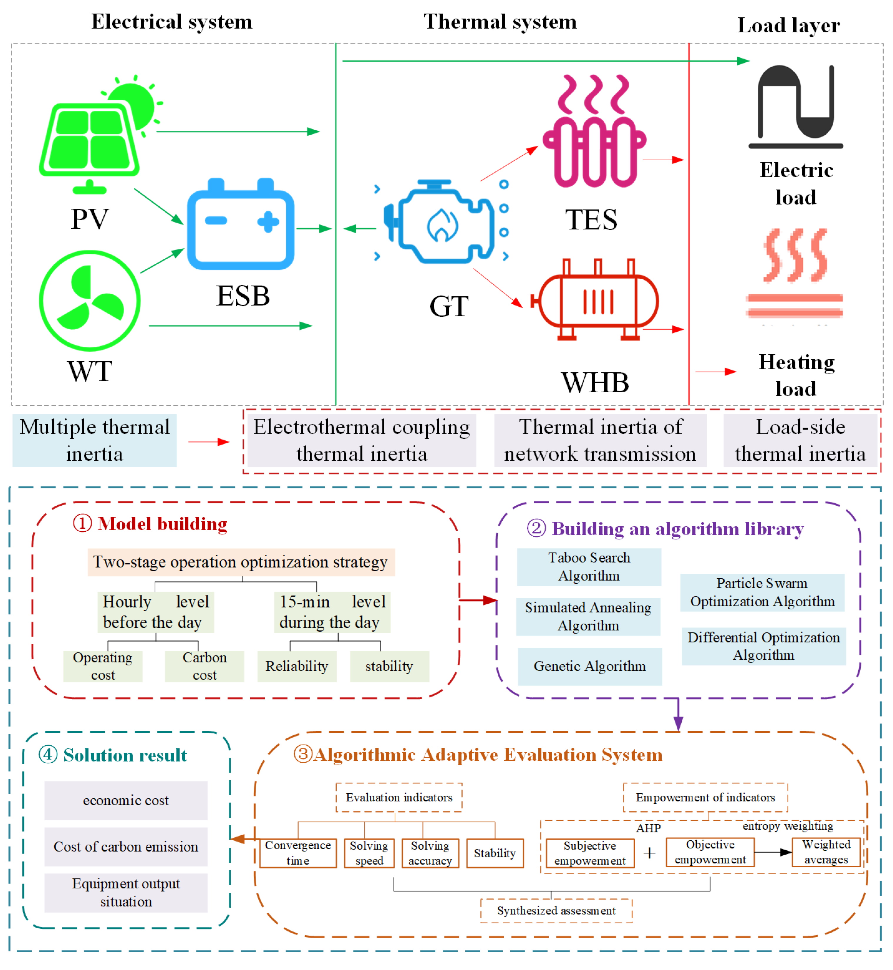
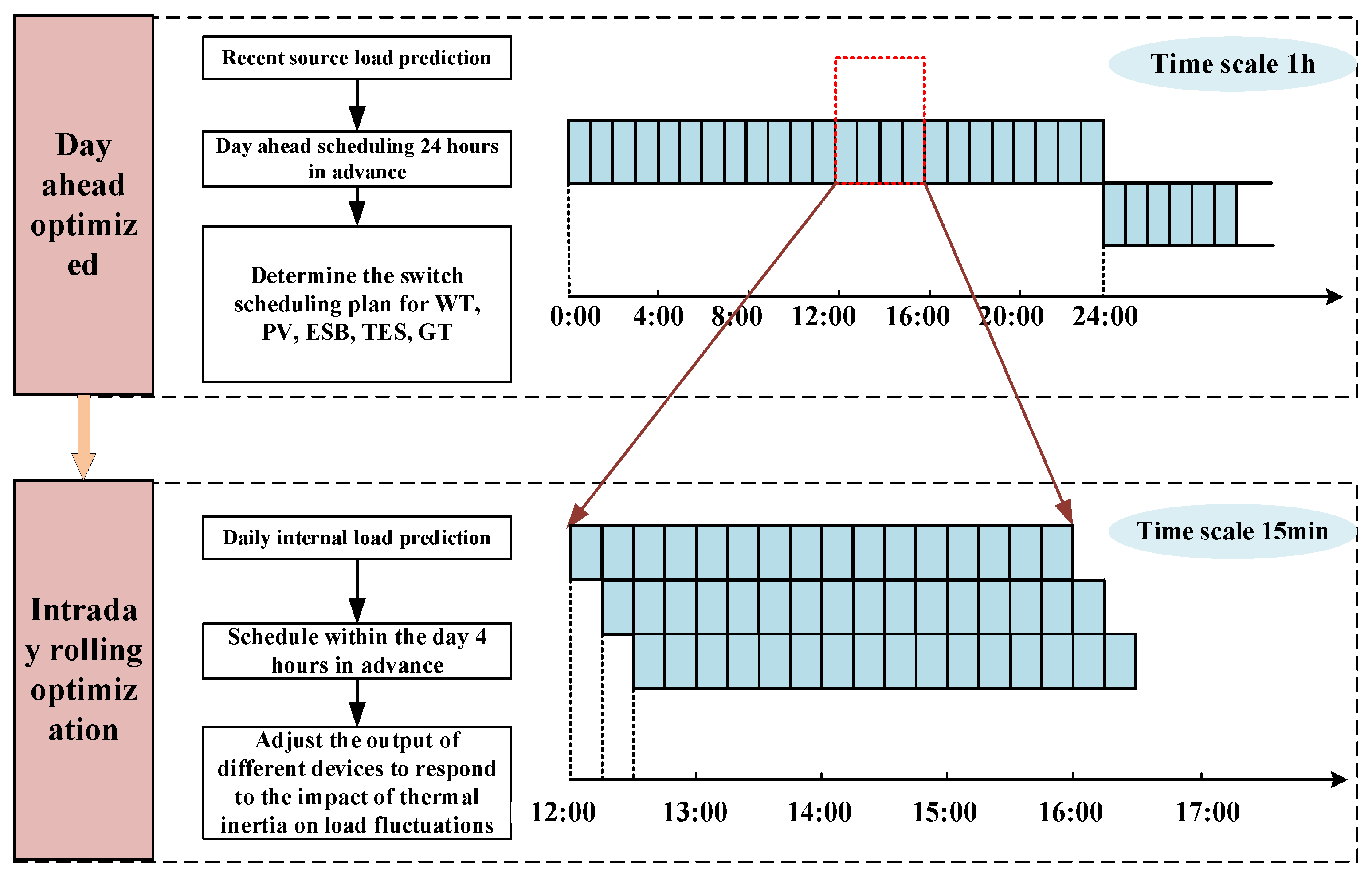
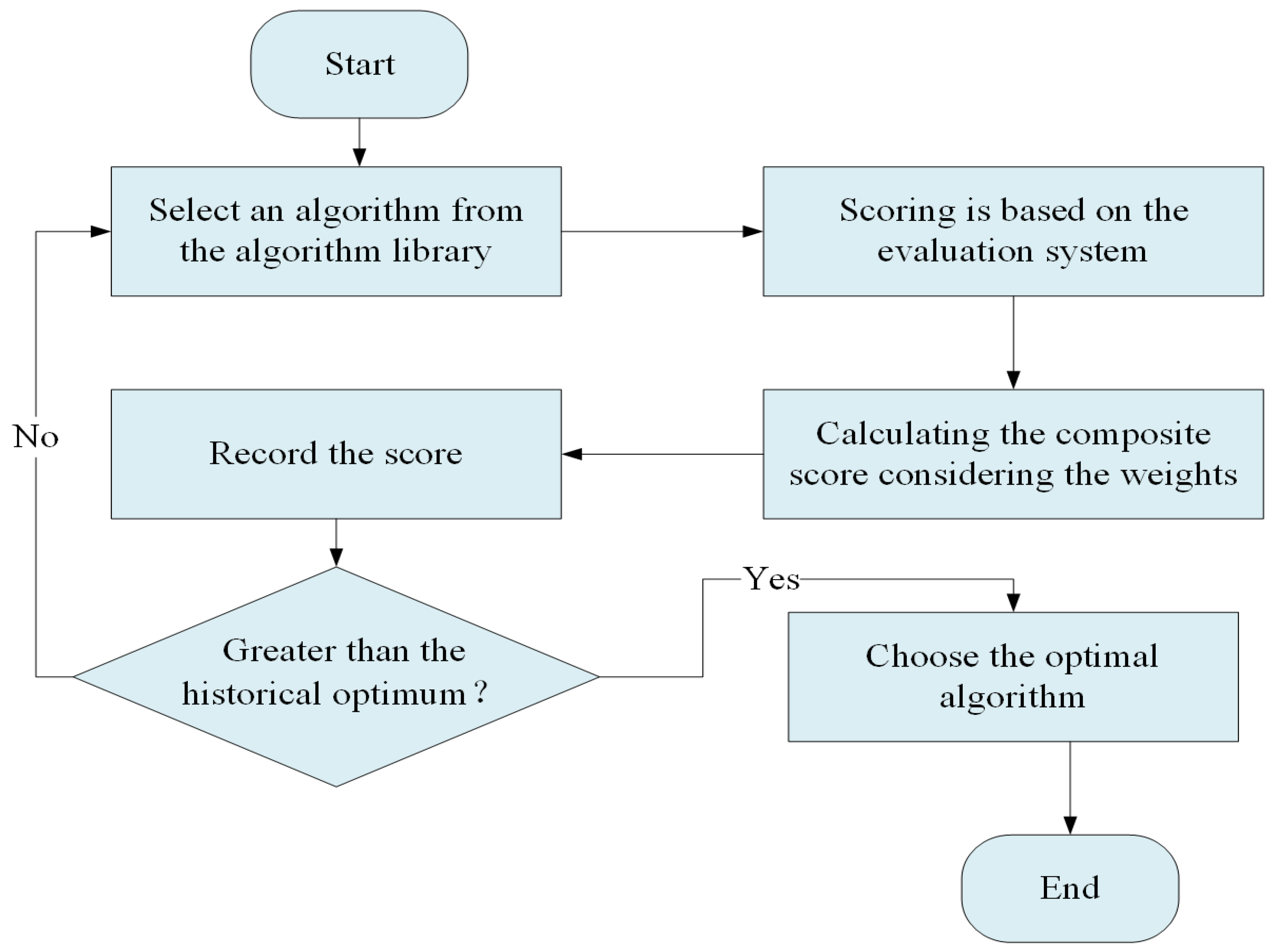
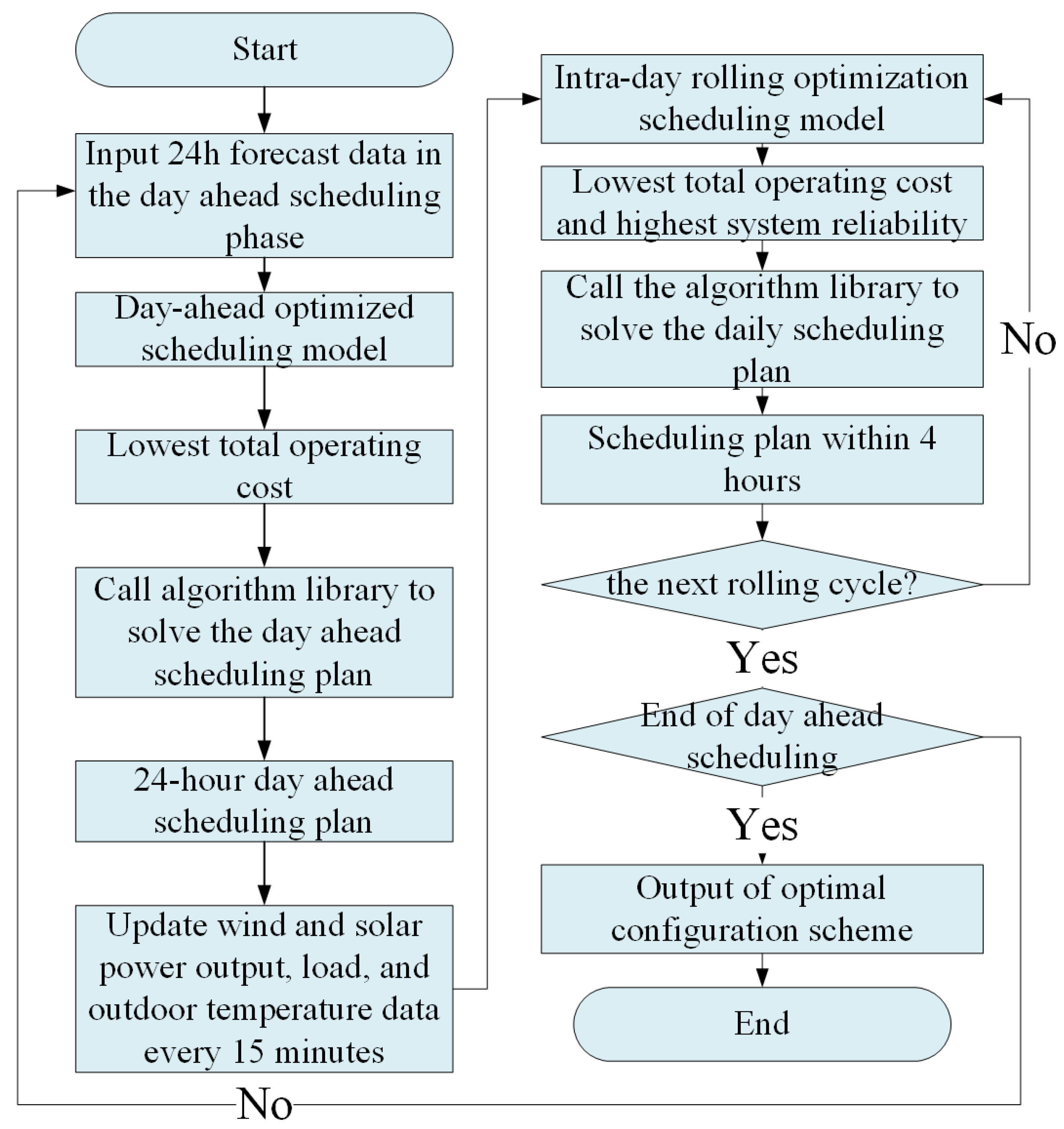
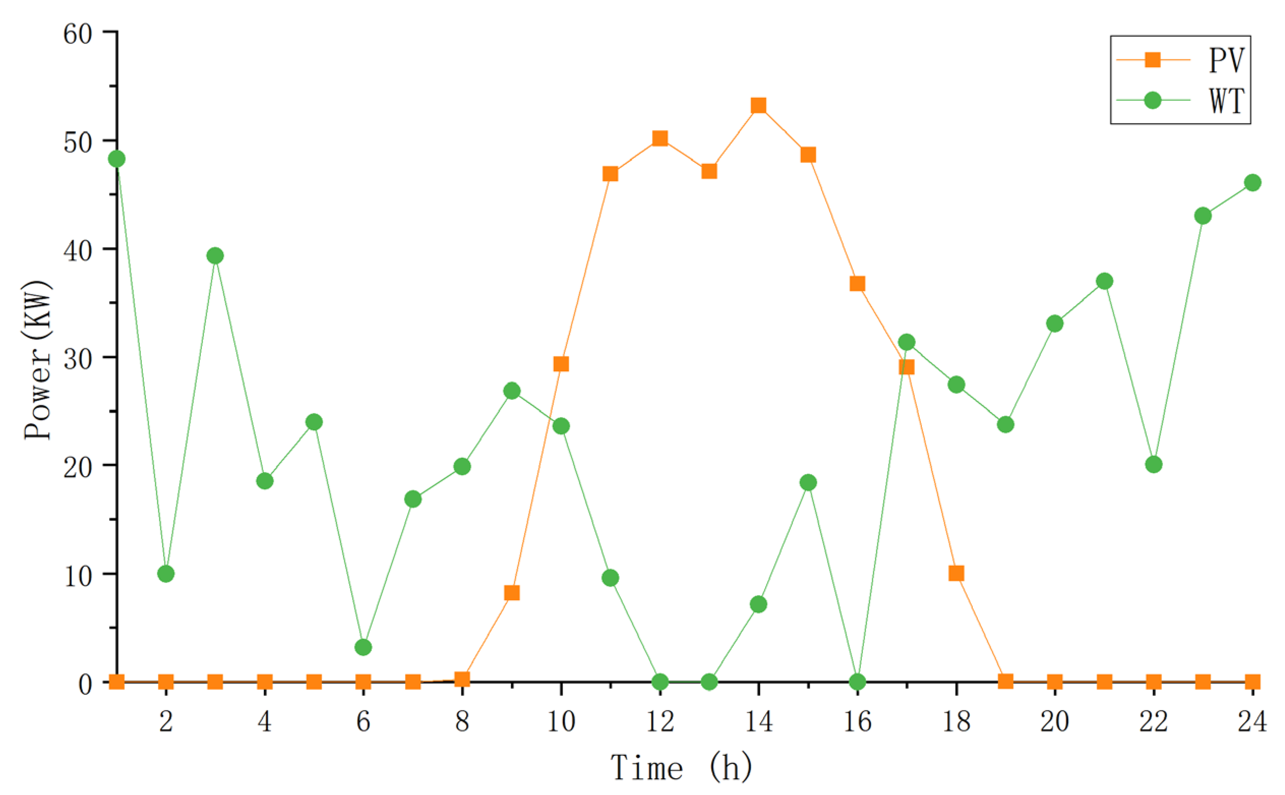
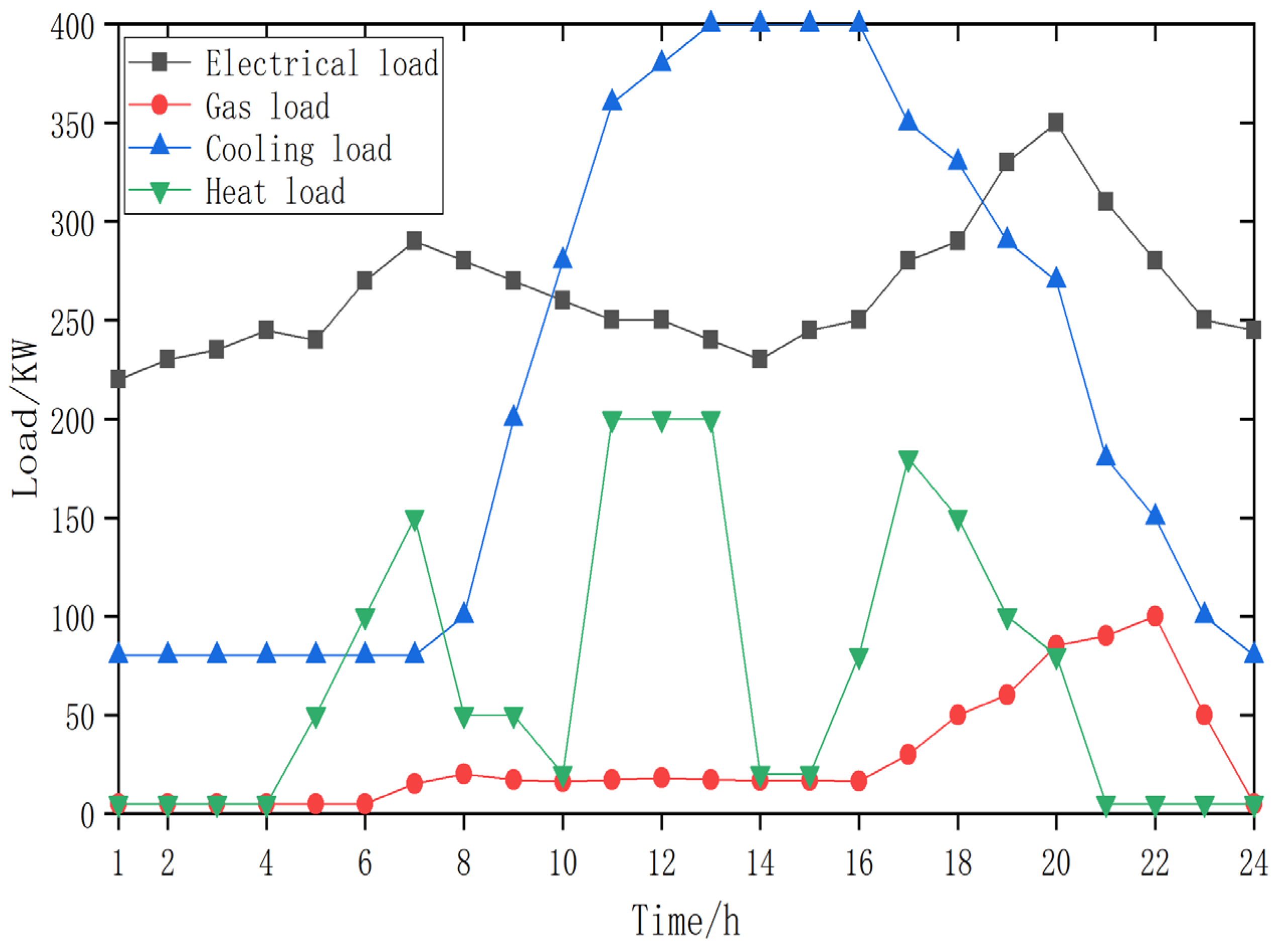
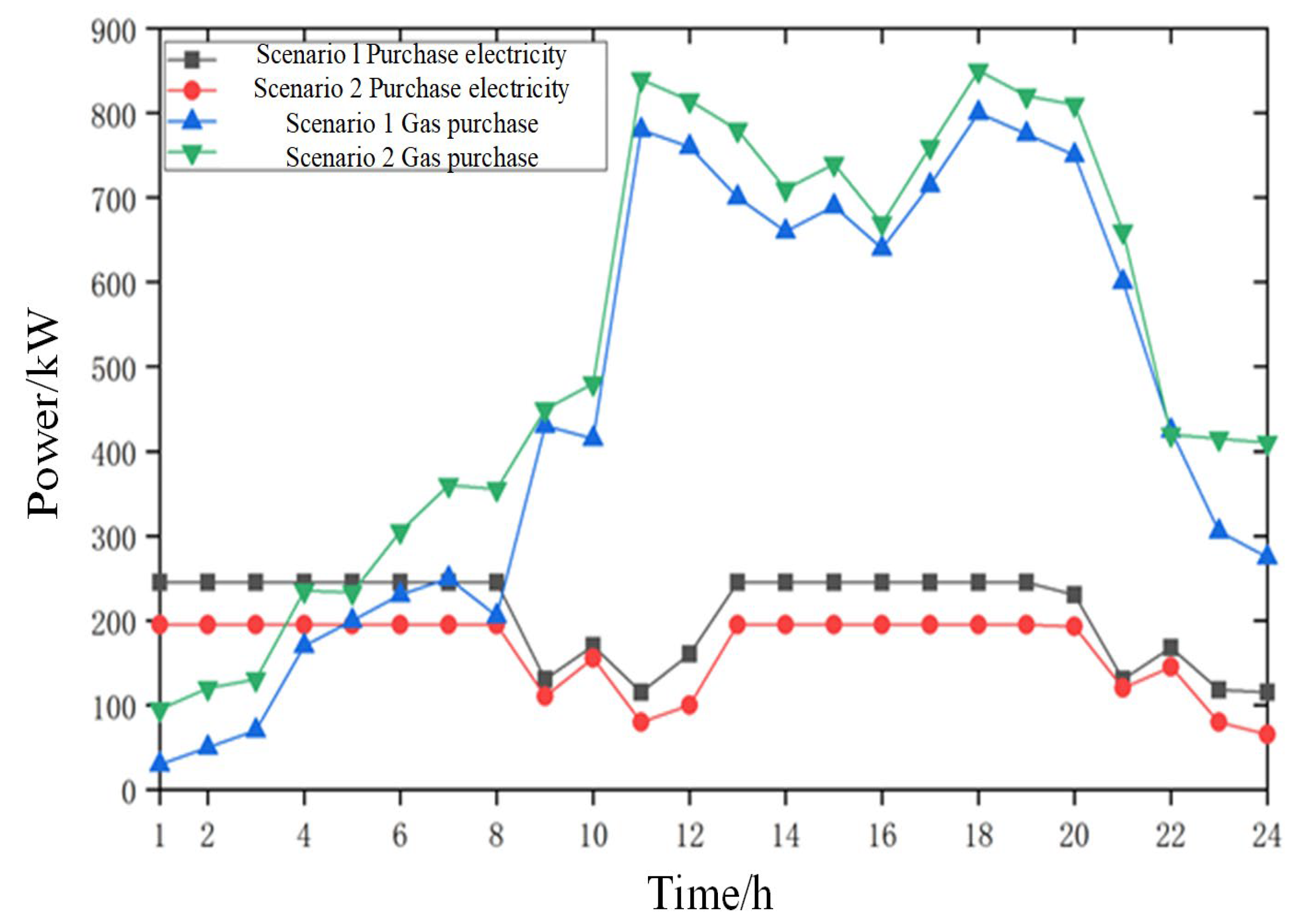
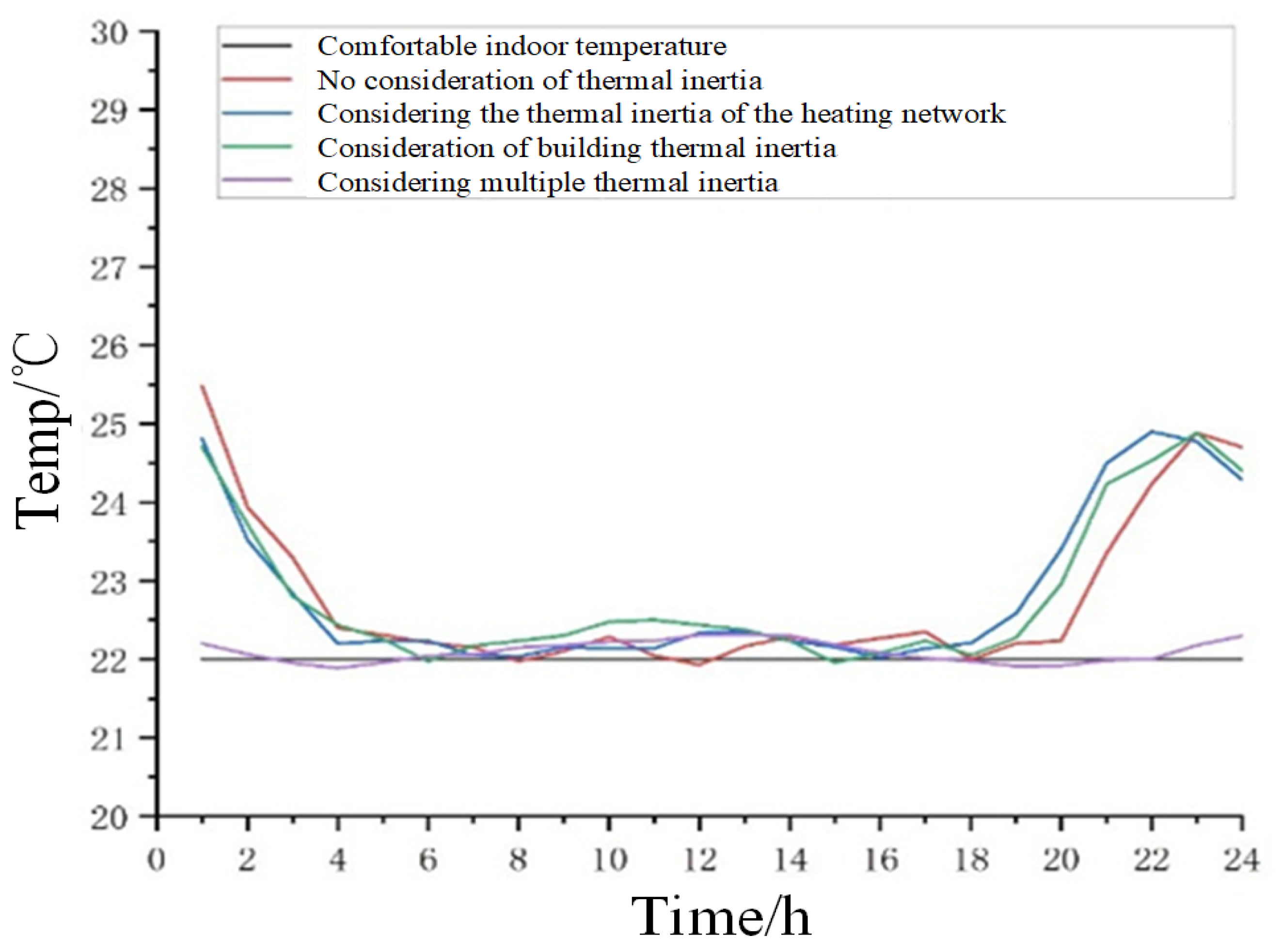
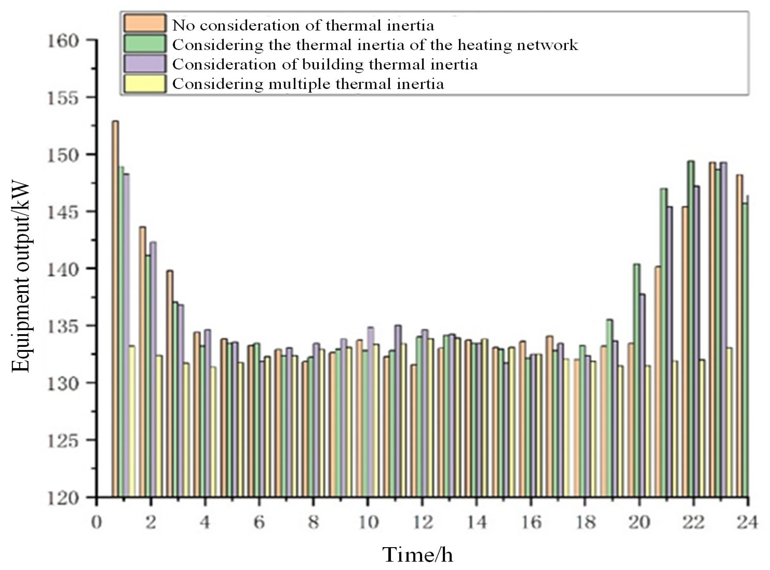
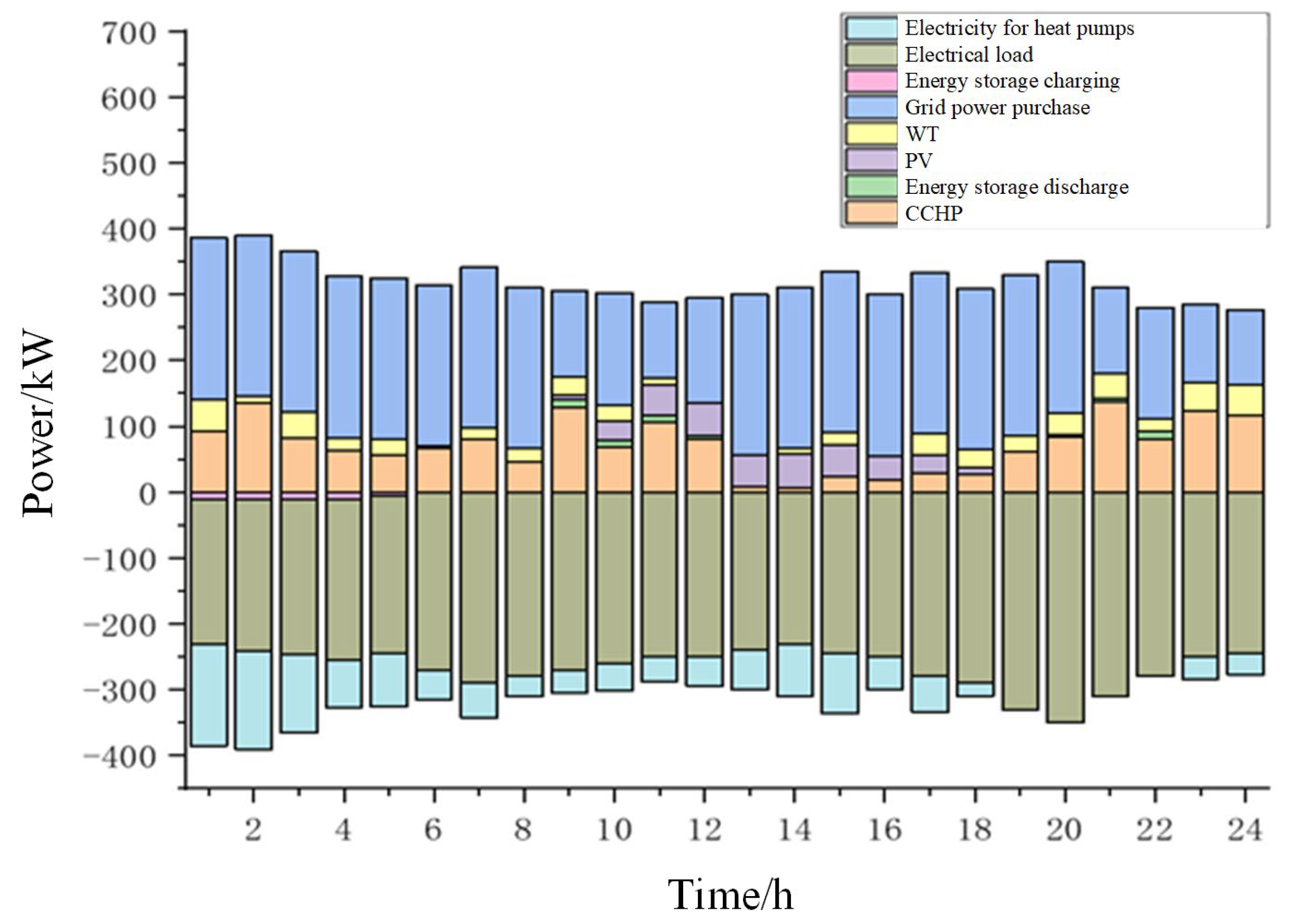
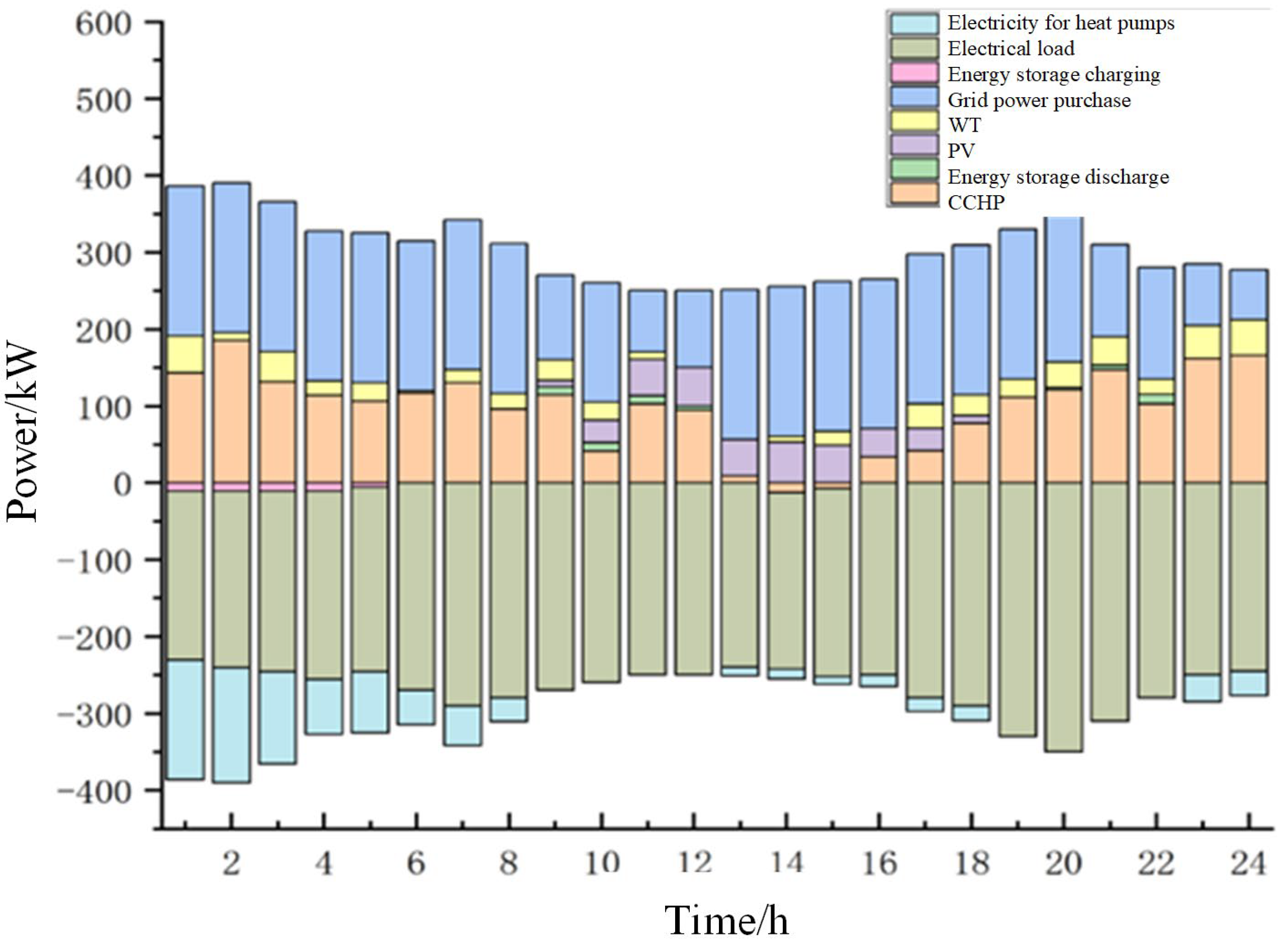
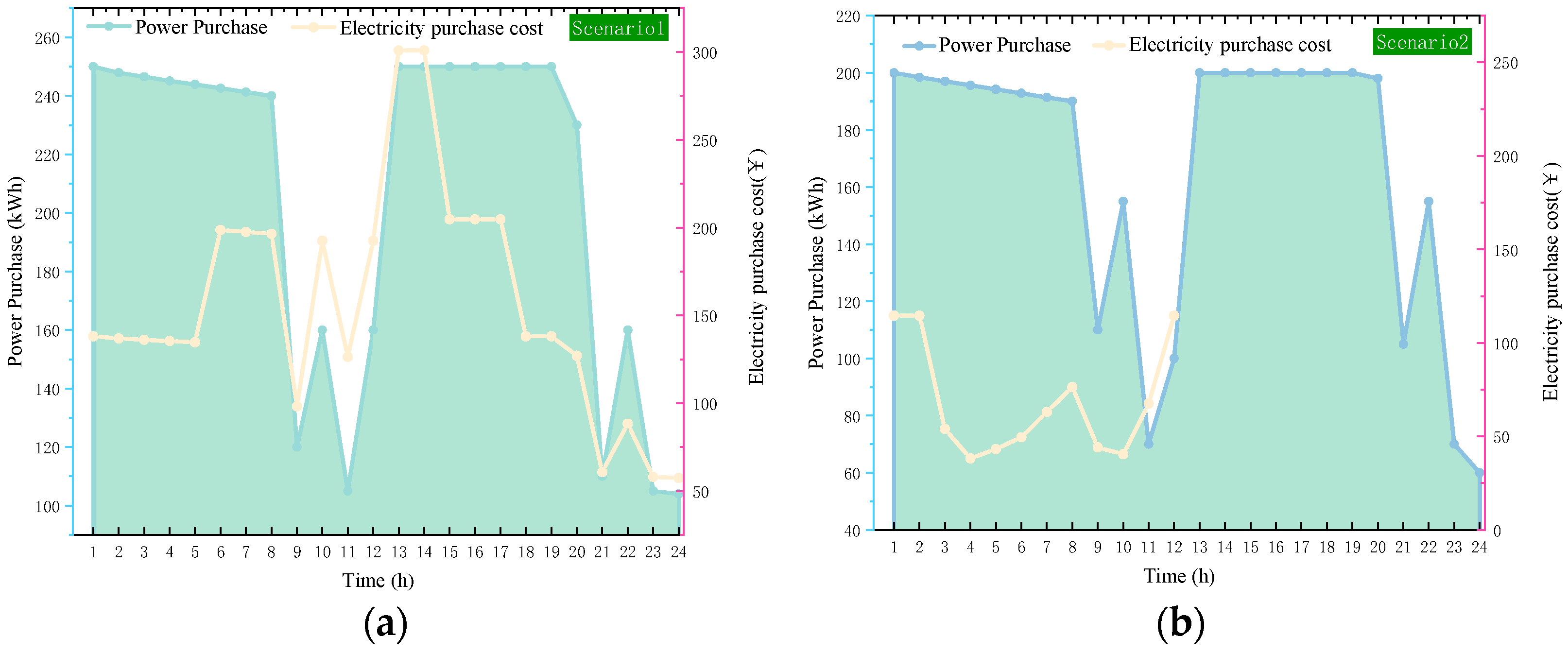
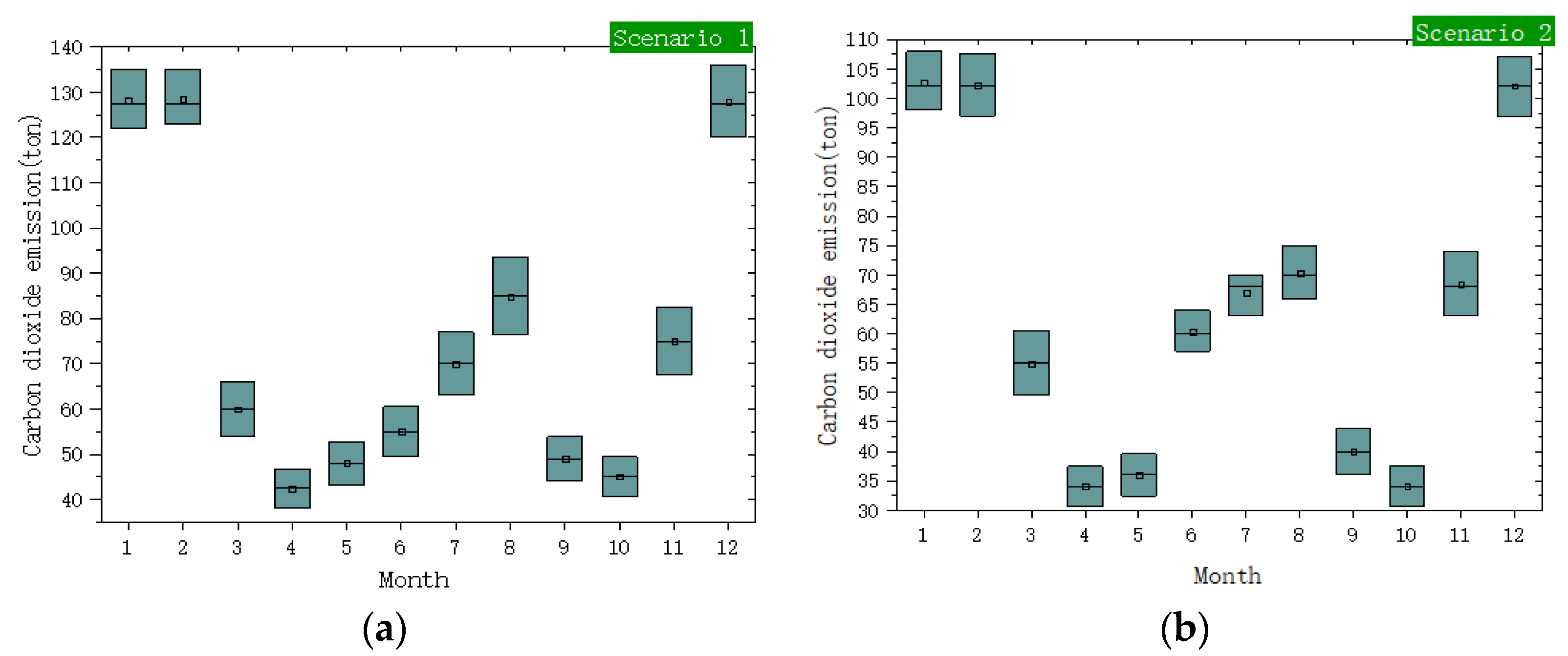
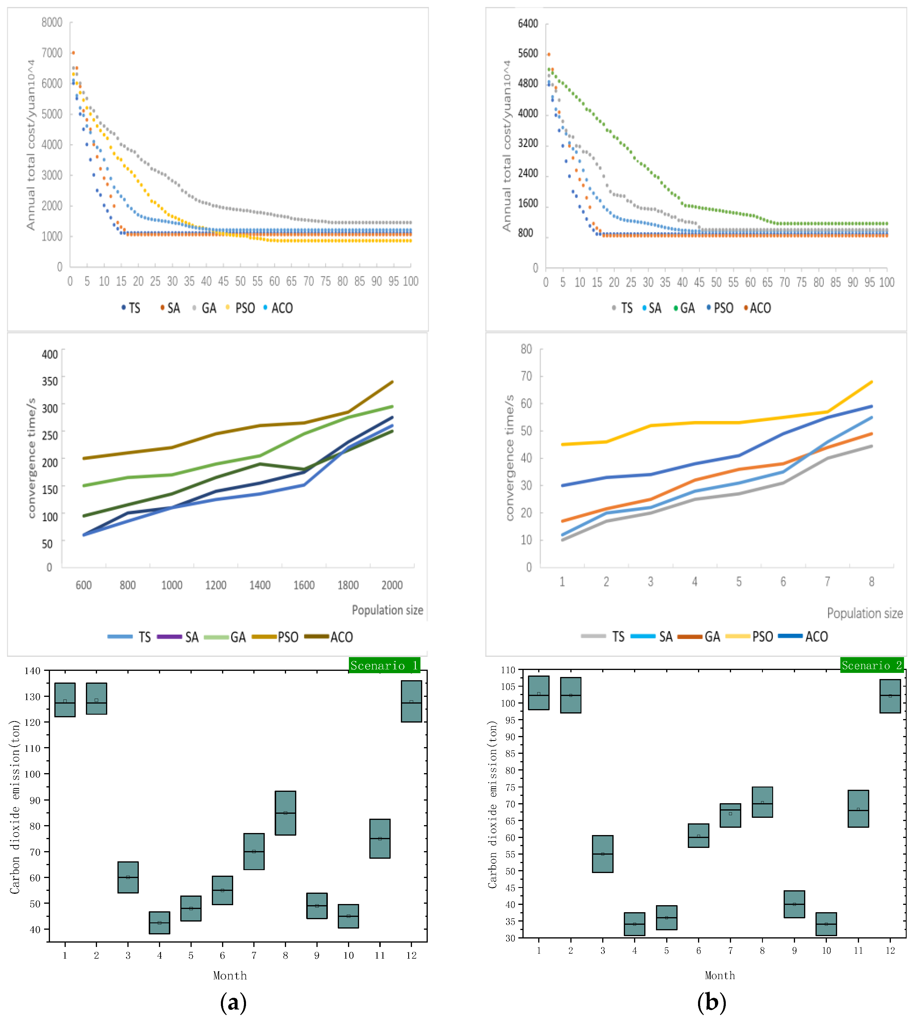
Disclaimer/Publisher’s Note: The statements, opinions and data contained in all publications are solely those of the individual author(s) and contributor(s) and not of MDPI and/or the editor(s). MDPI and/or the editor(s) disclaim responsibility for any injury to people or property resulting from any ideas, methods, instructions or products referred to in the content. |
© 2025 by the authors. Licensee MDPI, Basel, Switzerland. This article is an open access article distributed under the terms and conditions of the Creative Commons Attribution (CC BY) license (https://creativecommons.org/licenses/by/4.0/).