Electromechanical Model and Transient Behaviors of Power Systems

Abstract

A large-scale power system is often represented by a set of differential-algebraic equations, so-called electromechanical models. In this paper, it is shown that these models can have several analytical properties, which can be exploited to help the study of power system dynamics. These analytical properties, associated with the complete power system model and subsystem models, are described in detail. The implications of such analytical properties are also examined.

1. Introduction

The investigation of large-disturbance stability in power systems has a long history, spanning nearly a century. It is considered one of the core notions in the science of power system analysis. Utility engineers perform large-disturbance stability analysis on a routine basis. When performing operation studies, a utility engineer often comes up with four questions. Is the power system under study stable? Why is the system stable? How far away is the current system from being unstable? And how can one improve the stability margin of the system? The first question is usually answered using a computational approach, while the rest of the questions should be better addressed using an analytical approach.

Several methods are available in the literature, namely, the time-domain simulation method [1,2], direct methods [3], functional approximation methods [4], asymptotic expansion methods [5], etc. The focus of this work is not to look into the details of these methods; rather, the goal is to examine the analytical properties of power system models. It is assumed that the findings could be useful in developing new analytical methods and enhancing the understanding of power system dynamics.

While many methods have been developed to support the above-mentioned routine operations tasks, for the time being, the time-domain simulation method is the most widely accepted method in the industry. The drawback of the traditional time-domain simulation method is that it does not offer much insight into complex power system behavior. On the other hand, the topological configurations of power systems worldwide have become more and more complex in recent years. These two facts continue to remind us that there is a strong interest in developing analytical methods for stability analysis.

In large-disturbance stability studies, the power system under study is often represented by a set of nonlinear differential-algebraic equations, so-called electromechanical models. It was recently found by the authors that these models can be viewed as a nonlinear interconnected system which is composed of several subsystems that are functionally similar [6]. This decomposition–aggregation perspective allows one to better appreciate the analytical properties of power system models and opens up a new avenue for research. For instance, it was found in [6] that power flows during a transient are mainly affected by rotor subsystems, and the impact of the reactive power loop is less significant.

In fact, there are other means to accomplish model decomposition, for example, singular perturbation [7,8] and regular perturbation [9]. It was only in recent years that such analytical properties of power system models, profound in nature, began to attract attention. Many questions arise immediately: Do the subsystems obtained using a decomposition strategy have special properties? How do their properties relate to the overall transient behavior of power systems? Answers to the above questions are scattered in the literature; in this work, we consolidate some of the recent results into a single source.

While the focus of the present work is on the analytical aspects of power system transients, the fundamental significance of computational theory in power systems should not be underestimated. The power of the computational approach lies in its unique capacity to model complex system dynamics such as discontinuities, saturation, limits, etc. These are mathematical complications that are not easily treated using state-of-the-art analytical approaches. Therefore, the analytical and computational aspects of power system transients should be understood as the two building blocks of modern power system analysis; they are mutually indispensable.

The rest of this paper is organized as follows. Section 2 provides a taxonomy of the usual stability questions encountered in engineering studies, Section 3 examines the analytical properties of the complete model of power systems, Section 4 studies the analytical properties of the subsystems of power system models, and Section 5 concludes this study.

2. Stability Analysis Problems

Roughly speaking, the subject of power system transient analysis includes four building blocks, as summarized in Figure 1 below. It is well-known that an electromagnetic transient model precisely describes the physics of a power system, while an electromechanical model represents an approximation of the physics. In recent years, electromagnetic transient analysis has gained more and more attention due to the frequent occurrence of fast electromagnetic phenomena in systems with a high penetration of renewable energies [10]. Despite this, electromechanical transient analysis is still considered effective and efficient in the study of large-scale power system transients. In this work, we only focus on electromechanical transients.

As is well-known, power system electromechanical transients are governed by a set of differential-algebraic equations (DAEs), which can be written as follows [1]:

$$\left\{\begin{array}{l}\dot{x}=f(x,y,V), x(0)=x_0\\ g(x,y,V)=0\\ I(x,V)=YV\end{array}\right.$$

(1)

Here, $x$ denotes state variables such as rotor angles, etc.; y represents an auxiliary variable vector such as d-axis and q-axis currents; $V$ denotes network voltage phasors; $I(x,V)$ denotes current injections; and $Y$ denotes a network admittance matrix.

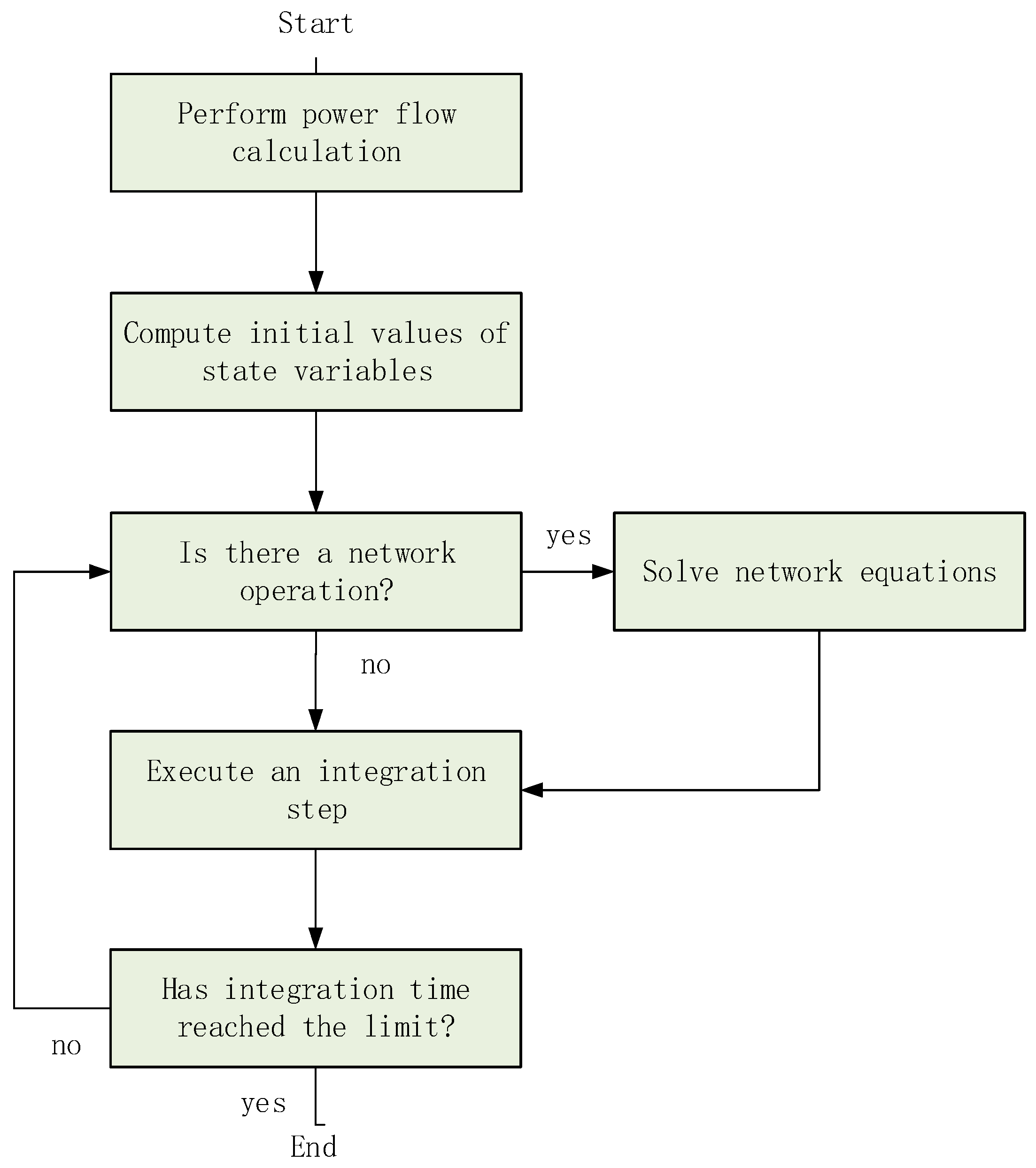
Efficient numerical methods are available for computing solutions to the above initial value problem, and the readers are referred to (for example) [1,2,11] for details. For convenience, Appendix A. provides a flowchart of the computational procedure. The main interest of this research is on the analytical aspects of the above system, a topic that received far less attention in the past.

The models and parameters of a power system under study can change, either intentionally or inevitably. Most often, utility engineers are interested in understanding voltage transient, as some parameters or models vary. As will become clear, transient analysis is largely concerned about how state vector x changes, as system parameters and models change. The model aspect of transient analysis includes four classes of questions, depending upon where the varying factors present.

A Class A question seeks to understand how a power system transient is affected as the parameters of controllers change. A familiar example is the investigation of the impact of the gains of fast excitation control. The model of such problems is stated as follows:

$$\left\{\begin{array}{l}\dot{\mathsf{\delta }}={\omega }_0(\mathsf{\omega }-1)\\ M\dot{\mathsf{\omega }}={\mathrm{P}}_M-{\mathrm{E}}_q^{\prime }{\mathrm{I}}_q-({\mathrm{X}}_q-{\mathrm{X}}_q^{\prime }){\mathrm{I}}_d{\mathrm{I}}_q\\ {\mathrm{T}}_{d0}^{\prime }{\dot{\mathrm{E}}}_q^{\prime }={\mathrm{E}}_{\mathrm{f}d}-{\mathrm{E}}_q^{\prime }-({\mathrm{X}}_d-{\mathrm{X}}_d^{\prime }){\mathrm{I}}_d\\ {\mathrm{T}}_{\mathrm{A}}{\dot{\mathrm{E}}}_{\mathrm{f}d}={\mathrm{K}}_{\mathrm{A}}({\mathrm{V}}_{\mathrm{ref}}-|{\mathrm{V}}_{\mathrm{G}}|)-{\mathrm{E}}_{\mathrm{f}d}\end{array}\right.$$

(2)

$$X_q\circ I_q+j(E_q^{\prime }-X_d^{\prime }\circ I_d)=e^{-j(\delta -\pi /2)}\circ V_G$$

(3)

$$\left\{\begin{array}{ll}\hfill Y_{\mathrm{GG}}{V}_{\mathrm{G}}+Y_{\mathrm{GL}}{V}_{\mathrm{L}}& =E_q^{\prime }\circ e^{j\mathsf{\delta }}./(j{X}_d^{\prime })\hfill \\ \hfill Y_{\mathrm{LG}}{V}_{\mathrm{G}}+Y_{\mathrm{LL}}{V}_{\mathrm{L}}& ={\overline{S}}_L./{\overline{V}}_L\hfill \end{array}\right.$$

(4)

When studying the problem, we assume that the gain vector ${\mathrm{K}}_{\mathrm{A}}$ takes different values, and understand that the power flow of the system remains constant, so mechanical powers ${\mathrm{P}}_M$ and generator voltage references ${\mathrm{V}}_{\mathrm{ref}}$ remain constant, and so are the initial values of $\mathsf{\delta }$, $\mathsf{\omega }$ and ${\mathrm{E}}_q^{\prime }$. In the above model, (3) represents the set of interface equations, while (4) represents the set of network equations.

A Class A problem appears to be simpler compared to Class B, C, and D problems to be described subsequently. However, some of the problems in Class A can still be extremely challenging, for example, the impact of control saturation on system transient [12,13].

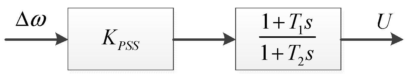
A Class B problem often reads as follows: what is the impact of commissioning/decommissioning a power system stabilizer? Figure 2 shows the control block diagram of a first-order power system stabilizer.

Formally, we are interested in knowing the impact of a power system stabilizer model on the overall performance of the system. The complete model of the system with a stabilizer is as follows, where the last set of equations represents the dynamics of stabilizers (interface and network equations are omitted):

$$\left\{\begin{array}{l}\dot{\mathsf{\delta }}={\omega }_0(\mathsf{\omega }-1)\\ M\dot{\mathsf{\omega }}={\mathrm{P}}_M-{\mathrm{E}}_q^{\prime }{\mathrm{I}}_q-({\mathrm{X}}_q-{\mathrm{X}}_d^{\prime }){\mathrm{I}}_d{\mathrm{I}}_q\\ {\mathrm{T}}_{d0}^{\prime }{\dot{\mathrm{E}}}_q^{\prime }={\mathrm{E}}_{\mathrm{f}d}-{\mathrm{E}}_q^{\prime }-({\mathrm{X}}_d-{\mathrm{X}}_d^{\prime }){\mathrm{I}}_d\\ {\mathrm{T}}_{\mathrm{A}}{\dot{\mathrm{E}}}_{\mathrm{f}d}={\mathrm{K}}_{\mathrm{A}}({\mathrm{V}}_{\mathrm{ref}}-|{\mathrm{V}}_{\mathrm{G}}|)-{\mathrm{E}}_{\mathrm{f}d}\\ {\dot{x}}_{PSS}=f_{PSS}(\delta ,\omega ,E_q^{\prime })\end{array}\right.$$

(5)

Obviously, including stabilizer models increases the order of the system model. This hints that a Class B problem is in general more difficult than a Class A problem. Here, we also understand that the power flow of the system remains constant.

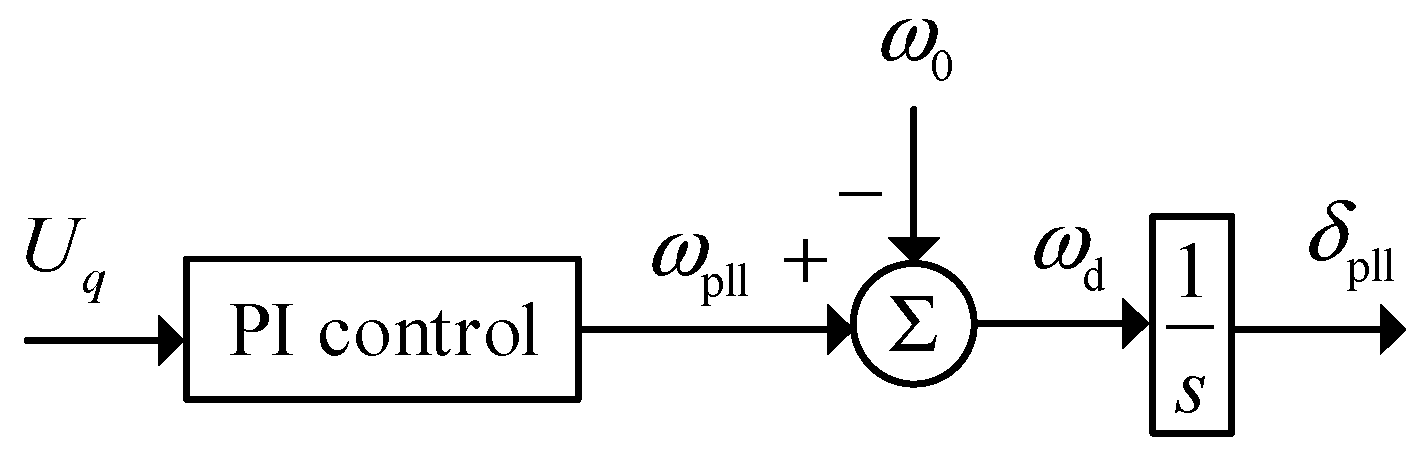
It is perhaps meaningful to give more examples of Class B problems. The first concerns a study on the impact of over-excitation limiters and on-line tap changers. They are not modeled in traditional simulations; however, in order to understand long-term voltage instability, they should be included in the simulation [14]. The second example concerns a study on phase-locked-loops (Figure 3 below), which have a significant impact on system performance at the 10 millisecond time-scale [15]; they are often not modeled in electromechanical transient studies.

A Class C problem asks how the continuous variations in operating conditions, such as mechanical power ${\mathrm{P}}_M$ and $V_{ref}$ profile, affect stability. The problem looks as follows (again, interface and network equations are omitted):

$$\left\{\begin{array}{l}\dot{\mathsf{\delta }}={\omega }_0(\mathsf{\omega }-1)\\ M\dot{\mathsf{\omega }}={\mathrm{P}}_M-{\mathrm{E}}_q^{\prime }\circ {\mathrm{I}}_q-({\mathrm{X}}_q-{\mathrm{X}}_d^{\prime }){\mathrm{I}}_d{\mathrm{I}}_q\\ {\mathrm{T}}_{d0}^{\prime }{\dot{\mathrm{E}}}_q^{\prime }={\mathrm{E}}_{\mathrm{f}d}-{\mathrm{E}}_q^{\prime }-({\mathrm{X}}_d-{\mathrm{X}}_d^{\prime }){\mathrm{I}}_d\\ {\mathrm{T}}_{\mathrm{A}}{\dot{\mathrm{E}}}_{\mathrm{f}d}={\mathrm{K}}_{\mathrm{A}}({\mathrm{V}}_{\mathrm{ref}}-|{\mathrm{V}}_{\mathrm{G}}|)-{\mathrm{E}}_{\mathrm{f}d}\end{array}\right.$$

(6)

Here, the order of the state space model of the power system does not change while power flow changes. This indicates that the initial values of the state variables δ, ω, and ${\mathit{E}}_q^{\prime }$ also change accordingly. An example of such problems, sometimes known as preventive control, concerns the study of the impact of increasing the power flow across a major transmission path. See reference [16] for some early efforts attempting to answer such questions. It is sometimes helpful to view the above problem from the perspective of optimization; see [17,18,19]. There are alternative parametric analysis methods in the literature; see reference [4] for a survey on the so-called polynomial approximation method.

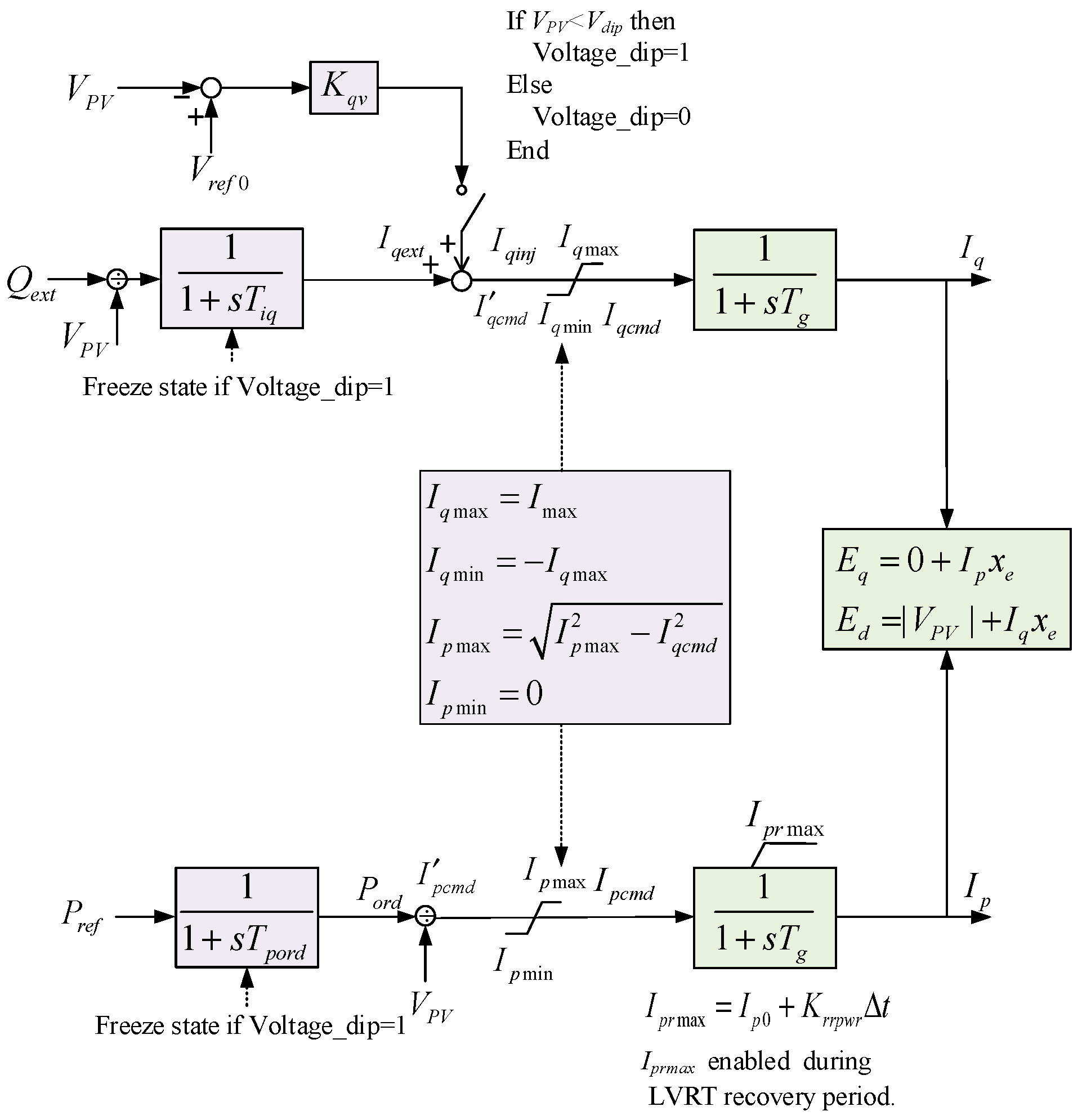
The Class D problems are most complicated. Here, one desires to investigate the impact of the connection/disconnection of important electrical elements (for example, a converter, see Figure 4) on system transients. Clearly, when addressing this class of questions, both the expressions and order of the system model can change, and so does the power flow.

In summary, a power system transient analysis can present a hierarchy of progressively difficult engineering questions [20]. Historically, Class A and Class B problems have attracted extensive and intensive research, while much less is known about Class C and Class D challenges.

3. Properties of the Complete System

This section reviews and studies the properties of the complete system model of power systems.

3.1. Multi-Stage Property

Figure 5 below shows the control block diagram of a somewhat simplified WECC photovoltaic generator model [21]. It should be noted that plant models are not included here, partly because plant controls are typically slower, and partly because we intend to build a simplified PV model. Lookup tables VDL1 and VDL2 are designed to allow for a maximum output of reactive current and to limit active current (usually being zero or half the nominal current); they are not included either.

To gain some flavor of the multi-stage property, let us suppose a photovoltaic generator is integrated to a system that experiences a fault electrically close to the photovoltaic generator terminal bus. The response of the generator usually involves three stages; see Figure 6 below. The figure demonstrates that the dynamics of a photovoltaic generator develops in three stages, namely, fault-on stage, recovery stages, and normal operation stage.

In the fault-on stage, the terminal voltage Vt is lower than the threshold Vdip. Here, Vdip is set to 0.9 pu. The Dynamic Voltage Support function is activated, and it injects extra reactive current Iqinj into the grid [22]. At this stage, the generator keeps outputting high reactive current and lower active current.

In the recovery stage, the terminal voltage Vt returns to normal value, and the active current recovers under ramp rate limit rrpwr [23]. Here, typically, rrpwr = 100%/s. The reactive current recovers immediately, and the Dynamic Voltage Support control is de-activated.

During normal operations, Vt > Vdip, so the generator assumes constant P-Q control, and the active and reactive controllers are modeled as 1/(1 + sTpord) and 1/(1 + sTiq), respectively.

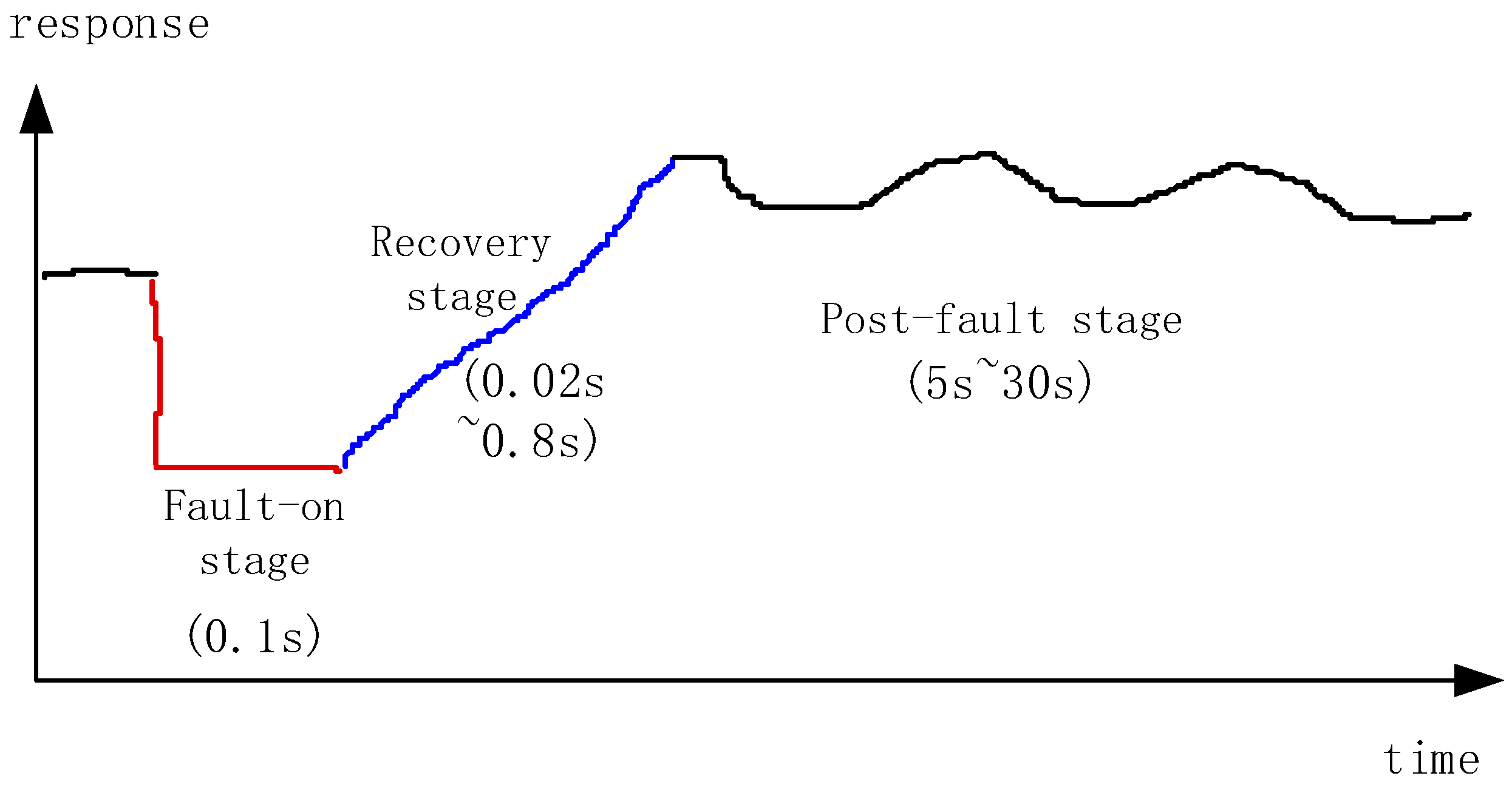
The response of the photovoltaic generators mentioned above is rather typical. When a power system under stable operation experiences a disturbance, such as three-phase-to-ground fault, it enters a period of transient, which typically develops in three stages, as Figure 7 shows. This is mainly dictated, as will become clear later, by the behaviors of renewable resources and HVDC systems.

In the fault-on stage, the fault persists and, after (say) 0.1 s, it becomes cleared. During this period, the voltage at the faulty substation drops to zero, and the voltage level in nearby substations is also very low. Because of the presence of a low-voltage profile, synchronous machines output extremely high currents, nevertheless remaining connected to the bulk of the system. Renewable energy units nearby should assume the so-called Low-Voltage-Ride-Through (LVRT) control logic, outputting typically higher reactive power currents and lower active power currents. During this stage, HVDC links can experience either commutation failures or blockings, depending on the distance between the faulty substation and HVDC converters. The system in fault-on stage can be represented as follows:

$$\left\{\begin{array}{l}\dot{x}=f_F(x,V), x(0)=x_0\\ g_F(x,V)=0\\ I(x,V)=Y_{F}V\end{array}\right.$$

(7)

In the recovery stage, usually the voltage profile of the system becomes normal. However, synchronous machines can not immediately return to stable operation; rather, they tend to swing against each other, introducing line flow oscillations. The swings of machines generally expand the second and the third stage. At this stage, renewable energy units can keep operating under the recovery control logic for less than some 0.8 s. HVDC links, operating under recovery control logic, take about 0.02 s to return back to stable operation. The model of the system during recovery stage is different from that of the fault-on stage, and it can be written as:

$$\left\{\begin{array}{l}\dot{x}=f_R(x,y,V), x(t_R)=x_R\\ g_R(x,y,V)=0\\ I_R(x,V)=Y_{R}V\end{array}\right.$$

(8)

The last stage expands a period of approximately 5~30 s. For a long-term voltage stability problem, not to be addressed in this text, this stage can last up to 5–10 min. During this transient period, synchronous machines slowly return to steady-state operation, while renewable energy units and HVDC links quickly stabilize and assume normal power control. Finally, the model of the system during the after-fault stage can be expressed as follows:

$$\left\{\begin{array}{l}\dot{x}=f_{PF}(x,y,V), x(t_{PF})=x_{PF}\\ g_{PF}(x,y,V)=0\\ I(x,V)=Y_{PF}V\end{array}\right.$$

(9)

Reference [3] offers a detailed account of the properties of multi-state behaviors of power systems.

3.2. DAE Properties

In the previous sub-section, it is seen that during each stage, the model of a power system is represented by a set of differential-algebraic equations. In this sub-section, we study the properties of such models.

The dynamics of a power system during each stage mentioned in previous sub-section can be re-written as follows:

$$\left\{\begin{array}{l}\dot{\mathrm{x}}=\mathrm{f}(\mathrm{x},\mathrm{y})\\ \mathbf{0}=\mathrm{g}(\mathrm{x},\mathrm{y})\end{array}\right.,$$

(10)

Let Jalg = ∂g/∂y be the Jacobian matrix of network equations g(x, y), and define the singular surface in state space, as follows:

$$S=\left\{(x,y)\left|\det J_{\mathrm{alg}}=0,g(x,y)=0\right.\right\}.$$

(11)

Then, the quasi-stability boundary $\partial \overline{A}$ of (10) can be stated as follows [24]:

$$\partial \overline{A}=\overline{\underset{i}{\cup }{W}^S(z_i)\underset{j}{\cup }(S\cap \partial \overline{A})},$$

(12)

where z_i denotes an unstable equilibrium point of (10), and W^S(z_i) is the corresponding stable manifold. Roughly speaking, the above fundamental result states that the degree of singularity of J_alg can be viewed as a short-term voltage stability margin.

To proceed, consider now an N-bus power network interconnected with m synchronous machines and n constant power injections. Let V be the network voltage vector, I be the current injection vector, and Y be the nodal admittance matrix. The set of network equations can be partitioned as follows:

$$\left[\begin{array}{cc}{\mathrm{Y}}_{\mathrm{GG}}& {\mathrm{Y}}_{\mathrm{GC}}\\ {\mathrm{Y}}_{\mathrm{CG}}& {\mathrm{Y}}_{\mathrm{CC}}\end{array}\right]\left[\begin{array}{c}{\mathrm{V}}_{\mathrm{G}}\\ {\mathrm{V}}_{\mathrm{C}}\end{array}\right]=\left[\begin{array}{l}{\mathrm{I}}_{\mathrm{G}}\\ {\mathrm{I}}_{\mathrm{C}}\end{array}\right],$$

(13)

where the subscripts G and C correspond to synchronous machine nodes and constant power nodes, respectively. Notice that current injections IG can be expressed as follows:

$${\mathrm{I}}_{\mathrm{G}}=-\mathrm{jdiag}{\left({\mathrm{X}}_d^{\prime }\right)}^{-1}\left({\mathrm{E}}^{\prime }-{\mathrm{V}}_{\mathrm{G}}\right),$$

(14)

where diag(∙) represents a diagonal matrix; ${\mathrm{V}}^{\ast }$ denotes the complex conjugate of V; ${\mathrm{X}}_d^{\prime }$ denotes the vector of d-axis transient reactance; and ${\mathrm{E}}^{\prime }=\left|{\mathrm{E}}^{\prime }\right|\circ e^{\mathrm{j}\mathsf{\delta }}$ is the vector of generator internal voltages, with the constant magnitudes $\left|{\mathrm{E}}^{\prime }\right|$ and the rotor angles δ. The current injections IC are calculated as follows:

$${\mathrm{I}}_{\mathrm{C}}=\mathrm{diag}{\left({\mathrm{V}}_{\mathrm{C}}^{\ast }\right)}^{-1}{\mathrm{S}}_{\mathrm{C}}^{\ast },$$

(15)

where SC = PC + jQC. Here, the negative entries in PC represent active power loads, and the positive entries represent constant power generations.

The Jacobian matrix of the above set of network equations can be computed as follows:

$${\mathrm{J}}_{\mathrm{alg}}=\left[\begin{array}{cc}{\displaystyle \frac{\partial {\mathrm{g}}_p}{\partial {\mathrm{V}}_x}}& {\displaystyle \frac{\partial {\mathrm{g}}_p}{\partial {\mathrm{V}}_y}}\\ {\displaystyle \frac{\partial {\mathrm{g}}_q}{\partial {\mathrm{V}}_x}}& {\displaystyle \frac{\partial {\mathrm{g}}_q}{\partial {\mathrm{V}}_y}}\end{array}\right],$$

(16)

where

$$\left\{\begin{array}{l}{\displaystyle \frac{\partial {\mathrm{g}}_p}{\partial {\mathrm{V}}_x}}=\mathrm{diag}{\mathrm{I}}_x+\mathrm{diag}\left({\mathrm{V}}_y\right){\mathrm{B}}^{\prime }+\mathrm{diag}\left({\mathrm{V}}_x\right){\mathrm{G}}^{\prime }\\ {\displaystyle \frac{\partial {\mathrm{g}}_p}{\partial {\mathrm{V}}_y}}=\mathrm{diag}{\mathrm{I}}_y-\mathrm{diag}\left({\mathrm{V}}_x\right){\mathrm{B}}^{\prime }+\mathrm{diag}\left({\mathrm{V}}_y\right){\mathrm{G}}^{\prime }\\ {\displaystyle \frac{\partial {\mathrm{g}}_q}{\partial {\mathrm{V}}_x}}=-\mathrm{diag}{\mathrm{I}}_y-\mathrm{diag}\left({\mathrm{V}}_x\right){\mathrm{B}}^{\prime }+\mathrm{diag}\left({\mathrm{V}}_y\right){\mathrm{G}}^{\prime }\\ {\displaystyle \frac{\partial {\mathrm{g}}_q}{\partial {\mathrm{V}}_y}}=\mathrm{diag}{\mathrm{I}}_x-\mathrm{diag}\left({\mathrm{V}}_y\right){\mathrm{B}}^{\prime }-\mathrm{diag}\left({\mathrm{V}}_x\right){\mathrm{G}}^{\prime }\end{array}\right..$$

(17)

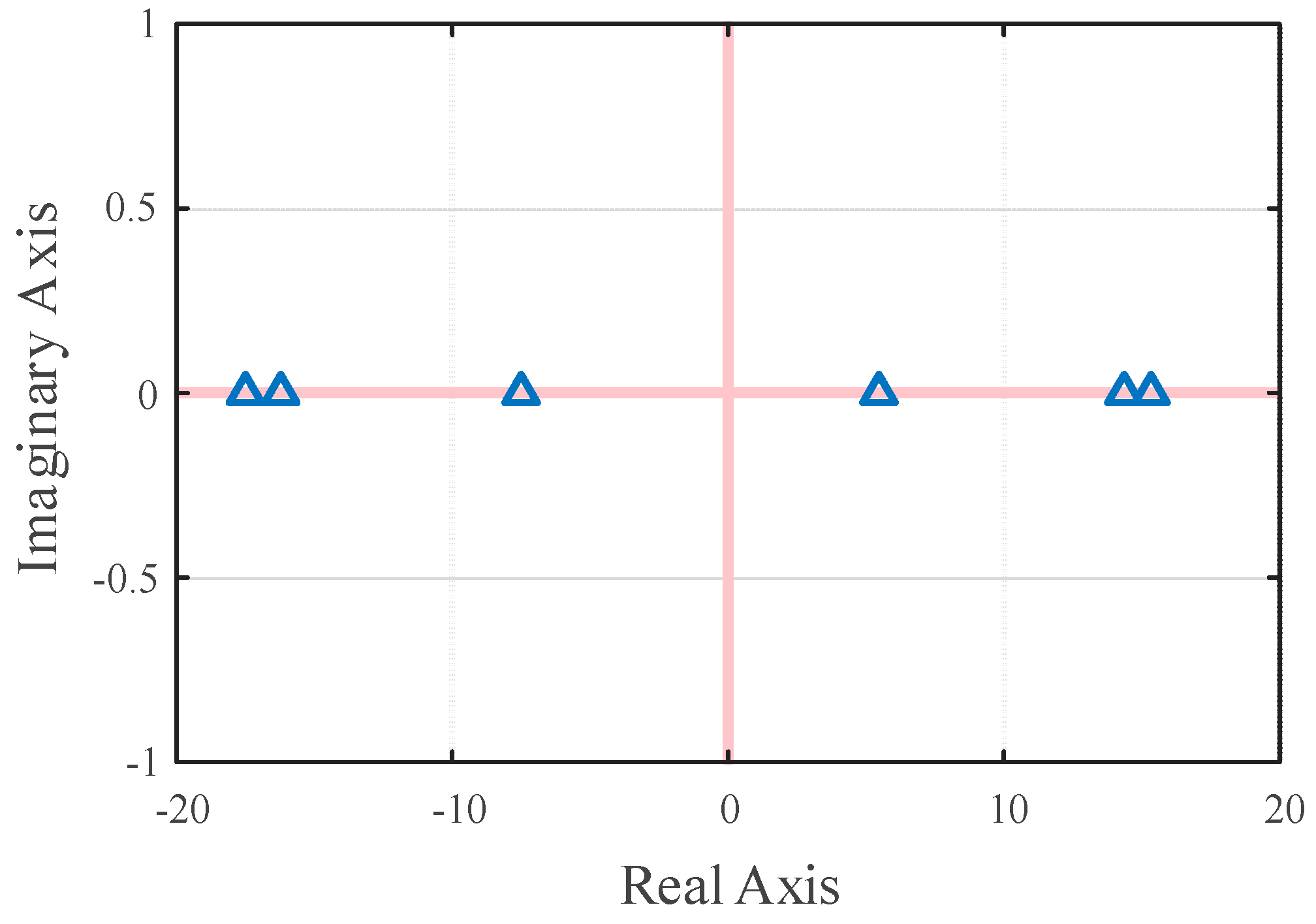
It is interesting to observe that since Ix and Iy are significantly smaller than the diagonal entries of B′, as a result, Jalg often has an equal amount of positive and negative eigenvalues (see Figure 8).

The property of the Jacobian matrix described above makes it very convenient when assessing voltage stability margins. Readers are referred to [25] for details.

3.3. Two Time-Scale Property

First, we briefly review the theory of singular perturbation [26]. Consider the following two time-scale system:

$$\begin{array}{l}\dot{x}=f(x,z), x(0)=x_0\\ \epsilon \dot{z}=g(x,z), z(0)=z_0\end{array}$$

(18)

where ε is a small positive parameter and $\epsilon <<1$. Here, $x\in {ℝ}^n$ denotes the set of slow variables and $z\in {ℝ}^m$ denotes fast variables.

The reduced system corresponding to (18) is represented as follows:

$$\begin{array}{l}\dot{x}=f(x,z), x(0)=x_0\\ 0=g(x,z)\end{array}$$

(19)

For convenience, let us take $(\underset{\_}{x}(t),\underset{\_}{z}(t))$ as the solution of the above system.

Let $\widehat{z}=z-\underset{\_}{z}$, performing a transformation $\tau =t/\epsilon$, and let $\epsilon =0$. We obtain the so-called boundary layer system:

$${\displaystyle \frac{d\widehat{z}}{d\tau }}=g({\underset{\_}{x}}_0,{\underset{\_}{z}}_0+\widehat{z}), \widehat{z}(0)=z_0-{\underset{\_}{z}}_0$$

(20)

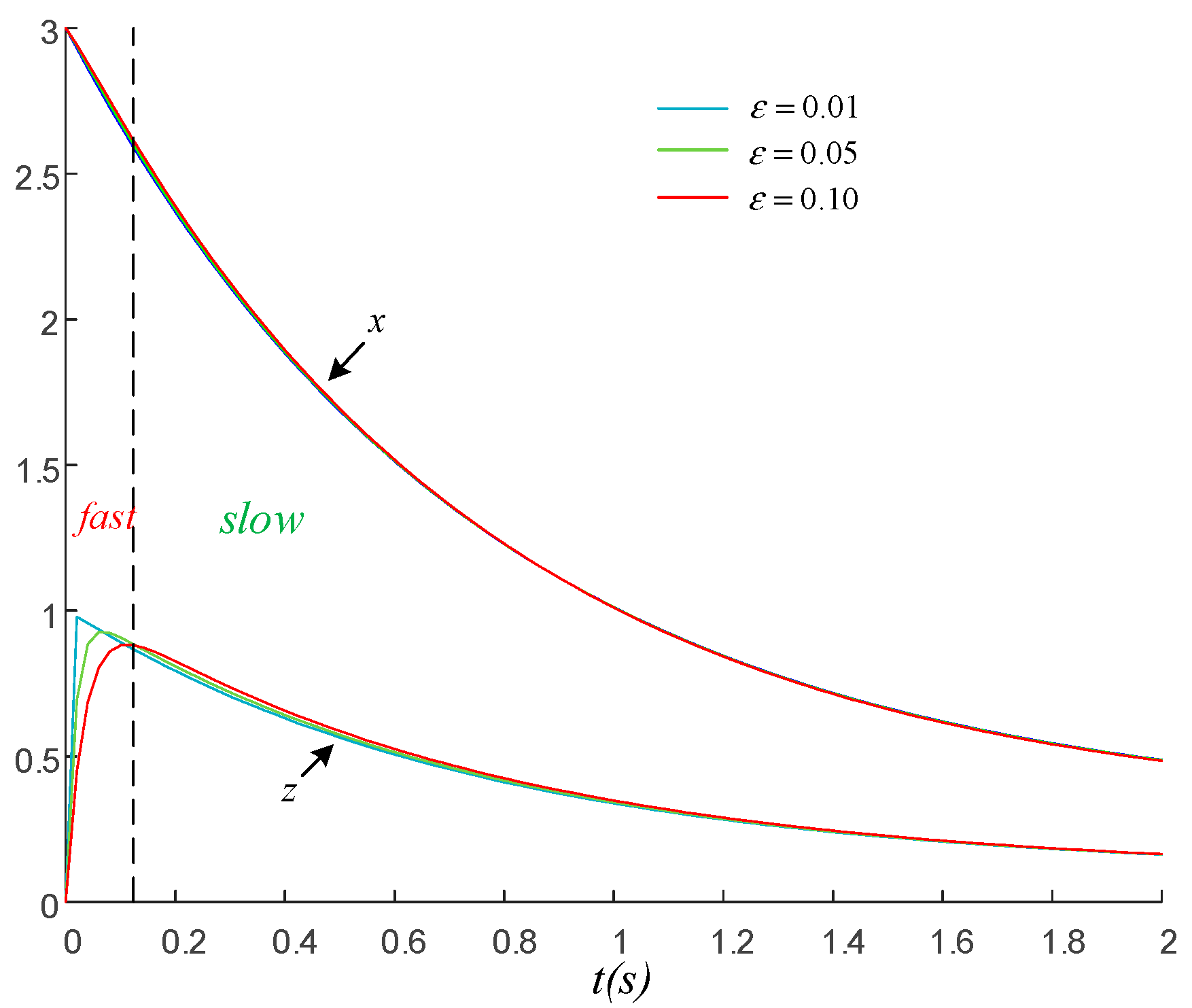
A fundament result of singular perturbation theory states that, under mild conditions, for $t\in [0,T]$, there is

$$\begin{array}{l}x(t)=\underset{\_}{x}(t)+o(\epsilon )\\ z(t)=\underset{\_}{z}(t)+\widehat{z}(t/\epsilon )+o(\epsilon )\end{array}$$

(21)

Figure 9 shows the curves of x(t) and z(t) when parameter ε takes different values.

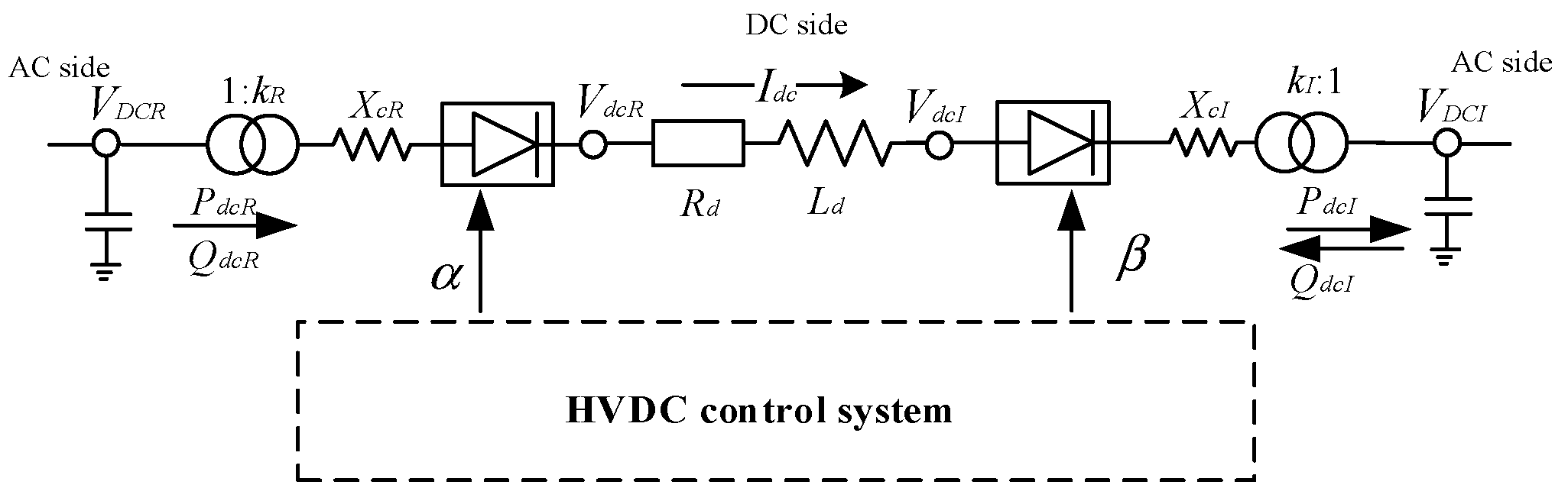
Now, let us proceed to show the application of the above theory to over-voltage analysis in power systems. Figure 10 shows the diagram of a HVDC tie. The notations adopted in the diagram are standard, and the readers are referred to (say) [27] for reference. The simulation results described in the section were obtained using a Matlab code written by the authors.

The electro-mechanical model of a HVDC tie is as follows:

$$\begin{array}{l}{V}_{dcR}=k_R{V}_{DCR}\cos \alpha -X_{cR}{I}_{dc}, V_{dcI}=k_I{V}_{DCI}\cos \beta +X_{cI}{I}_{dc}\\ P_{dcR}=V_{dcR}{I}_{dc}, \hspace{1em}\hspace{1em}\hspace{1em}\hspace{1em}\hspace{1em} P_{dcI}=V_{dcI}{I}_{dc}\\ \cos {\phi }_R=V_{dcR}/(k_R{V}_{DCR}),\hspace{1em}\hspace{1em}\cos {\phi }_I=V_{dcI}/(k_I{V}_{DCI})\\ Q_{dcR}=P_{dcR}\tan {\phi }_R,\hspace{1em}\hspace{1em}\hspace{1em}\hspace{1em} Q_{dcI}=P_{dcI}\tan {\phi }_I\end{array}$$

(22)

The transmission line is represented by the following:

$$L_d{\dot{I}}_{dc}=V_{dcR}-V_{dcI}-R_d{I}_{dc}$$

(23)

It is appropriate to assume that the inverter dynamics of the second HVDC tie is not significantly affected after the blocking of the first HVDC tie. Hence, the state equations of the HVDC system are obtained as follows:

$$\begin{array}{l}{T}_{vp}{\dot{V}}_{dcRmes}=V_{dcR}-V_{dcRmes}\\ T_{Idcmes}{\dot{I}}_{dcmes}=I_{dc}-I_{dcmes}\\ T_{IdR}{\dot{x}}_1=P_{ref}/V_{dcRmes}-I_{dcmes}\\ \alpha =\pi -x_1-k_{IdR}(P_{ref}/V_{dcRmes}-I_{dcmes})\end{array}$$

(24)

In subsequent analysis, synchronous machines are represented by a third-order transient model with a first-order excitation system, as follows:

$$\begin{array}{l}\dot{\delta }={\omega }_0(\omega -1)\\ 2H\dot{\omega }=P_M-E_q^{\prime }{i}_q-D(\omega -1)\\ T_{do}^{\prime }{\dot{E}}_q^{\prime }=E_{fd}-E_q^{\prime }-(X_d-X_d^{\prime })i_d\\ T_A{\dot{E}}_{fd}=-E_{fd}+K_A(V_{ref}-\left|V_G\right|) \end{array}$$

(25)

where $V_G$ is the complex terminal voltage. In addition, we have the following:

$$\begin{array}{l}{i}_d+j{i}_q=I_G{e}^{j(\pi /2-\delta )}, \\ I_G=-j(E_q^{\prime }{e}^{j\delta }-V_G)/X_d^{\prime }\end{array}$$

(26)

Loads are modelled as complex constant powers, and they are denoted by vector $S_L$, with ${\overline{S}}_L$ being its conjugate. The set of network equations are as follows:

$$\left[\begin{array}{ccc}{Y}_{GG}& Y_{GDC}& Y_{GL}\\ Y_{DCG}& Y_{DC}& Y_{DCL}\\ Y_{LG}& Y_{LDC}& Y_{LL}\end{array}\right]\left[\begin{array}{c}{V}_G\\ V_{DC}\\ V_L\end{array}\right]=\left[\begin{array}{c}-j{E}_q^{\prime }\circ e^{j\delta }./X_d^{\prime }\\ \begin{array}{l}{\overline{S}}_{DC}./{\overline{V}}_{DC}\\ {\overline{S}}_L./{\overline{V}}_L\end{array}\end{array}\right]$$

(27)

where $V_{\mathrm{DC}}$ denotes the AC bus voltage of converters, $S_{DC}$ denotes the apparent power injection of converters, and $V_{\mathrm{L}}$ denotes the bus voltage vector.

For convenience, let $S_D^T=[S_{DC}^T S_L^T]$; likewise, we have $V_D^T=[V_{DC}^T V_L^T]$. Now, the set of network equations is re-formulated as follows:

$$\left[\begin{array}{cc}{Y}_{GG}& Y_{GD}\\ Y_{DG}& Y_{DD}\end{array}\right]\left[\begin{array}{c}{V}_G\\ V_D\end{array}\right]=\left[\begin{array}{c}-j{E}_q^{\prime }\circ e^{j\delta }./X_d^{\prime }\\ {\overline{S}}_D./{\overline{V}}_D\end{array}\right]$$

(28)

The key to simplifying HVDC analysis during over-voltage stages is that the typical time constants of the system models (22)–(25) differentiate in order of magnitude:

$$\left\{T_A,T_{Idcmes},T_{IdR},L_d\right\}<<\left\{H,T_{d0}^{\prime },T_{vp}\right\}$$

(29)

This suggests the following:

$$x={[{\delta }^T,{\omega }^T,{E^{\prime }}_q^T,V_{dcRmes}^T]}^T, z={[I_{dc}^T,I_{dcmes}^T,x_1^T,E_f^T]}^T$$

Apparently, the slow subsystem mostly includes the variables of synchronous machines, while the fast subsystem mainly includes the variables of HVDC current control. According to the standard theory of singular perturbation [26], the HVDC tie model reduces to:

$$\begin{array}{l}{V}_{dcR}-V_{dcI}-R_d{I}_{dc}=0,\\ I_{dc}-I_{dcmes}=0,\\ P_{ref}/V_{dcRmes}-I_{dcmes}=0,\\ T_{vp}{\dot{V}}_{dcRmes}=V_{dcR}-V_{dcRmes}\end{array}$$

(30)

From the first equation above, one has $V_{dcR}=V_{dcI}+R_d{I}_{dc}$, using the converter relationship $V_{dcI}=k_I{V}_{DCI}\cos \beta +X_{cI}{I}_{dc}$ from Equation (31), we obtain:

$$T_{vp}{\dot{V}}_{dcRmes}=k_I{V}_{DCI}\cos \beta +(R_d+X_{cI}){\displaystyle \frac{P_{ref}}{V_{dcRmes}}}-V_{dcRmes}$$

(31)

It is interesting to observe that the above equation is completely decoupled. Since $k_I{V}_{DCI}\cos \beta$ is assumed to be constant, thus the blocking of HVDC tie does not affect the solution of the equation. Let $V_{dcRmes0}$ be the solution obtained from power flow, we have:

$$V_{dcRmes}(t)=V_{dcRmes0}$$

(32)

This immediately suggests: $V_{dcR}$ and $I_{dc}$, thus $P_{d\mathrm{c}R}=V_{dcR}{I}_{dc}$, remain constant on the slow system trajectory. In addition, the reactive power consumption of a rectifier can be treated as a voltage-dependent reactive load.

In summary, the original fourth order HVDC model is simplified as the following static load:

$$\begin{array}{l}{P}_{d\mathrm{c}R}=V_{dcR0}{I}_{dc0}=P_{d\mathrm{c}R0}, \\ Q_{dcR}=I_{dc0}\sqrt{{(k_R\left|V_{DCR}\right|)}^2-V_{dcR0}^2}\end{array}$$

(33)

In the excitation model presented in (25), let $T_A=0$, one obtains $E_{fd}=K_A(V_{ref}-\left|V_G\right|)=0$, this suggests that the AC system can be reduced to:

$$\begin{array}{l}\dot{\delta }={\omega }_0(\omega -1)\\ 2H\circ \dot{\omega }=P_M-E_q^{\prime }{i}_q-D(\omega -1)\\ T_{do}^{\prime }\circ {\dot{E}}_q^{\prime }=K_A\circ (V_{ref}-\left|V_G\right|)-E_q^{\prime }-(X_d-X_d^{\prime })\circ i_d\end{array}$$

(34)

Equation (34), together with the algebraic Equations (28) and (33) constitute a reduced-order model for the original systems. Compared with the original model, the above model is much simpler and behave very much like a linear system, so it is not difficult to obtain analytical solutions for it, see [7] for details.

To end this section, it is noted that there are several other forms of two time-scale properties in power systems models, they can be equally useful. Because of space limitation, they are not covered in this work.

3.4. Weakly Nonlinear Property

The classic model of power systems can be expressed as:

$$\left\{\begin{array}{l}{\dot{\delta }}_i={\omega }_0{\omega }_i\\ M_i{\dot{\omega }}_i=P_{Oi}-{\displaystyle \sum _1^n{a}_{ij}\sin ({\delta }_{ij}-{\alpha }_{ij})}-D_i{\omega }_i\end{array}\right.,$$

(35)

where i = 1, …, n, n denotes the number of generators, P_O denotes the mechanical power of synchronous machines or active power reference value of renewable energy units, and:

$$a_{ij}=\left|E_i{E}_j{Y}_{ij}\right|, {\alpha }_{ij}=\arctan (B_{ij}/G_{ij})-\pi /2,$$

(36)

where E denotes the potential after the transient reactance of the synchronous machine or the internal voltage of the converter, Y denotes the Kron-reduced admittance matrix, G and B denote the real and imaginary parts of Y.

Consider now a nonlinear system:

$$\dot{x}=f(t,x,\epsilon ), x(t_0)=\eta (\epsilon ),$$

(37)

where f is sufficiently smooth in its arguments over a domain D. The utility of the perturbation methods is to exploit the smallness of the perturbation parameter $\epsilon$ to construct approximate solutions.

To apply the method, notice that:

$$\sin x=x-x^3/6+o(x^3).$$

(38)

Neglecting the higher order terms in (38) and considering 1/6 as a small parameter $\epsilon$, then Equation (35) is equivalent to:

$$\left\{\begin{array}{l}{\dot{\delta }}_i={\omega }_0{\omega }_i\\ M_i{\dot{\omega }}_i=P_{Oi}-{\displaystyle \sum _1^n{a}_{ij}({\delta }_{ij}-{\alpha }_{ij}-\epsilon {({\delta }_{ij}-{\alpha }_{ij})}^3)}-D_i{\omega }_i\end{array}\right..$$

(39)

Moving the equilibrium point to the origin, the above system is simplified as:

$$\left\{\begin{array}{l}{\dot{y}}_i={\omega }_0{\omega }_i\\ {\dot{\omega }}_i={\displaystyle \frac{P_{Oi}}{M_i}}-{\displaystyle \frac{1}{M_i}}{\displaystyle \sum _1^n{a}_{ij}(y_{ij}+{\varsigma }_{ij}-\epsilon {(y_{ij}+{\varsigma }_{ij})}^3)}-{\displaystyle \frac{D_i}{M_i}}{\omega }_i\end{array}\right.$$

(40)

where

$$y_i={\delta }_i-{\overline{\delta }}_i, {\varsigma }_{ij}={\overline{\delta }}_{ij}-{\alpha }_{ij},$$

(41)

And ${\overline{\delta }}_i$ denotes the equilibrium point. Simplifying the expansion of the above formula to get:

$$\begin{array}{l}{\dot{y}}_i={\omega }_0{\omega }_i\\ {\dot{\omega }}_i={\displaystyle \frac{P_{Oi}}{M_i}}-{\displaystyle \frac{1}{M_i}}{\displaystyle \sum _1^n{a}_{ij}({\varsigma }_{ij}-\epsilon {\varsigma }_{ij}^3)}-{\displaystyle \frac{1}{M_i}}{\displaystyle \sum _1^n{a}_{1,ij}{y}_{ij}}\\ \hspace{1em} +{\displaystyle \frac{\epsilon }{M_i}}\left({\displaystyle \sum _1^n{a}_{2,ij}{y}_{ij}^2}+{\displaystyle \sum _1^n{a}_{3,ij}{y}_{ij}^3}\right)\\ =P_{Oeqi}-{\displaystyle \frac{1}{M_i}}{\displaystyle \sum _1^n{a}_{1,ij}{y}_{ij}}+{\displaystyle \frac{\epsilon }{M_i}}{\displaystyle \sum _{k=2}^3\left({\displaystyle \sum _{j=1}^n{a}_{k,ij}{y}_{ij}^k}\right)}\end{array}$$

(42)

where

$$a_{1,ij}=a_{ij}-0.5a_{ij}{\varsigma }_{ij}^2, a_{2,ij}=3a_{ij}{\varsigma }_{ij}, a_{3,ij}=a_{ij}.$$

(43)

Assuming POeqi = 0, (42) can be re-written in the matrix form as:

$$\begin{array}{l}\left\{\begin{array}{l}\dot{y}={\omega }_0\omega \\ \dot{\omega }=A_{1}y+\epsilon F(y),\end{array}\right.\\ \Rightarrow \dot{x}=Ax+\epsilon F(x)\end{array}$$

(44)

where A1 and A denote the linear part, F denotes the nonlinear part. Introducing a linear transformation x = Uz, we get:

$$\dot{z}=U^{-1}AUz+\epsilon U^{-1}F(z)=\Lambda z+\epsilon U^{-1}F(z),$$

(45)

where U and Λ denote the right eigenvector matrix and the diagonal matrix formed by the eigenvalues of the A. Let the solution of (45) have the following asymptotic expansion:

$$z=z^0+\epsilon z^1+H.O.T..$$

(46)

where H.O.T. stands for higher order terms.

Substituting (46) into (45), and comparing the coefficients of on both sides of the equation, one obtains:

$$\left\{\begin{array}{l}{\dot{z}}^0=\Lambda z^0\\ {\dot{z}}^1=\Lambda z^1+U^{-1}F(z^0)\end{array}\right..$$

(47)

The above system can be solved based on the method of variation of constant as:

$$\begin{array}{l}{z}^0(t)=e^{\Lambda t}{U}_0\\ z^1(t)=e^{\Lambda t}{V}_0+e^{\Lambda t}{\displaystyle {\int }_{t_0}^t{e}^{-\Lambda s}{V}^{-1}F(e^{\Lambda s}{U}_0)ds\prime }\end{array}$$

(48)

where U0 and V0 denote constant vectors. Hence, the first-order approximation of the solution of the initial value problem (45) can be obtained as:

$$\begin{array}{l}z(t)=z^0(t)+\epsilon z^1(t)=\\ e^{\Lambda t}(U_0+\epsilon V_0+\epsilon {\displaystyle {\int }_{t_0}^t{e}^{\Lambda s}{U}^{-1}F(e^{-\Lambda s}{U}_0)ds})\end{array}.$$

(49)

The solution of the original system is therefore obtained as:

$$x(t)=x^0(t)+\epsilon x^1(t)=U{z}^0(t)+\epsilon U{z}^1(t).$$

(50)

It can be seen from (50) that the solution of the system is equal to the superposition of the linear part and the nonlinear part. When the independent variable of the sine function, that is, the power angle of each generator set does not swing a significantly, the linear solution can describe the dynamic motion of the system accurately. Quite often the disconnection of generator output or load does not have a great impact on the generator power angles, so that the linear model can be used for frequency stability analysis [9]. Furthermore, if the system trajectory is stable, it is still possible to obtain approximate solution using Equation (50).

3.5. Interconnection Property

In this sub-section we review a decomposition-aggregation strategy that was discovered recently by the authors [6]. The notion of decomposition-aggregation had been proposed in (say) [28,29,30,31], the goal was to reduce computational effort. This traditional strategy proceeds by dividing a large-scale system into smaller control areas. This is not the subject of this research. In our work [6], we revisited this divide-and-conquer paradigm, presenting a very different implementation strategy: decomposing the original system model based on the dynamic character of the subsystems. It is found that this new strategy allows one to look into the analytical properties of a power system model from a new perspective.

To proceed, let the synchronous machines assume the well-known one-axis model and the exciter assume a first-order model, the complete model of the system are expressed as (see reference [1] for the derivation of this well-known model):

$$\left\{\begin{array}{cc}\hfill \dot{\mathsf{\delta }}& ={\omega }_0(\mathsf{\omega }-1)\hfill \\ \hfill \hspace{1em}2\mathrm{H}\dot{\mathsf{\omega }}& ={\mathrm{P}}_{\mathrm{m}}-{\mathrm{I}}_q\circ {\mathrm{E}}_q^{\prime }-({\mathrm{X}}_q^{\prime }-{\mathrm{X}}_d^{\prime })({\mathrm{I}}_d{\mathrm{I}}_q)\hfill \\ \hfill {\mathrm{T}}_{d0}^{\prime }{\dot{\mathrm{E}}}_q^{\prime }& ={\mathrm{E}}_{\mathrm{f}d}-{\mathrm{E}}_q^{\prime }-({\mathrm{X}}_d-{\mathrm{X}}_d^{\prime }){\mathrm{I}}_d\hfill \\ \hfill {\mathrm{T}}_{\mathrm{A}}{\dot{\mathrm{E}}}_{\mathrm{f}d}& ={\mathrm{K}}_{\mathrm{A}}({\mathrm{V}}_{\mathrm{ref}}-|{\mathrm{V}}_{\mathrm{G}}|)-{\mathrm{E}}_{\mathrm{f}d}\hfill \end{array}\right.$$

(51)

To establish network equations, let us denote YGG, YGL, YLG, YLL as the submatrices of the admittance matrix. Further, let diagonal matrix YL represent loads, we have:

$$\left\{\begin{array}{l}{\mathrm{Y}}_{\mathrm{GG}}{\mathrm{V}}_{\mathrm{G}}+{\mathrm{Y}}_{\mathrm{GL}}{\mathrm{V}}_{\mathrm{L}}=-\mathrm{j}{{\mathrm{X}}^{\prime }}_d^{-1}{e}^{\mathrm{j}\mathsf{\delta }}{\mathrm{E}}_q^{\prime }-\mathrm{j}0.5({{\mathrm{X}}^{\prime }}_q^{-1}-{{\mathrm{X}}^{\prime }}_d^{-1})e^{\mathrm{j}2\mathsf{\delta }}{\overline{\mathrm{V}}}_{\mathrm{G}}\\ {\mathrm{Y}}_{\mathrm{LG}}{\mathrm{V}}_{\mathrm{G}}+{\mathrm{Y}}_{\mathrm{LL}}{\mathrm{V}}_{\mathrm{L}}={\mathrm{Y}}_{\mathrm{L}}{\mathrm{V}}_{\mathrm{L}}\end{array}\right.$$

(52)

To simplify the analysis, let us assume X′d = X′q. Since network voltages VL can be explicitly solved, one obtains [32]:

$$\left\{\begin{array}{l}{\mathrm{I}}_d=\underset{{\mathrm{K}}_d}{\underbrace{(\mathrm{G}\circ \sin {\mathsf{\delta }}_{\Delta }-\mathrm{B}\circ \cos {\mathsf{\delta }}_{\Delta })}}{\mathrm{E}}_q^{\prime }={\mathrm{K}}_d{\mathrm{E}}_q^{\prime }\\ {\mathrm{I}}_q=\underset{{\mathrm{K}}_q}{\underbrace{(\mathrm{G}\circ \cos {\mathsf{\delta }}_{\Delta }+\mathrm{B}\circ \sin {\mathsf{\delta }}_{\Delta })}}{\mathrm{E}}_q^{\prime }={\mathrm{K}}_q{\mathrm{E}}_q^{\prime }\end{array}\right.$$

(53)

$${\mathsf{\delta }}_{\Delta }=\left[\begin{array}{ccc}{\delta }_1-{\delta }_1& \dots & {\delta }_1-{\delta }_n\\ ⋮& \ddots & ⋮\\ {\delta }_n-{\delta }_1& ⋮& {\delta }_n-{\delta }_n\end{array}\right]$$

(54)

In the above equations, G, B denote the real and imaginary parts of the reduced-order network admittance matrix, respectively.

As a result one obtains a set of pure ordinary differential equations as:

$$\left\{\begin{array}{cc}\hfill \dot{\mathsf{\delta }}& ={\omega }_0(\mathsf{\omega }-1)\hfill \\ \hfill 2\mathrm{H}\dot{\mathsf{\omega }}& ={\mathrm{P}}_{\mathrm{m}}-{\mathrm{K}}_q{\mathrm{E}}_q^{\prime }\circ {\mathrm{E}}_q^{\prime }-\mathrm{D}\mathsf{\omega }\hfill \\ \hfill {\mathrm{T}}_{d0}^{\prime }{\dot{\mathrm{E}}}_q^{\prime }& ={\mathrm{E}}_{\mathrm{f}d}-{\mathrm{E}}_q^{\prime }-({\mathrm{X}}_d-{\mathrm{X}}_d^{\prime }){\mathrm{K}}_d{\mathrm{E}}_q^{\prime }\hfill \\ \hfill {\mathrm{T}}_{\mathrm{A}}{\dot{\mathrm{E}}}_{\mathrm{f}d}& ={\mathrm{K}}_{\mathrm{A}}{\mathrm{V}}_{\mathrm{ref}}-{\mathrm{E}}_{\mathrm{f}d}-{\mathrm{K}}_{\mathrm{A}}\left|{\mathrm{V}}_{\mathrm{G}}\right|\hfill \end{array}\right.$$

(55)

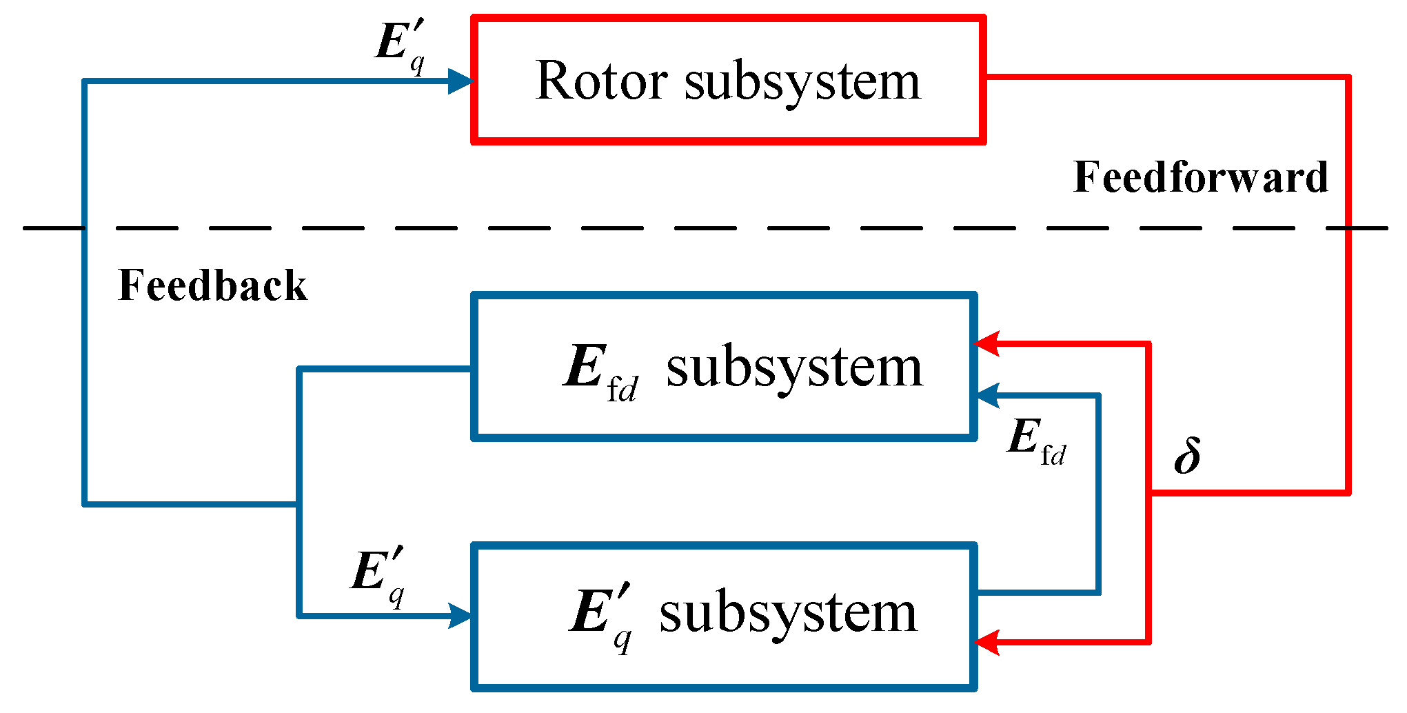
In general it is not a trivial task to study the properties of dynamic model (53). To gain insights into it, a decomposition-aggregation strategy has been suggested in [6]. Consider the rotor dynamics subsystem:

$$\left\{\begin{array}{cc}\hfill \dot{\mathsf{\delta }}& ={\omega }_0(\mathsf{\omega }-1)\hfill \\ \hfill 2\mathrm{H} \dot{\mathsf{\omega }}& ={\mathrm{P}}_{\mathrm{m}}-{\mathrm{K}}_q{\mathrm{E}}_q^{\prime }\circ {\mathrm{E}}_q^{\prime }-\mathrm{D}\mathsf{\omega }\hfill \end{array}\right.$$

(56)

Let us temporarily fix q-axis transient voltage E′q, then the rotor subsystem can be regarded as a Kuramoto model with E′q as an input. Similarly, the rotor angle $\mathsf{\delta }$ can be viewed as the input to the following subsystem:

$$\left\{\begin{array}{cc}\hfill {\mathrm{T}}_{d0}^{\prime }{\dot{\mathrm{E}}}_q^{\prime }& ={\mathrm{E}}_{\mathrm{f}d}-{\mathrm{E}}_q^{\prime }-({\mathrm{X}}_d-{\mathrm{X}}_d^{\prime }){\mathrm{K}}_d{\mathrm{E}}_q^{\prime }\hfill \\ \hfill {\mathrm{T}}_{\mathrm{A}}{\dot{\mathrm{E}}}_{\mathrm{f}d}& ={\mathrm{K}}_{\mathrm{A}}{\mathrm{V}}_{\mathrm{ref}}-{\mathrm{E}}_{\mathrm{f}d}-{\mathrm{K}}_{\mathrm{A}}\left|{\mathrm{V}}_{\mathrm{G}}\right|\hfill \end{array}\right.$$

(57)

It is interesting to observe that, the above voltage subsystem can be further decomposed into E′q subsystem and Efd subsystem. The readers are referred to [6,33,34,35] for details.

The above observations dictates that the dynamic model (53) exhibits a feedforward-feedback control structure, as depicted in Figure 11. The natures of the feedforward and feedback subsystems are distinctly different. This decomposition-aggregation strategy helps one to understand the dynamic behavior of power systems.

Naturally, one asks, what stability properties does the closed-loop system possess? Reference [6] provides some partial answers to this question. It should be noted that the property described in this section still holds true even if synchronous machines are represented by more complex salient models, see [6] for details.

3.6. Switched System Property

The model of a virtual synchronous machine (VSM) converter is quite similar to that of a synchronous machine, see [36,37,38,39]. When the grid experiences a severe fault, a VSM converter could activate a transient current limiting logic. This is an inherent characteristic that many power electronic devices possess, while traditional synchronous machines do not. Figure 12 below shows the model of such systems.

The model of the system immediately suggests that the behavior of such power systems involve switching, as Figure 13 demonstrates.

3.7. Augmented Synchronization Property

It was recently found that power system models often possess the so-called augmented synchronization. In a nutshell, the theory states that, under mild conditions, if the voltage of a power system converges, then the complete system is stable. The readers are directed to [40] for details about this insightful discovery.

We end this section by summarizing the properties described in this section as follows. The multi-stage property of power systems is very common, especially if a power system is disturbed by a three-phase-to-ground fault. The DAE and two-time-scale properties are also fundamental, virtually any realistic large-scale power system models have such properties. While the DAE properties increases the complexity in stability analysis, the two-time-scale property helps relieve the burden. Weakly nonlinear property is useful when studying frequency dynamics, it can also be useful in studying commutation failures. The interconnection property is less known, and it is most useful in understanding the role of subsystems. Switched system property is least understood, and it is attracting more and more research interests in recent years. Finally, augmented synchronization property reveals the fundamental synchronization problem in large-scale power systems and its implications can be far reaching.

4. Properties of the Subsystems

This section reviews the properties of the subsystems that were obtained using the decomposition strategies described in Section 3.

4.1. Properties of the Rotor Subsystem

In what follows, we briefly review the relevant properties of the rotor subsystem.

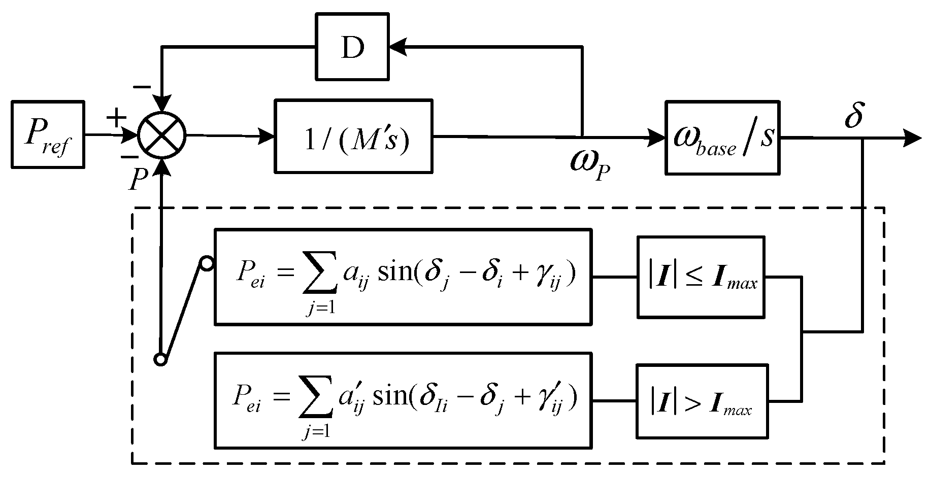
Let $Y=G+jB$ and ${\alpha }_{ij}=\angle Y_{ij}-\pi /2$. Introducing $K_{ij}=\left|E_{qi}^{\prime }{E}_{qj}^{\prime }{Y}_{ij}\right|$ and ${\Omega }_{ij}=P_{\mathrm{m}i}-D_i{\omega }_{\mathrm{ref}}-E_{qi}^{\prime }{E}_{qj}^{\prime }{G}_{ij}$, we obtain an alternative formulation of the subsystem:

$$2H_i{\ddot{\delta }}_i+D_i{\dot{\delta }}_i/{\omega }_{\mathrm{ref}}={\Omega }_i+{\displaystyle \sum _{j=1,j\ne i}^n{K}_{ij}\sin ({\delta }_j-{\delta }_i+{\alpha }_{ij})}$$

(58)

There exists extensive literature on the stability margin estimation of the above system; see, for instance [3]. The analytical expression of the stability region boundaries of the above system is addressed in [41].

Recently, it was found that there is striking similarity between the above model and the much studied Kuramoto model. A recent result, central in modern Kuramoto regime, is the following explicit formula for the estimation of stability region [42]:

$$L\sin {\Theta }_{\mathrm{c}}>\Theta (\Omega )$$

(59)

where L and $\Theta (\Omega )$ are explicitly defined in terms of system parameters. See [43] and references therein for some further results with similar flavor, and reference [44] for the development of an approach based on sum-of-square.

4.2. Properties of the Voltage Control Subsystem

Let us now re-write the voltage control subsystem (57) as follows:

$$\left[\begin{array}{c}{\mathrm{T}}_{d0}^{\prime }{\dot{\mathrm{E}}}_q^{\prime }\\ {\mathrm{T}}_{\mathrm{A}}{\dot{\mathrm{E}}}_{\mathrm{f}d}\end{array}\right]=\left[\begin{array}{cc}{\mathrm{K}}_{\mathrm{V}}& {\mathrm{I}}_n\\ 0& -{\mathrm{I}}_n\end{array}\right]\left[\begin{array}{c}{\mathrm{E}}_q^{\prime }\\ {\mathrm{E}}_{\mathrm{f}d}\end{array}\right]+\left[\begin{array}{c}0\\ {\mathrm{K}}_{\mathrm{A}}({\mathrm{V}}_{\mathrm{ref}}-\mathrm{h}({\mathrm{E}}_q^{\prime }))\end{array}\right]$$

(60)

where hi (∙) denotes a nonlinear function with $\partial \mathrm{h}/\partial {\mathrm{E}}_q^{\prime }\ge 0$; see [6] for more properties of the function.

One of the most interesting properties of (60) is that the Jacobian matrix J of the above subsystem exhibits a stable sign pattern. Taking the Jacobian matrix of the voltage subsystem of the 3-machine test system as an example, we obtain the following:

$$\mathrm{sgn}(\mathrm{J})=\mathrm{sgn}\left(\begin{array}{cc}{\displaystyle \frac{\partial {\dot{\mathrm{E}}}_q^{\prime }}{\partial {\mathrm{E}}_q^{\prime }}}& {\displaystyle \frac{\partial {\dot{\mathrm{E}}}_q^{\prime }}{\partial {\mathrm{E}}_{\mathrm{f}d}}}\\ {\displaystyle \frac{\partial {\dot{\mathrm{E}}}_{\mathrm{f}d}}{\partial {\mathrm{E}}_q^{\prime }}}& {\displaystyle \frac{\partial {\dot{\mathrm{E}}}_{\mathrm{f}d}}{\partial {\mathrm{E}}_{\mathrm{f}d}}}\end{array}\right)=\left[\begin{array}{cccccc}-& +& +& +& 0& 0\\ +& -& +& 0& +& 0\\ +& +& -& 0& 0& +\\ -& -& -& -& 0& 0\\ -& -& -& 0& -& 0\\ -& -& -& 0& 0& -\end{array}\right]$$

(61)

where sgn(∙) denotes the sign result; the symbol ‘+’ (‘−’, ‘0’) indicates that the entry is non-negative (non-positive, zero).

The sign pattern shown above illustrates that each entry of the Jacobian matrix is sign stable, indicating robust and well-behaved interactions among state variables. For instance, a rise in one transient voltage will elevate all the other transient voltages but reduce all excitation voltages. Additionally, all negative diagonal entries are conducive to the stability of the voltage dynamics.

The sign pattern of the Jacobian matrix J can be further probed as follows. One can easily construct the following augmented system to analyze voltage stability:

$$\left[\begin{array}{c}{\mathrm{T}}_{d0}^{\prime }{{\dot{\mathrm{E}}}_q^{\prime }}^{+}\\ {\mathrm{T}}_{\mathrm{A}}{\dot{\mathrm{E}}}_{\mathrm{f}d}^{+}\\ {\mathrm{T}}_{d0}^{\prime }{{\dot{\mathrm{E}}}_q^{\prime }}^{-}\\ {\mathrm{T}}_{\mathrm{A}}{\dot{\mathrm{E}}}_{\mathrm{f}d}^{-}\end{array}\right]=\left[\begin{array}{cccc}{\mathrm{K}}_{\mathrm{V}}& {\mathrm{I}}_n& 0& 0\\ 0& -{\mathrm{I}}_n& 0& 0\\ 0& 0& {\mathrm{K}}_{\mathrm{V}}& {\mathrm{I}}_n\\ 0& 0& 0& -{\mathrm{I}}_n\end{array}\right]\left[\begin{array}{c}{{\mathrm{E}}_q^{\prime }}^{+}\\ {\mathrm{E}}_{\mathrm{f}d}^{+}\\ {{\mathrm{E}}_q^{\prime }}^{-}\\ {\mathrm{E}}_{\mathrm{f}d}^{-}\end{array}\right]+\left[\begin{array}{c}0\\ {\mathrm{K}}_{\mathrm{A}}({\mathrm{V}}_{\mathrm{ref}}-\mathrm{h}({{\mathrm{E}}_q^{\prime }}^{-}))\\ 0\\ {\mathrm{K}}_{\mathrm{A}}({\mathrm{V}}_{\mathrm{ref}}-\mathrm{h}({{\mathrm{E}}_q^{\prime }}^{+}))\end{array}\right]$$

(62)

It is shown in [6] that an explicit estimate of stability region can be derived from the above augmented system.

Furthermore, the voltage subsystem can be decomposed into two monotone input–output control systems, as depicted below:

$$\left\{\begin{array}{cc}\hfill {\mathrm{T}}_{d0}^{\prime }{\dot{\mathrm{E}}}_q^{\prime }& ={\mathrm{K}}_{\mathrm{V}}{\mathrm{E}}_q^{\prime }+{\mathrm{u}}_1\hfill \\ \hfill {\mathrm{u}}_1& ={\mathrm{y}}_2={\mathrm{E}}_{\mathrm{f}d}\hfill \\ \hfill {\mathrm{y}}_1& ={\mathrm{E}}_q^{\prime }\hfill \end{array}\right.$$

(63)

$$\left\{\begin{array}{cc}\hfill {\mathrm{T}}_{\mathrm{A}}{\dot{\mathrm{E}}}_{\mathrm{f}d}& =-{\mathrm{E}}_{\mathrm{f}d}+{\mathrm{K}}_{\mathrm{A}}[{\mathrm{V}}_{\mathrm{ref}}+ \mathrm{h} \prime ({\mathrm{u}}_2)]\hfill \\ \hfill \mathrm{h} \prime ({\mathrm{u}}_2)& =-\mathrm{h}(-{\mathrm{u}}_2)\hfill \\ \hfill {\mathrm{u}}_2& =-{\mathrm{y}}_1=-{\mathrm{E}}_q^{\prime }\hfill \\ \hfill {\mathrm{y}}_2& ={\mathrm{E}}_{\mathrm{f}d}\hfill \end{array}\right.$$

(64)

It appears that the E′q subsystem and Efd subsystem exhibit the so-called static input-state characteristic, indicating monotonic changes in steady state with respect to the inputs [34,45]. A nice consequence of this fact is that one can conclude the asymptotic stability of the equilibrium of the above system in a constructive manner. The readers are directed to [46,47] for more discussions on the study of the voltage control subsystem.

4.3. Quasi-Linear Property of the Rectifier Model During Commutation Failures

When studying commutation failure, the mathematical model of the rectifier control system during commutation failure can be summarized as follows:

$$\begin{array}{l}{T}_{Idcmes}{\dot{I}}_{dcmes}=I_{dc}-I_{dcmes},\\ T_{VDCOL}{\dot{V}}_{dcImes}=V_{dcI}-V_{dcImes}\\ T_{IdR}{\dot{x}}_{Id}=I_{ord}-I_{dcmes}, \\ \alpha =\pi -[x_{Id}+k_{IdR}(I_{ord}-I_{dcmes})]\\ V_{dco}=V_{dcImes}+R_d/2\cdot I_{dcmes}, \\ I_{ord}=f_{VDCOL}(V_{dco})\end{array}$$

(65)

where TIdcmes is the time constant of the DC current measurement module. TVDCOL is the time constant of the DC voltage measurement module at the inverter side. As VdcI will drop to zero during a commutation failure, the time constant corresponding to the fall stage in VDCOL is chosen as TVDCOL. The meanings of the other variables can be found in [8].

Synchronous machines are represented by the same model as described in the previous sections. The network equation of the AC-DC system is as follows:

$$\left[\begin{array}{cc}{Y}_{GG}& Y_{GDC}\\ Y_{DCG}& Y_{DC}\end{array}\right]\left[\begin{array}{c}{V}_G\\ V_{comR}\end{array}\right]=\left[\begin{array}{c}-j{{X^{\prime }}_d}^{-1}(E_q^{\prime }\circ e^{j\delta }-V_G)\\ I_{comR}\end{array}\right]$$

(66)

where YGG, YDC, YGDC, and YDCG represent the submatrices of the network admittance matrix with respect to generator nodes and commutation bus. IcomR is the nodal injecting current of the rectifier commutation bus.

Again, as described in the previous sections, one can divide the complete AC-DC system into the fast subsystem, consisting of mainly HVDC state variables $\{I_{dc},I_{dcmes},V_{dc\mathrm{Im}es},x_{Id},E_{fd}\}$, and the slow subsystem, consisting of the variables of machines, such as $\{\delta ,\omega ,E_q^{\prime }\}$.

For the slow time-scale part of DC current ${\underset{\_}{I}}_{dc}$, due to VDCOL limits, it is regulated to the minimum current order in the fast equilibrium manifold, as follows:

$${\underset{\_}{I}}_{dc}={\underset{\_}{I}}_{ord}=Y_1$$

(67)

As a result, the DC current can be approximated by $I_{dc}\approx {\underset{\_}{I}}_{dc}+{\widehat{I}}_{dc}=Y_1+{\widehat{I}}_{dc}$, indicating that the fast time-scale part of DC current ${\widehat{I}}_{dc}$ is the only variable determining the actual dynamic DC current response.

The above arguments show that one only needs to examine the reduced-order fast subsystem to investigate the dynamics of DC current.

Now, let us proceed to simplify the set of network equations. Eliminating the generator nodes with Kron reduction, it follows that

$$I_{comR}=-j{X_d^{\prime }}^{-1}{Y}_{DCG}{Y_{GG}^{\prime }}^{-1}{E}_q^{\prime }{e}^{j\delta }+Y_{DC}^{\prime }{V}_{comR}$$

(68)

where ${Y^{\prime }}_{GG}=Y_{GG}-j{X_d^{\prime }}^{-1}$,$Y_{DC}^{\prime }=Y_{DC}-Y_{DCG}{Y_{GG}^{\prime }}^{-1}{Y}_{GDC}$. Let $Z_{eq}={Y_{DC}^{\prime }}^{-1}$ be the equivalent impedance of the AC system at rectifier node. Let $E_{eq}=j{X_d^{\prime }}^{-1}{Z}_{eq}{Y}_{DCG}{Y_{GG}^{\prime }}^{-1}{E}_q^{\prime }{e}^{j\delta }$ be the equivalent AC voltage source. Under the fast time-scale, $E_{eq}$ is viewed as a constant variable because the slow state variables $E_q^{\prime }$ and $\delta$ are fixed to their respective initial states. Substituting the expressions of Zeq and Eeq into (68), one obtains the following:

$$E_{eq}+Z_{eq}{I}_{comR}=V_{comR}$$

(69)

During a commutation failure, the DC power drops rapidly. As a result, the rectifier behaves more like a reactive load with the power factor angle reaching about 90 degrees. Notice that $I_{comR}=k_R{I}_{dc}$, and the above discussion suggests that

$$\left|V_{comR}\right|\approx \underset{E_{DC}}{\underbrace{\left|E_{eq}\right|\cos ({\theta }_E-{\theta }_V)}}-\underset{k_{DC}}{\underbrace{\left|Z_{eq}\right|k_R\sin {\theta }_Z}}{I}_{dc}$$

(70)

where ${\theta }_E$, ${\theta }_V$, ${\theta }_Z$ are the phase of equivalent voltage sources of the AC grid, the phase of rectifier bus voltage, and the phase of the equivalent impedance, respectively.

Notice that ${\underset{\_}{I}}_{dc}={\underset{\_}{I}}_{dcmes}=Y_1$; it follows ${\widehat{I}}_{dc}=I_{dc}-Y_1$,${\widehat{I}}_{dcmes}=I_{dcmes}-Y_1$. Finally, we obtain the decoupled fast subsystem as follows:

$$\begin{array}{l}{L}_d^{\prime }{\displaystyle \frac{d{I}_{dc}}{d\tau }}=k_R(E_{DC}-k_{DC}{I}_{dc})\cos \alpha -(X_{cR}+R_d)I_{dc},\\ T_{Idcmes}^{\prime }{\displaystyle \frac{d{I}_{dcmes}}{d\tau }}=I_{dc}-I_{dcmes}, \\ T_{VDCOL}^{\prime }{\displaystyle \frac{d{V}_{dcImes}}{d\tau }}=-V_{dcImes},\\ T_{IdR}^{\prime }{\displaystyle \frac{d{\widehat{x}}_{Id}}{d\tau }}=I_{ord}-I_{dc},\alpha =\pi -[{\widehat{x}}_{Id}+{\underset{\_}{x}}_{Id0}+k_{IdR}(I_{ord}-I_{dcmes})].\end{array}$$

(71)

where $L_d^{\prime }=L_d/\epsilon$ is scaled, so are the other integral constants.

In fast subsystems (71), the range of α is [15°,100°]. Within this range, cosine function can be approximated by a linear function as $\cos \alpha \approx k_1\alpha +b$, with $k_1=-0.77$, $b=$ 1.26. A similar linearization method has been applied in [48], and the linear fitting result is shown in Figure 14.

Notice that $k_{DC}$ is generally a small parameter, which is typically smaller than 0.3. Let $\sigma =k_{DC}$, substituting $k_1\alpha +b$ into (71); one obtains a weakly nonlinear system for approximating the DC current. A simple approach to obtaining an analytical solution for this weakly nonlinear system is described in [8], based on the standard theory of regular perturbation.

5. Conclusions

Depending on the system conditions, a power system can exhibit highly complex and diverse behaviors during transient periods. In this work, we demonstrate such behaviors using MATLAB simulation tools developed by the authors. We summarize and investigate the analytical properties of power system models, aiming to establish a connection between these complex behaviors and the underlying mathematical representations. Notably, several analytical tools—inspired by a divide-and-conquer strategy—prove both available and effective for understanding transient dynamics in power systems. We believe that further research in this direction will yield valuable and insightful results.