Abstract
The environmental impact of innovative indirect regenerative evaporative cooling (IREC) technology is analyzed using the life cycle assessment. This study compared typical equipment using this technology from Innovative Ideas LLC with available-on-the-market traditional vapor compression ducted air conditioning systems as the closest analogous representatives of the vapor compression technology. For comparison, units with the same cooling capacity (5 kW) were selected. The endpoint indicators demonstrated that the air conditioning systems using IREC technology had lower environmental load compared to the vapor compression system by 29–70%, depending on the scenario and damage category. This advantage resulted from the significantly higher coefficient of performance of the IREC system. The amounts of cooling energy generated and electricity consumption were determined based on temperature and relative humidity data recorded at hourly intervals in the summer seasons of 2023 and 2024. The operation turned out to be a life cycle stage with dominating environmental load. The uncertainty analysis carried out with Monte Carlo simulations indicated significant deviation, particularly for the ecosystem category. The sensitivity analysis showed that the assumed electricity mix did not significantly affect the general conclusions.
1. Introduction
The continuous rise in energy consumption due to the increasing demand for air conditioning (AC) in the residential, commercial, and industrial sectors poses significant environmental challenges, particularly in terms of greenhouse gas emissions and the depletion of energy resources. Consequently, the development and adoption of energy-efficient and environmentally friendly cooling technologies have become essential. Two primary technologies currently dominate the air conditioning market, traditional vapor compression air conditioning systems and evaporative cooling systems, including the innovative indirect regenerative evaporative cooling (IREC), also known as the Dew Point Indirect Evaporative Cooler (DPIEC), often based on the Maisotsenko cycle (M-cycle) [1,2,3].
Air conditioning systems that use vapor compression refrigerating machines (VCRMs) have been widely utilized for decades due to their capability to maintain stable indoor temperatures, irrespective of ambient humidity [4,5,6,7,8,9,10]. Such systems utilize refrigerants in vapor compression cycles involving compression, condensation, expansion, and evaporation processes. Commonly used refrigerants include synthetic hydrofluorocarbons (HFCs), with R-134a, R-410A, and R-32 being notable examples [11,12,13]. However, despite their widespread adoption and reliability, vapor compression systems exhibit significant environmental impacts, attributed to high energy consumption and refrigerant leakage [14,15]. To address these issues, alternative refrigerants and energy-saving innovations such as variable-speed compressors, electronic expansion valves, and advanced control systems have been introduced. Moreover, vapor compression systems possess reversibility, allowing operation as heat pumps for space heating during colder periods, enhancing their overall utility and cost-effectiveness [4].
On the other hand, evaporative cooling technologies, particularly indirect evaporative coolers based on the Dew Point principle (DPIEC), present promising alternatives due to their significantly lower electrical energy consumption and elimination of harmful refrigerants [16,17,18,19]. These systems use a special heat exchanger design that makes cooling possible below the wet-bulb temperature through water evaporation and a specialized flow regime. This is a big deal as it means that the temperature difference between the dew point and wet bulb can reach over 10 °C, depending on weather conditions. The Maisotsenko cycle (M-cycle), a special implementation of IREC, has been proven highly effective in achieving air temperatures near the ambient air dew point temperature without increasing air humidity in the product air stream [20,21,22,23]. IREC systems are especially advantageous in hot and dry climates, offering substantial reductions in energy consumption compared to vapor compression systems [24,25,26]. Nevertheless, their effectiveness declines significantly in highly humid conditions, limiting their broader application without supplementary dehumidification [27,28,29]. Additionally, the IREC system requires access to a local water source; therefore, its operational convenience and maintenance requirements can be significantly influenced by water quality. For example, if the water source is remote, it becomes necessary to install pipelines to supply water to the system. Furthermore, poor water quality may result in the accumulation of salts and other contaminants on the heat exchange surfaces, necessitating more frequent cleaning of the heat exchanger core. The abovementioned factors may confine the domain of use for IREC AC systems.
Recent advancements propose hybrid systems, integrating desiccant-based dehumidification units with IREC technology to overcome the limitations associated with high ambient humidity. Such hybrid systems utilize adsorbent materials, including traditional silica gel and innovative metal–organic frameworks (MOFs) like MIL-101-Cr, to effectively manage indoor humidity while maintaining low energy consumption [30,31]. In particular, Harrouz et al. [32] demonstrated the feasibility of such hybrid systems in hot and humid climates, achieving up to 48% and 17% reductions in electrical and thermal energy consumption, respectively, compared to traditional silica gel desiccants.
The literature analysis shows that IREC (or DPIEC, M-cycle) became more popular in the mid-2010s. The Web of Science database has indexed 770 scientific documents concerning the topic, so far. Despite unquestionable advantages identified associated with high energy efficiency, few articles have addressed the quantification of environmental benefits resulting from this potential. Queries including life cycle assessment or carbon footprint of the concerned technology indicated only three articles, summarized below.
Harrouz et al. [32] proposed integrating a water reclamation unit with desiccant–dew point evaporative cooling systems to reduce water consumption in poultry houses in hot, humid climates. Two desiccants, silica gel and MIL-101-Cr, were evaluated through numerical modeling, artificial neural networks, and system optimization for a case study in Qatar. Although the study title literally includes the name life cycle assessment method, the study actually conducted a life cycle cost analysis, demonstrating MIL-101-Cr to be more cost-effective despite its higher initial cost.
Tariq et al. [33] investigated a novel mixed-flow air saturator configuration within the Maisotsenko Humid Air Bottoming Cycle to enhance waste heat recovery in gas turbine power plants. Utilizing a hybrid cross-flow and regenerative counter-flow heat and mass exchanger, the system achieves up to 57 MW of output and 42% thermal efficiency, outperforming traditional counter-flow setups. Notably, the proposed configuration results in an approximately 55% lower carbon footprint compared to the conventional counter-flow air saturator.
Alam et al. [34] analyzed dew point evaporative cooling systems, highlighting advancements in heat and mass exchangers, wetting materials, and optimization techniques that significantly improve system performance and energy efficiency. The authors emphasized the potential of hybrid systems integrated with liquid desiccant or vapor compression systems to reduce building energy consumption up to 84%. Although the study emphasizes the potential of the analyzed systems to achieve near-zero-carbon emissions, it does not include a quantitative analysis of the carbon footprint or greenhouse gas emissions.
A comparison of the VCRM with different heat-driven refrigeration systems (absorption system and ejector system) in terms of carbon footprint was presented in [35]. The heat-driven cooling systems indicated lower environmental impact by 59–68% compared to the vapor compression system. The difference significantly depended on the country and its corresponding national electricity emission factor.
Given the results of the state-of-the-art analysis in the field of indirect regenerative evaporative cooling, a literature gap regarding the determination of the environmental impact of this technology has been identified. Considering the energy reduction potential provided by IREC, improved performance during the use phase compared to VCRM systems might be expected. However, quantifying the magnitude of this benefit in relation to other life cycle processes requires an assessment of the amount of materials involved in the manufacturing phase and end of life of the AC units concerned. The novelty of this study lies in its comprehensive LCA-based comparison of IREC and VCRM systems, which has not been previously addressed in the literature. Accordingly, the main objective is to compare the environmental impacts of the IREC and VCRM systems. This goal will be achieved by applying life cycle assessment, which is a recognized decision-support tool in various fields of energy-related sectors, including air conditioning [36,37].
2. Materials and Methods
2.1. Method of Assessing Environmental Impact
As mentioned in the Introduction, the main objective of this study was to determine the environmental impact of the IREC AC system and compare it with the corresponding impact of the duct VCRM AC system. In order to enhance the reliability of the comparison, various VCRM scenarios are considered, including different approaches for electricity consumption calculations as well as alternative electricity mix. LCA method was applied to determine the environmental indicators.
The environmental impact of the analyzed products to be compared was determined using life cycle assessment method in accordance with the standards (ISO 14040 and ISO 14044 [38,39]). The subsequent phases of LCA framework (goal and scope definition, inventory analysis (LCI), impact assessment (LCIA) and interpretation) are included in Section 2 and Section 3.
The boundaries of the systems were defined according to a cradle-to-grave approach. The product systems included natural resource extraction processes, transportation and processing of raw materials, electricity generation, and end of life. The functional unit was defined as a single device providing cooling energy to decrease the temperature of fresh air flow to 19 °C in summer seasons over a period of 10 years. Data for IREC prototype AC unit were provided by Innovative Ideas LLC. Taking into consideration that IREC presumes the use of air ducts to deliver cooled air to the consumer, the relevant ducted VCRM air conditioning technology was chosen for comparison. Both the compared units perform both cooling and ventilation functions. Data for the VCRM system were obtained from various publicly available sources containing details on a variety of equipment offered by the AC market. The source of the secondary process data was the ecoinvent 3.8 database [40]. The datasets for LCI stage for both analyzed systems are presented in Table 1 and Table 2.

Table 1.
Amounts of materials used for VCRM system manufacturing.
Table 2.
Amounts of materials used for IREC system manufacturing.
The impact assessment phase was carried out using ReCiPe Midpoint (H) as well as ReCiPe Endpoint (H) methods [41].
The development of product system models adopted the following assumptions:
- A constant volumetric fresh air flow amounting to 800 m3/h was assumed.
- The lifespans of the compared products and, consequently, their operation periods are the same (summer seasons over 10 years).
- After the operation period, both units will be recycled.
- The outside air parameters for the operation time were based on the measurements for May–September period in 2023 and 2024.
- Following the provisions of ISO 14044 standard, saying that exclusion of given processes is permitted if it does not significantly change the general conclusion of the analysis, the installation elements of the cooling systems (pipe connections, cables, etc.) were excluded from the product system boundaries as identical for both compared scenarios.
- The analyses adopted mass (physical) allocation approach.
- The LCIA procedures were carried out using cutoff parameter of 0.0001, meaning that the processes with the contribution to total impact smaller than 0.01% were neglected.
- The uncertainty analysis was carried out by means of Monte Carlo simulations with 5000 iterations. Input parameters were assigned lognormal distributions based on the uncertainty factors available in the ecoinvent 3.8 database. Output results were presented as the confidence intervals for 5th and 95th percentiles obtained for individual endpoint categories.
- Since AC units are assumed to be operated in the city of Sumy (using historical statistical data as input conditions), the Ukrainian electricity mix was adopted.
- The initial amount of the refrigerant (R-32) necessary for operating VCRM was 1.075 kg, including 50 g per meter of 3.5 m connecting installation.
- Length of air ducts for both systems is equal and comprises 15 m.
- 5 kW AC unit passport specifications and a targeted supply flow rate of 800 m3/h of cooled air to the consumer were assumed for both systems. Notably, the energy efficiency of evaporative cooling units grows more intensively with the increase in the installed cooling capacity compared to VCRM.
- The leakage of the refrigerant was assumed to be 1.12% per year [42].
- A building for the installed AC system is a thermally well insulated changing room of a sports hall, with no extra heat fluxes except internal sources.
2.2. Data Collection
Experimental data for IREC at various ambient air parameters and materials used in its design were provided by the company Innovative Ideas LLC (Sumy, Ukraine) [43]. The company’s product prototype (Figure 1) examined in this study is similar to the closest commercially available products from companies such as Seeley International. The principle of operation of this indirect regenerative evaporative cooling apparatus is as follows:
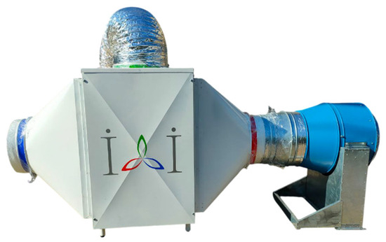
Figure 1.
Photo of the considered IREC system.
- Air from the environment is supplied by a fan into the apparatus and is then divided into two components.
- The working flow passes through a system of dry channels (where it transfers heat to the adjacent wet channels and is cooled at constant moisture content) and then through wet channels (where the air is heated and saturated with water vapor at a constant relative humidity, RH).
- Meanwhile, the second component of the incoming air flow is the product flow (cooled air delivered to the consumer). Passing through its set of dry channels, the product flow gives off its heat to the wet channels and, thus, cools at a constant moisture content.
Because of its design features, the device can cool air to the wet-bulb temperature and even slightly below it under certain inlet air conditions (approaching the dew point as the theoretical limit). The prototype shown in Figure 1 consists of two heat and mass exchange (HMX) cores. Each HMX core is designed to produce about 460 m3/h of cooled air plus 340 m3/h of 100% humid air, with a total of 800 m3/h of outside air. In practical applications, 3 to 6 such cores can be integrated into a single unit, with multiple apparatuses arranged in modular fashion in quantities required to cool the desired volume of air.
The data on energy efficiency and materials for a typical VCRM system (Figure 2) were collected from the official websites of the respective duct AC manufacturers (e.g., Daikin, Fujitsu, Hitachi, Samsung, Haier, LG, Mitsubishi Electric, etc.), reports, standards and guidelines on the regulation and energy efficiency improvements of air conditioning systems with low global warming potential (GWP). In addition, data from relevant scientific publications concerning the analysis, prediction and efficiency improvement of classical compressor air conditioning systems were analyzed [44,45,46,47,48].
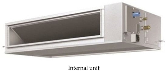
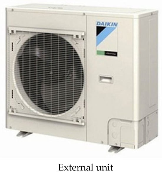
Figure 2.
External and internal units, refrigerant and electric line installation of typical VCRM ducted AC system.
Components and operating principles of VCRM system for ducted AC can be shortly described as follows: a vapor compression refrigeration system (VCRS) is a cooling technology widely employed in duct air conditioning systems, owing to its capacity to provide precise and stable temperature control, regardless of ambient humidity conditions. The primary components of a typical vapor compression refrigeration cycle include a compressor, condenser, expansion device, and evaporator, integrated into a closed-loop system charged with refrigerant.
2.3. Historical Climate Data for the Considered Region
To evaluate the performance of the compared AC systems, historical meteorological data for Sumy, Ukraine, were obtained from the Meteostat website [49]. These data cover the period from May to September for the years 2023 and 2024, with measurements recorded at hourly intervals (Figure 3). This dataset includes key environmental parameters, such as temperature, dew point, relative humidity, precipitation, wind direction, and speed, atmospheric pressure, and cloud cover. These data were used as input conditions for the experimental evaluation of the IREC system efficiency, ensuring that the testing conditions represent real-world operating conditions.
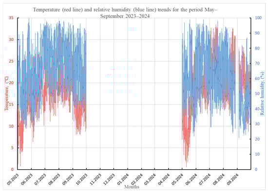
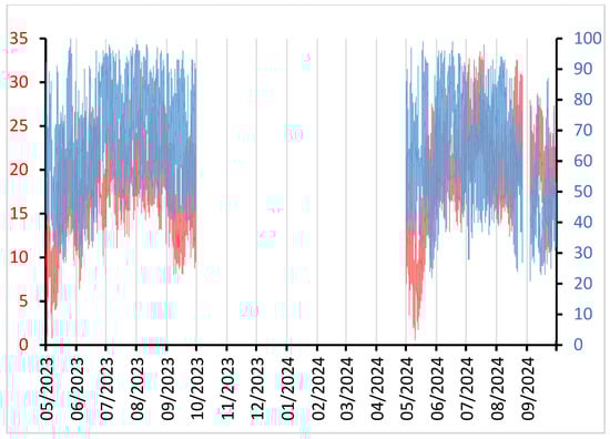
Figure 3.
Temperature and relative humidity trends (May–September 2023, 2024) recorded at hourly intervals.
The report by Innovative Ideas LLC supplements these historical environmental data to simulate the performance of the IREC prototype. Specifically, the report presents a scatter diagram illustrating the distribution of ambient temperature and relative humidity in Sumy during the spring–autumn periods of 2019 and 2020, with measurements taken at three-hour intervals (Figure 4). In Figure 4, the bold dots highlighted in black denote the most frequently occurring operating conditions for the region under consideration, as well as for occasional hot points where the device’s cooling effect is expected to be most pronounced. This visualization aids in understanding the climatic context within which the IREC system operates, thereby supporting a comprehensive evaluation of its performance.
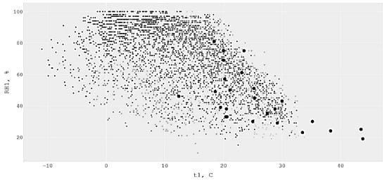
Figure 4.
Scatter diagram of ambient temperature and relative humidity distribution in Sumy city, spring–autumn 2019–2020, with a 3 h interval [43].
This methodology aligns with scientific best practices by ensuring that experimental results are grounded in real-world data, enhancing the validity and reliability of the performance assessments conducted for the IREC prototype.
Figure 5 shows an array of historical data points for the period May–September for 2023–2024 and highlights the most frequently occurring environmental parameters for the selected period (similar to the data presented in Figure 4). Gray dots represent all recorded data points. Black dots indicate the most frequently occurring temperature and humidity values for this region during the selected period.
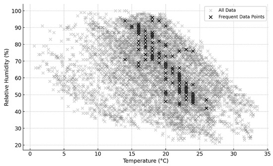
Figure 5.
Scatter diagram of temperature and relative humidity in Sumy for the period May–September for 2023 and 2024.
To confirm the regularity of the data presented above, the average monthly temperatures for the season in the range of 2021–2024 were calculated (Table 3) based on data from the original Meteostat website [49]. From the data in the table, it can be concluded that the historical data on environmental parameters reflect climatic patterns for the region under consideration, since deviations in the average monthly temperature are not significant, and the general trend towards its increase remains.
Table 3.
Average monthly temperatures in °C for the season in the range 2021–2024.
Evaluation of the IREC AC system characteristics relied on the results of experimental investigations conducted by II LLC for standard HMX core under steady conditions at the test rig inlet (temperature t, relative humidity RH, and volumetric flow = 800 m3/h). The results are presented in Table 4. During each test, the steady-state output parameters of the product flow (supplied cooled air) were measured. The electrical power N of fan and the water mass flow rate Gw supplied to the system were also recorded. The operating parameters were chosen partly based on statistical weather data for the target region (Sumy, Ukraine). The experimental data were used to analyze the cooling process efficiency relative to the wet-bulb and dew point temperatures for each mode.
Table 4.
Test results of heat and mass transfer core of the apparatus under various climate conditions from II LLC report [43].
A response surface was built on the basis of experimental points (black points shown on the surface in Figure 6). Using this surface, it is possible to estimate the output temperature (marked as t2) for other nearby or intermediate input parameters (marked as t1) and (marked as RH1), which are not presented in Table 4. To separate the area of reliable data, obtained using this surface, an auxiliary saturation surface (2) was constructed, corresponding to the theoretical limit of the outlet air temperature (dew point). In this case, the confidence zone of the response surface (1) is the portion located above the saturation surface.
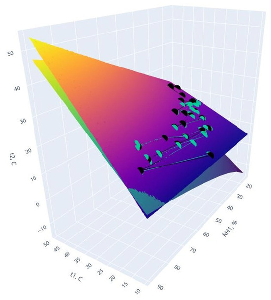
Figure 6.
Output temperature response surface t2 (1) depending on the input parameters t1 and RH1 [43].
Inverse Distance Weighted (IDW) interpolation was utilized for predicting IREC cooling capacity under outdoor conditions that deviate from those shown in Table 4. The methodology is a well-established spatial estimation approach, premised on the principle that the influence exerted by known data points on an unknown variable decreases as the spatial separation between them increases. Inverse Distance Weighted (IDW) interpolation technique is widely recognized in the field of spatial estimation for its simplicity, locality, and deterministic nature [50,51,52,53].
Two-Dimensional IDW Interpolation:
Given that the experimental design varies between two independent parameters, t1 and RH1, let: known input parameters for the i-th data point (from Table 4):
the corresponding measured outlet air temperature;
coordinates of a target point for interpolation;
predicted outlet temperature t2 at the target point.
The Euclidean distance from the interpolation point to the i-th known point is computed as:
Weights are assigned based on inverse distance raised to the power :
where is the power parameter, which emphasizes the influence of nearby points.
The interpolated outlet temperature is then:
Here, is the total number of known data points, or, alternatively, nearest neighbors may be used. The power controls the rate at which influence diminishes with distance. Typical values are (linear decay) or (quadratic decay).
2.4. Method for Assessing and Predicting the Cooling Capacity and Energy Efficiency of Vapor Compression Evaporative Cooling Systems
The assessment and prediction of the cooling capacity and energy efficiency of vapor compression refrigeration machines (VCRMs) and evaporative cooling systems require a systematic approach that incorporates thermodynamic modeling, experimental validation, and statistical analysis. This section outlines the methods employed to evaluate the performance of these systems, ensuring that results are scientifically robust and practically applicable.
Cooling Capacity Assessment
The cooling capacity of a VCRM is determined using the enthalpy difference method, which relies on the thermodynamic properties of the refrigerant. The equation is given as:
where: —mass flow rate of the refrigerant (kg/s); —enthalpy of the refrigerant at the evaporator inlet and outlet, respectively (J/kg). Data for enthalpy values can be obtained from refrigerant property tables or real-time measurements from pressure–enthalpy (P-h) diagrams.
Coefficient of Performance and Energy Efficiency Ratio Analysis
The coefficient of performance (COP) for VCRM units is defined as:
where: —VCRM AC unit power input (W).
Determining the power consumption of a 5 kW cooling capacity of VCRM AC unit requires understanding its energy efficiency ratio (EER), which is defined as the ratio of the cooling capacity to the electrical power input:
Given that 1 kW equals 3.412 BTU/h, a 5 kW unit has a cooling capacity of 5∙3.412 = 17.06 BTU/h. Rearranging the EER formula to solve for power consumption and taking into consideration statistical and experimental data provided in publications [14,44,45,46,48,54,55,56,57,58,59,60,61] concerning values of EER for VCRM, one can assume an EER of 11 (a common value for residential AC units), and the power consumption is:
Therefore, the unit would consume approximately 1.55 kW under nominal operating mode at 35 °C 50% relative humidity. This section includes sample calculations to justify the assumptions made. The obtained result reflects the average statistical data for ducted AC unit. For instance, power for AUX-C-18CAD unit (AUX, Ningbo, Zhejiang, China) consumption comprises 1.55 (0.47–2.3) kW.
The efficiency of AC units declines as outdoor temperatures rise, leading to increased power consumption, and, vice versa, as outdoor temperatures decrease, the heat load on the AC unit diminishes, resulting in reduced power consumption. For instance, research indicates that at an outdoor temperature of 28 °C, an inverter AC’s coefficient of performance (COP) can reach up to 5.2, compared to a COP of 2.34 for a non-inverter AC under the same conditions [62]. Both empirical studies and theoretical analyses [63,64,65] confirm that the power consumption of VCRM air conditioning units decreases by approximately 2% for each degree Celsius decrease in outdoor temperature below 35 °C. This relationship is crucial for optimizing the energy efficiency of air conditioning systems, especially in regions with significant temperature variations. Assuming a base power consumption of approximately 1.55 kW at standard conditions (as previously mentioned), and considering that power consumption decreases by approximately 2% for each degree Celsius decrease in outdoor temperature below 35 °C, the adjusted power consumption can be estimated using the following formula:
It must be emphasized that Equation (8) represents a linear approximation applicable solely for simplified computational analysis within the specified temperature range. This simplification does not disregard current scientific understanding but acknowledges the inherent complexity of real-world energy characteristics.
The performance metrics of VCRM systems, specifically cooling capacity (), power consumption (), and coefficient of performance (COP), demonstrate strong dependence on the following:
- Environmental parameters (ambient temperature, relative humidity);
- Operational configurations of equipment.
For instance, positioning the outdoor condensing unit on sun-exposed building surfaces (e.g., rooftops or south-facing walls) induces significant condensation temperature elevation. This results from combined solar irradiance and thermal emission from heated structural components, even at moderate ambient temperatures.
Analytical modeling of these multifactorial relationships remains challenging. Furthermore, existing research on temperature-dependent VCRM performance primarily focuses on the 24–38 °C range. Below this interval, nonlinear behavior in energy characteristics becomes increasingly probable, though insufficiently documented in the current literature. For instance, under ambient conditions approaching the target indoor temperature threshold, the coefficient of performance (COP) is expected to significantly exceed values derived from Equation (8). This deviation arises because reduced temperature differentials between evaporation and condensation phases substantially lower the compressor pressure ratio, thereby decreasing electrical energy consumption. Under such conditions, the system’s power demand theoretically reaches its minimum feasible value. As demonstrated by the aforementioned sample calculations of the AUX-C-18CAD unit, this corresponds to approximately 470 W. This discrepancy highlights the limitations of linear approximations for low-temperature regimes.
When selecting the target room temperature, data from the literature were considered [66,67]. For example, as noted in [67], the authors stated the following: “People who live in temperate climate zones generally find an indoor temperature range of 20–23 °C with a relative air humidity of 40–60% as comfortable. However, humans are also able to adapt temperatures by behavioral adjustment, physiological acclimatization, and psychological habituation or expectation. ASHRAE Standard 55 therefore specifies a range between approximately 67 °F and 82 °F (19.4–27.8 °C) for thermal comfort purposes of occupants.” Thus, the target room-temperature level in the article was set at 19 °C as the lowest comfort temperature level that can be provided by the considered AC systems.
For both types of air conditioners, the target room temperature (19 °C) also played the role of a limiting value for the ambient conditions during the comparison and calculation. Thus, when the ambient temperature is lower than the target room temperature, the air conditioners are not switched on, and, conversely, if the ambient temperature exceeds the target room temperature, the air conditioners are switched on. Therefore, the part of the statistical data that was limited, as well as the time when the air conditioners were not operating, was not included in the calculations for assessing the efficiency of the air conditioning systems under consideration.
To reduce this discrepancy, an alternative algorithm is proposed for assessing VCRM AC system efficiency. This algorithm places the VCRM AC unit into slightly more favorable conditions compared to the IREC AC unit but helps eliminate the risk of underestimating the VCRM AC unit’s efficiency at low ambient temperatures:
- 1.
- For the range from target room temperature 19 °C to 24 °C (due to the lack of experimental data), it is proposed to accept COP value at the maximum feasible level for the VCRM unit considered:
For a temperature range from 24 °C to 35 °C, it is proposed to accept value at 5 as the best level for the inverter VCRM AC unit [62].
For the rest of the range from 35 °C, it is proposed to use Equations (5) and (8).
Note: Based on the results of multiple calculations for this method, it is possible to accept, with high reliability, an average performance coefficient of 5 () for the entire temperature range under consideration.
- 2.
- For the actual ambient temperature, the actual cooling capacity of the VCRM AC unit is calculated to supply the required 800 m3/h of cooled air to the consumer:where is the mass flow rate of the supplied air, is the specific heat capacity of the supplied air, is primary air dry-bulb temperature at VCRM AC unit input (this temperature is equal to ambient temperature as a rule), is dry-bulb temperature of the supplied cooled air at VCRM AC unit output. For the considered calculation method, .
- 3.
- The specific power consumption of the air conditioning system per 1 degree Celsius is calculated at a given mass flow rate and a given coefficient of performance or for the corresponding temperature ranges:
- 4.
- The total cooling energy of the VCRM AC unit is calculated for the considered time period of historical data, :
- 5.
- Energy expended on the operation of VCRM AC to achieve the target temperature for the i-th time interval of historical data, , is as follows:
- 6.
- The total energy consumption the VCRM AC unit is calculated for the considered time period of historical data, :
- 7.
- The reduced seasonal performance coefficient of the VCRM AC plant was calculated as follows:
Note: Since the algorithm proposed by the authors for calculating the seasonal performance coefficient for VCRM of AC installations differs from the method described in the BS EN 14825:2022 [68] standard, it is proposed to use the designation as for the reduced seasonal performance coefficient in the following text.
2.5. Method for Assessing and Predicting the Cooling Capacity and Energy Efficiency of IREC Cooling Systems
Assessment of cooling capacity of IREC cooling system was fulfilled with regard to the provided comprehensive experimental data (Table 4) from Innovative Ideas LLC and can be calculated using the following equation:
where is the mass flow rate of the supplied air, is the specific heat capacity of the supplied air, is primary air dry-bulb temperature at IREC AC unit input, is dry-bulb temperature of the product flow (supplied cooled air) at IREC AC unit output.
The power input of the IREC AC unit is the sum of the power consumed by the fan , water pump (if there is no central water supply), electronic controls and surfactant dispenser . The last two components contribute negligibly to the total power consumption of the installation. Therefore, one can write:
For the case considered in the current study, , as for the IREC AC unit with central water supply system. The problems of condensation and return (recirculation) of evaporated water in the IREC system were not considered, since the objective of this study was to compare the basic IREC installation to traditional VCRM systems. Since there are many engineering solutions to the problem of recirculation of a part of evaporated water, their consideration exceeds the scope of this study and is of interest for a separate future study.
The effectiveness of an evaporative cooling system is commonly assessed by comparing the actual cooling achieved to the theoretical cooling potential based on wet-bulb and dew point temperatures.
where: —wet-bulb temperature at the device inlet conditions (°C), —dew point temperature at the device inlet conditions (°C). A higher or indicates better performance.
The total cooling energy of the IREC AC unit is calculated for the considered time period of historical data, :
where —cooling capacity of the IREC AC unit for the i-th time interval, —duration of the i-th time interval.
Energy expended on the operation of IREC AC to achieve the target temperature for the i-th time interval of historical data, , is as follows:
The total energy consumption of the IREC AC unit is calculated for the considered time period of historical data, :
The reduced seasonal performance coefficient of the IREC AC plant was calculated as:
To clearly refer to the compared systems and their further modifications, the baseline scenarios were designated as IREC1 and VCRM1. For both scenarios, the total amount of cooling energy as well as total electricity consumption determined for the analyzed summer periods of 2023 and 2024 are presented in Table 5. A comparison of electricity consumed over the entire period assumed in the analyzed scenarios is shown in Figure 7.
Table 5.
Total amounts of cooling energy and electricity consumption for May–September of 2023 and 2024 for IREC1, VCRM1 and VCRM2 scenarios.
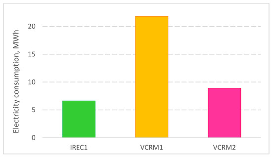
Figure 7.
Total electricity consumption for 10-year operation of the analyzed systems.
The energy calculations for VCRM1 considered real operational characteristics of the system with respect to changes in environmental conditions, as described in Equation (8). The cooling energy provided by IREC system is insignificantly smaller (0.44%) compared to the VCRM system that is due to the limited ability to generate cooling under the least favorable meteorological conditions (high humidity). Additionally, the VCRM2 scenario was analyzed assuming the AC system COP at an average level of 5 that corresponds to the highest attainable values for the considered type of system. In order to examine the effect of greener-energy powering equipment on study results, the scenarios IRECeur and VCRMeur assuming European electricity mix were also analyzed.
3. Results and Discussion
Table 6 presents midpoint indicators for the analyzed scenarios. For all impact categories considered, VCRM demonstrates a significantly higher (3–4-times in most cases) environmental impact compared to the IREC system. This observation is confirmed by Figure 8, which depicts relative damage indicators obtained for both scenarios broken down into the main life cycle stages, where 100% indicates the total VCRM1 impact for a given endpoint category. The electricity consumption (denoted in Figure 8 by ‘el’) for the VCRM system operation turned out to have the highest impact, regardless of the category. This single process is responsible for 88–95% of the total environmental impact attributable to ducted compressor AC. The analogous indicators of electricity used by the IREC system are around 3.3-times lower compared to the VCRM1 scenario. The distinct advantage of the IREC1 scenario over the traditional system results mainly from the difference in COP for both solutions that amounted to 3.48 compared to 1.06, respectively. However, also in the IREC1 case, energy consumed for operation is the most burdensome process in this scenario, with the impact contribution ranging 86–93% depending on the endpoint category. The advantage associated with electricity consumption has crucial significance due to the operation stage lasting over the entire lifespan of the products.
Table 6.
Midpoint characterization indicators for the life cycle of IREC1 and VCRM1 scenarios.
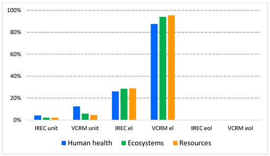
Figure 8.
Relative endpoint indicators for the selected life stages of IREC1 and VCRM1 scenarios: unit—production stage; el—electricity consumption for operation; eol—end of life.
The phase of the life cycle with the second highest environmental impact in the scenarios is the production (in Figure 8 referred to as ‘unit’) of the air conditioning unit, including raw material extraction, processing, and manufacturing processes. For the VCRM1 scenario, the contribution of this phase to the total impact amounted to 5–12% depending on the damage category. In the case of the IREC1 scenario, the contribution was at a comparable level, ranging 7–14%. For both scenarios, the greatest contribution was identified for the human health category, while for ecosystems and resources, the contribution was approximately two-times lower. It should be emphasized that production of the VCRM unit showed a 2.1–3.0-times higher environmental burden compared to the IREC unit. The reason for this difference is the amounts and types of the materials used for both units. The IREC system benefited from the relative simplicity of the unit’s construction. The third life cycle phase indicated in Figure 8 is the end of life, denoted by the acronym ‘eol’. However, the contribution of this phase to the total impact of the analyzed scenarios was below 0.2%; hence, there are no visible bars in Figure 8 in the ‘eol’ sections.
For both analyzed scenarios, the environmental burden was dominated by impacts within certain midpoint categories: global warming (attributable to 53% of damage to human health and 77% to ecosystems) and fossil resource scarcity (attributable to 98% of damage to resources). An example process network for the VCRM1 scenario, focusing on global warming, is depicted in Figure 9. The flow distributions confirm that the greatest impact results from electricity consumption, while the most impactful manufacturing processes (the production of electronic components and copper parts) each contributed less than 1%. Assuming even a 100% overestimation of the material amounts used in AC unit manufacturing at the LCI stage, the results obtained for the production phase would be reduced by 50%, which would change the total global warming impact by only around 1%. Similar conclusions could be drawn from the global warming impact distribution determined for the IREC1 scenario (not presented here in flowchart form). In addition to electricity consumption dominating the impact, the greatest contributions are attributable to the production of electronic components (1.5%) and steel elements for the IREC unit (1.0%). Although direct water use is a part of regular operation for the IREC due to evaporation, according to the results (Table 6), higher water consumption is attributable to the VCRM technology. The reason is the indirect water use resulting from electricity generated to power the compressor, particularly when the electricity mix is dominated by fossil fuels or nuclear power plants. Hence, the proportions of water and electricity consumption are very similar.
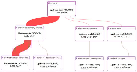
Figure 9.
Process network for VCRM1 scenario for global warming category.
Figure 10 presents an example process network for the IREC1 scenario showing the impact distribution in the category of fossil resource scarcity. The environmental load is dominated by electricity consumption, as in the global warming category; however, within the production stage, the manufacturing of electronic components as well as parts made of ABS and PP stand out, with contributions of 1.5%, 1.2%, and 1.2%, respectively. The relatively high impact of the plastic elements is due to their crude oil origin. Similarly, in the case of the VCRM1 scenario, the production processes of electronic components and ABS parts have the greatest contribution to the total impact of the AC unit production stage (1.2% and 0.8%, respectively), apart from the dominant impact of electricity consumption (96%).
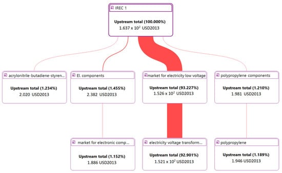
Figure 10.
Process network for IREC1 scenario for fossil resource scarcity category.
As mentioned previously, in the VCRM1 scenario, the COP obtained using Equation (8) amounted to 1.06, which does not seem to reflect actual operation conditions. The greatest discrepancy was observed for low-temperature differences between outdoor and target room air. Thus, it can be concluded that Equation (8) does not provide an appropriate estimation and should be modified to account for the nonlinear impact of the ambient temperature on VCRM AC unit performance. Therefore, another scenario, VCRM2, was developed based on a revised calculation method, assuming specific power consumption for every degree of cooling the specified volumetric flow rate (for maximum 440 m3/h per HMX core). In this case, the COP of the VCRM was adopted at an average level of 5 (that corresponds to values for the best available products on the market). Here, one should notice that, for a small temperature difference between ambient and target room temperature, the COP theoretical value could be significantly higher, but according to the technical characteristics of the VCRM AC unit considered, the minimal power consumption is 470 W (caused by fan power consumption to supply the assigned air flow rate and minimal compressor power supply). This fact causes a considerable decrease in the actual COP value throughout the entire operation period. The resulting sum of electricity consumption for May-Sept (2023–2024) was 1786 kW·h, which is 2.4-times lower than in the VCRM1 baseline scenario.
The relative endpoint results for the IREC1 and VCRM2 scenarios expressed in percentage terms are presented in Figure 11, where 100% indicates the total VCRM2 impact for a given endpoint category. Due to reduced electricity consumption by the VCRM unit, the indicators depicted in the ‘el’ sections of the VCRM2 scenario are significantly lower compared to the baseline conditions (by 2.5-times) though still 35% greater than in the case of IREC1. The total environmental load of the latter also remained lower by 29–36% than in the case of VCRM2. For the production stage (‘unit’ section) and end of life (‘eol’ section), there is no change in the results in relation to the previous comparison illustrated in Figure 8 due to the lack of differences in raw materials used for AC unit manufacturing. However, the improvement in VCRM energy performance resulted in a change in the contribution of individual life cycle stages to the total environmental burden of the VCRM2 scenario. The electricity consumption remained the greatest contributor, with a share of 74–89%, despite its share being smaller than in the baseline scenario. Consequently, the contribution of the production stage increased to 10–26%. An increase was also recorded in the case of the end-of-life impact; nonetheless, its proportion remained at 0.24% or lower. The general conclusion that might be drawn from this comparison is that, despite favorable assumptions made for VCRM2 (), the VCRM1 scenario turned out to have a greater environmental impact than the IREC1 scenario, regardless of the damage category.
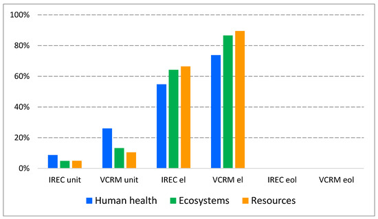
Figure 11.
Relative endpoint indicators for the selected life stages of IREC1 and VCRM2: unit—production stage; el—electricity consumption for operation; eol—end of life.
In order to analyze the environmental impact results more thoroughly, an uncertainty analysis of the input parameters in the LCA model was carried out. For this purpose, a Monte Carlo simulation with 5000 iterations was applied. Among the results obtained, extremely high deviations were observed for the categories related to water consumption (water consumption terrestrial ecosystem, water consumption aquatic ecosystems and water consumption human health). The probable reason is the heterogeneity of regional data for water use and consequent differences in their impact, as determined for various regions, since the impact of water consumption depends strongly on local hydrological conditions and water stress. The differences between the mean values and percentiles (5th and 95th) even reached thousands of percent, particularly for water consumption terrestrial ecosystem. On the other hand, the water consumption categories had relatively small contributions to total endpoint indicators: 0.7% in human health and 2.3–2.4% in ecosystems. Given this, the deviations in the results for the categories of water consumption were neglected, and, instead, the mean values were considered in the uncertainty analysis. Thanks to this approach, the results are clearly displayed in the chart. The confidence intervals for the 5th and 95th percentiles obtained in this way for individual endpoint categories are marked in Figure 12 with vertical lines. The ranges of the indicators confirm the general conclusions that the IREC system has a lower environmental impact than the VCRM system. Even when considering the most optimistic 5th percentile of the VCRM2 scenario, the damage indicators are greater than the mean indicators for the IREC1 scenario, regardless of the impact category.
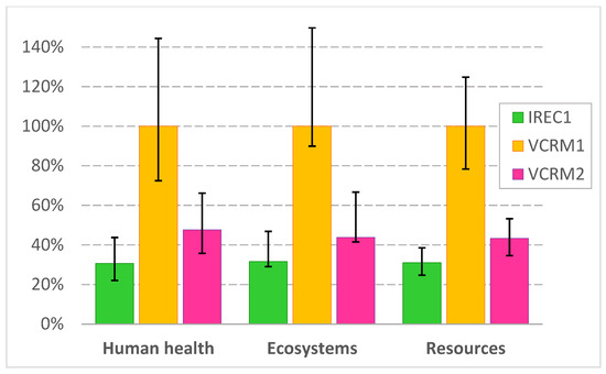
Figure 12.
Relative endpoint indicators of individual scenarios with confidence intervals for 5th and 95th percentiles.
Since, for all considered scenarios, the most relevant contributor to the total environmental impact was associated with electricity consumption necessary for AC unit operation, within the sensitivity analysis, other scenarios were examined under the assumption that the systems are used in a different region. The baseline scenarios as well as the VCRM2 one assumed an electricity mix specific to Ukraine. As an alternative, the European electricity mix was implemented, which is characterized by a significantly higher proportion of renewable energy sources but lower proportion of nuclear energy. The scenarios assuming the European electricity mix were named IRECeur and VCRMeur. Apart from the energy source, there is no difference between them and IREC1 and VCRM2.
The relative endpoint results for the IRECeur and VCRMeur scenarios are presented in Figure 13, where 100% indicates the total VCRMeur impact for a given endpoint category. Due to the change in the electricity mix, the indicators for electricity consumption (‘el’ sections) decreased by 20–24% compared to the IREC1 and VCRM2 scenarios. Despite the resulting impact reduction, the AC systems’ operation stage remained the most relevant, with the contribution to the total environmental load amounting to 83–91% in the case of the IRECeur scenario and 69–87% in the case of the VCRMeur one. Nevertheless, the IREC system demonstrated a lower total environmental burden by 29–38%, depending on the damage category.
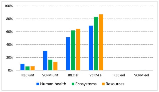
Figure 13.
Relative endpoint indicators for the selected life stages of IRECeur and VCRMeur. unit—production stage; el—electricity consumption for operation; eol—end of life.
4. Conclusions
This study presents a comparative life cycle assessment of an innovative indirect regenerative evaporative cooling (IREC) system compared to a traditional vapor compression refrigeration machine (VCRM) for ducted air conditioning. This study defined the functional unit as a 5 kW capacity system operating during the summer seasons over a 10-year lifespan. The amounts of cooling energy provided and electricity consumption were based on temperature and relative humidity data recorded at hourly intervals in the summer seasons of 2023 and 2024.
The results of the baseline scenarios comparison (IREC1 versus VCRM1) suggest that the IREC system exhibits a substantially lower environmental impact, ranging from 29% to 70% across all endpoint categories. This significant advantage is attributed primarily to the markedly higher seasonal coefficient of performance for the IREC unit, 3.48 compared to 1.06 for the baseline VCRM scenario, which translates into reduced electricity consumption throughout the operational phase, which is the most environmentally burdensome stage. Since the coefficient of performance in the VCRM1 scenario turned out to be unrealistically low, the results of the baseline comparison should not drive recommendations for decision makers. To ensure robustness, a scenario with improved VCRM performance (VCRM2, ) was evaluated. Despite achieving a 2.4-fold reduction in electricity consumption compared to VCRM1, this system still generated endpoint impacts that were 40–57% higher than those of the IREC system. Electricity consumption for system operation remained the most environmentally burdensome stage. Production-related impacts ranked second in significance, contributing 7–26% depending on the system and damage category. The IREC system benefited from a simpler unit design, using fewer and less environmentally impactful materials, which led to a 2.1–3.0-times lower manufacturing burden than the VCRM unit. The end-of-life phase had a negligible environmental impact (<0.3%) for both systems. Notably, the global warming category was the most impactful one, accounting for over 50% of the damage in the human health category and over 75% of the ecosystem damage. Fossil resource scarcity also emerged as the dominant driver in the resources endpoint category, contributing over 98% of total damage.
A Monte Carlo uncertainty analysis revealed extreme variability in water consumption-related categories, with differences between the 5th and 95th percentiles reaching thousands of percent, especially in the water consumption terrestrial ecosystem category. This deviation stems from regional disparities in water scarcity and stress factors within the impact modeling framework. However, as these categories accounted for only 0.7% of damage in human health and 2.3–2.4% in ecosystems, the overall conclusions were unaffected.
Sensitivity analysis showed that switching from the Ukrainian to the European electricity mix led to 20–24% reductions in electricity-related impacts. Nevertheless, the ranking of systems remained unchanged. The IREC system maintained its advantage over both baseline and optimized VCRM scenarios. In the context of the European electricity mix (IRECeur vs. VCRMeur), the IREC system still demonstrated 29–38% lower total damage indicators, depending on the category.
Given all comparisons carried out, this study confirms that IREC systems are not only technically viable but also environmentally advantageous alternatives to traditional vapor compression systems in suitable climates. Their adoption could contribute meaningfully to reducing energy consumption, lowering greenhouse gas emissions, and minimizing life cycle environmental burdens associated with indoor climate control. This advantage results from significantly higher efficiency (COP) in dry and hot climates, which, given the noticeable climate changes, creates an increasingly wider market for the application of this technology. The results obtained can be extrapolated to countries or regions with similar climatic conditions.
However, it should be emphasized that the IREC system is represented by a prototype unit, which is being compared to a technologically mature VCRM unit. Thus, some corresponding risks, such as slight discrepancies in characteristics or operational reliability issues, may occur and, apparently, can be mitigated after the finalization of product development of the IREC AC system by II LLC. On the other hand, vapor compression technology is not significantly affected by ambient humidity and can provide more stable maintenance of the indoor air temperature for the end user. Moreover, vapor compression systems are reversible and can operate in heat pump mode, which allows the same unit to be used for space heating. Considering the above, it can be concluded that for duct air conditioning systems and AHU units, the combination of vapor compression air conditioning systems with IREC technology is highly promising. Such a solution will significantly reduce energy consumption in the summer season, stabilize the indoor parameters under high-humidity conditions, and also provide heating during the off-season and winter.
Author Contributions
Conceptualization, D.L. and A.M.; methodology, D.L. and A.M.; software, D.L. and A.M.; formal analysis, D.L. and A.M.; investigation, D.L. and A.M.; resources, D.L. and A.M.; writing—original draft preparation, D.L. and A.M.; visualization, D.L. and A.M. All authors have read and agreed to the published version of the manuscript.
Funding
This research received no external funding.
Data Availability Statement
Data are contained within the article.
Acknowledgments
The authors express their sincere gratitude to Innovative Ideas LLC and its CEO, Stanislav Shevchenko, for providing the experimental and manufacturing data on the IREC AC unit, which were essential for this research.
Conflicts of Interest
The authors declare no conflicts of interest.
References
- Agostini, B.; Fabbri, M.; Park, J.E.; Wojtan, L.; Thome, J.R.; Michel, B. State of the Art of High Heat Flux Cooling Technologies. Heat Transf. Eng. 2007, 28, 258–281. [Google Scholar] [CrossRef]
- Kumar Sharma, K.; Gupta, R.L.; Katarey, S. Performance Improvement of Air Conditioning System Using Applications of Evaporative Cooling: A Review Paper. Int. J. Therm. Eng. 2016, 2, 1–5. [Google Scholar] [CrossRef]
- IEA Report. Air Conditioning Use Emerges as One of The Key Drivers of Global Electricity-Demand Growth. Available online: https://www.iea.org/news/air-conditioning-use-emerges-as-one-of-the-key-drivers-of-global-electricity-demand-growth (accessed on 30 May 2025).
- Ko, J.; Jeong, J.H. Status and Challenges of Vapor Compression Air Conditioning and Heat Pump Systems for Electric Vehicles. Appl. Energy 2024, 375, 124095. [Google Scholar] [CrossRef]
- Wang, C.; Lei, B.; Zhang, Z.; Liu, Q.; Wu, J. Theoretical Study on the Vapor Compression Cycles with Nearly Isothermal Compression for Various LGWP Refrigerants Using Oil Injection. Appl. Therm. Eng. 2025, 264, 125510. [Google Scholar] [CrossRef]
- Zhang, L.; Jiang, Y.; Dong, J.; Yao, Y. Advances in Vapor Compression Air Source Heat Pump System in Cold Regions: A Review. Renew. Sustain. Energy Rev. 2018, 81, 353–365. [Google Scholar] [CrossRef]
- Rostamzadeh, H.; Rostamzadeh, J.; Matin, P.S.; Ghaebi, H. Novel Dual-Loop Bi-Evaporator Vapor Compression Refrigeration Cycles for Freezing and Air-Conditioning Applications. Appl. Therm. Eng. 2018, 138, 563–582. [Google Scholar] [CrossRef]
- Skye, H.M.; Domanski, P.A.; Brignoli, R.; Lee, S.; Bae, H. Validation of and Optimization with a Vapor Compression Cycle Model Accounting for Refrigerant Thermodynamic and Transport Properties: With Focus on Low-GWP Refrigerants for Air-Conditioning. Int. J. Refrig. 2023, 147, 106–120. [Google Scholar] [CrossRef]
- Subiantoro, A.; Ooi, K.T. Economic Analysis of the Application of Expanders in Medium Scale Air-Conditioners with Conventional Refrigerants, R1234yf and CO2. Int. J. Refrig. 2013, 36, 1472–1482. [Google Scholar] [CrossRef]
- She, X.; Yin, Y.; Zhang, X. A Proposed Subcooling Method for Vapor Compression Refrigeration Cycle Based on Expansion Power Recovery. Int. J. Refrig. 2014, 43, 50–61. [Google Scholar] [CrossRef]
- Miyawaki, K.; Shikazono, N. Experimental Evaluation of NIR Spectroscopic Characteristics of Liquid R32, R1234yf and R454C Refrigerants. Int. Commun. Heat Mass Transf. 2024, 156, 107633. [Google Scholar] [CrossRef]
- Hossain, M.N.; Ghosh, K. A Comparative Study of Plain and Enhanced Helical Microfin Evaporator Tube with Drift Flux-Based Entropy Generation Model for R32 and R410A Refrigerants. Int. J. Heat Mass Transf. 2023, 215, 124441. [Google Scholar] [CrossRef]
- Maeda, S.; Thu, K.; Maruyama, T.; Miyazaki, T. Critical Review on the Developments and Future Aspects of Adsorption Heat Pumps for Automobile Air Conditioning. Appl. Sci. 2018, 8, 2061. [Google Scholar] [CrossRef]
- Islam, M.A.; Mitra, S.; Thu, K.; Saha, B.B. Study on Thermodynamic and Environmental Effects of Vapor Compression Refrigeration System Employing First to Next-Generation Popular Refrigerants. Int. J. Refrig. 2021, 131, 568–580. [Google Scholar] [CrossRef]
- Mtibaa, A.; Sessa, V.; Guerassimoff, G.; Alajarin, S. Refrigerant Leak Detection in Industrial Vapor Compression Refrigeration Systems Using Machine Learning. Int. J. Refrig. 2024, 161, 51–61. [Google Scholar] [CrossRef]
- Lai, L.; Wang, X.; Hu, E.; Choon Ng, K. A Vision of Dew Point Evaporative Cooling: Opportunities and Challenges. Appl. Therm. Eng. 2024, 244, 122683. [Google Scholar] [CrossRef]
- Liu, X.; Jing, C.; Lyu, S. Performance Study of Indirect Perforated Dew-Point Evaporative Coolers. Available online: https://www.researchsquare.com/article/rs-4248663/v1 (accessed on 30 May 2025).
- Khan, I.; Khalid, W.; Ali, H.M.; Sajid, M.; Ali, Z.; Ali, M. An Experimental Investigation on the Novel Hybrid Indirect Direct Evaporative Cooling System. Int. Commun. Heat Mass Transf. 2024, 155, 107503. [Google Scholar] [CrossRef]
- Romero-Lara, M.J.; Comino, F.; Ruiz de Adana, M. Experimental Assessment of the Energy Performance of a Renewable Air-Cooling Unit Based on a Dew-Point Indirect Evaporative Cooler and a Desiccant Wheel. Energy Convers. Manag. 2024, 310, 118486. [Google Scholar] [CrossRef]
- Xiao, X.; Liu, J. A State-of-Art Review of Dew Point Evaporative Cooling Technology and Integrated Applications. Renew. Sustain. Energy Rev. 2024, 191, 114142. [Google Scholar] [CrossRef]
- Sajjad, U.; Abbas, N.; Hamid, K.; Abbas, S.; Hussain, I.; Ammar, S.M.; Sultan, M.; Ali, H.M.; Hussain, M.; Rehman, T.U.; et al. A Review of Recent Advances in Indirect Evaporative Cooling Technology. Int. Commun. Heat Mass Transf. 2021, 122, 105140. [Google Scholar] [CrossRef]
- Zhu, G.; Wen, T.; Wang, Q.; Xu, X. A Review of Dew-Point Evaporative Cooling: Recent Advances and Future Development. Appl. Energy 2022, 312, 118785. [Google Scholar] [CrossRef]
- Kapilan, N.; Isloor, A.M.; Karinka, S. A Comprehensive Review on Evaporative Cooling Systems. Results Eng. 2023, 18, 101059. [Google Scholar] [CrossRef]
- Yang, Y.; Ren, C.; Yang, C.; Tu, M.; Luo, B.; Fu, J. Energy and Exergy Performance Comparison of Conventional, Dew Point and New External-Cooling Indirect Evaporative Coolers. Energy Convers. Manag. 2021, 230, 113824. [Google Scholar] [CrossRef]
- Sohani, A.; Sayyaadi, H.; Mohammadhosseini, N. Comparative Study of the Conventional Types of Heat and Mass Exchangers to Achieve the Best Design of Dew Point Evaporative Coolers at Diverse Climatic Conditions. Energy Convers. Manag. 2018, 158, 327–345. [Google Scholar] [CrossRef]
- Bhat, S.A.; Sajjad, U.; Hussain, I.; Yan, W.M.; Raza, H.M.U.; Ali, H.M.; Sultan, M.; Omar, H.; Azam, M.W.; Bozzoli, F.; et al. Experiments and Modeling on Thermal Performance Evaluation of Standalone and M-Cycle Based Desiccant Air-Conditioning Systems. Energy Rep. 2024, 11, 1445–1454. [Google Scholar] [CrossRef]
- Mahmood, M.H.; Sultan, M.; Miyazaki, T.; Koyama, S.; Maisotsenko, V.S. Overview of the Maisotsenko Cycle—A Way towards Dew Point Evaporative Cooling. Renew. Sustain. Energy Rev. 2016, 66, 537–555. [Google Scholar] [CrossRef]
- Hussain, T. Optimization and Comparative Performance Analysis of Conventional and Desiccant Air Conditioning Systems Regenerated by Two Different Modes for Hot and Humid Climates: Experimental Investigation. Energy Built Environ. 2023, 4, 281–296. [Google Scholar] [CrossRef]
- Pandelidis, D.; Niemierka, E.; Pacak, A.; Jadwiszczak, P.; Cichoń, A.; Drąg, P.; Worek, W.; Cetin, S. Performance Study of a Novel Dew Point Evaporative Cooler in the Climate of Central Europe Using Building Simulation Tools. Build. Environ. 2020, 181, 107101. [Google Scholar] [CrossRef]
- Zhao, H.; Li, Q.; Wang, Z.; Wu, T.; Zhang, M. Synthesis of MIL-101 (Cr) and Its Water Adsorption Performance. Microporous Mesoporous Mater. 2020, 297, 110044. [Google Scholar] [CrossRef]
- Kandeal, A.W.; Joseph, A.; Elsharkawy, M.; Elkadeem, M.R.; Hamada, M.A.; Khalil, A.; Eid Moustapha, M.; Sharshir, S.W. Research Progress on Recent Technologies of Water Harvesting from Atmospheric Air: A Detailed Review. Sustain. Energy Technol. Assess. 2022, 52, 102000. [Google Scholar] [CrossRef]
- Harrouz, J.P.; Katramiz, E.; Ghali, K.; Ouahrani, D.; Ghaddar, N. Life Cycle Assessment of Desiccant—Dew Point Evaporative Cooling Systems with Water Reclamation for Poultry Houses in Hot and Humid Climate. Appl. Therm. Eng. 2022, 210, 118419. [Google Scholar] [CrossRef]
- Tariq, R.; Sheikh, N.A.; Bassam, A.; Xamán, J. Analysis of Maisotsenko Humid Air Bottoming Cycle Employing Mixed Flow Air Saturator. Heat Mass Transf. 2019, 55, 1477–1489. [Google Scholar] [CrossRef]
- Alam, M.S.; Zubir, M.N.B.M.; Muhamad, M.R.; Kazi, S.N.; Öztop, H.F.; Abdullah, S.; Shaikh, K. A Technological Review of Dew Point Evaporative Cooling: Experimental, Analytical, Numerical and Optimization Perspectives. J. Build. Eng. 2024, 91, 109544. [Google Scholar] [CrossRef]
- Khliyeva, O.; Shestopalov, K.; Ierin, V.; Zhelezny, V.; Chen, G.; Neng, G. Environmental and Energy Comparative Analysis of Expediency of Heat-Driven and Electrically-Driven Refrigerators for Air Conditioning Application. Appl. Therm. Eng. 2023, 219, 119533. [Google Scholar] [CrossRef]
- Alberto Huerta-Reynoso, E.; Alfredo López-Aguilar, H.; Alberto Gómez, J.; Guadalupe Gómez-Méndez, M.; Pérez-Hernández, A. Biogas Power Energy Production from a Life Cycle Thinking. In New Frontiers on Life Cycle Assessment-Theory and Application; IntechOpen: London, UK, 2019. [Google Scholar]
- Solano–Olivares, K.; Romero, R.J.; Santoyo, E.; Herrera, I.; Galindo–Luna, Y.R.; Rodríguez–Martínez, A.; Santoyo-Castelazo, E.; Cerezo, J. Life Cycle Assessment of a Solar Absorption Air-Conditioning System. J. Clean. Prod. 2019, 240, 118206. [Google Scholar] [CrossRef]
- ISO 14040; Environmental Management—Life Cycle Assessment—Principles and Framework. International Organization for Standardization: Geneva, Switzerland, 2006.
- ISO 14044; Environmental Management—Life Cycle Assessment—Requirements and Guidelines. International Organization for Standardization: Geneva, Switzerland, 2006.
- Wernet, G.; Bauer, C.; Steubing, B.; Reinhard, J.; Moreno-Ruiz, E.; Weidema, B. The Ecoinvent Database Version 3 (Part I): Overview and Methodology. Int. J. Life Cycle Assess. 2016, 21, 1218–1230. [Google Scholar] [CrossRef]
- Huijbregts, M.A.J.; Steinmann, Z.J.N.; Elshout, P.M.F.; Stam, G.; Verones, F.; Vieira, M.; Zijp, M.; Hollander, A.; van Zelm, R. ReCiPe2016: A Harmonised Life Cycle Impact Assessment Method at Midpoint and Endpoint Level. Int. J. Life Cycle Assess. 2017, 22, 138–147. [Google Scholar] [CrossRef]
- The European FluoroCarbons Technical Committee. Available online: https://www.fluorocarbons.org/news/vdkf-reports-1-12-average-leakage-rates-from-all-plant-types-in-2022/ (accessed on 29 April 2025).
- Shevchenko, S.; Levchenko, D.; Manzharov, A. Innovative Ideas LLC. Available online: https://www.innovativeideas.pro/reports/Report_II_ENG.pdf (accessed on 30 May 2025).
- U4E Energy-Efficient and Climate-Friendly Air Conditioners. 2019. Available online: https://united4efficiency.org/wp-content/uploads/2021/11/U4E_AC_Model-Regulation_EN_2021-11-08.pdf (accessed on 30 May 2025).
- Yumoto, Y.; Ichikawa, T.; Nobe, T.; Kametani, S. Study on Performance Evaluation of a Split Air Conditioning System Under the Actual Conditions. In Proceedings of the International Refrigeration and Air Conditioning Conference, West Lafayette, IN, USA, 10–14 July 2022. Paper 757. [Google Scholar]
- Andrade, Á.; Restrepo, Á.; Tibaquirá, J.E. EER or Fcsp: A Performance Analysis of Fixed and Variable Air Conditioning at Different Cooling Thermal Conditions. Energy Rep. 2021, 7, 537–545. [Google Scholar] [CrossRef]
- Aynur, T.N. Variable Refrigerant Flow Systems: A Review. Energy Build. 2010, 42, 1106–1112. [Google Scholar] [CrossRef]
- Park, Y.C.; Kim, Y.C.; Min, M.K. Performance Analysis on a Multi-Type Inverter Air Conditioner. Energy Convers. Manag. 2001, 42, 1607–1621. [Google Scholar] [CrossRef]
- Meteostat. Available online: https://meteostat.net/en/place/ua/sumy?s=33275&t=2025-03-04/2025-03-11 (accessed on 30 April 2025).
- Choi, K.; Chong, K. Modified Inverse DistanceWeighting Interpolation for Particulate Matter Estimation and Mapping. Atmosphere 2022, 13, 846. [Google Scholar] [CrossRef]
- Attorre, F.; Alfo, M.; De Sanctis, M.; Francesconi, F.; Bruno, F. Comparison of Interpolation Methods for Mapping Climatic and Bioclimatic Variables at Regional Scale. Int. J. Climatol. 2007, 27, 1825–1843. [Google Scholar] [CrossRef]
- Tan, J.; Xie, X.; Zuo, J.; Xing, X.; Liu, B.; Xia, Q.; Zhang, Y. Coupling Random Forest and Inverse Distance Weighting to Generate Climate Surfaces of Precipitation and Temperature with Multiple-Covariates. J. Hydrol. 2021, 598, 126270. [Google Scholar] [CrossRef]
- Wang, H.K.; Chien, C.F. An Inverse-Distance Weighting Genetic Algorithm for Optimizing the Wafer Exposure Pattern for Enhancing OWE for Smart Manufacturing. Appl. Soft Comput. 2020, 94, 106430. [Google Scholar] [CrossRef]
- Cai, J.; Yu, W.; Xu, W.; Wang, K. Research on Air-Conditioning Operation Energy Saving in Internet Data Center. In Proceedings of the 2022 8th International Conference on Hydraulic and Civil Engineering: Deep Space Intelligent Development and Utilization Forum (ICHCE), Xi’an, China, 25–27 November 2022; pp. 1273–1276. [Google Scholar] [CrossRef]
- Liu, F.; Wang, Z.; Zhang, Q. The Application of a Modular Air Conditioning System in Data Center. Procedia Eng. 2017, 205, 2600–2606. [Google Scholar] [CrossRef]
- Amoabeng, K.O.; Opoku, R.; Boahen, S.; Obeng, G.Y. Analysis of Indoor Set-Point Temperature of Split-Type ACs on Thermal Comfort and Energy Savings for Office Buildings in Hot-Humid Climates. Energy Built Environ. 2023, 4, 368–376. [Google Scholar] [CrossRef]
- Almogbel, A.; Alkasmoul, F.; Aldawsari, Z.; Alsulami, J.; Alsuwailem, A. Comparison of Energy Consumption between Non-Inverter and Inverter-Type Air Conditioner in Saudi Arabia. Energy Transit. 2020, 4, 191–197. [Google Scholar] [CrossRef]
- Lim, J.; Yoon, M.S.; Al-Qahtani, T.; Nam, Y. Feasibility Study on Variable-Speed Air Conditioner under Hot Climate Based on Real-Scale Experiment and Energy Simulation. Energies 2019, 12, 1489. [Google Scholar] [CrossRef]
- Wang, N.; Zhang, J.; Xia, X. Energy Consumption of Air Conditioners at Different Temperature Set Points. In Proceedings of the IEEE AFRICON Conference, Victoria Falls, Zambia, 13–15 September 2011. [Google Scholar] [CrossRef]
- Dapito, J.L.; Chua, A.Y. Coefficient of Performance Prediction Model for an On-Site Vapor Compression Refrigeration System Using Artificial Neural Network. Int. J. Technol. 2024, 15, 505–516. [Google Scholar] [CrossRef]
- Belman-Flores, J.M.; Ledesma, S. Statistical Analysis of the Energy Performance of a Refrigeration System Working with R1234yf Using Artificial Neural Networks. Appl. Therm. Eng. 2015, 82, 8–17. [Google Scholar] [CrossRef]
- Viet, D.N.; Pham, H.-L.; Tokura, S.; Nguyen, V.-D.; Nguyen, N.-A.; Lai, N.-A. Study on Power Consumption and Energy Performance of Split-Type Air-Conditioners. J. Sci. Technol. 2014, 100, 31–035. [Google Scholar]
- Setyawan, A.; Najmudin, H.; Badarudin, A.; Sunardi, C. Evaluation of Split-Type Air Conditioner Performance under Constant Outdoor Moisture Content and Varied Dry-Bulb Temperature. Int. J. Heat Technol. 2022, 40, 1277–1286. [Google Scholar] [CrossRef]
- Mitrakusuma, W.H.; Badarudin, A.; Susilawati; Najmudin, H.; Setyawan, A. Performance of Split-Type Air Conditioner under Varied Outdoor Air Temperature at Constant Relative Humidity. J. Adv. Res. Fluid Mech. Therm. Sci. 2022, 90, 42–54. [Google Scholar] [CrossRef]
- Aziz, A.N.; Mahmoud, S.; Al-Dadah, R.; Ismail, M.A.; Almesfer, M.K. Impact of Ambient Temperature and Humidity on the Performance of Vapour Compression Air Conditioning System-Experimental and Numerical Investigation. CFD Lett. 2024, 16, 1–21. [Google Scholar] [CrossRef]
- Wookey, R. Minimum Home Temperature Thresholds for Health in Winter: A Systematic Literature Review; Public Health England: London, UK, 2014.
- Salthammer, T.; Morrison, G.C. Temperature and Indoor Environments. Indoor Air 2022, 32, e13022. [Google Scholar] [CrossRef]
- BS EN 14825:2022; Air Conditioners, Liquid Chilling Packages and Heat Pumps, with Electrically Driven Compressors, for Space Heating and Cooling, Commercial and Process Cooling. Testing and Rating at Part Load Conditions and Calculation of Seasonal Performance. British Standards Institution: London, UK, 2022.
Disclaimer/Publisher’s Note: The statements, opinions and data contained in all publications are solely those of the individual author(s) and contributor(s) and not of MDPI and/or the editor(s). MDPI and/or the editor(s) disclaim responsibility for any injury to people or property resulting from any ideas, methods, instructions or products referred to in the content. |
© 2025 by the authors. Licensee MDPI, Basel, Switzerland. This article is an open access article distributed under the terms and conditions of the Creative Commons Attribution (CC BY) license (https://creativecommons.org/licenses/by/4.0/).