Using Machine Learning and Analytical Modeling to Predict Poly-Crystalline PV Performance in Jordan

Abstract

This study investigates the performance prediction of poly-crystalline photovoltaic (PV) systems in Jordan using experimental data, analytical models, and machine learning approaches. Two 5 kWp grid-connected PV systems at Applied Science Private University in Amman were analyzed: one south-oriented and another east–west (EW)-oriented. Both systems are fixed at an 11° tilt angle. Linear regression, Least Absolute Shrinkage and Selection Operator (LASSO), ElasticNet, and artificial neural networks (ANNs) were employed for performance prediction. Among these, linear regression outperformed the others due to its accuracy, interpretability, and computational efficiency, making it an effective baseline model. LASSO and ElasticNet were also explored for their regularization benefits in managing feature relevance and correlation. ANNs were utilized to capture complex nonlinear relationships, but their performance was limited, likely because of the small sample size and lack of temporal dynamics. Regularization and architecture choices are discussed in this paper. For the EW system, linear regression predicted an annual yield of 1510.45 kWh/kWp with a 2.1% error, compared to 1433.9 kWh/kWp analytically (3.12% error). The south-oriented system achieved 1658.15 kWh/kWp with a 1.5% error, outperforming its analytical estimate of 1772.9 kWh/kWp (7.89% error). Productivity gains for the south-facing system reached 23.64% (analytical), 10.43% (experimental), and 9.77% (predicted). These findings support the technical and economic assessment of poly-crystalline PV deployment in Jordan and regions with similar climatic conditions.

1. Introduction

Achieving net-zero emissions by 2050 is a central objective in mitigating climate change. According to recent global projections, clean energy investment is expected to exceed USD 2 trillion annually by 2030, with solar technologies playing a major role in this transition [1]. Among these, solar photovoltaic (PV) systems have become prominent due to their scalability and continuously decreasing costs. The global installed capacity of PV systems surpassed 1 terawatt (TW) in 2022, with annual additions projected to exceed 200 GW in subsequent years [2].

In Jordan, electricity production has historically depended on imported fossil fuels, making the energy sector vulnerable to geopolitical and price fluctuations. However, the country receives abundant solar radiation ranging between 5 and 7 kWh/m² per day on average, which makes solar energy a strategic option for national energy independence and sustainability [3]. As a result, Jordan has taken steps to develop its solar energy infrastructure, supported by government incentives and international cooperation.

An accurate estimation of PV system output is essential for the planning, design, and operation of solar energy projects. Traditionally, analytical models have been employed for this purpose, utilizing solar geometry, irradiance, and temperature inputs to calculate energy production [4,5,6]. These models often use empirical or semi-empirical formulations and perform well under standard test conditions. However, they typically struggle to account for nonlinear environmental interactions, equipment degradation, and site-specific variability [7,8].

To overcome such limitations, data-driven approaches such as machine learning (ML) have gained increasing attention in solar energy forecasting. ML models can learn from historical data, identify hidden correlations, and offer improved prediction accuracy over purely analytical methods [9,10,11]. These studies [12,13,14] illustrate the gradual shift from traditional empirical and semi-analytical approaches toward hybrid and data-driven techniques. Specifically, Louzazni et al. [12] employed a Nonlinear Auto-Regressive with Exogenous input (NARX) model to forecast PV output using meteorological variables, while their follow-up work [13] enhanced forecasting accuracy by integrating NARX with artificial neural networks and time series decomposition. Similarly, Patel et al. [14] adopted multiple machine learning algorithms including Random Forest and decision tree to predict power generation in a practical small-scale off-grid PV system, emphasizing the real-world utility of data-driven models in resource-constrained settings. However, the integration of ML models with real-world PV performance datasets, especially in data-constrained environments like Jordan, remains underexplored.

Previous studies have applied linear and nonlinear ML methods such as Support Vector Regression, decision trees, and ensemble models to predict PV performance under various climatic conditions [15,16,17,18]. Some works have combined analytical and ML methods to improve robustness and interpretability [19]. Despite these advances, there is still a need for comparative studies that benchmark ML models against analytical models using field-measured data, particularly in Middle Eastern climates with high irradiance variability.

Several recent efforts have explored hybrid modeling frameworks, explainable AI tools, and meta-learning strategies to further enhance forecasting reliability and interpretability in solar energy applications [20,21,22]. These developments reinforce the value of model transparency and generalization, especially for deployment in diverse geographic regions and system configurations.

In this work, we investigate the performance of several regression-based ML models, such as linear regression, LASSO, ElasticNet, and artificial neural networks (ANNs), in predicting the monthly energy output of two poly-crystalline PV systems installed at different orientations (south-facing and east–west-oriented). These predictions are compared to both experimental field measurements and estimates from an analytical model. Our study aims to assess the trade-offs between model complexity, accuracy, and interpretability and to provide a foundation for deploying ML-based forecasting tools in solar energy systems in Jordan and similar regions.

The remainder of this paper is structured as follows: Section 2 introduces the data sources, analytical modeling approach, and ML techniques used. Section 3 presents the results of model comparisons. Section 4 discusses the interpretation of the findings, and Section 5 outlines conclusions and recommendations for future work.

2. Methods

2.1. The Analytical Model of Energy Collection on Poly-Crystalline PV Systems

Jordan lies in a high-solar-insulation band, and its vast solar potential can be exploited to convert solar energy into potable electrical energy using PV systems. In Jordan, the average insulation intensity on a horizontal surface is between 5 and 7 kWh/m²/d. The climate is mid-latitude summer. Its capital city of Amman is located 800 m above sea level, and its angle of latitude is 32°. Jordan has three climatic zones, the largest of which is the desert, which covers around 80% of the country. The western mountain heights, where most of the cities reside, including the capital of Amman, as well as Jordan Valley, which averages around 300 m below sea level, have an entirely different climate than the rest of the country.

Jordan has four distinct seasons: spring and winter are relatively short, while summers are long, dry, and relatively hot. Jordan does not receive the extreme heat that the Gulf countries are accustomed to, and temperatures rarely go over 35 °C even in the peak of summer.

Two types of PV-grid-connected systems working at Applied Science Private University in Amman, Jordan, possessing a power capacity of 5 kWp each, were used in this study. These two PV systems are fixed with a tilt angle of 11° and comprise poly-crystalline south-directed and poly-crystalline EW-oriented systems (which means that half of these PV modules are directed to the east and the other half are directed to the west).

The poly-crystalline solar modules exhibit the following technical characteristics: a rated maximum power of 250 W, a rated voltage of 30.4 V, a rated current of 8.24 A, and an efficiency of 15.6%. The physical dimensions of each module measure 0.99 m by 1.65 m, and a total of 20 panels are utilized. These specifications collectively define the key attributes of each poly-crystalline module.

The productivity of electrical power at the output of the PV modules was measured for three average days for each month of the year, and then their average was found. After that, the average of three days of the month was multiplied by the number of days in each month, and the total sum of energy collection for 12 months was used as the yearly collection of energy for this PV system.

Table 1. A sample of measured electrical power generation at the output of PV modules for the poly-crystalline EW system and metrological data on an average day of the month.

Time	Wind Speed m/s	Air Pressure hPa	Humidity %	Temperature °C	Radiation W/m²	Electric Yield kWh
8:00	0.68	915.4	92.8	6.6	73	0.42
9:00	0.56	915.9	89.7	7.8	116	0.96
10:00	0.64	916.3	81.6	9.3	314	2.28
11:00	0.96	916	74.8	10.1	531	3.74
12:00	0.76	915.3	71.5	10.4	351	3.08
13:00	1.04	914.5	71.1	11	393	3.32
14:00	0.8	913.7	67.1	11.7	465	4.04
15:00	0.84	913	59.9	12.3	355	2.66
16:00	0.96	912.6	56.3	12.9	231	1.06
17:00	0.84	912.2	61	11.3	42	0.26

and

Table 2. A sample of measured electrical power generation at the output of PV modules for the poly-crystalline south-directed system and metrological data on an average day of the month.

Time	Wind Speed m/s	Air Pressure hPa	Humidity %	Temperature °C	Radiation W/m²	Electric Yield kWh
8:00	0.68	915.4	92.8	6.6	73	0.42
9:00	0.56	915.9	89.7	7.8	116	1
10:00	0.64	916.3	81.6	9.3	314	2.58
11:00	0.96	916	74.8	10.1	531	4.54
12:00	0.76	915.3	71.5	10.4	351	3.76
13:00	1.04	914.5	71.1	11	393	3.88
14:00	0.8	913.7	67.1	11.7	465	5.28
15:00	0.84	913	59.9	12.3	355	3.82
16:00	0.96	912.6	56.3	12.9	231	3.44
17:00	0.84	912.2	61	11.3	42	0.86

show a sample of measured electrical power generation at the output of the PV modules for the poly-crystalline south-directed and EW-oriented systems, respectively, as well as metrological data on an average day of the month.

The mathematical expressions used in this work for energy collection at the output of poly-crystalline PV modules are given in [23,24]. Amman is located at an angle of latitude of Φ = 32$°$.

The declination angle, $\mathsf{\delta },$ is expressed as

$$\mathsf{\delta }=23.45\sin \left(360\right[{\displaystyle \frac{\mathbf{284}+\mathbf{n}}{\mathbf{365}}}])$$

(1)

where “n” is the number of days in a year.

The zenith angle $\mathsf{\theta }$z is given by

$$\mathbf{c}\mathbf{o}\mathbf{s}\mathsf{\theta }\mathrm{z}=\cos \mathsf{\Phi }\mathbf{c}\mathbf{o}\mathbf{s}\mathsf{\delta }\mathbf{c}\mathbf{o}\mathbf{s}\mathsf{\omega }+\mathbf{s}\mathbf{i}\mathbf{n}\mathsf{\Phi }\mathbf{s}\mathbf{i}\mathbf{n}\mathsf{\delta }$$

(2)

where “$\mathsf{\omega }$” is the hour angle.

The sunset hour angle “ωs” can be found using the following formula:

$$\mathsf{\omega }\mathrm{s}={\cos }^{-1}(-\tan \mathsf{\delta }\tan \mathsf{\Phi })$$

(3)

The number of daylight hours is

$$\mathbf{N}=(2/15)[{\cos }^{-1}(-\tan \mathsf{\delta }\tan \mathsf{\Phi })]$$

(4)

Atmospheric transmittance for beam radiation “$\mathsf{\tau }$_b” is

$${\mathsf{\tau }}_{\mathrm{b}}={\mathbf{a}}_{\mathbf{o}}+{\mathbf{a}}_{\mathbf{1}}\mathrm{e}-\left({\displaystyle \frac{{\mathbf{K}}_{\mathbf{1}}}{\mathbf{C}\mathbf{o}\mathbf{s}{\mathsf{\theta }}_{\mathbf{z}}}}\right)$$

(5)

where ${\mathbf{a}}_{\mathbf{o}}$, ${\mathbf{a}}_{\mathbf{1}}$, and ${\mathbf{K}}_{\mathbf{1}}$ are standard atmospheric constants and can be found using the following formulas, respectively:

$${\mathbf{a}}_{\mathbf{o}}={\mathbf{r}}_{\mathbf{o}}[0.4237-0.00821]{(\mathbf{6}-\mathbf{A})}^{\mathbf{2}}$$

(6)

$${\mathbf{a}}_{\mathbf{1}}={\mathbf{r}}_{\mathbf{1}}[0.5055+0.00595]{(\mathbf{6.5}-\mathbf{A})}^{\mathbf{2}}$$

(7)

$${\mathbf{k}}_{\mathbf{1}}={\mathbf{r}}_{\mathbf{k}}[0.2711+0.1858]{(\mathbf{2.5}-\mathbf{A})}^{\mathbf{2}}$$

(8)

where “A” is the altitude of the location for Amman in Jordan, which equals 0.8 km. ${\mathbf{r}}_{\mathbf{o}}$, ${\mathbf{r}}_{\mathbf{1}}$, and ${\mathbf{r}}_{\mathbf{k}}$ are the correction factors for certain climate types [24].

Angle of incidence “$\mathsf{\theta }$” is given by

$$\begin{gathered} \mathsf{\theta }={\mathbf{c}\mathbf{o}\mathbf{s}}^{-1}(\sin \mathsf{\delta }\sin \mathsf{\Phi }\cos \mathsf{\beta }-\sin \mathsf{\delta }\cos \mathsf{\Phi }\sin \mathsf{\beta }\cos \mathsf{\gamma }+\cos \mathsf{\delta }\cos \mathsf{\Phi }\cos \mathsf{\beta }\cos \mathsf{\omega }+\cos \mathsf{\delta }\sin \mathsf{\Phi } \\ \sin \mathsf{\beta }\cos \mathsf{\gamma }\cos \mathsf{\omega }+\cos \mathsf{\delta }\sin \mathsf{\beta }\sin \mathsf{\gamma }\sin \mathsf{\omega }) \end{gathered}$$

(9)

The ratio of beam radiation on a tilted surface to that on a horizontal surface ${\mathbf{R}}_{\mathbf{b}}$ is given by

$${\mathbf{R}}_{\mathbf{b}}={\displaystyle \frac{\mathbf{C}\mathbf{o}\mathbf{s}\mathsf{\theta }}{\mathbf{C}\mathbf{o}\mathbf{s}{\mathsf{\theta }}_{\mathbf{z}}}}$$

(10)

The hourly integrated extraterrestrial radiation on a horizontal surface for an hour period in the absence of an atmosphere ${\mathbf{I}}_{\mathbf{o}}$ is

$${\mathbf{I}}_{\mathbf{o}}={\displaystyle \frac{\mathbf{12}\mathbf{\times }\mathbf{3600}\mathbf{\times }\mathbf{G}\mathbf{s}\mathbf{c}}{\mathsf{\pi }}}(1+0.033\cos ({\displaystyle \frac{\mathbf{360}\mathbf{\times }\mathbf{n}}{\mathbf{365}}}))\times [\cos \mathsf{\Phi }\mathbf{c}\mathbf{o}\mathbf{s}\mathsf{\delta }(\sin \mathsf{\omega }2-\sin \mathsf{\omega }1)+(\mathsf{\pi }{\displaystyle \frac{(\mathsf{\omega }\mathbf{2}-\mathsf{\omega }\mathbf{1})}{\mathbf{180}}}\left)\mathbf{s}\mathbf{i}\mathbf{n}\mathsf{\delta }\mathbf{s}\mathbf{i}\mathbf{n}\mathsf{\Phi }\right)]$$

(11)

where Gsc is the solar constant, which equals 1367 W/m², and $\mathsf{\omega }\mathbf{2}\mathrm{and}\mathsf{\omega }\mathbf{1}$ are the upper and lower limits of certain hours of time, respectively.

The hourly extraterrestrial radiation on a tilted surface ${\mathbf{I}}_{\mathbf{o}\mathbf{t}}$ is

$${\mathbf{I}}_{\mathbf{o}\mathbf{t}}={\mathbf{I}}_{\mathbf{o}}\times {\mathbf{R}}_{\mathbf{b}}$$

(12)

The hourly integrated radiation on a tilted surface and on the Earth’s surface in $\mathbf{M}\mathbf{J}/{\mathbf{m}}^{\mathbf{2}}$ is

$$\begin{array}{c}{\mathbf{I}}_{\mathbf{o}\mathbf{t}\mathbf{u}}\hfill \\ {\mathbf{I}}_{\mathbf{o}\mathbf{t}\mathbf{u}}={\mathbf{I}}_{\mathbf{o}\mathbf{t}}\times {\mathsf{\tau }}_{\mathrm{b}}\hfill \end{array}$$

(13)

To convert the units from MJ to WH, we can use the following formula:

1 MJ = 277.77 WH

(14)

The mathematical expressions were calculated for three average days for each month of the year, and then their average was found. After that, the average of three days of the month was multiplied by the number of days in each month, and the total sum of energy collection for 12 months was used as the yearly collection of energy for this PV system.

The analytical and experimental results collected using the data logger and sensors are shown in

Table 3. Monthly experimental and analytical electrical power generation data for poly-crystalline PV systems. Yield values are normalized in kWh/kWp.

	Analytical Generation				Experimental Generation
Month	Poly East–West	Poly East–West	Poly South	Poly South	Poly East–West	Poly East–West	Poly South	Poly South
	(kWh)	(kWh/kWp)	(kWh)	(kWh/kWp)	(kWh)	(kWh/kWp)	(kWh)	(kWh/kWp)
Jan	528.3	101.6	710.8	136.7	299.5	57.6	388.5	74.7
Feb	598.8	115.2	764.8	147.1	474.8	91.3	551.6	106.1
Mar	664.3	127.8	814.8	156.7	728.4	140.1	819.4	157.6
Apr	682.2	131.2	810.7	155.9	743.4	142.9	801.6	154.1
May	663	127.5	775.8	149.2	880.9	169.4	900.9	173.2
Jun	645.1	124.1	750.4	144.3	802.9	154.4	822.8	158.2
Jul	651.8	125.3	760.2	146.2	893.7	171.9	912.7	175.5
Aug	697.3	134.1	815.4	156.8	859.5	165.3	910.8	175.1
Sep	664.8	127.9	808.6	155.5	730.7	140.5	811.6	156.1
Oct	635.4	122.2	797.7	153.4	555.7	106.9	674.9	129.8
Nov	529.9	101.9	718.6	138.2	333.3	64.1	390.2	75.0
Dec	495.6	95.3	619.6	133	386.3	74.3	506.7	97.4
Sum	7456.5	1433.9	9147.4	1772.9	7689.4	1478.7	8491.7	1633.0

.

The yearly collection of electrical energy at the output of two different systems with percentage error is shown in

Table 4. The analytical and experimental yearly electrical power generation.

PV System Type	Analytical Generation	Analytical Generation	Experimental Generation	Experimental Generation	Error
	(kWh)	(kWh/kWp)	(kWh)	(kWh/kWp)
Poly east–west	7456.5	1433.9	7689.4	1478.7	3.12%
Poly south	9147.4	1772.9	8491.7	1633	7.89%

. The percentage error is calculated using the following formula:

$$\mathrm{Error}=\left|{\displaystyle \frac{\mathbf{A}\mathbf{n}\mathbf{a}\mathbf{l}\mathbf{y}\mathbf{t}\mathbf{i}\mathbf{c}\mathbf{a}\mathbf{l}\mathbf{y}\mathbf{e}\mathbf{a}\mathbf{r}\mathbf{l}\mathbf{y}\mathbf{c}\mathbf{o}\mathbf{l}\mathbf{l}\mathbf{e}\mathbf{c}\mathbf{t}\mathbf{i}\mathbf{o}\mathbf{n}-\mathbf{E}\mathbf{x}\mathbf{p}\mathbf{e}\mathbf{r}\mathbf{i}\mathbf{m}\mathbf{e}\mathbf{n}\mathbf{t}\mathbf{a}\mathbf{l}\mathbf{y}\mathbf{e}\mathbf{a}\mathbf{r}\mathbf{l}\mathbf{y}\mathbf{c}\mathbf{o}\mathbf{l}\mathbf{l}\mathbf{e}\mathbf{c}\mathbf{t}\mathbf{i}\mathbf{o}\mathbf{n}}{\mathbf{A}\mathbf{n}\mathbf{a}\mathbf{l}\mathbf{y}\mathbf{t}\mathbf{i}\mathbf{c}\mathbf{a}\mathbf{l}\mathbf{y}\mathbf{e}\mathbf{a}\mathbf{r}\mathbf{l}\mathbf{y}\mathbf{c}\mathbf{o}\mathbf{l}\mathbf{l}\mathbf{e}\mathbf{c}\mathbf{t}\mathbf{i}\mathbf{o}\mathbf{n}}}\right|\times 100\%$$

(15)

From the comparison between analytical and experimental yearly power generation in Table 4, it can be noted that

(1)

In the case of the poly-crystalline EW-directed PV system, the yearly analytical and experimental electrical power generation is 1433.9 and 1478.7 kWh/kWp, respectively, which are in close agreement (the error value equals 3.12%).

(2)

In the case of the poly-crystalline south-directed PV system, the yearly analytical and experimental electrical power generation is 1772.9 and 1633 kWh/kWp, respectively, which are also in close agreement (the error value equals 7.89%).

(3)

The results show that the productivity of the poly-crystalline south-directed PV system is better than that of the EW-directed PV system, with power gains of 23.64 and 10.43% using the analytical and experimental methods, respectively.

2.2. Machine Learning Modeling

2.2.1. Choice of Learning Algorithms

It is a challenge to select the appropriate algorithm for training data. Nevertheless, the clear relationship observed in Figure 1 (see Section 3.1.1) between radiation and electric yield invalidated our initial assumptions regarding the suitability of purely linear models, which rely heavily on linear dependencies. The utilization of ensemble algorithms holds the potential for enhanced performance in theory, as they combine multiple weak learners and may be used in later studies. In this study, the algorithms chosen include linear regression, LASSO, ElasticNet regression, and a neural network model.

Linear regression, regarded as the pioneering form of regression analysis, has been extensively studied and widely applied in practical settings [25]. Its prominence stems from its suitability for models that exhibit linear dependence on unknown parameters, offering a relatively straightforward fitting process compared to nonlinear models. Additionally, the statistical properties of the resulting estimators can be readily determined. When there is only one explanatory variable, it is referred to as simple linear regression, while the scenario involving multiple explanatory variables is known as multiple linear regression. It is essential to differentiate multiple linear regression from multivariate linear regression, which deals with the prediction of multiple correlated dependent variables rather than a single scalar variable [26].

Traditionally, linear regression models are fitted using the least-squares approach, aiming to minimize the squared residuals between observed and predicted data points. However, alternative approaches exist. For instance, least absolute deviation regression minimizes the “lack of fit” using alternative norms. Moreover, a penalized version of the least-squares cost function can be employed, as demonstrated by ridge regression utilizing the L2-norm penalty and lasso regression employing the L1-norm penalty [24,26].

ElasticNet, a widely utilized regularized linear regression technique, combines two popular penalty functions, namely L1 and L2 penalties. To determine the contribution of each penalty, a hyperparameter called alpha (α) is employed, which takes a value between 0 and 1. Alpha assigns the weight for the L1 penalty, while the weight for the L2 penalty is determined as “one minus the alpha,” as depicted in Equation (15) [27,28]:

ElasticNet Penalty = α(L1 Penalty) + (1 − α) (L2 Penalty)

(16)

The advantage of ElasticNet lies in its ability to strike a balance between both penalties, potentially leading to improved performance compared to models that solely employ one of the penalties. Another hyperparameter, lambda (λ), is introduced to control the weight assigned to the sum of both penalties in the loss function, as shown in Equation (16). The default value for lambda is set to 1.0, which applies the fully weighted penalty, while a value of 0 excludes the penalty altogether. It is common to use very small values for lambda, such as 0.001 or smaller [28,29]. ElasticNet tends to perform better when applied to large datasets:

ElasticNet Loss = Loss + λ(ElasticNet Penalty)

(17)

The term “LASSO” represents the acronym for “Least Absolute Shrinkage and Selection Operator,” which is a statistical formula utilized for regularizing data models and feature selection. In comparison to regression methods, it is favored for achieving more accurate predictions. This model implements a shrinkage approach, where data values are pulled closer to a central point, typically the mean. The lasso procedure promotes simplicity by encouraging sparse models with fewer parameters. This type of regression is particularly suitable for models exhibiting high levels of multicollinearity or situations where automating certain aspects of model selection, such as variable selection or parameter elimination, is desired. Lasso regression utilizes the L1 regularization technique and is particularly effective when dealing with a larger number of features, as it automatically handles feature selection [27,30,31].

Artificial neural networks are dynamic information processing systems inspired by the structure and function of the human brain. First proposed by McCulloch and Pitts in 1943, ANNs consist of interconnected processing units that possess self-adapting, self-organizing, and real-time learning capabilities. Over the years, significant progress has been made in research, leading to widespread applications of ANNs since the 1980s. However, this progress has also brought challenges related to network structure and parameter selection, learning sample choice, initial value selection, and the convergence of learning algorithms [32]. The performance of neural networks is closely tied to the number of neurons employed, necessitating a balance between network performance and simplicity to avoid issues such as poor approximation and overfitting. Evolution Algorithms (EAs) have been effectively utilized to optimize the design and parameters of ANNs since the 1990s. Despite the advancements made, computers still fall short in comparison to the human brain’s exceptional abilities in tasks such as facial recognition and speech understanding. The human brain’s learning capability, resilience, and robustness are unmatched, making it a fascinating model for developing neural networks. The interconnected network of neurons, modeled as switches that activate or remain inactive based on weighted inputs, forms the basis of artificial neurons. Networks of these model neurons, known as Perceptrons, were initially limited to solving linearly separable problems, but the development of error back-propagation methods opened the door for solving more complex problems with neural networks [33].

Although this study primarily focused on linear and regularized regression models, we acknowledge the relevance and widespread use of nonlinear machine learning models such as Random Forests, Gradient Boosting Machines (GBM), and Support Vector Regression (SVR) in photovoltaic performance forecasting. These models have demonstrated strong predictive capabilities, particularly in handling complex interactions and nonlinear relationships between features. However, the scope of this work was intentionally framed as a pilot investigation to evaluate the trade-off between interpretability, computational efficiency, and prediction accuracy, especially in data-constrained environments like our test setup.

Linear regression and its variants (LASSO and ElasticNet) were selected due to their transparent behavior and ease of deployment in resource-limited engineering contexts. While artificial neural networks (ANNs) were included to explore nonlinear modeling, their performance was constrained by the dataset’s size and structure. The addition of tree-based ensemble methods or kernel-based algorithms such as SVR could indeed provide enhanced modeling capacity, but often at the cost of reduced interpretability and increased computational complexity.

Nonetheless, we recognize the potential value of incorporating these advanced models. Therefore, we explicitly recommend their integration in future work to enable a more comprehensive comparison across model types. In particular, ensemble models like Random Forest and GBM are well-suited for capturing interactions in tabular data, and SVR is known for its robustness in high-dimensional feature spaces. These models may be especially effective in modeling long-term fluctuations in irradiance and PV yield when combined with historical data patterns, as demonstrated in hybrid ensemble-based frameworks [34].

2.2.2. Performance Measures

It is challenging to select an appropriate performance measure, or evaluation metric, for an ML regression problem. Unlike classification tasks with clear labels, regression involves continuous variables, making it difficult to accurately quantify and assess prediction quality [35,36]. Additionally, data properties, such as distribution, scale, and the presence of outliers, further influence the suitability of a metric. In this work, the following performance measures were used: MSE (Mean Squared Error), RMSE (Root Mean Squared Error), MAE (Mean Absolute Error), and R² (coefficient of determination).

The MSE (Equation (18)) serves as a widely utilized evaluation metric in regression problems. Its computation involves taking the average of the squared discrepancies between predicted and expected target values within a dataset. A lower MSE value suggests that the model’s predictions align more closely with the actual values. While the MSE is well-suited for cases where errors exhibit a normal distribution and the model is expected to produce predictions in proximity to the true values, it may be influenced by outliers. Therefore, it becomes crucial to consider alternative metrics like the MAE to obtain a more comprehensive assessment.

The RMSE (Equation (19)) emerges as a commonly employed evaluation metric for regression tasks. Its computation involves taking the square root of the MSE. The RMSE serves as a gauge of the average magnitude of the discrepancies between predicted and actual values. A lower RMSE value signifies that the model’s predictions are more closely aligned with the actual values. The RMSE possesses several advantages over the MSE. Firstly, the RMSE remains unaffected by the scale of the data, making it a reliable metric for comparing models across diverse datasets. Secondly, the RMSE exhibits greater sensitivity to outliers compared to the MSE, enabling the identification of models that exhibit significant errors on specific data points.

The MAE (Equation (20)) is a widely used evaluation metric in ML, especially in regression tasks. It measures the average absolute difference between predicted and actual values. Unlike the MSE and RMSE, which involve squaring the differences, the MAE directly captures the magnitude of errors without considering their direction. The MAE is more resilient to the influence of outliers since it does not magnify their impact as the MSE and RMSE do. However, compared to the RMSE, the MAE may lack some interpretability as it does not directly indicate the distance between predictions and actual values.

The R-squared (R²) (Equation (21)) evaluation metric is extensively employed in ML to gauge regression model performance. It quantifies the proportion of the variance in the dependent variable that the model captures. R² serves as a measure of the model’s goodness of fit, providing insights into how well it aligns with the observed data in comparison to a baseline model. R² ranges between 0 and 1, where a value of 0 indicates the model’s inability to explain any variance, while a value of 1 represents a perfect fit. However, it is crucial to acknowledge that R² can be misleading when utilized in models with intricate relationships or when the data deviate from the assumptions of linear regression. To obtain a comprehensive evaluation, it is advisable to interpret R² alongside other evaluation metrics and to consider the specific context and limitations of the regression problem at hand. One possible reason for obtaining a low R-squared (R²) value while achieving better results in the MAE, MSE, and RMSE is the presence of nonlinear relationships in the data. R² is a measure of the proportion of variance explained by the model, specifically assuming a linear relationship between the predictors and the response variable. If the underlying relationship is nonlinear, the model’s ability to capture and explain the variance may be limited, leading to a low R² value. On the other hand, the MAE, MSE, and RMSE provide different perspectives on model performance. They directly measure the magnitude or average of errors without explicitly considering the linearity assumption. These metrics are more sensitive to the absolute differences between predicted and actual values and do not depend on the specific shape of the relationship. Therefore, it is possible to have a low R², indicating a weaker linear fit, while observing better results in the MAE, MSE, and RMSE, which capture the accuracy of the predictions in a more general sense. This scenario suggests that the model may be performing well in terms of prediction accuracy or error magnitude, but the linear relationship assumption may not hold strongly, leading to a lower R² value:

$$\mathbf{M}\mathbf{S}\mathbf{E}={\displaystyle \frac{\mathbf{1}}{\mathbf{n}}}{{\sum }_{\mathbf{i}=\mathbf{1}}^{\mathbf{n}}\left({\mathbf{y}}_{\mathbf{i}}-{\hat{\mathbf{y}}}_{\mathbf{i}}\right)}^{\mathbf{2}}$$

(18)

$$\mathbf{RMSE}=\sqrt{{\displaystyle \frac{1}{\mathrm{n}}}{{\sum }_{\mathrm{i}=1}^{\mathrm{n}}\left({\mathrm{y}}_{\mathrm{i}}-{\hat{y}}_{\mathrm{i}}\right)}^2}$$

(19)

$$\mathbf{M}\mathbf{A}\mathbf{E}={\displaystyle \frac{\mathbf{1}}{\mathbf{n}}}{\sum }_{\mathbf{i}=\mathbf{1}}^{\mathbf{n}}\left|{\mathbf{y}}_{\mathbf{i}}-{\hat{\mathbf{y}}}_{\mathbf{i}}\right|$$

(20)

$${\mathrm{R}}^2=\mathbf{1}-{\displaystyle \frac{{{\sum }_{\mathbf{i}=\mathbf{1}}^{\mathbf{n}}\left({\mathbf{y}}_{\mathbf{i}}-{\hat{\mathbf{y}}}_{\mathbf{i}}\right)}^{\mathbf{2}}}{{{\sum }_{\mathbf{i}=\mathbf{1}}^{\mathbf{n}}\left({\mathbf{y}}_{\mathbf{i}}-\stackrel{-}{\mathbf{y}}\right)}^{\mathbf{2}}}}$$

(21)

where $y_i\mathrm{i}\mathrm{s}\mathrm{t}\mathrm{h}\mathrm{e}\mathrm{a}\mathrm{c}\mathrm{t}\mathrm{u}\mathrm{a}\mathrm{l}\mathrm{v}\mathrm{a}\mathrm{l}\mathrm{u}\mathrm{e},{\hat{\mathbf{y}}}_i\mathrm{i}\mathrm{s}\mathrm{t}\mathrm{h}\mathrm{e}\mathrm{p}\mathrm{r}\mathrm{e}\mathrm{d}\mathrm{i}\mathrm{c}\mathrm{t}\mathrm{e}\mathrm{d}\mathrm{v}\mathrm{a}\mathrm{l}\mathrm{u}\mathrm{e},\stackrel{-}{\mathbf{y}}$ is the mean of the observed data, and n is the number of observations.

2.2.3. Model Training and Validation

To ensure a fair and reproducible evaluation of the employed machine learning models, the dataset was partitioned into three subsets: 70% of the data was used for training, 15% for validation, and the remaining 15% for testing. This split enabled an independent evaluation of model performance and reduced the risk of overfitting.

A 5-fold cross-validation strategy was implemented during training for regularized models such as LASSO and ElasticNet. The optimal hyperparameters were determined using grid search. For LASSO regression, the regularization parameter α was tested over the range [0.001, 0.01, 0.1, 1, 10]. For ElasticNet, both α and the mixing ratio λ were varied: α in [0.001, 0.01, 0.1, 1] and λ in [0.1, 0.5, 0.9].

For the artificial neural network (ANN) model, the architecture included one hidden layer with 10 neurons, using the ReLU (Rectified Linear Unit) activation function. The model was trained using the Adam optimizer with a learning rate of 0.001, a batch size of 32, and a maximum of 200 epochs. Early stopping was applied with a patience of 20 epochs to avoid overfitting. The performance was monitored on the validation set, and the best model (with minimum validation loss) was used for final testing.

3. Results

3.1. Machine Learning Predictions of PV Systems

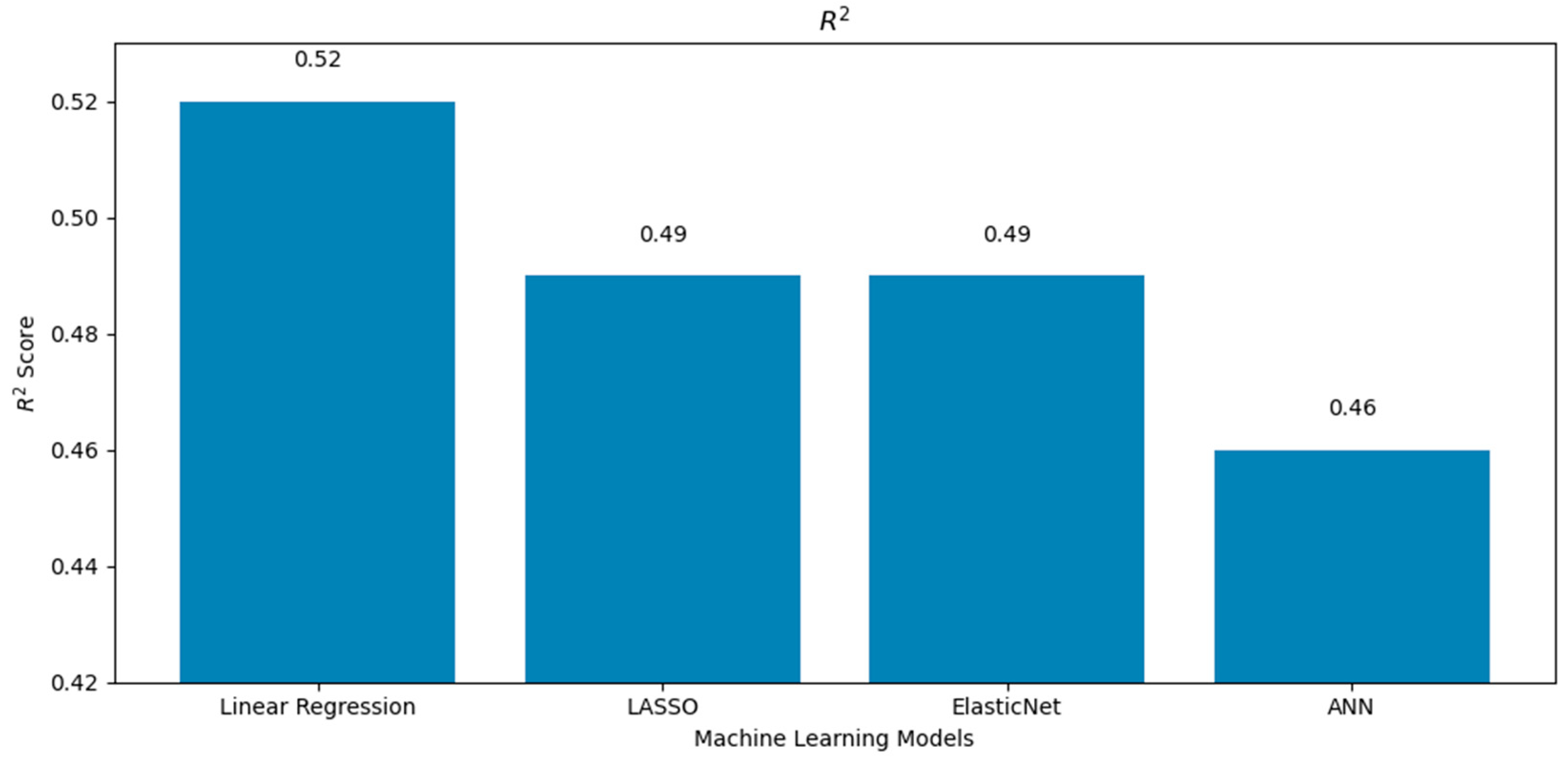
3.1.1. Poly South Predictions

The results in this section are from all the experiments performed on electrical yield and the PV (south and EW) dataset using different ML and deep learning algorithms. In the first part (Section 3.1.1), the poly south system was trained via linear regression, LASSO, and ElasticNet in addition to the ANN algorithms. Figure 1 shows the correlation matrix between the five selected features (wind speed, air pressure, humidity, temperature, and radiation) and the electric power yield at the output of poly-crystalline PV systems. It is shown clearly in Figure 1 that the yield is correlated with the radiation feature. Although radiation shows a strong correlation with energy yield, it was retained in the feature set to preserve the physical interpretability of the models and ensure accurate learning of its interaction with secondary environmental variables. It can also be noted that there is an inverse relationship between humidity and electric power yield. However, other than the other clear correlation between temperature, radiation, and electrical power yield, it can be noted that some features have a very low correlation (i.e., air pressure and wind speed correlation with the other features) and dependency between each other, which may explain the low R².

Figure 2 shows a comparison of the results of the four models (linear regression, LASSO, ElasticNet, and ANN) measured with the evaluation metric MSE on the poly south system.

Figure 2 clearly shows that the linear regression model outperforms the other three models in terms of the MSE. In contrast, the ANN exhibits the weakest performance based on this evaluation metric. Model underperformance is attributed to limited temporal and feature diversity.

Figure 3 shows a comparison of the results of the four models (linear regression, LASSO, ElasticNet, and ANN) measured with the evaluation metric RMSE on the poly south system.

It can be seen clearly in Figure 3 that the linear regression model surpasses all the other three models when measured using the RMSE performance with a value of 1.4525. The ANN underperformed with this evaluation metric as well.

Figure 4 shows a comparison of the results of the four models (linear regression, LASSO, ElasticNet, and ANN) measured with the evaluation metric MAE on the poly south system.

It is shown in Figure 4 that the linear regression model surpasses all the other three models when measured using the MAE performance, at 1.11. However, the ANN underperformed using the MAE evaluation metric, with an MAE score of 1.27.

Figure 5 shows a comparison of the results of the four models (linear regression, LASSO, ElasticNet, and ANN) measured with the evaluation metric R² on the poly south system.

It can be noted in Figure 5 that the linear regression model surpasses all the other three models when measured using the R² performance, at 0.52. The worst performance was for the ANN algorithm with an R² value of 0.46.

While the R² values achieved in this study (0.52 and 0.657 for the best-performing models) appear moderate compared to some other works, this can be attributed to the relatively low variance in the monthly energy yield data collected over a single year. R² is a variance-based metric and tends to be lower when the target variable exhibits limited fluctuation, even if predictions are close to actual values. On the other hand, the percentage errors (2.1% and 1.5%) and MAE metrics directly quantify the deviation from the measured outputs and indicate a strong predictive accuracy. This highlights the importance of using both absolute and relative performance metrics to provide a more complete evaluation of model credibility.

The ANN model used for poly south predictions consisted of a feedforward architecture with one hidden layer comprising 10 neurons. The ReLU activation function was applied in the hidden layer, and a linear activation function was used at the output layer to suit the regression nature of the task.

The model was trained using the Adam optimizer with a learning rate of 0.001. A batch size of 32 and a maximum of 200 epochs were used. To prevent overfitting, early stopping was implemented with a patience of 20 epochs based on validation loss. Additionally, dropout regularization with a rate of 0.2 was employed after the hidden layer.

Despite these strategies, the ANN’s performance lagged behind linear regression and regularized models across all evaluation metrics. The likely cause is the limited size of the dataset and the relatively low temporal granularity, which restricts the ANN’s ability to learn robust nonlinear patterns. Furthermore, the feature set did not include temporal sequences, which often improve neural network performance in forecasting tasks. This limitation is especially critical for ANNs that rely heavily on rich and temporally informative data.

3.1.2. Poly EW Predictions

The results in this section are from all the experiments performed on the electrical yield and PV (EW) dataset using different ML and deep learning algorithms. In this second part, the poly east–west system was trained via linear regression, LASSO, and ElasticNet in addition to ANN algorithms. Figure 6 shows the correlation matrix between the five selected features (wind speed, air pressure, humidity, temperature, and radiation) and the electric power yield. It is observed in Figure 6, like the poly south system, that the yield is clearly correlated with the radiation feature, as explained in Section 3.1.1. It can also be noted that there is an inverse relationship between humidity and electric power yield. However, other than the other clear correlation between temperature, radiation, and electrical power yield, it can be noted that some features have a very low correlation (i.e., air pressure and wind speed correlation with the other features) and dependency between each other, which may explain the low R².

Figure 7 shows a comparison of the results of the four models (linear regression, LASSO, ElasticNet, and ANN) measured with the evaluation metric MSE on the poly east–west system.

Figure 7 clearly shows that the linear regression model outperforms the other three models in terms of the MSE. In contrast, the ANN exhibits the weakest performance based on this evaluation metric. Model underperformance is attributed to limited temporal and feature diversity.

Figure 8 shows a comparison of the results of the four models (linear regression, LASSO, ElasticNet, and ANN) measured with the evaluation metric RMSE on the poly east–west system.

It can be seen clearly in Figure 8 that the linear regression model surpasses all the other three models when measured using the RMSE performance, with a value of 1.09. The ANN underperformed with this evaluation metric as well.

Figure 9 shows a comparison of the results of the four models (linear regression, LASSO, ElasticNet, and ANN) measured with the evaluation metric MAE on the poly east–west system.

It can be noted in Figure 9 that for the first time, the performance of linear regression and the ANN model is almost equivalent and surpasses the other two models when measured using the MAE performance with a value of 0.81 for both. However, the weakest performance for an algorithm using the MAE evaluation metric for the poly east–west system was ElasticNet with an MAE score of 0.83.

Figure 10 shows a comparison of the results of the four models (linear regression, LASSO, ElasticNet, and ANN) measured with the evaluation metric R² on the poly east–west system.

It can be seen clearly in Figure 10 that the linear regression model surpasses all the other three models when measured using the R² performance for the poly east–west system with a value of 0.66. The ANN algorithm underperformed with an R² value of 0.64.

Similar to the poly south case, the ANN model applied to the poly east–west dataset used a single hidden layer with 10 neurons and ReLU activation. Dropout and early stopping were again employed to improve generalization and prevent overfitting.

The ANN model yielded slightly improved results in terms of the MAE when compared to its performance in the poly south system, but still underperformed relative to linear models. This reinforces the observation that in datasets with dominant linear relationships (as shown by the strong correlation between radiation and yield), simpler models tend to generalize better. Additionally, without incorporating temporal patterns or additional exogenous variables (e.g., cloud cover and solar position indices), ANNs are unlikely to outperform well-tuned linear models in this context.

Future research could explore more sophisticated architectures, such as recurrent neural networks (RNNs), gated recurrent units (GRUs), or convolutional neural networks (CNNs), especially when working with time series data or image-based weather predictors. These approaches may help better capture dynamic and nonlinear dependencies present in real-world PV system performance.

4. Discussion

A comparison between monthly analytical, experimental, and predicted electrical power generation by linear regression is shown in

Table 5. The monthly analytical, experimental, and predicted electrical power generation by linear regression.

	Analytical Generation				Experimental Generation				Prediction by Linear Regression Generation
Month	Poly East–West	Poly East–West	Poly South	Poly South	Poly East–West	Poly East–West	Poly South	Poly South	Poly East–West	Poly East–West	Poly South	Poly South
	(kWh)	(kWh/kWp)	(kWh)	(kWh/kWp)	(kWh)	(kWh/kWp)	(kWh)	(kWh/kWp)	(kWh)	(kWh/kWp)	(kWh)	(kWh/kWp)
Jan	528.3	101.6	710.8	136.7	299.5	57.6	388.5	74.7	268.8	51.7	332.3	63.9
Feb	598.8	115.2	764.8	147.1	474.8	91.3	551.6	106.1	350.2	67.4	365.9	70.4
Mar	664.3	127.8	814.8	156.7	728.4	140.1	819.4	157.6	668.2	128.5	763.6	146.9
Apr	682.2	131.2	810.7	155.9	743.4	142.9	801.6	154.1	868.6	167.0	973.	187.1
May	663	127.5	775.8	149.2	880.9	169.4	900.9	173.2	826.7	158.9	894.1	171.9
Jun	645.1	124.1	750.4	144.3	802.9	154.4	822.8	158.2	975.5	187.6	1059.3	203.7
Jul	651.8	125.3	760.2	146.2	893.7	171.9	912.7	175.5	844.9	162.5	845.2	162.5
Aug	697.3	134.1	815.4	156.8	859.5	165.3	910.8	175.1	889.9	171.2	938.5	180.5
Sep	664.8	127.9	808.6	155.5	730.7	140.5	811.6	156.1	777.3	149.5	872.9	167.9
Oct	635.4	122.2	797.7	153.4	555.7	106.9	674.9	129.8	626.3	120.5	710.8	136.7
Nov	529.9	101.9	718.6	138.2	333.3	64.1	390.2	75.0	359.7	69.2	397.4	76.4
Dec	495.6	95.3	619.6	133	386.3	74.3	506.7	97.4	397.9	76.5	469.1	90.2
sum	7456.5	1433.9	9147.4	1772.9	7689.4	1478.7	8491.7	1633.0	7854.3	1510.5	8622.3	1658.2

.

A comparison between yearly analytical, experimental, and predicted electrical power generation by linear regression is shown in

Table 6. The yearly experimental electrical power generation and that predicted by linear regression.

PV System Type	Experimental Generation	Generation Predicted by Linear Regression	Error
	(kWh/kWp)	(kWh/kWp)
Poly east–west	1478.7	1510.45	2.1%
Poly south	1633	1658.15	1.5%

.

The larger discrepancies observed between the analytical, experimental, and predicted values in certain months, particularly during winter periods such as January, February, and December, can be attributed to a combination of environmental and methodological factors. One key contributor is the seasonal variation in sensor accuracy. Temperature fluctuations, increased humidity, and potential condensation can affect sensor stability and response, especially in the absence of regular recalibration. Additionally, winter months in Amman are typically characterized by greater cloud cover and unpredictable atmospheric changes, leading to rapid fluctuations in solar irradiance. These transient effects are not easily captured either by the analytical model, which is based on steady-state solar geometry and average radiation assumptions, or by machine learning models trained on data averaged over longer timeframes.

The analytical model in particular lacks responsiveness to real-time anomalies such as short-term shading, dust accumulation, or precipitation events. On the other hand, while the linear regression model demonstrated a strong overall performance, its predictive accuracy may decline during months with conditions that were underrepresented in the training dataset. These observations highlight the importance of incorporating temporal and exogenous features into future models.

To better represent uncertainty and variation, we recommend the inclusion of statistical measures such as confidence intervals or error bars in future visualizations of both experimental and predicted values. This would allow for a more transparent interpretation of deviations and support data-driven decision making. Expanding the data collection protocol to include auxiliary weather data (e.g., sky imagery or cloud index values) and implementing periodic sensor recalibration could help reduce the unexplained variability and improve both model accuracy and interpretability in future studies.

To further explore the contribution of different environmental features to electrical yield, we trained a Random Forest Regressor and extracted the feature importance scores for the poly EW system (Figure 11). The results clearly indicate that global radiation is the most dominant factor, contributing nearly 80% of the model’s predictive power. In contrast, other meteorological variables such as temperature, humidity, wind speed, and air pressure play relatively minor roles. This aligns with physical expectations, as solar irradiance is the direct energy source driving photovoltaic output. These insights also validate the use of irradiance-focused predictors in lightweight models. However, the inclusion of secondary factors may still aid in refining residual variations, especially in hybrid models. These findings align well with the results of a previous study by Qiu et al. [37], which highlight the central role of irradiance in solar prediction models.

A similar feature importance analysis was conducted for the poly south system, which yielded results closely aligned with those of the poly EW system. Global radiation remained the overwhelmingly dominant factor, while other environmental variables contributed marginally. To avoid redundancy, the feature importance plot for poly south is not shown.

Another limitation of this study is the absence of cloud-related variables in the dataset, which restricts the model’s ability to capture short-term irradiance fluctuations caused by cloud cover. These transient atmospheric changes significantly affect the solar radiation received by PV panels, particularly in winter and during partly cloudy conditions, leading to prediction deviations that are not explained by the current set of features. The lack of sky imagery, satellite data, or real-time cloud indices in our sensor setup limits the model’s responsiveness to such rapid changes in solar availability.

Incorporating cloud cover metrics, whether through satellite-based observations, ground-based sky cameras, or derived Global Horizontal Irradiance (GHI) decomposition, could provide additional predictive value and improve model robustness in future work. Studies utilizing all-sky imaging techniques and time-sequenced irradiance patterns have shown marked improvements in ultra-short-term solar forecasting. For instance, the work by Zuo et al. [38] demonstrated that combining sky image data with historical sequences significantly enhanced GHI prediction accuracy. We acknowledge that integrating such data sources would likely enhance the performance of both machine learning and analytical models and represents a meaningful direction for future extensions of this study.

5. Conclusions and Future Work

In this work, different prediction models of poly-crystalline PV performance in Jordan are studied, including experimental (using a statistical calculation of experimental data), analytical (using mathematical expressions), and ML methods (using four different ML techniques—linear regression, LASSO, ElasticNet, and ANN algorithms). Two types of PV grid-connected systems working at Applied Science Private University in Amman, Jordan, with a power capacity of 5 kWp each, were used in this study. These two PV systems are fixed with a tilt angle of 11° and are poly-crystalline south-directed and poly-crystalline EW-oriented (which means that half of these PV modules are directed to the east and the other half are directed to the west). The linear regression model outperforms the analytical model and all the other three models when compared using different performance measures.

From the comparison between yearly power generation predicted by linear regression, analytical yearly power generation, and experimental yearly power generation in Table 6, it can be noted that

• In the case of the poly-crystalline EW-directed PV system, the yearly analytical electrical power generation is 1433.9 kWh/kWp, where the error value is 3.12% as compared with the experimental value. The yearly electrical power generation predicted by linear regression is 1510.45 kWh/kWp, where the error value is 2.1% as compared with the experimental value. It is seen that the prediction of experimental data by linear regression is very accurate, with an accuracy better than that of the analytical method.
• In the case of the poly-crystalline south-directed PV system, the yearly analytical electrical power generation is 1772.9 kWh/kWp, where the error value is 7.89% as compared with the experimental value. For prediction by linear regression, the yearly electrical power generation is 1658.15 kWh/kWp, where the error value is 1.5% as compared with the experimental value. It can also be noted here that the prediction of experimental data by linear regression is very accurate, with an accuracy better than that of the analytical method.
• The results show that the productivity of the poly-crystalline south-directed PV system is better than that of the poly-crystalline EW-directed PV system, with power gains of 23.64% using the analytical method, 10.43% using the experimental method, and 9.77% using prediction by linear regression.
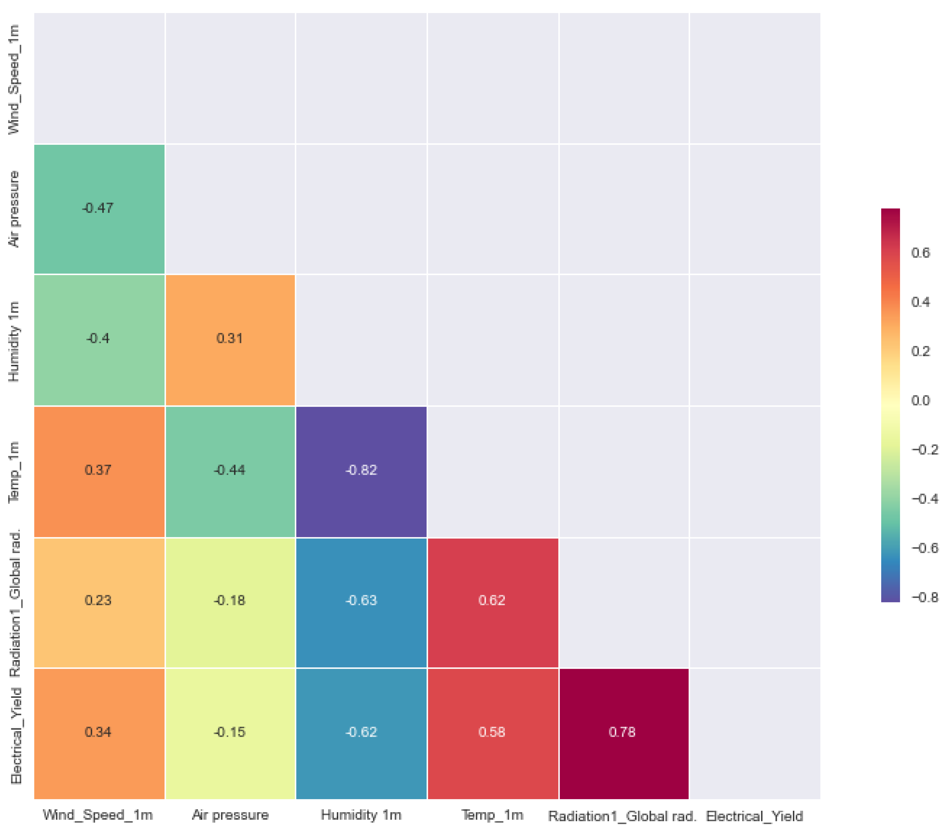
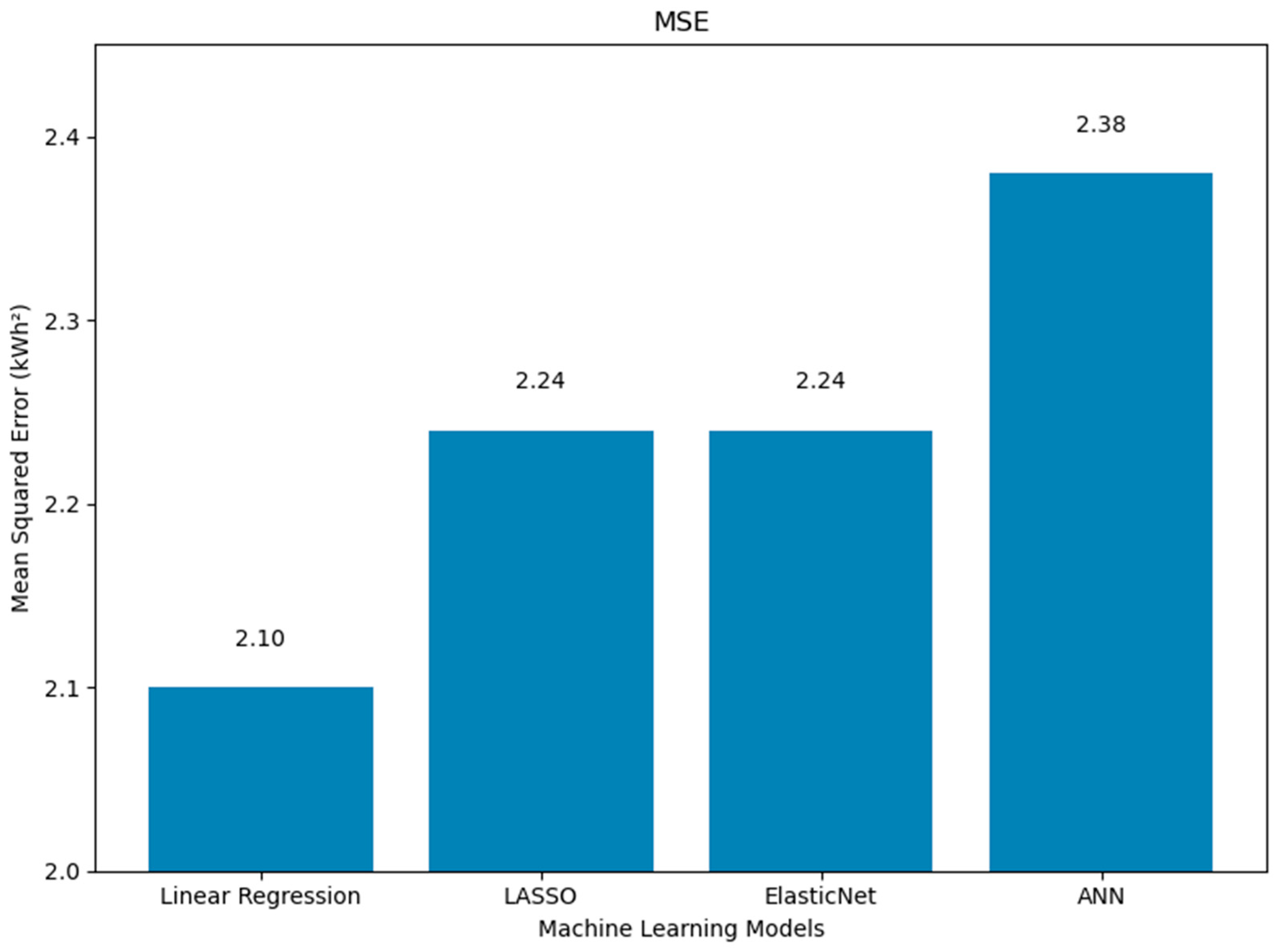
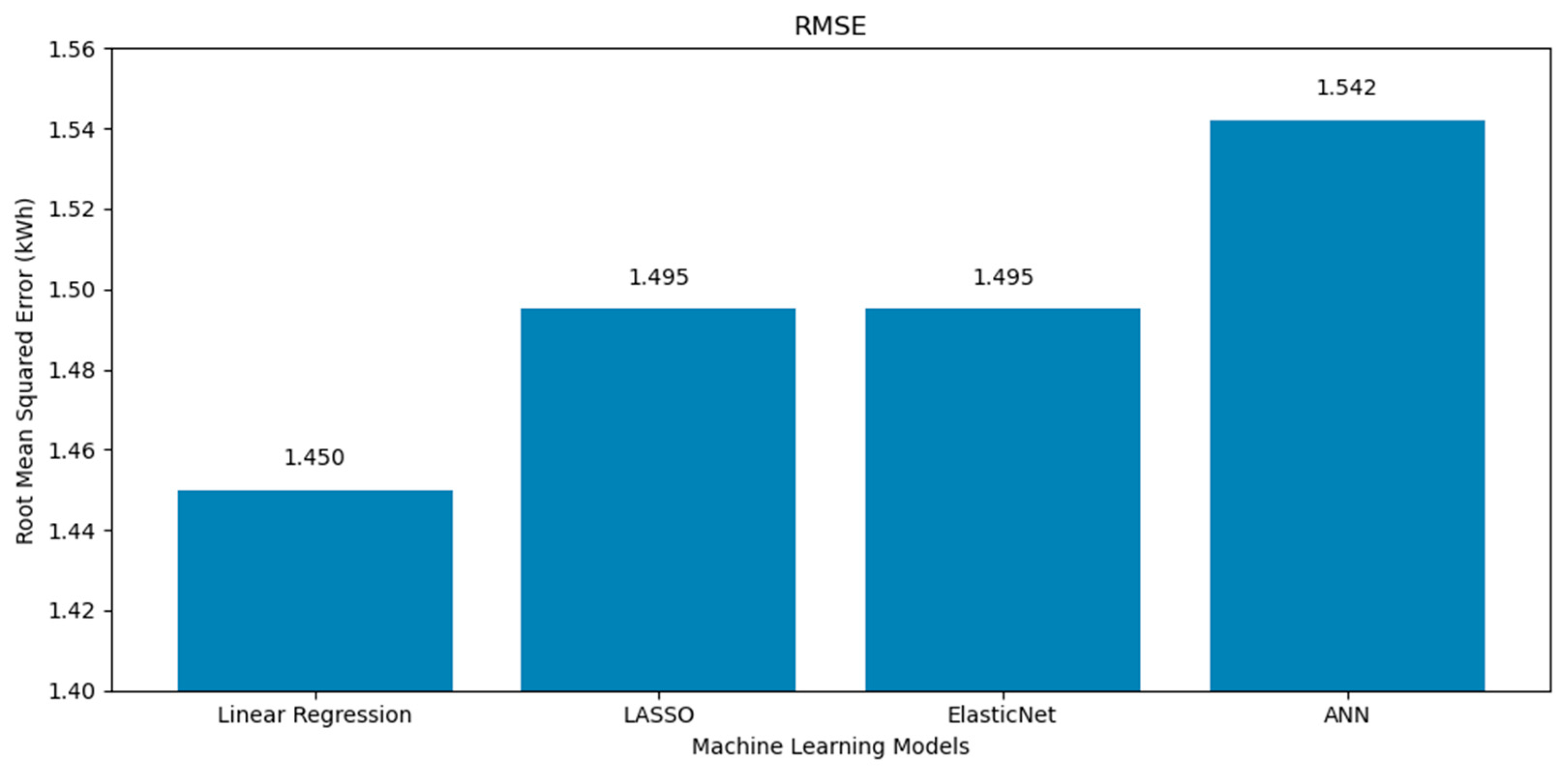
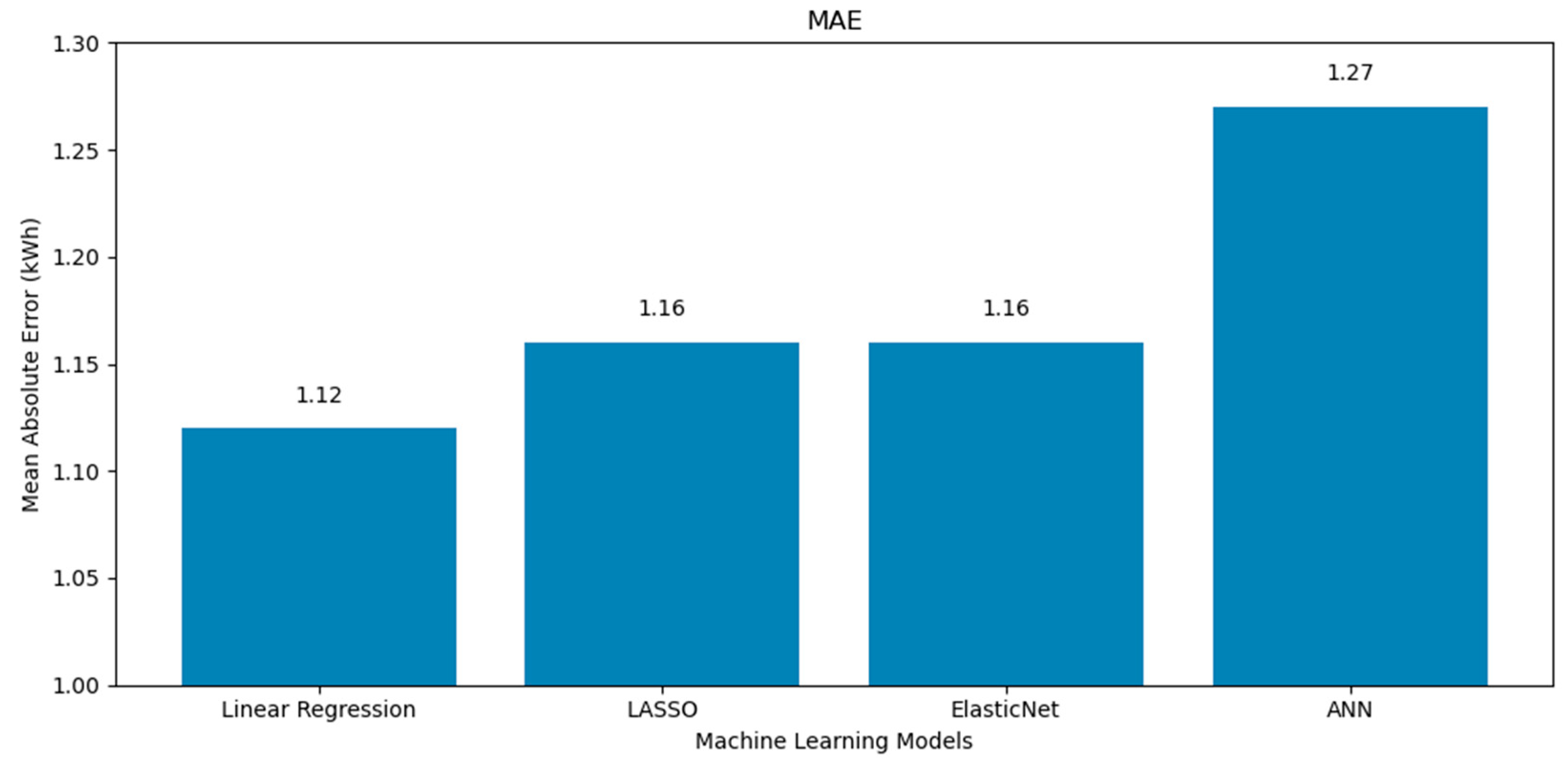
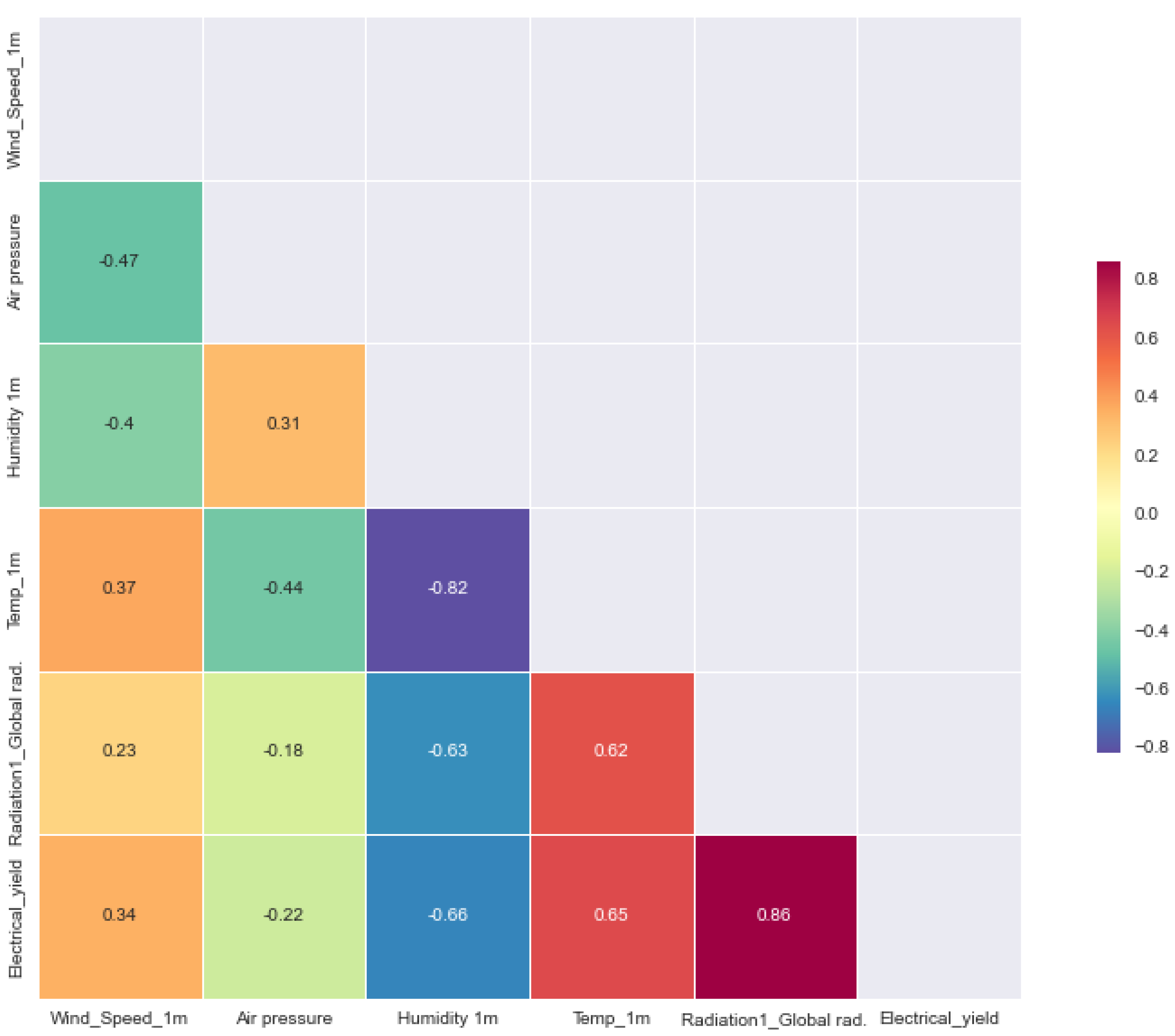
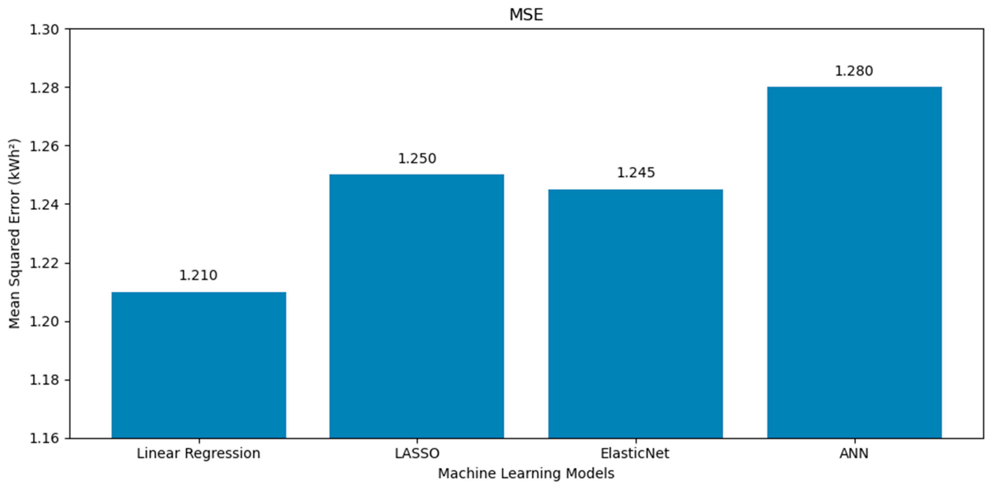
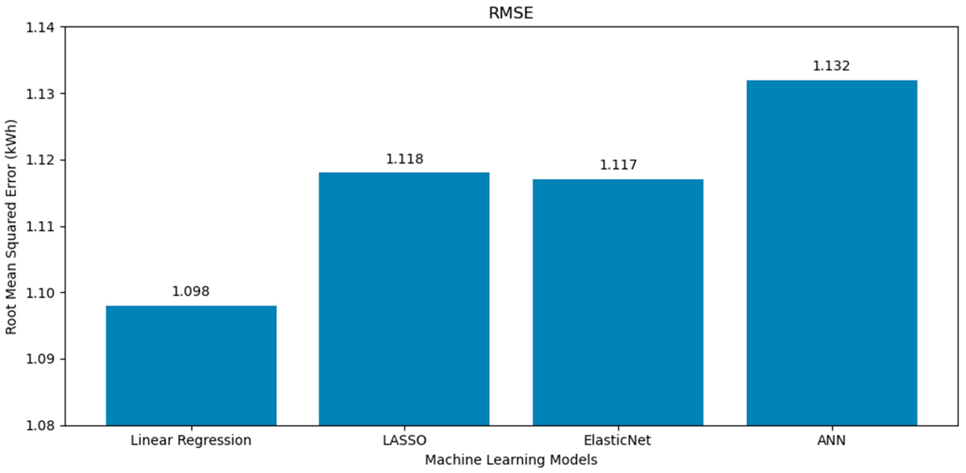
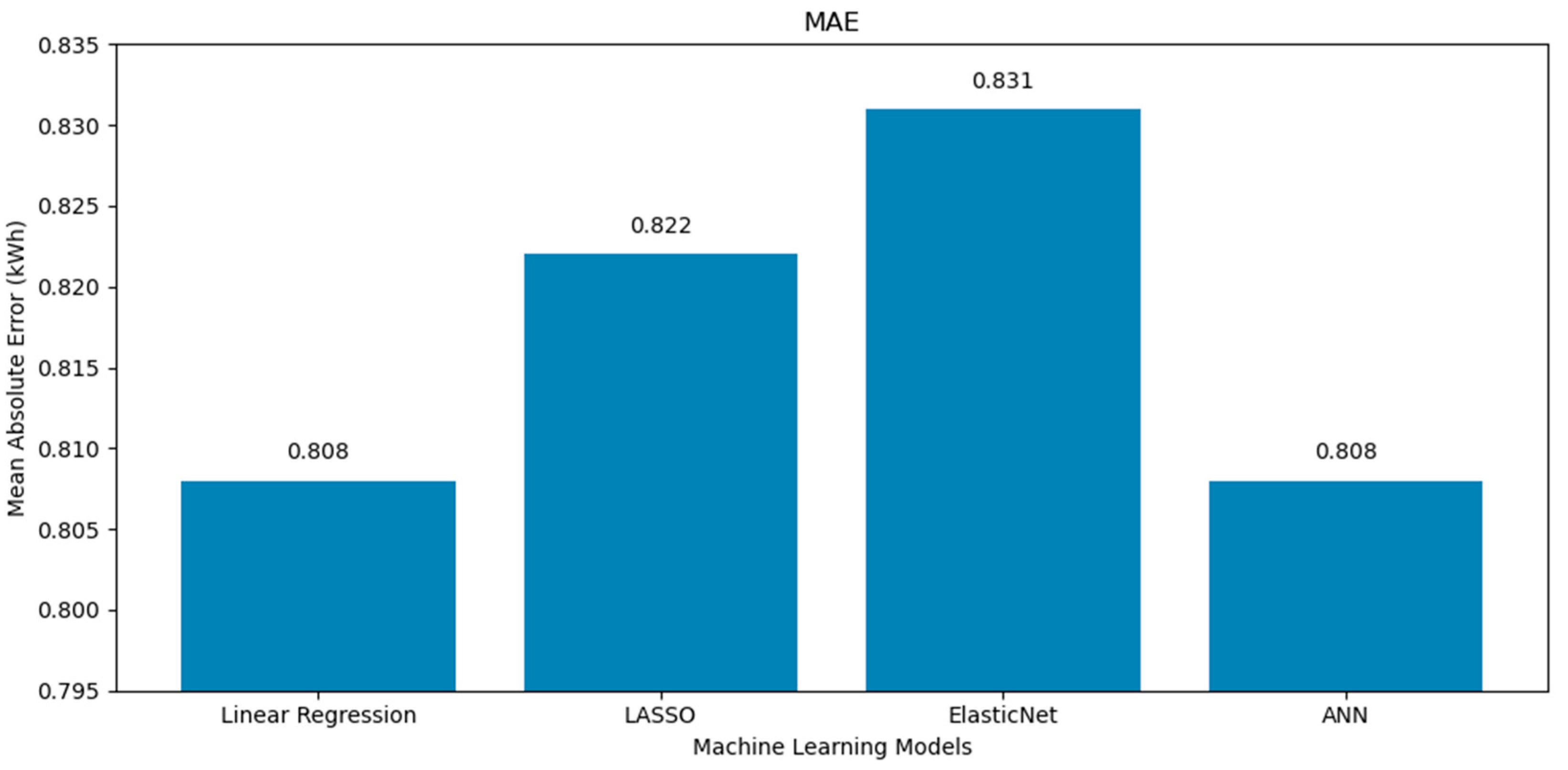
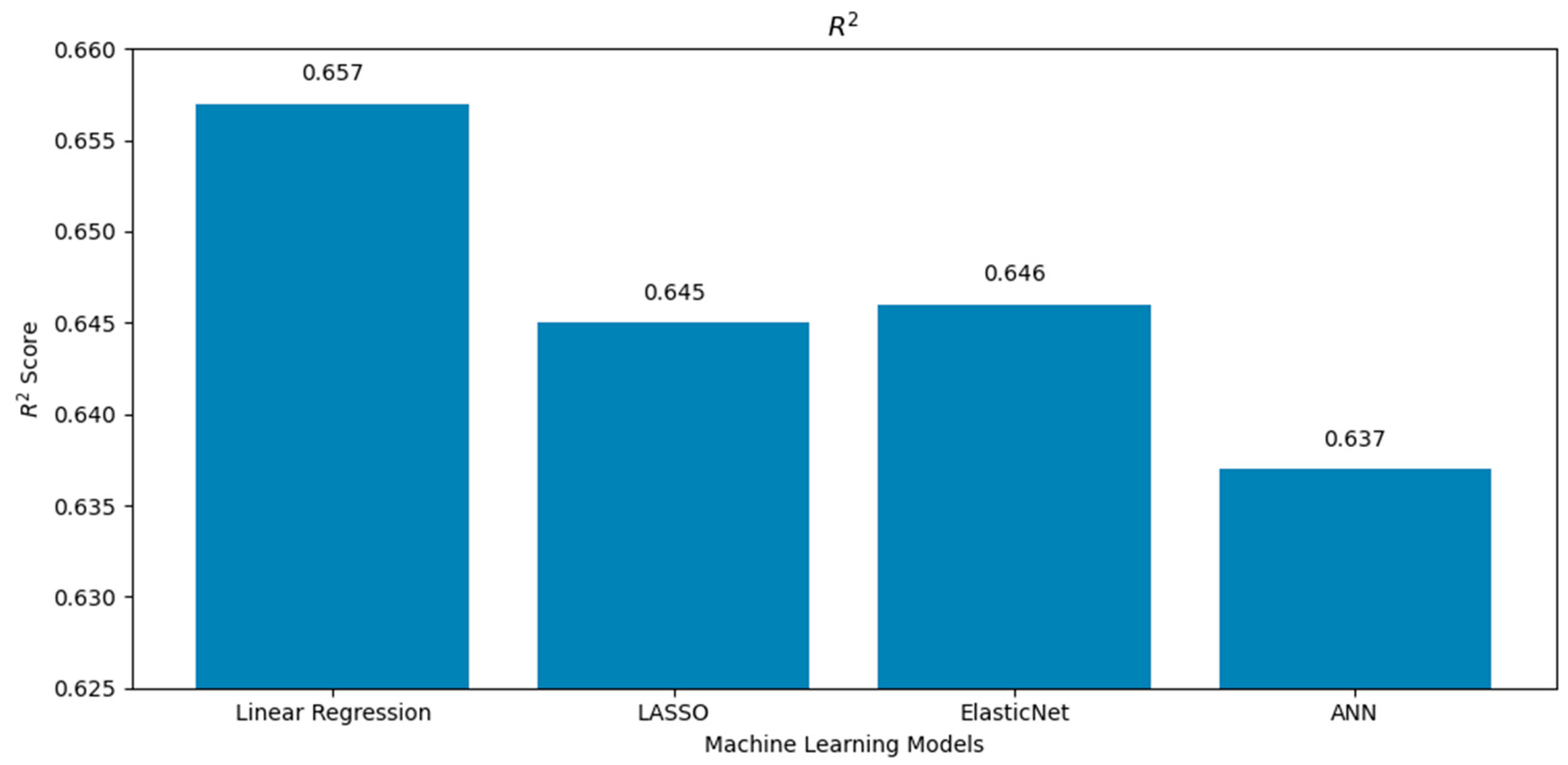
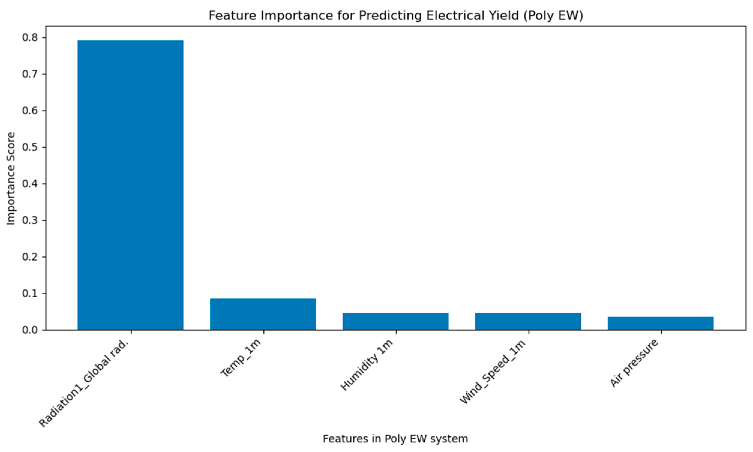
• The superior performance of the linear regression model across all evaluation metrics (the MSE, RMSE, MAE, and R²) in both the poly south and poly EW PV systems can be attributed to several factors. First, the dataset revealed a dominant linear relationship between solar radiation and power yield, as shown in the correlation matrices (Figure 1 and Figure 6), where radiation exhibited the highest positive correlation with output energy. Given that linear regression thrives in contexts where the dependent variable has a strong, linear association with one or more independent variables, this direct relationship likely enabled the model to achieve high predictive accuracy with minimal complexity. By contrast, more complex models such as LASSO, ElasticNet, and ANNs incorporate regularization or nonlinearity, which, while powerful in high-dimensional or noisy environments, can lead to overfitting or underfitting when the underlying patterns are inherently simple. Moreover, the relative sparsity of the features’ interdependence and the limited presence of strong nonlinear interactions further reduced the advantage of using advanced models. Linear regression, with advantages of simplicity and interpretability, was able to generalize well to the test data, yielding error rates even lower than the analytical model and closely matching experimental values, with yearly prediction errors as low as 1.5 and 2.1% for the south and EW systems, respectively. These findings emphasize that in certain practical scenarios with clean, well-structured datasets and dominant linear features, classical statistical methods can outperform more sophisticated machine learning models.

This work focused on comparing analytical, experimental, and machine learning methods for predicting poly-crystalline PV output under clear-sky and general ambient conditions, but it did not incorporate cloud-related variables due to the limitations of our measurement infrastructure. As a direction for future research, we recommend enhancing the feature set by including sky imagery, cloud indices, or satellite-derived GHI decomposition, which could capture short-term irradiance fluctuations more accurately. The integration of such exogenous variables, particularly in combination with advanced time-series or deep learning models, holds promise for significantly improving the precision and reliability of PV performance predictions under dynamic weather conditions.

The results of this study help the installers of PV systems predict the yearly electrical power generation at the output of poly-crystalline PV systems in this region. These results can be used for the technical and economical evaluation of the application of different types of PV systems, and for preparing feasibility studies in Jordan and countries with similar climatic conditions.

References

1. International Energy Agency. World Energy Outlook 2022; IEA: Paris, France, 2022; Available online: https://www.iea.org/reports/world-energy-outlook-2024/executive-summary (accessed on 22 May 2025).
2. Solar Power Europe. Global Market Outlook for Photovoltaics 2022–2026; SolarPower Europe: Brussels, Belgium, 2022. Available online: https://www.memr.gov.jo/EBV4.0/Root_Storage/EN/EB_Info_Page/Summery_of_the_Comprehensive_Strategy_of_the_Energy_Sector_2020_2030.pdf (accessed on 22 May 2025).
3. SolarQuarter. The Future Looks Bright for Solar Energy in Jordan: A 2023 Outlook. Available online: https://solarquarter.com/2023/02/25/the-future-looks-bright-for-solar-energy-in-jordan-a-2023-outlook/ (accessed on 22 May 2025).
4. Ministry of Energy and Mineral Resources. Summary of Jordan Energy Strategy 2020–2030; MEMR: Amman, Jordan, 2022. Available online: https://www.memr.gov.jo/EN/Pages/_Strategic_Plan_ (accessed on 10 April 2025).
5. Tina, G.M.; Ventura, C.; Ferlito, S.; De Vito, S. A State-of-Art Review on Machine-Learning-Based Methods for PV. Appl. Sci. 2021, 11, 7550. [Google Scholar] [CrossRef]
6. Akhter, M.N.; Mekhilef, S.; Mokhlis, H.; Shah, N.M. Review on Forecasting of Photovoltaic Power Generation Based on Machine Learning and Metaheuristic Techniques. IET Renew. Power Gener. 2019, 13, 1009–1023. [Google Scholar] [CrossRef]
7. Zhaoxuan, S.M.; Rahman, M.; Vega, R.; Dong, B. A Hierarchical Approach Using Machine Learning Methods in Solar Photovoltaic Energy Production Forecasting. Energies 2016, 9, 55. [Google Scholar] [CrossRef]
8. Van Tai, D. Solar Photovoltaic Power Output Forecasting Using Machine Learning Technique. J. Phys. Conf. Ser. 2019, 1327, 012051. [Google Scholar] [CrossRef]
9. Nageem, R.; Jayabarathi, R. Predicting the Power Output of a Grid-Connected Solar Panel Using Multi-Input Support Vector Regression. Procedia Comput. Sci. 2017, 115, 723–730. [Google Scholar] [CrossRef]
10. AlKandari, M.; Ahmad, I. Solar Power Generation Forecasting Using Ensemble Approach Based on Deep Learning and Statistical Methods. Appl. Comput. Inform. 2019, 20, 231–250. [Google Scholar] [CrossRef]
11. Anuradha, K.; Erlapally, D.; Karuna, G.; Srilakshmi, V.; Adilakshmi, K. Analysis of Solar Power Generation Forecasting Using Machine Learning Techniques. E3S Web Conf. 2021, 309, 01163. [Google Scholar] [CrossRef]
12. Louzazni, M.; Mosalam, H.; Khouya, A.; Amechnoue, K. A Non-Linear Auto-Regressive Exogenous Method to Forecast the Photovoltaic Power Output. Sustain. Energy Technol. Assess. 2020, 38, 100670. [Google Scholar] [CrossRef]
13. Louzazni, M.; Mosalam, H.; Cotfas, D.T. Forecasting of Photovoltaic Power by Means of Non-Linear Auto-Regressive Exogenous Artificial Neural Network and Time Series Analysis. Electronics 2021, 10, 1953. [Google Scholar] [CrossRef]
14. Patel, A.; Swathika, O.V.G.; Subramaniam, U.; Babu, T.S.; Tripathi, A.; Nag, S.; Karthick, A.; Muhibbullah, M. Practical Approach for Predicting Power in a Small-Scale Off-Grid Photovoltaic System Using Machine Learning Algorithms. Int. J. Photoenergy 2022, 2022, 9194537. [Google Scholar] [CrossRef]
15. Yadav, O.; Kannan, R.; Meraj, S.T.; Masaoud, A. Machine Learning Based Prediction of Output PV Power in India and Malaysia with the Use of Statistical Regression. Math. Probl. Eng. 2022, 2022, 5680635. [Google Scholar] [CrossRef]
16. Khandakar, A.; Chowdhury, M.E.H.; Kazi, M.K.; Benhmed, K.; Touati, F.; Al-Hitmi, M.; Gonzales, A.J.S.P. Machine Learning Based Photovoltaics (PV) Power Prediction Using Different Environmental Parameters of Qatar. Energies 2019, 12, 2782. [Google Scholar] [CrossRef]
17. Kumar, B.S.; Mahilraj, J.; Chaurasia, R.K.; Dalai, C.; Seikh, A.H.; Mohammed, S.M.A.K.; Subbiah, R.; Diriba, A. Prediction of Photovoltaic Power by ANN Based on Various Environmental Factors in India. Int. J. Photoenergy 2022, 2022, 4905980. [Google Scholar]
18. Berghout, T.; Benbouzid, M.; Bentrcia, T.; Ma, X.; Djurovic, S.; Mouss, L.H. Machine Learning-Based Condition Monitoring for PV Systems: State of the Art and Future Prospects. Energies 2021, 14, 6316. [Google Scholar] [CrossRef]
19. Garoudja, E.; Chouder, A.; Kara, K.; Silvestre, S. An Enhanced Machine Learning Based Approach for Failures Detection and Diagnosis of PV Systems. Energy Convers. Manag. 2017, 151, 496–513. [Google Scholar] [CrossRef]
20. Takruri, M.; Farhat, M.; Barambones, O.; Ramos-Hernanz, J.A.; Turkieh, M.J.; Badawi, M.; AlZoubi, H.; Sakur, M.A. Maximum Power Point Tracking of PV System Based on Machine Learning. Energies 2020, 13, 692. [Google Scholar] [CrossRef]
21. Nkambule, M.S.; Hasan, A.N.; Ali, A.; Hong, J.; Geem, Z.W. Comprehensive Evaluation of Machine Learning MPPT Algorithms for a PV System Under Different Weather Conditions. J. Electr. Eng. Technol. 2020, 16, 411–427. [Google Scholar] [CrossRef]
22. Edalati, S.; Ameri, M.; Iranmanesh, M. Comparative Performance Investigation of Mono- and Poly-Crystalline Silicon Photovoltaic Modules for Use in Grid-Connected Photovoltaic Systems in Dry Climates. Appl. Energy 2015, 160, 255–265. [Google Scholar] [CrossRef]
23. Abdallah, S.; Salameh, D. Technical and Economic Viability Assessment of Different Photovoltaic Grid-Connected Systems in Jordan. In Lecture Notes in Mechanical Engineering; Springer: Cham, Switzerland, 2020; pp. 291–303. [Google Scholar]
24. Duffie, J.A.; Beckman, W.A.; Blair, N. Solar Engineering of Thermal Processes, Photovoltaics and Wind, 5th ed.; John Wiley & Sons: Hoboken, NJ, USA, 2020. [Google Scholar]
25. Maulud, D.H.; Abdulazeez, A.M. A Review on Linear Regression Comprehensive in Machine Learning. JASTT 2020, 1, 140–147. [Google Scholar] [CrossRef]
26. Groß, J. Linear Regression; Springer: Berlin, Germany, 2003. [Google Scholar] [CrossRef]
27. Santarisi, N.S.; Faouri, S.S. Prediction of Combined Cycle Power Plant Electrical Output Power Using Machine Learning Regression Algorithms. East.Eur. J. Enterp. Technol. 2021, 6, 114. [Google Scholar] [CrossRef]
28. Hans, C. Elastic Net Regression Modeling with the Orthant Normal Prior. J. Am. Stat. Assoc. 2011, 106, 1383–1393. [Google Scholar] [CrossRef]
29. Zhang, Z.; Lai, Z.; Xu, Y.; Shao, L.; Wu, J.; Xie, G.-S. Discriminative Elastic-Net Regularized Linear Regression. IEEE Trans. Image Process 2017, 26, 1466–1481. [Google Scholar] [CrossRef] [PubMed]
30. Ranstam, J.; Cook, J.A. LASSO Regression. Br. J. Surg. 2018, 105, 1348. [Google Scholar] [CrossRef]
31. Alhamzawi, R.; Ali, H.T.M. The Bayesian Adaptive LASSO Regression. Math. Biosci. 2018, 303, 75–82. [Google Scholar] [CrossRef]
32. Ding, S.; Li, H.; Su, C.; Yu, J.; Jin, F. Evolutionary Artificial Neural Networks: A Review. Artif. Intell. Rev. 2013, 39, 251–260. [Google Scholar] [CrossRef]
33. Krogh, A. What are Artificial Neural Networks? Nat. Biotechnol. 2008, 26, 195–197. [Google Scholar] [CrossRef]
34. Wang, S.-Y.; Qiu, J.; Li, F.-F. Hybrid Decomposition-Reconfiguration Models for Long-Term Solar Radiation Prediction Only Using Historical Radiation Records. Energies 2018, 11, 1376. [Google Scholar] [CrossRef]
35. Faouri, S.; AlBashayreh, M.; Azzeh, M. Examining Stability of Machine Learning Methods for Predicting Dementia at Early Phases of the Disease. Decis. Sci. Lett. 2022, 11, 333–346. [Google Scholar] [CrossRef]
36. Rajendran, P.; Mazlan, N.M.; Rahman, A.A.A.; Suhadis, N.M.; Razak, N.A.; Abidin, M.S.Z. (Eds.) Proceedings of the International Conference of Aerospace and Mechanical Engineering 2019, AeroMech 2019, George Town, Malaysia, 20–21 November 2019; Springer: Cham, Switzerland, 2019; Available online: https://link.springer.com/book/10.1007/978-981-15-4756-0 (accessed on 22 May 2025).
37. Qiu, J.; An, X.J.; Wu, Z.G.; Li, F.F. Forecasting solar irradiation based on influencing factors determined by linear correlation and stepwise regression. Theor. Appl. Clim. 2020, 140, 253–269. [Google Scholar] [CrossRef]
38. Zuo, H.-M.; Qiu, J.; Li, F.-F. Ultra-short-term forecasting of global horizontal irradiance (GHI) integrating all-sky images and historical sequences. J. Renew. Sustain. Energy 2023, 15, 053701. [Google Scholar] [CrossRef]
Figure 1. A correlation matrix showing the correlations of features and the electrical yield for the poly south system.
Energies 18 03458 g001
Figure 2. A comparison of the four machine learning models (linear regression, LASSO, ElasticNet, and ANN) on the poly south system using Mean Squared Error (MSE in kWh2). Lower values indicate better predictive performance.
Energies 18 03458 g002
Figure 3. RMSE (Root Mean Squared Error in kWh) for the four models applied to the poly south system. Linear regression achieves the lowest RMSE.
Energies 18 03458 g003
Figure 4. An MAE (Mean Absolute Error in kWh) comparison for the four models on the poly south system. Smaller values indicate improved prediction accuracy.
Energies 18 03458 g004
Figure 5. R2 (unitless) values of the four models for the poly south system, indicating the goodness of fit.
Energies 18 03458 g005
Figure 6. A correlation matrix showing the correlations of features and the electrical yield for the poly east–west system.
Energies 18 03458 g006
Figure 7. MSE (kWh2) for the four models on the poly east–west system. Linear regression performs best, followed by LASSO and ElasticNet.
Energies 18 03458 g007
Figure 8. RMSE (kWh) of the four models on the poly east–west system. A lower RMSE implies better alignment with the actual output.
Energies 18 03458 g008
Figure 9. MAE (kWh) values for the four models predicting the poly east–west system output. ANN and linear regression produce similar results.
Energies 18 03458 g009
Figure 10. R2 (unitless) values of the four models on the poly east–west system. Linear regression again shows the best model fit.
Energies 18 03458 g010
Figure 11. Feature importance for predicting electrical yield in poly EW system.
Energies 18 03458 g011