Frequency and Current Analysis for Aluminum Billet Lifting with a Longitudinal Electromagnetic Levitator Prototype

Abstract

Magnetic levitation enables the confinement and melting of conductive metals using alternating magnetic fields, eliminating the need for a crucible or other contact supports. This makes the technology particularly suitable for applications where container use is impractical, such as preventing contamination between the melt and the crucible, handling high-purity materials, or facilitating in-orbit operations. For a given coil design and load, selecting the appropriate feeding parameters, such as the current and frequency, is crucial to ensure the correct operation of the device. This study investigates the optimal current and frequency values required to levitate an aluminum billet using a proposed longitudinal electromagnetic levitator, which represents an initial prototype of a more complex system for automated material manipulation. The analysis was conducted through 2D and 3D finite element method (FEM) simulations, assessing the equilibrium position and stability with respect to translations and rotations under various operating conditions. The study identifies an operating configuration that ensures vertical stability while minimizing excessive heating, in order to obtain a sufficiently long confinement time before the melting point is reached. A fully coupled 2D thermal simulation was then performed to assess the billet’s heating rate under the selected operating conditions. Finally, an experiment was conducted on a prototype to confirm billet levitation.

1. Introduction

The use of the magnetic levitation phenomenon on industrial-scale applications has been extensively studied in recent years, with particular attention to levitation melting techniques [1,2,3,4,5,6] and for moving loads purposes [7,8,9,10], due to its advantages in handling materials with high melting temperatures or stringent purity requirements. In conventional crucible melting, interactions between the molten material and the crucible can lead to undesirable reactions, compromising the material’s integrity [2,3]. To mitigate these issues, containerless techniques such as cold-crucible melting and electromagnetic levitation enable the processing of high-purity materials, including single-crystal silicon and titanium alloys [11]. Beyond melting applications, non-contact support and conveyance systems based on magnetic levitation have recently gained attention in industrial production lines, where conventional contact-based transport methods can degrade the surface quality, making them unsuitable for high-purity or low-tolerance components [8,12]. Furthermore, recent discussions on space debris remediation [13] have sparked speculative studies on in-orbit factories for recycling non-functional satellites [14,15,16]. In microgravity environments, where conventional contact-based methods are impractical, electromagnetic confinement techniques present promising material handling and processing solutions.

This work aims to develop an initial prototype of a more complex system comprising two distinct parts: one dedicated to levitating material manipulation and the other to melting. In this initial stage, the focus is on achieving stable levitation of the load, ensuring both lifting capability and positional stability. The optimization of inductive heating for melting purposes will be addressed in future research through a separate device. Separating these two aspects is necessary, as maintaining material stability is the primary challenge and a prerequisite for achieving precise and controlled movement in this context.

Numerous coil configurations have been proposed in the literature for electromagnetic levitation applications. For instance, the authors of [1,4,6] considered coaxial inductors to melt a solid aluminum sphere. In contrast, the authors of [2,3] investigated a system consisting of two horizontally oriented inductor coils combined with a ferrite yoke, specifically designed for large-scale melting processes, while the authors of [7,8] implemented a system based on coils wound on a iron core to levitate and move thin magnetic steel plates. Among the various coil designs proposed in the literature, the longitudinal electromagnetic levitator (LEL) has been selected due to its advantages, including good visual access to the sample, the ability to support multiple and cylindrically shaped samples, and its capacity to handle large loads, making it also well-suited for load manipulation applications [5,10].

The electromagnetic levitation process involves placing the material within a coil powered by an alternating current, which generates eddy currents within the material. These currents simultaneously produce the heat needed in the melting process and the forces necessary for levitation. For a given coil design and load, selecting the feeding parameters, such as the current and frequency, is essential to ensure the correct behavior of the device. While physical experiments are fundamental in the study of such components, the use of numerical modeling techniques such as the finite element method (FEM) allows for faster prototyping, since it gives access to measurements that are challenging to obtain in a laboratory environment.

Previous works studied the vertical equilibrium of longitudinal levitators through FEM analysis with a planar approximation of the device [10,17] or with analytical formulations [10]. While these approaches yield results that align well with experimental measurements, they both rely on the assumption of an infinite conductor, which prevents them from fully capturing all effects on the billet. In this work, an LEL for aluminum billets is analyzed using both 2D and 3D FEM models. The 2D model is employed to investigate the influence of the current and frequency on the vertical equilibrium position of the load, providing an initial understanding of the system’s behavior. The 3D model is then used to more accurately determine the actual equilibrium position for the selected operating conditions. Furthermore, the 3D analysis enables the evaluation of the system’s stability with respect to translational movements and rotations along all axes. Since the electrical resistivity of the billet varies with the temperature, the 3D model is also utilized to assess how temperature influences the vertical equilibrium position. To the best of the authors’ knowledge, there are no previous studies in the literature that perform a 3D FEM analysis incorporating such stability considerations for an LEL.

Developing reliable FEM simulations for these problems also lays the groundwork for future research involving macromodeling techniques, such as model order reduction, which can yield accurate and computationally efficient representations of the device suitable for control applications [18,19,20,21,22].

Since the primary goal of this study is to determine the optimal set of electrical parameters that enable levitation without reaching the melting point, a fully coupled electrothermal analysis is also carried out to evaluate the maximum allowable operating time under the given conditions.

The remainder of the paper is organized as follows. Section 2 provides a general description of the system considered as the reference for this study, along with the electromagnetic model used for vertical stability analysis and an overview of the coupled electro-thermal model. Section 3 presents the analysis of the lifting capability of the sample under investigation. The results of the coupled electro-thermal simulation are discussed in Section 4, while Section 5 details the experimental validation conducted in a laboratory setting. Finally, the main outcomes of the study are summarized in Section 6.

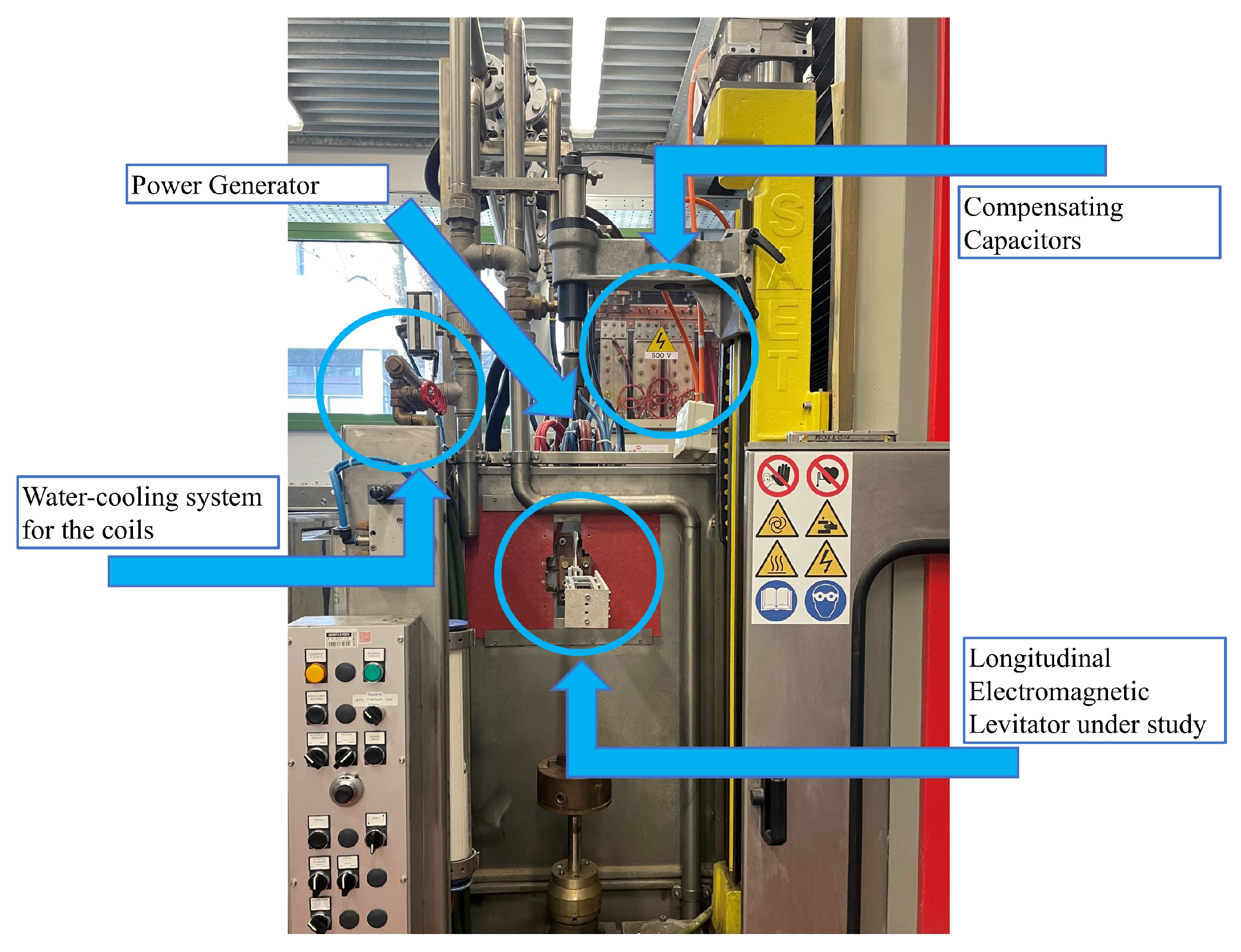
2. Device Under Study

The analysis presented in this paper is based on the LEL configuration shown in Figure 1. The device, with the conductor barycenter coordinates listed in

Table 1. Coordinates of the barycenter of the conductors presented in Figure 1b.

Barycenter	1	1′	2	2′	3	3′	4	4′
$x \left[\mathrm{mm}\right]$	$-15.5$	$15.5$	$-26$	26	$-26$	26	$-23.5$	$23.5$
$y \left[\mathrm{mm}\right]$	$-11.5$	$-11.5$	$4.5$	$4.5$	$20.5$	$20.5$	$36.5$	$36.5$

and overall dimensions shown in Figure 2, comprises two water-cooled coils made of copper tubing with a cross section of $9 \times 9 \times 2 \mathrm{mm}$, connected in parallel. Typically, inductors used in electromagnetic levitation systems consist of two main components, often realized as separate coils: the lifting coil, which generates the levitation force, and the stabilizing coil, which ensures the dynamic stability of the levitated object [23].

The device under study is designed to levitate an aluminum cylinder with a diameter of $25.4 \mathrm{mm}$, a length of $200 \mathrm{mm}$, and a mass of $267 \mathrm{g}$. The axes of the chosen reference system are shown in Figure 1b, with the z axis oriented orthogonally to the plane.

Unlike the device examined in [17], which operates at two different frequencies and currents for heating and levitation, the LEL proposed here uses a single frequency. This simplifies the power supply system and minimizes potential crosstalk between generators. However, the operational frequency must be carefully chosen to optimize both the lifting and heating performance. It is important to emphasize that this study focuses exclusively on maximizing the lifting capacity, with the heating function reserved for future research.

2.1. Electromagnetic Modeling

A common approach for modeling LELs is to employ a two-dimensional approximation of the device [5,10]. Such models allow for evaluating the current distribution inside the billet and the electromagnetic forces acting on it by considering the problem as a two-dimensional slice of an infinitely long device. While this approach is computationally efficient, the assumption does not hold when considering conductors of different lengths and otherwise ignored interactions at the start and end of the billet. A more accurate, albeit computationally intensive, approach is to create a three-dimensional model of the device to perform a more complete study, capturing the aspects that are not well described through the two-dimensional approximation.

The 3D eddy currents problem for a current-controlled coil in phasor notation can be described with the A-formulation [24]:

$$\nabla \times \nu \nabla \times \overline{\mathit{A}}+j\omega {\displaystyle \frac{1}{\varrho }}\overline{\mathit{A}}={\overline{\mathit{J}}}_s,$$

(1)

where $\overline{\mathit{A}}$ represents the magnetic vector potential phasor, $\varrho$ the electrical resistivity, ${\overline{\mathit{J}}}_s$ the source current density, $\omega =2\pi f$ the angular frequency, $\nu$ the magnetic reluctivity, and j as the imaginary unit. For the planar model, Equation (1) takes the form of [24]

$$\nabla ·\nu \nabla {\overline{A}}_z+j\omega {\displaystyle \frac{1}{\varrho }}{\overline{A}}_z=-{\overline{J}}_{sz},$$

(2)

where the z subscript indicates that $\overline{\mathit{A}}$ and ${\overline{\mathit{J}}}_s$ are nonzero only in the z direction, orthogonal to the plane. The two coils are connected in parallel and fed by an imposed current distributed on their cross sections. The time-averaged Lorentz force density acting in a generic position $\mathit{r}$ in the billet can be calculated in time-harmonic conditions by [2,22]

$$F\left(\mathit{r}\right)={\displaystyle \frac{1}{2}}\Re (\overline{J}\left(\mathit{r}\right)\times {\overline{B}}^{*}\left(\mathit{r}\right)),$$

(3)

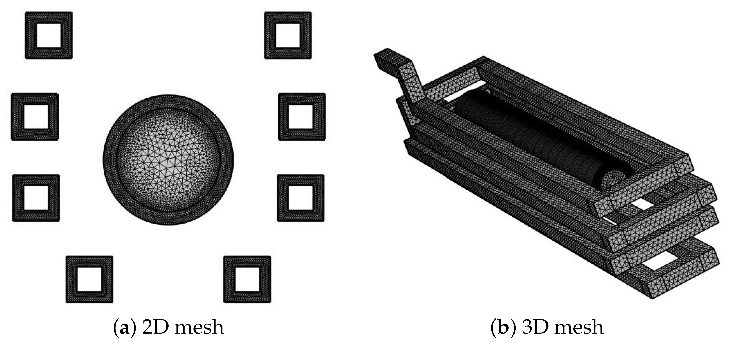
where ${\overline{B}}^{*}$ is the complex conjugate of the magnetic field phasor, and $\overline{J}$ is the induced current density in the load. It should be noted that the imaginary part of the cross product in Equation (3) represents a swing term at twice the source current frequency. Using the FEA software COMSOL Multiphysics^® 6.2, (1) and (2) were discretized using the meshes provided in Figure 3.

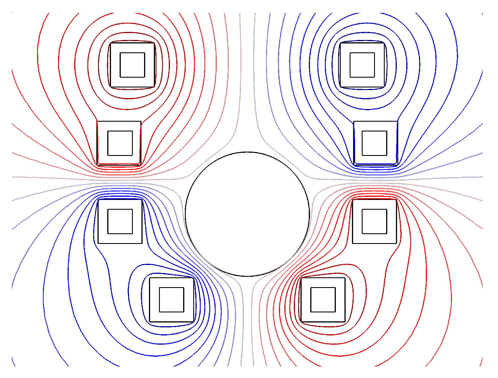
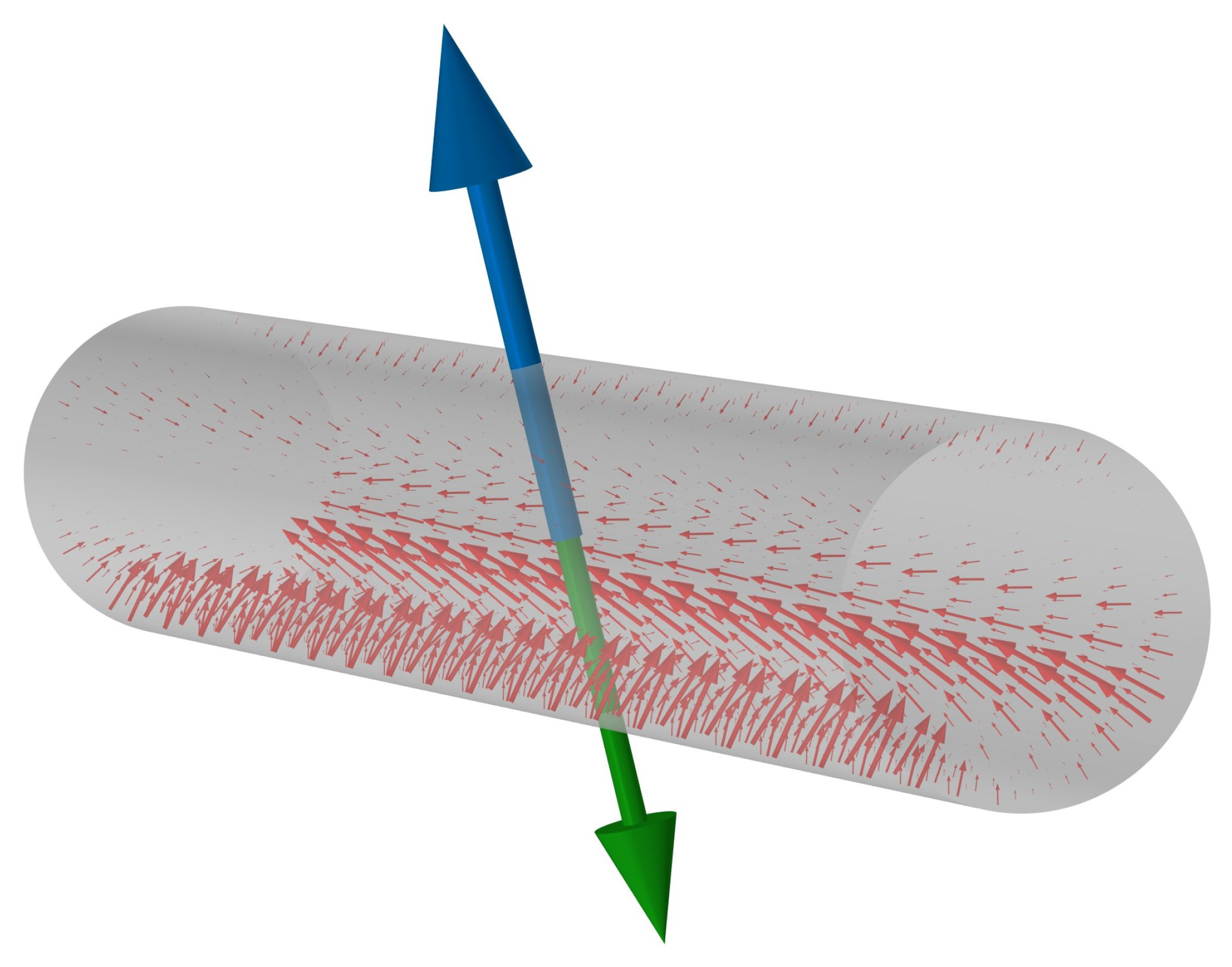
A 2D visualization of a typical solution for the device under study is presented in Figure 4, where the magnetic field contours are drawn for a specific current, frequency, and billet position, while a 3D visualization of Lorentz force within the billet at a certain position is shown in Figure 5. In the figure, red arrows indicate the local Lorentz force distribution, the blue arrow represents the resultant Lorentz force, and the green arrow denotes the gravitational force.

2.2. Coupled Electro-Thermal Simulation

Eddy currents induced in the workpiece, responsible for its levitation, produce Joule losses, increasing the temperature of the billet. Considering that the main purpose of the levitator under study is containment rather than melting, a thermal model is necessary to estimate the maximum containment time before the melting point is reached. The thermal transient inside the billet is described by the heat conduction equation for the temperature T [25]:

$$\rho c{\displaystyle \frac{\partial T}{\partial t}} = \nabla ·\left(k\nabla T\right)+q,$$

(4)

where $\rho$ is the density, c the heat capacity, and k the thermal conductivity. In Equation (4), q represents the Joule losses dependent on the electrical resistivity of the material $\varrho$:

$$q = \varrho \left(T\right){\left|\overline{J}\right|}^2.$$

(5)

Moreover, $c\left(T\right)$ and $k\left(T\right)$ represent the temperature-dependent heat capacity and thermal conductivity of aluminum, whose values are reported in

Table 2. Temperature dependence of electrical and thermal material properties of aluminum [26].

T (K)	$\mathit{\varrho }$ ($\mathbf{\Omega }\mathbf{m}·{10}^{-8}$)	c ($\frac{\mathbf{J}}{\mathbf{kgK}}$)	$\mathit{\lambda }$ ($\frac{\mathbf{W}}{\mathbf{mK}}$)
200	1.6	802	237
250	2.24	861	235
273	2.5	880	236
293	2.72	893	237
313	2.94	902	238
333	3.17	908	239
353	3.41	914	240
373	3.64	920	240
473	4.78	965	238
573	5.99	1030	233
673	7.3	1080	228
773	8.57	1130	222
873	9.77	1210	215
973	24.8	1080	92.1
1073	26.3	1080	95.5
1173	27.8	1080	98.6

[26].

The following convection and surface-to-ambient radiation conditions [25,27] are applied at the lateral surface of the billet:

$$-k{\displaystyle \frac{\partial T}{\partial n}}=h(T-T_{\mathrm{amb}})$$

(6)

$$-k{\displaystyle \frac{\partial T}{\partial n}}=\epsilon {\sigma }_B(T^4-T_{\mathrm{amb}}^4),$$

(7)

where $T_{amb}=293.15 \mathrm{K}$ is the ambient temperature, $h=10$ W/m² K represents the convection coefficient, ${\sigma }_B$ is the Stefan–Boltzmann constant, and $\epsilon =0.2$ is the emissivity of aluminum.

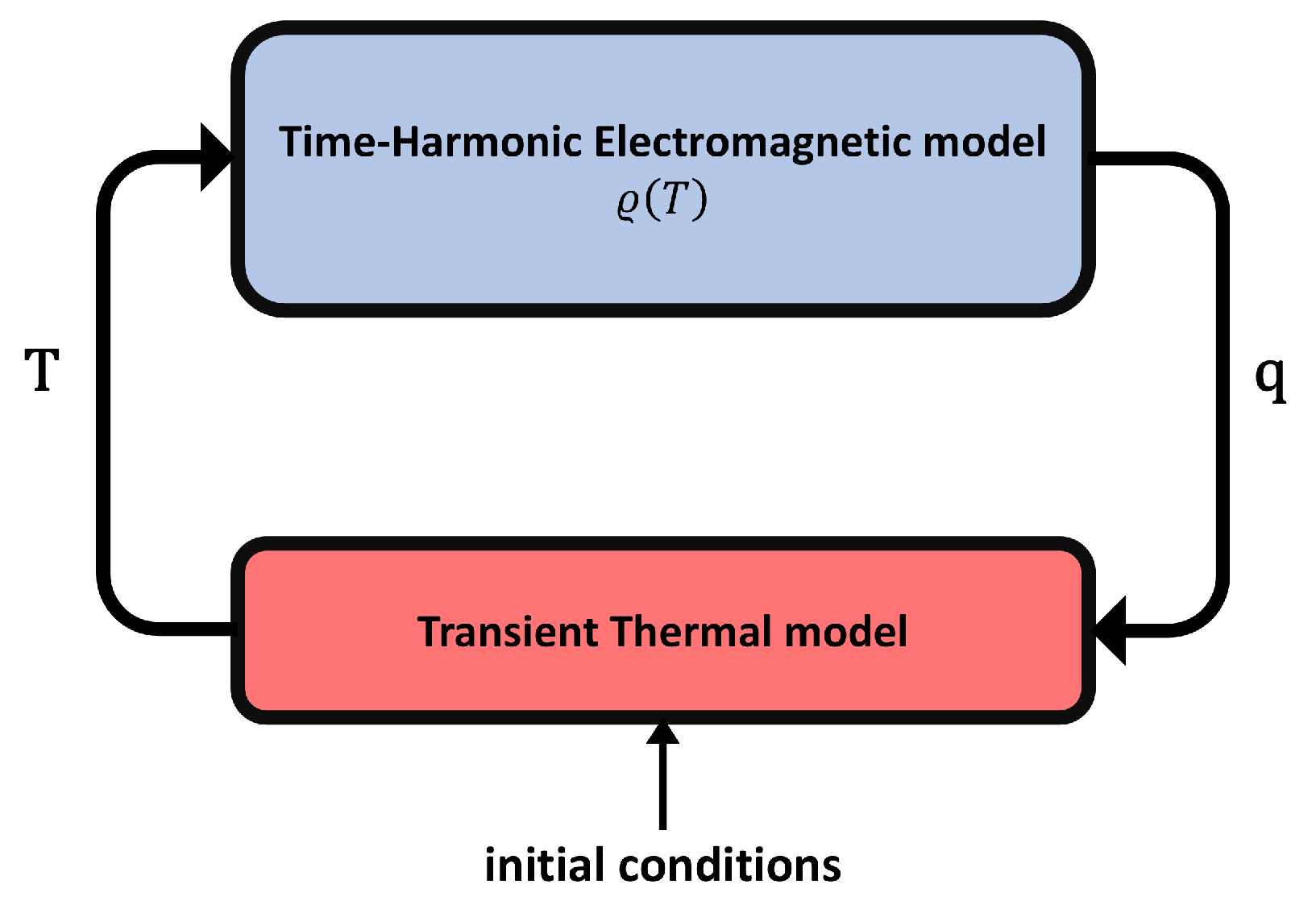
It should be noted that the temperature distribution of Equation (4) affects the electrical resistivity in Equation (2), which in turn changes the thermal power distribution in Equation (4). To estimate the transient temperature distribution, a coupled simulation between Equations (4) and (2), presented visually in Figure 6, must be performed.

3. Analysis of Stability

The stability analysis of the aluminum sample was conducted to determine the most suitable current and frequency values that ensure the sample’s levitation while minimizing the power deposition in the billet. For the sample to remain at a fixed position, the following condition must hold:

$${\displaystyle \frac{d^{2}y}{d{t}^2}}=0,$$

(8)

which indicates no acceleration. This condition can be verified by finding the point $y_{eq}$, where the lifting force balances the gravitational force. However, the absence of a net force at equilibrium does not inherently guarantee the stability of the billet at that point, particularly if equilibrium is reached through a mechanical transient. Since the load initially starts from a non-equilibrium position, it undergoes a transient motion, potentially reaching equilibrium with a non-zero velocity, leading to oscillations around the equilibrium position. This phenomenon has been observed in past research [28]. Equations (1) and (2) do not account for motional terms, meaning they cannot describe the transient displacement of the billet or the damping effects that may occur near equilibrium due to dissipative forces. Since the primary goal of this study is to identify the current and frequency values that allow the lifting force to counteract gravity precisely, for the remainder of this work, equilibrium is defined as the state where these forces are equal and opposite, without further consideration of damping effects. Moreover, given that the operating frequency is in the order of one $\mathrm{kHz}$, the oscillatory force component at twice this frequency can be considered negligible for equilibrium determination, as it primarily induces vibrations rather than significant displacement. Therefore, the following analysis will focus solely on the time-averaged component of the force.

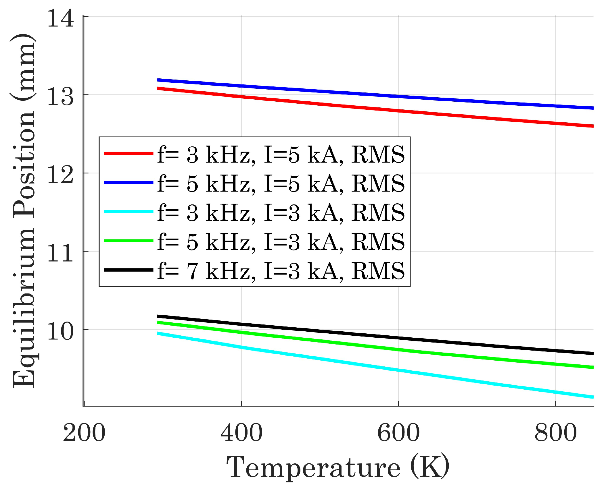
Furthermore, since the resistivity of aluminum increases with temperature, as shown in Table 2, the magnitude of the induced current varies throughout the device’s operation. The 3D FEM model has been employed to assess the impact of this variation of resistivity on the equilibrium position. Specifically, as shown in Figure 7, the equilibrium position of the billet decreases as the temperature rises. This trend is explained by the fact that the resistivity of the billet increases approximately linearly with the temperature.

The equilibrium position must be sufficiently distant from the lower excitation conductors [17] to prevent potential contact during the billet’s oscillatory motion. Therefore, in this study, the following equilibrium analysis is conducted under the assumption that the billet is at a temperature of $850 \mathrm{K}$. This value was selected as a reasonable upper limit for the process, as the goal is to achieve levitation of the billet without reaching its melting point.

The study was carried out by solving the electromagnetic problem for various vertical positions of the sample and different current and frequency values. For each case, the time-averaged lifting force was computed and compared to the gravitational force acting on the billet. Since this process requires solving the FEM model across multiple vertical positions, relying solely on the 3D model would be computationally expensive. Therefore, a comparison between the vertical equilibrium positions evaluated using the 3D and 2D models is necessary. 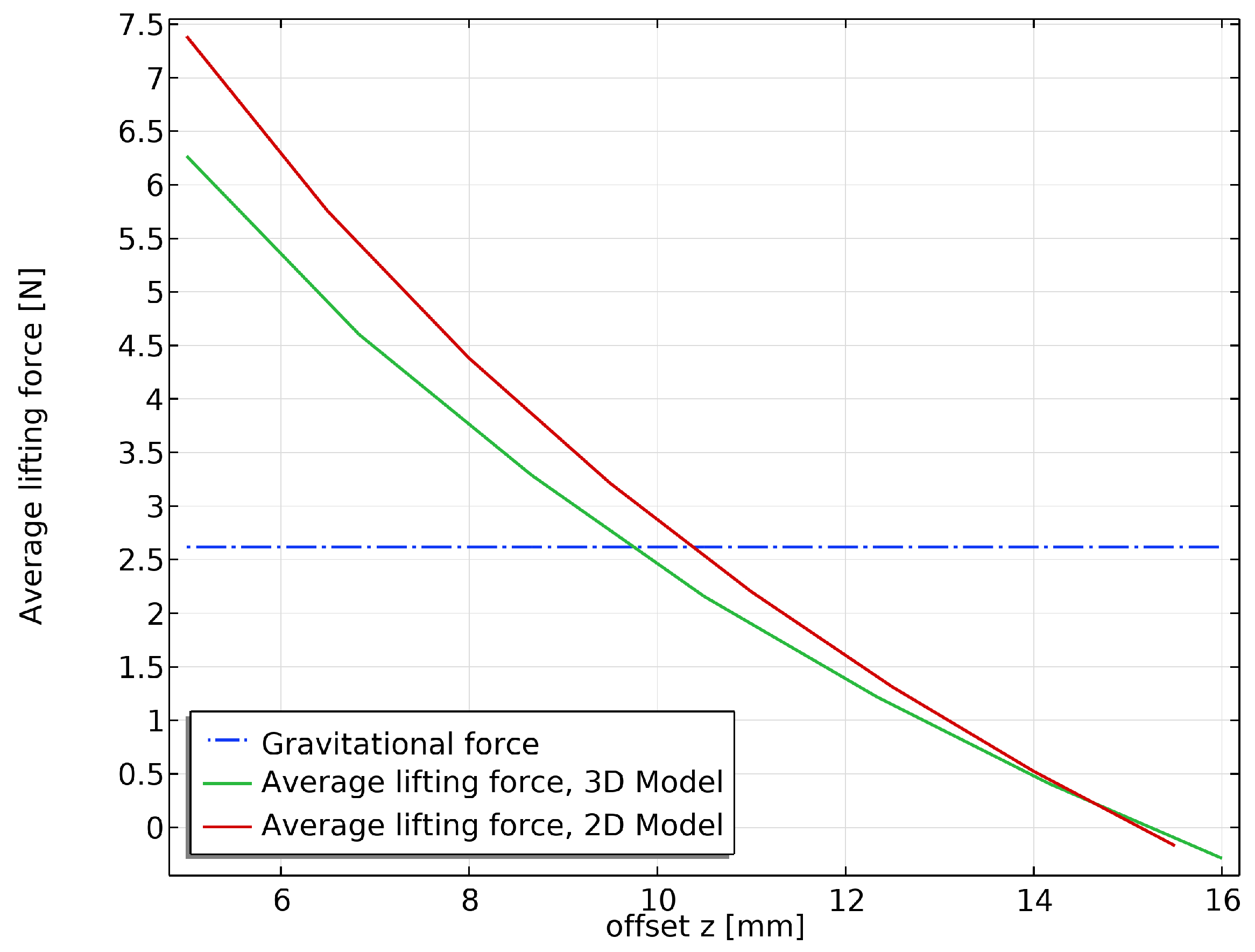Figure 8 illustrates the differences between the two models in evaluating the vertical average lifting force, considering a working frequency of $7 \mathrm{kHz}$ and a current of $3 \mathrm{kA},\mathrm{RMS}$. Specifically, the 2D model predicts the equilibrium position at a vertical height of $10.3 \mathrm{mm}$, whereas the 3D model predicts it at $9.7 \mathrm{mm}$. This indicates that the 2D model estimates the vertical position with an error of about 6% while significantly reducing the computational cost of the analysis.

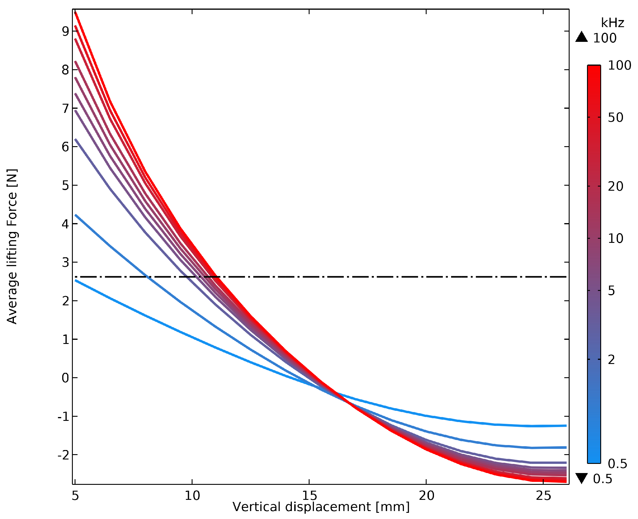
Once the reliability of the 2D model was assessed, the most suitable values of frequency and current were selected, relying on this model. To study the relationship between levitation conditions and current frequency, a study was performed for a set of frequencies from $50 \mathrm{Hz}$ to $100 \mathrm{kHz}$, imposing an arbitrary current value of $3 \mathrm{kA},\mathrm{RMS}$. Figure 9 illustrates the impact of the frequency on the average lifting force and, consequently, on the vertical equilibrium position of the sample seen in Figure 10. Figure 10 also displays the corresponding power induced in the load as the frequency increases, combining both effects in a single graph. The optimal frequency for the LEL under test is the one that ensures stable levitation at a vertical equilibrium position sufficiently distant from the lower exciting conductors while minimizing excessive heating of the load, as the device’s primary aim is not to melt the sample. Therefore, operating at frequencies higher than $5 \mathrm{kHz}$ is not suitable for the proposed application, as the power induced in the load increases without a corresponding significant rise in the vertical equilibrium position. Conversely, working at lower frequencies either prevents the establishment of a vertical equilibrium position or results in an equilibrium position too close to the lower conductors. Based on the frequency range of the available laboratory generator, the test was conducted at $7 \mathrm{kHz}$, which is the closest available frequency to the optimal one.

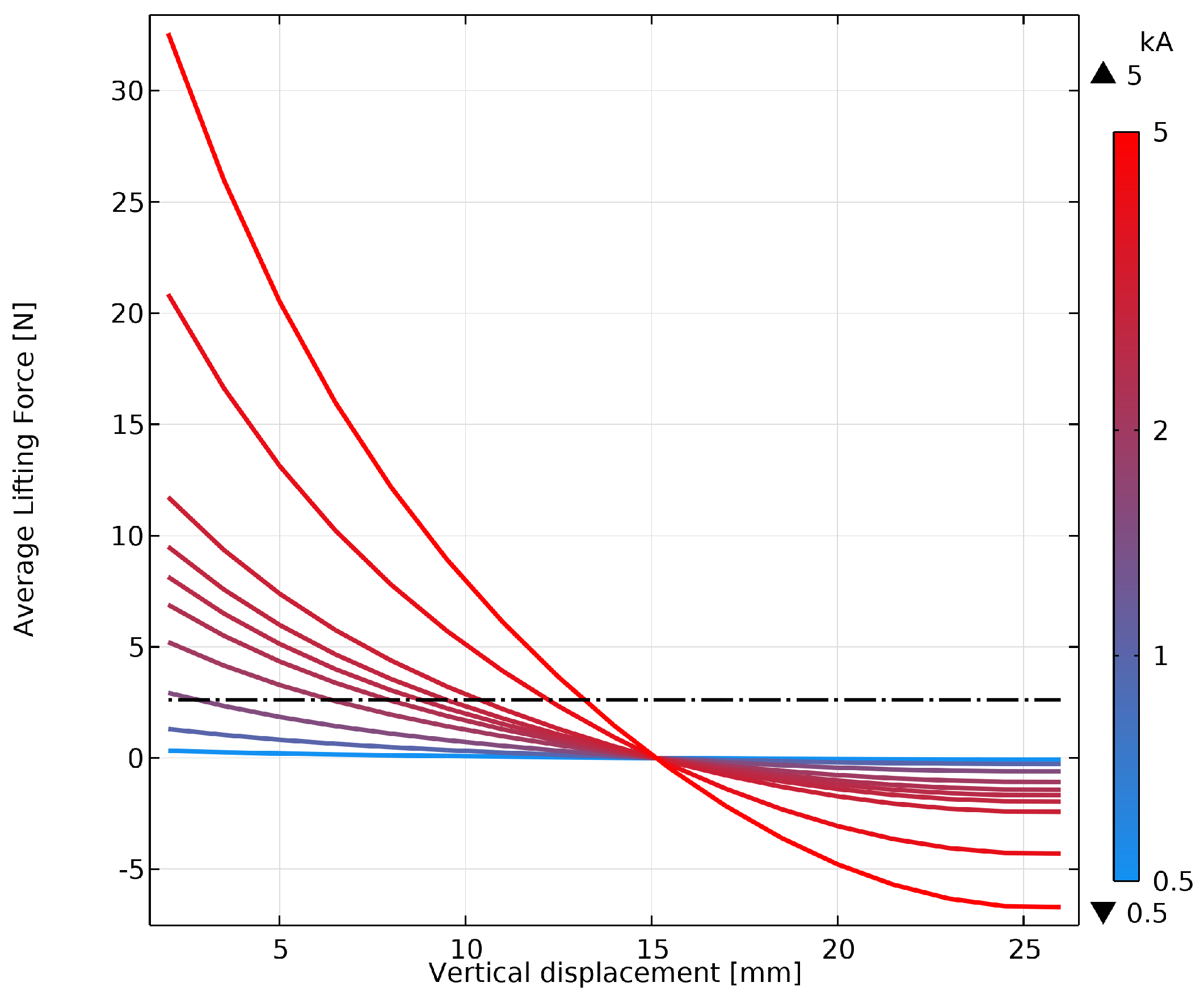
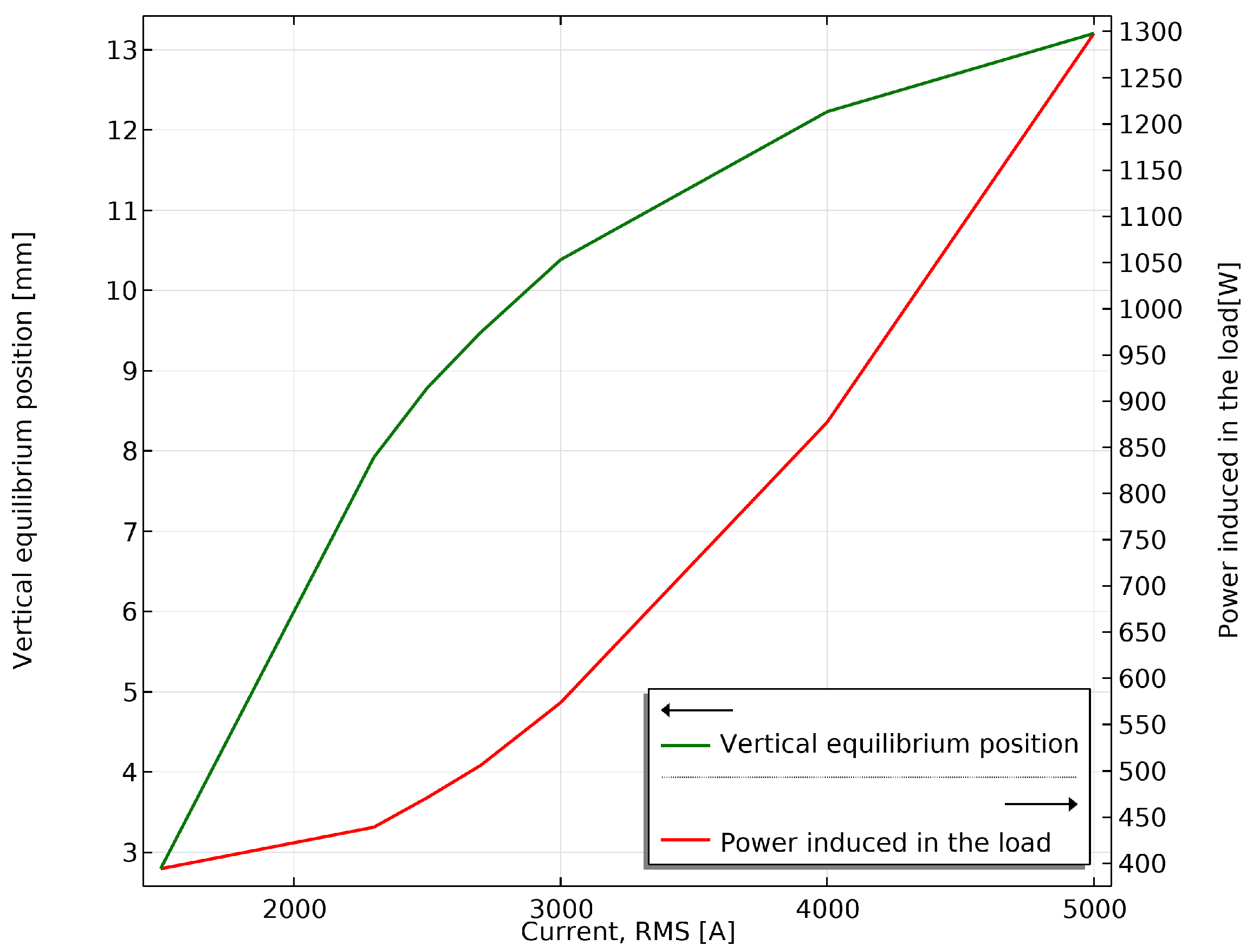
For what the choice of current concerns, a similar approach was adopted. In particular, as shown in Figure 11, a current sweep from $500 \mathrm{A},\mathrm{RMS}$ to $5 \mathrm{kA},\mathrm{RMS}$ was performed, imposing the overmentioned frequency of $7 \mathrm{kHz}$. As illustrated in Figure 12, the power induced in the load exhibits the typical quadratic dependence on the current. However, the vertical equilibrium position reduces the growth rate for currents exceeding $3 \mathrm{kA},\mathrm{RMS}$. Therefore, a good compromise in terms of current to achieve a noticeable lifting of the billet, while not inducing power on it, is to feed the inductor with a current of $3 \mathrm{kA},\mathrm{RMS}$.

Once the most suitable values of current and frequency were identified, a 3D simulation was performed to determine the precise equilibrium position, which was found to be $9.7 \mathrm{mm}$.

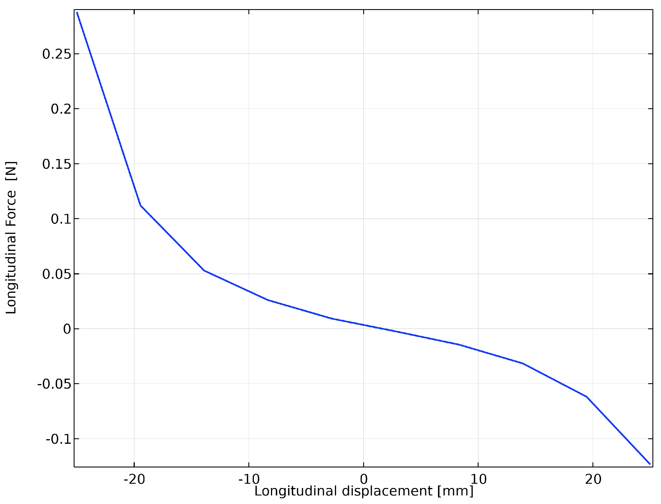
Two-dimensional analyses are essential for evaluating the vertical stability of the piece at the end of the mechanical transient. However, a comprehensive stability assessment must also consider longitudinal stability and the momentum stability of the sample. These aspects can only be examined through a 3D study, which accounts for the finite length of both the inductor and the piece, as well as the effects of longitudinal and lateral forces. 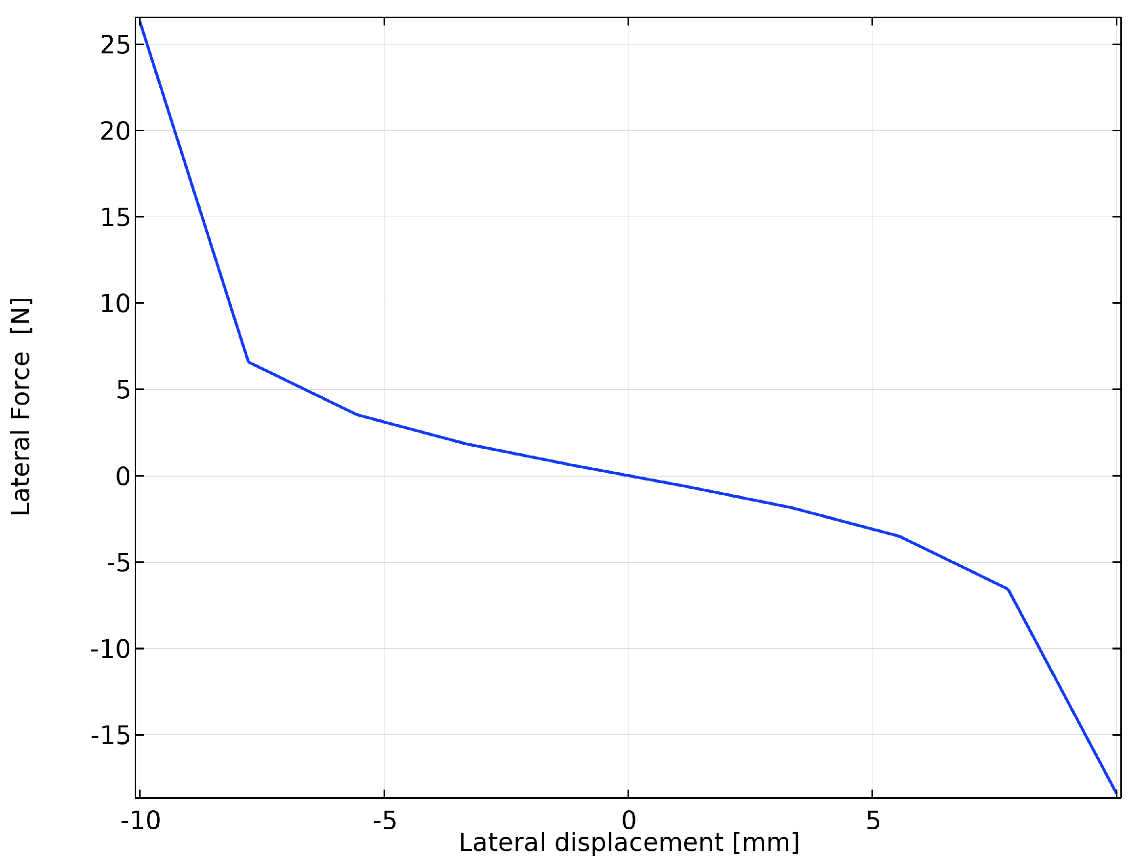As shown in Figure 13, the longitudinal force is positive when the center of mass of the piece is behind the inductor midpoint, and it is negative when it is ahead. This indicates that the longitudinal force consistently aligns the piece’s center of mass with the inductor longitudinal midpoint, thereby ensuring longitudinal stability. A similar effect is observed for the lateral force, as illustrated in Figure 14, which consistently acts to align the billet’s center of mass with the inductor’s lateral midpoint, thereby ensuring lateral stability. Comparable considerations apply to the piece’s rotation along the vertical and horizontal axes, corresponding to the y and x axes in the chosen reference system. Figure 15a,b illustrate the behavior of the torque with respect to the tilting angle of the piece. Notably, when the piece tilts away from its equilibrium position, the torque generates a restoring movement that drives the piece back to equilibrium. This self-correcting mechanism ensures rotational stability along both axes.

4. Coupled Electro-Thermal Simulation

As previously discussed in Section 2.1, the eddy currents responsible for levitating the billet also generate Joule losses, increasing the billet’s temperature. Since the primary purpose of the device is to levitate and confine the billet, without melting it, it is essential to determine the maximum allowable operating time (i.e., the time before the billet reaches its upper limit temperature) before experimenting. The upper limit temperature was identified at $850 \mathrm{K}$, to be sufficiently distant from the melting temperature. For this reason, a thermal model of the billet was derived.

It is important to remember that, according to Equations (4) and (5), the heating source of the thermal problem is represented by the Joule losses, which can be computed by solving the electromagnetic model. Furthermore, both the thermal and electrical material properties are dependent on the temperature, as reported in Table 2. The proper way to analyze this problem is, therefore, a fully coupled electro-thermal simulation.

Since performing this simulation on the 3D model would entail high computational costs, and the differences between the 2D and 3D models can be considered negligible, the electro-thermal analysis was conducted using the planar representation. The electric parameters adopted for the electromagnetic problem are the optimal ones selected in Section 3: a current of $3 \mathrm{kA},\mathrm{RMS}$, and a frequency of $7 \mathrm{kHz}$. Regarding the thermal problem, the boundary conditions described in Equations (6) and (7) were applied. Both convective heat flux and surface-to-ambient radiation were applied to the lateral surface of the billet.

In the simulation, the vertical position of the billet was set at $9.7 \mathrm{mm}$, which corresponds to the equilibrium position computed using the 3D model at a fixed temperature of $850 \mathrm{K}$. As previously discussed, this position depends on the electrical resistance of the billet, which in turn varies with the temperature. At the initial stage, when the billet’s temperature is still close to ambient, its actual equilibrium position is slightly higher. However, since the equilibrium position changes gradually with temperature (i.e., the slope of the curve in Figure 7 is relatively small), adopting the lower position as a constant throughout the simulation represents a reasonable approximation that does not significantly compromise the accuracy. Moreover, since the induced current in the billet is inversely proportional to the distance between the billet and the exciting conductors, fixing the position at the lower equilibrium position in the considered thermal operating range is a conservative assumption. This approach ensures that the simulation estimates the maximum induced power in the billet due to its position, resulting in a cautious approximation of the time-to-melt estimate.

The average temperature of the billet is then reported in Figure 16 until the melting temperature of $933 \mathrm{K}$ is reached. From this simulation, it is possible to see that the billet needs about 7 minutes to melt under the selected electrical parameters. Interestingly, the temperature increases approximately linearly over time despite the non-linear nature of the material properties. This behavior can be attributed to a balance: the enhanced heat loss from convection and radiation at higher temperatures is offset by the increased power deposition resulting from rising resistivity.

5. Experimental Setup and Test

The lifting capability of the studied LEL was verified in a laboratory scenario, feeding the inductor with a current of $3 \mathrm{kA},\mathrm{RMS}$ with a frequency of $7 \mathrm{kHz}$. The experimental setup used for the laboratory test is shown in Figure 17. The system consisted of a power generator with a nominal power of $275 \mathrm{kVA}$, equipped with a solid-state converter. The solid-state converter has a nominal power of $200 \mathrm{kW}$ and can deliver power within the frequency range of 5 to $30 \mathrm{kHz}$.

The initial position of the billet and the lifted position are reported in Figure 18a and Figure 18b, respectively.

From the experiment, it was observed that although the load was successfully lifted, the billet exhibited significant instability. This instability arises because the billet reaches the equilibrium position with a nonzero velocity, leading to sustained vertical oscillations around the equilibrium point. As discussed in [29], the superposition of a sufficiently high DC non-homogeneous magnetic induction can be used to stabilize both surface oscillations of melted materials and the motion of the center of gravity. Typical values are between 1 and 5 T for droplets [30]. These field intensities can be achieved through superconducting coils [31,32]. These aspects are of great interest to enhance the controllability of the sample and will be investigated in future research activities.

6. Conclusions

The lifting capacity of a longitudinal electromagnetic levitator (LEL) with single-frequency operation was examined. First, 2D and 3D numerical models were set up to establish the equilibrium position as a function of input parameters such as frequency and current. In particular, the 3D model was employed to improve the vertical equilibrium analysis initially conducted using the 2D model. It also accounts for the lateral and longitudinal displacements, as well as the torque effects around the billet’s principal axes. Moreover, the 3D model enables a more realistic representation by considering conductors of varying lengths and capturing electromagnetic interactions near the billet’s extremities.

The influence of temperature-dependent material properties was also considered, providing insights into the relationship between the billet’s equilibrium position and its temperature. Specifically, it was observed that the equilibrium position gradually decreases as the billet heats up during the levitation process.

For the proposed configuration, and in accordance with the technical limits of the laboratory’s power generator, an input current of 3 kA, RMS, at a frequency of 7 kHz was identified as optimal. These parameters ensured stable levitation of a $267 \mathrm{g}$ aluminum billet without causing it to melt within the intended operational time.

The simulation results were verified with experimental activities, highlighting the validity of the approach. Future research activities will be focused on optimizing the heating task and a further inspection of the oscillations seen in the numerical and experimental activities. In particular, it is highly desirable to reduce the oscillations by employing accurate control techniques.