Optimization and Estimation of the State of Charge of Lithium-Ion Batteries for Electric Vehicles

Abstract

Lithium batteries have become one of the best choices for current consumer electric vehicle batteries due to their good stability and high energy density. To ensure the safety and reliability of electric vehicles (EVs), the battery management system (BMS) must provide accurate and real-time information on the usage status of the onboard battery. This article highlights the precise estimation of the state of charge (SOC) applied to four models of lithium-ion batteries (Turnigy, LG, SAMSUNG, and PANASONIC) for electric vehicles in order to ensure optimal use of the battery and extend its lifespan, which is frequently influenced by certain parameters such as temperature, current, number of charge and discharge cycles, and so on. Because of the work’s novelty, the methodological approach combines the extended Kalman filter algorithm (EKF) with the noise matrix, which is updated in this case through an iterative process. This leads to the migration to a new adaptive extended Kalman filter algorithm (AEKF) in the MATLAB Simulink 2022.b environment, which is novel or original in the sense that it has a first-order association. The four models of batteries from various manufacturers were directly subjected to the Venin estimator, which allowed for direct comparison of the models under a variety of temperature scenarios while keeping an eye on performance metrics. The results obtained were mapped charging status (SOC) versus open circuit voltage (OCV), and the high-performance primitives collection (HPPC) tests were carried out at 40 °C, 25 °C, 10 °C, 0 °C and −10 °C. At these temperatures, their corresponding values for the root mean square error (RMSE) of (SOC) for the Turnigy graphene battery model were found to be: 1.944, 9.6237, 1.253, 1.6963, 16.9715, and for (OCV): 1.3154, 4.895, 4.149, 4.1808, and 17.2167, respectively. The tests cover the SOC range, from 100% to 5% with four different charge and discharge currents at rates of 1, 2, 5 and 10 A. After characterization, the battery was subjected to urban dynamometer driving program (UDDS), Energy Saving Test (HWFET) driving cycles, LA92 (Dynamometric Test), US06 (aggressive driving), as well as combinations of these cycles. Driving cycles were sampled every 0.1 s, and other tests were sampled at a slower or variable frequency, thus verifying the reliability and robustness of the estimator to 97%.

1. Introduction

The growing need for energy in multiple industrial sectors, including the automobile sector and electric vehicles, favors the rapid emergence of renewable energies [1]. The production of electrical energy from photovoltaic systems or even wind turbines represents a considerable alternative in the family of renewable energies [2]. Variations from climate data considerably influence the flow of energy production in multiple applications of integrating renewable energies into electric vehicles or in special industries [3]. The development of energy storage systems or devices, such as batteries, is essential and crucial for optimizing non-dependence on electrical energy [4]. Lithium batteries are therefore widely used and are currently the subject of several research issues by multiple industrial manufacturers for various applications such as electric vehicles. Several parameters are therefore positioned as performance indicators guaranteeing optimal functioning of lithium batteries. Among their indicators, the state of charge (SOC) is crucial, as it assesses the battery’s proper functioning and directly influences both its lifespan and the overall performance of the electric vehicle in this context [5]. Optimal estimation of the state of charge of batteries for electric vehicles will provide better performance for the electric vehicle, with an impact on the lifespan of the batteries [6]. Improving the accuracy of estimating the state of charge of batteries is therefore a scientific and technological issue of great importance.

1.1. Literature Review on State of Charge (SOC) Estimation Methods

Recent work in the literature reveals the existence of four large families of state of charge (SOC) estimation methods: the method integrating the Coulomb approach [7,8], the (OCV) method which evaluates the open circuit voltage [9,10], the associated dataset method [11] and the method based on approaches or even algorithmic models [12,13]. All these methods possess both advantages and limitations, including in their implementation. As for illustration, with the Coulomb approach, it is necessary or even imperative to have data on the initial state of the charging system. Moreover, it is deployed in an open loop, thus causing a considerable margin of error over time [14]. Still, another limitation for the (OCV) method, the length of time required for diffusion, constitutes a major drawback in the steady-state terminal voltage measurement process [15]. Intelligent and dataset-based methods also have implementation drawbacks [16,17]. The optimization process turns out to be very complex due to prior validation, which depends on several optimization criteria of the objective function of the system [18,19]. Several nonlinear control strategies, such as sliding mode, predictive control, and H∞ observer [20,21], have been tried to improve the uncertainties of the Intelligent Methods system. However, the difficult design of the state observer module does not facilitate optimal exploitation of nonlinear control strategies in these cases [22,23]. Thus, the methods associated with filters are positioned as the most used methods [24,25]. These methods generally integrate: battery models, algorithms allowing the identification of parameters, as well as filtering [26,27]. Electrochemical battery models and equivalent circuit models are the most cited in recent works [28,29]. However, equivalent circuit models offer the possibility of making an estimation of the state online, thanks to a good relationship between the precision and the complexity of the optimization coefficients of the objective function [30,31]. The Kalman filter approach offers multiple advantages for its cases or scenarios during the estimation process: (1) it is an online algorithm with closed-loop feedback with small numbers of variables not requiring exponential computing power (2) ease of implementation also integrating high precision in comparison with other methods in the literature such as the ampere-hour method [32,33] (3) it directly uses the state equation model to estimate the dynamic parameters whose inputs are generally: the current, the cell temperature and the output with the terminal voltage [34,35]. Using the traditional Kalman approach, limitations become evident in the State of Charge (SOC) index, particularly in issues such as shift, derivative inaccuracies, and long-term state divergence [36,37]. The reason why extended Kalman filter (EKF) algorithms have been proposed to resolve their limits [38,39]. In this case or scenario (EKF), the first order partial derivative of the Taylor expansion of the nonlinear function, a global simplification of higher order terms is carried out to facilitate linearization and good estimation by filtering [40]. The work [41] demonstrates the presence of persistent noise in the estimation process. They also develop an approach integrating fractional derivative theory with voltage-capacitance theory. This approach allows for the extraction of the CP from the fractional differential voltage and capacitance model, thus demonstrating the feasibility of extracting these parameters. It effectively circumvents the limitations associated with extracting features from integer-order derivative curves. However, the problem lies in the initial conditions. Several works in the literature present the advantages and limitations of estimation by the Kalman algorithm.

Table 1. Analysis of estimates with the Kalman algorithm.

Ref.	Themes	Dynamic Parameters	Benefits	Disadvantages
[42]	Optimization of the state of charge of lithium batteries with integration of the Kalman algorithm	State of charge, temperature, and current	15% reduction in error during load state estimation	Sensitivity to temperature variations, which can affect the accuracy of the estimate
[43]	Mitigation of the influence of temperature on the state of charge of lithium batteries with the Kalman algorithm	Battery age, charge cycles, temperature	Reduced the impact of temperature on state of charge estimation by 25%	Need adjustments for extreme temperature ranges
[44]	Comparison of Kalman algorithms in the management of lithium batteries for electric vehicles	Voltage, current, temperature	Comparison of methods and superiority of the Kalman algorithm	Accumulated modeling complexity for nonlinear systems
[45]	Improvement of charging and discharging of lithium batteries with the Kalman algorithm	Charging and discharging strategies	Extended battery life by 25%	Need for in-depth studies on the long-term impact of charging and discharging strategies
[46]	Optimizing Battery Life Using the Kalman Filter Algorithm in Electric Vehicles	Battery internal resistance, state of charge, discharge power	Extended battery life by 20%	Need for additional experimental validations for various driving profiles
[47]	Superiority of Kalman Filter Algorithm in State of Charge Estimation Compared to Machine Learning Methods	Machine Learning based methods, comparison with the Kalman algorithm	Superiority of Kalman algorithm with 85% accuracy	Need for additional comparisons with nonlinear methods for comprehensive evaluation
[48]	Evaluation of residual capacity of lithium batteries under variable load using Kalman filter algorithm	Residual capacity, load variations	Accurate estimation of residual battery capacity	Need for additional data for varied load scenarios
[49]	Experimental study of the effectiveness of the Kalman filter algorithm for the management of lithium batteries in electric vehicles	Experimental validation, agreement with real data	Experimental confirmation of the effectiveness of the Kalman filter algorithm	Sensitivity to experimental conditions that may affect validation
[50]	Predicting battery aging using multivariable models with the Kalman Filter algorithm	Battery aging, temperature, and charging cycles	Accurate prediction of battery aging	Sensitivity to variations in load conditions for long-term predictions
[23]	Adaptive energy management with Kalman filter algorithm for electric vehicle batteries	Variable driving profiles, adaptation to conditions	Development of adaptive models for efficient energy management	Limited adaptability to sudden changes in driving conditions
[17]	Estimation of long-term state of charge in lithium batteries using Kalman filter algorithm	Estimated load, long-term data	92% reliability in estimating the state of charge	Need for long-term studies to confirm reliability under various conditions

below presents this evolution. Dynamic variables or evolving parameters are also defined in order to better exploit the contributions presented in this work.

The paper [51] presents the data acquisition error in a battery management system, combined with the online parameter identification method based on recursive least squares (RLS). The state of charge (SOC) estimation method based on the extended Kalman filter (EKF) and the adaptive extended Kalman filter (AEKF) is established and tested in the federal urban driving program. Then, in the presence of noise interference on the input signal, the anti-interference of the three methods is compared. Finally, it is concluded that the AEKF method with innovation-based adaptive estimator provides the best noise suppression, with a state of charge estimation error of less than 2%. It constitutes the research basis for the application of EKF/AEKF methods to the current battery management system. Similarly, the paper [52] already demonstrates the advantages of the AEKF model over traditional methods. An improved version of this method has also been developed, and the results of its synthesis are presented. It then becomes necessary to have an adaptive evolution law, which is a function dependent on or associated with the dimension of the state vectors, as described by the parametric model developed in the remainder of this work.

1.2. Paper Contributions

Indeed, although the EKF and AEKF methods are traditional methods, their implementation depends on the choice and use of parameter estimation algorithms, which will enhance the robustness and accuracy of the system’s parameters during the overall implementation process [3]. Therefore, at this level, multiple avenues of research and optimization are developing, with the main mission of finding the best possible estimation method according to the system’s constraints. Several scientific researchers have developed applications of the EKF and AEKF algorithms with estimators based on: (i) Linear regression method, (ii) Least squares method (LSM), (iii) Bayes estimator method and each of these methods has advantages and disadvantages in the overall process of implementing the algorithm. This is why in the present work, the precise knowledge of the system model and the dynamics of its parameters is based on an iterative method integrating the second-order Taylor development, which combines the proposal of an estimator applied to a first-order Thevenin model to strengthen the robustness and precision of the system parameters. This methodological mixture makes it possible to resolve the limits developed by [1,42]. In addition, this work develops a comparative study of four lithium battery manufacturers (Turnigy, LG, SAMSUNG, PANASONIC) for temperatures of 40 °C, 25 °C, 10 °C, 0 °C and −10 °C, and whose internal parameters of these different models are identified by linear second-order Taylor development with the adapted Extended Kalman Filter algorithm.

The different operating scenarios for temperatures ranging from 40 °C to −10 °C allow us to test the performance of our algorithm by also performing the update of the process noise covariance and the measurement noise covariance adaptively to improve the state of charge estimation process, with a simplification of the computing power while maintaining high accuracy and good stability. Its results are in accordance with ISO 12405-4, IEC 61982 standards and with one of the results of [1,2]. These results therefore provide a good understanding of the performance of electric vehicles in hot tropical areas and cold areas during winter, and will allow manufacturers to significantly improve production models by making them more efficient. In addition, the work [53] highlights a risk assessment framework based on the conditional value at risk (CVaR). This will allow for a better description of the evolution of the noise matrix. Therefore, the main contributions in this work are the following:

(a)

Optimal noise suppression and better temporal control of the covariance matrix in the battery SOC estimation process.

(b)

An assessment of the accuracy and robustness of the SOC estimation by determining a range within which online noise covariance updates are possible for good noise estimation over time.

(c)

The proposed simulation conditions are very close to industrial reality, as parameter estimation varies greatly depending on the technologies used by battery manufacturers. Data are estimated in a highly variable manner depending on the online experimental conditions of different manufacturers, although the technical operating characteristics of the batteries vary considerably within the same ranges. This reality makes the simulation protocol highly stochastic, which represents a major challenge for this study. Emphasis is placed on highlighting the chaotic fluctuations recorded during model estimation and validation using stability margins.

(d)

A case study of four lithium battery manufacturers (Turnigy, LG, SAMSUNG, PANASONIC) for temperatures of 40 °C, 25 °C, 10 °C, 0 °C and −10 °C, and whose internal parameters of these different models are identified by second-order linear Taylor development with a positioning in relation to the literature and current standards with recommendations for sustainable development of the automotive sector.

1.3. Organization of the Article

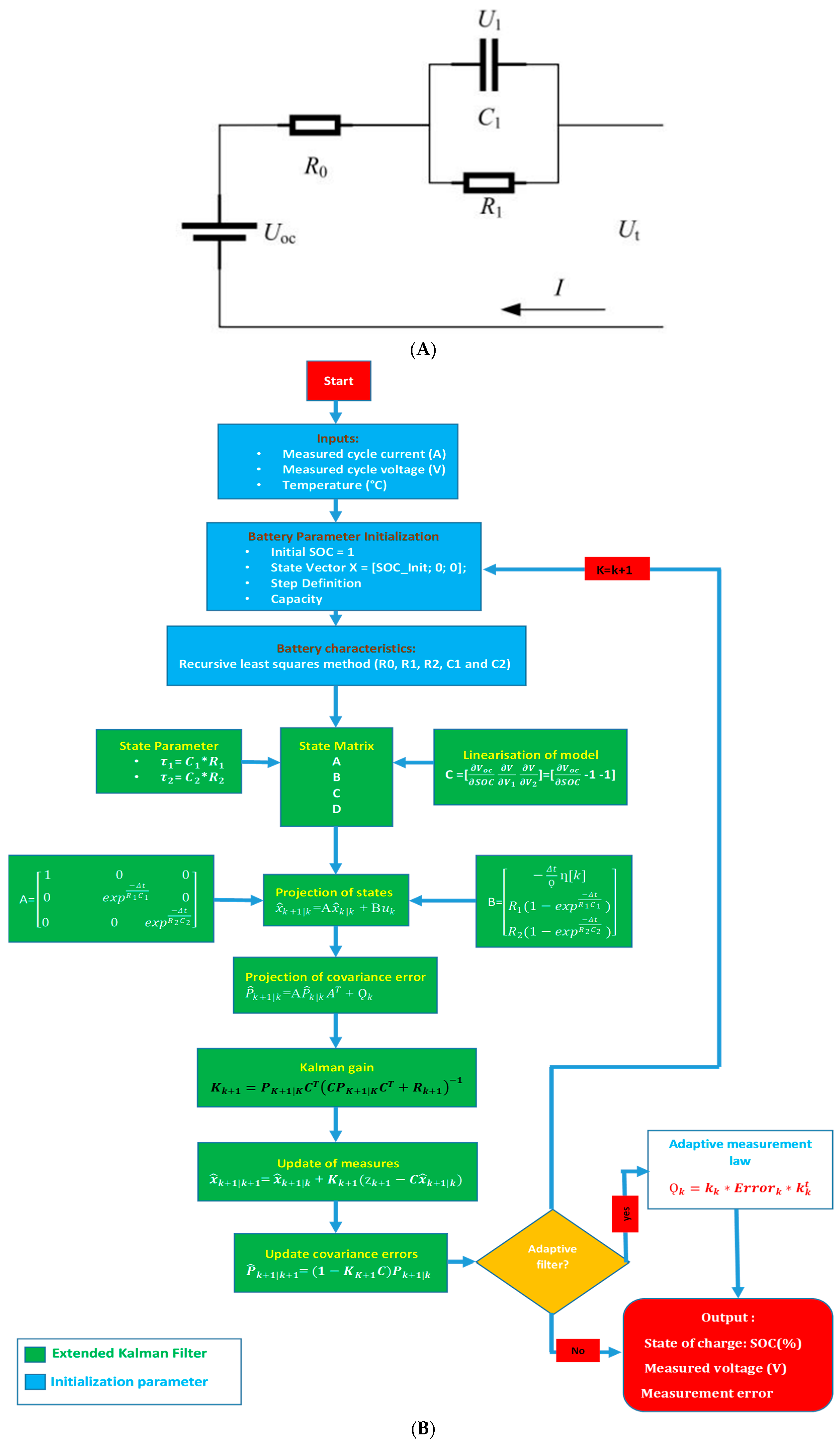
In the remainder of this paper, Section 2 presents a complete system model, including the battery architecture and parameter estimation by the least squares method. This approach allows accurate simulations of four lithium battery models at different operating temperatures in the MATLAB Simulink 2018b environment. Section 3 presents the results obtained and the necessary discussions from the four lithium battery models, as well as an analysis of the influence of temperature and experimental simulation conditions on different operating scenarios. Finally, Section 4 concludes by recalling the challenges and interesting contributions of this article in the automotive sector, and in particular, the multiple possibilities offered by photovoltaic energy production applications, with future research perspectives.

2. System Modeling

2.1. Battery Architecture

In this work, the first-order Thevenin equivalent circuit model is used to describe the battery characteristics. The equivalent circuit diagram is shown in Figure 1A below.

$$\left\{\begin{array}{c}{U}_1={\displaystyle \frac{\dot{I}}{C_1}}-{\displaystyle \frac{U_1}{R_1{C}_1}}\\ U_t=U_{oc}-{IR}_0-U_1\end{array}\right.$$

(1)

where U_oc is the open circuit voltage, U_t represents the terminal voltage, R₁ and R₀ represent the resistance, and C₁ represents the capacitance. The SOC of a cell is expressed by:

$$SOC\left(t\right)=SOC\left(t_0\right)-{\int }_{t_0}^{t_0+∆t}{\displaystyle \frac{\eta I\left(t\right)dt}{Q_n}}$$

(2)

SOC(t) and SOC(t₀) represent the current and initial SOC values, respectively. Q_n represents the maximum available capacity, and η represents the Coulomb efficiency. When using the Adapted Extended Kalman Filter (AEKF) to accurately estimate the state of charge (SOC), accurate model parameters are essential. Since the recursive least squares method (RLM) has high recognition accuracy and fast convergence speed, in this work, we will use this method to identify the parameters of the online model. Applied to the Laplace transform to the second equation of Equation (1), gives:

$$U_{oc}(s)-U_t(s)=I\left(s\right)\left(R_0+{\displaystyle \frac{R_1}{1+R_1{C}_{1}s}}\right)$$

(3)

We can then obtain the transfer function Equation (4).

$$G\left(s\right)={\displaystyle \frac{U_{oc}\left(s\right)-U_t\left(s\right)}{I\left(s\right)}}=\left(R_0+{\displaystyle \frac{R_1}{1+R_1{C}_{1}s}}\right)$$

(4)

In the discrete domain, by replacing s by: s = 2(1 − z⁻¹)/T(1 + z⁻¹). Then, Equation (5) is obtained by bilinear transformation:

$$G\left(z\right)={\displaystyle \frac{a_2+a_3{z}^{-1}}{1+a_1{z}^{-1}}}$$

(5)

The difference Equation (6) can be obtained according to the discretized transfer function (5)

$$y\left(k\right)=U_{oc}\left(k\right)-U_t\left(k\right)=-a_{1}y\left(k-1\right)+a_{2}I\left(k\right)+a_{3}I(k-1)$$

(6)

where y(k) represents the output of the model and I(k) is the input. Defined by:

$$\left\{\begin{array}{c}{\Phi }_k=[-y\left(k-1\right), I\left(k\right),I\left(k-1\right)]\\ {\theta }_k=\left[\begin{array}{c}{a}_1\\ a_2\\ a_3\end{array}\right]\end{array}\right.$$

(7)

$$y\left(k\right)={\Phi }_k{\theta }_k$$

(8)

with:

$$\left\{\begin{array}{c}{a}_1={\displaystyle \frac{1-2\tau }{1+2\tau }}\\ a_2={\displaystyle \frac{R_0+R_1+{2R}_0\tau }{1+2\tau }}\\ a_3={\displaystyle \frac{R_0+R_1-{2R}_0\tau }{1+2\tau }}\end{array}\right.$$

(9)

where τ = R₁C₁. According to Equations (8) and (9), a₁, a₂, and a₃ can be solved using Recursive Least Squares (RLM), and each parameter of the battery model can be obtained

2.2. Parameter Estimation

In the present work, the nonlinear function is approximated to a linear function by a second-order Taylor expansion, and the third-order and higher terms are ignored in order to reduce the truncation error. If the approximate order is further increased, the accuracy is not significantly improved, and the computational cost of the algorithm will increase. Therefore, considering the estimation accuracy and the calculation amount, the equilibrium for the adapted Extended Kalman Filter (AEKF), the second-order Taylor approximation is a common choice in the literature.

The nonlinear system is expressed by the following equation:

$$\left\{\begin{array}{c}{x}_{k+1}=f\left(x_k,u_k\right)+{\omega }_k\\ y_{k+1}=g\left(x_k,u_k\right)+{\nu }_k\end{array}\right.$$

(10)

where w_k represents process noise, v_k represents the measurement noise, x_k+1 and y_k+1 represent the state vector and the observation vector, respectively. f represents the state equation of the system, and g represents the measurement equation of the system, both of which are nonlinear functions. Their discretization makes it possible to establish the state Equation (11) and the measurement Equation (12) switch to battery mode.

$$\left\{\begin{array}{c}{U}_{1,k+1}=U_{1,k}{e}^{-1/\left(R_1{C}_1\right)}+I_k{R}_1(1-e^{-1/\left(R_1{C}_1\right)})\\ {SOC}_{k+1}={SOC}_k-{\displaystyle \frac{I_k}{Q_n}}\end{array}\right.$$

(11)

$$U_{t,k}=U_{oc,k}-U_{1,k}-I_k{R}_0$$

(12)

where x_k+1 = [U_1,k+1,SOC_k+1]^T, y_k+1 = U_t,k+1, and U_oc,k is a SOC polynomial. The seventh-order polynomial is used to describe the functional relationship between SOC and U_oc,k. The second-order Taylor expansion of the state equation is discussed in the form of Equation (13):

$$f\left(x\right)\approx f\left({\widehat{x}}_{k-1}\right)+{\left.{\displaystyle \frac{\partial f}{\partial x}}\right|}_{{\widehat{x}}_{k-1}}\left(x_{k-1}-{\widehat{x}}_{k-1}\right)+{\displaystyle \frac{1}{2}}{\sum }_{i=1}^{n_x}{l}_i{\left(x_{k-1}-{\widehat{x}}_{k-1}\right)}^T{\left.{\displaystyle \frac{{\partial }^2{f}_i}{\partial x^2}}\right|}_{{\widehat{x}}_{k-1}}\left(x_{k-1}-{\widehat{x}}_{k-1}\right)$$

(13)

where n_x represents the dimension of the state vector and l_i is the basis vector in the ith dimension n_x. The state vector can be converted to:

$$x_k\approx f\left({\widehat{x}}_{k-1}\right)+{\left.{\displaystyle \frac{\partial f}{\partial x}}\right|}_{{\widehat{x}}_{k-1}}\left(x_{k-1}-{\widehat{x}}_{k-1}\right)+{\displaystyle \frac{1}{2}}{\sum }_{i=1}^{n_x}{l}_i{\left(x_{k-1}-{\widehat{x}}_{k-1}\right)}^T{\left.{\displaystyle \frac{{\partial }^2{f}_i}{\partial x^2}}\right|}_{{\widehat{x}}_{k-1}}\left(x_{k-1}-{\widehat{x}}_{k-1}\right)$$

(14)

We can get Equation (15) from Equation (14).

$$x_k\approx f\left({\widehat{x}}_{k-1}\right)+{\left.{\displaystyle \frac{\partial f}{\partial x}}\right|}_{{\widehat{x}}_{k-1}}\left(x_{k-1}-{\widehat{x}}_{k-1}\right)+{\displaystyle \frac{1}{2}}{\sum }_{i=1}^{n_x}{e}_{i}tr{\left.({\displaystyle \frac{{\partial }^{2f_i}}{\partial x^2}}\right|}_{{\widehat{x}}_{k-1}}{P}_{k-1})+{\omega }_{k-1}$$

(15)

The second-order Taylor series of g(x) can be written as:

$$g\left(x\right)\approx g\left({\widehat{x}}_{k-1}\right)+{\left.{\displaystyle \frac{\partial g}{\partial x}}\right|}_{{\widehat{x}}_{k-1}}\left(x_{k-1}-{\widehat{x}}_{k-1}\right)+{\displaystyle \frac{1}{2}}{\sum }_{i=1}^{n_x}{l}_i{\left(x_{k-1}-{\widehat{x}}_{k-1}\right)}^T{\left.{\displaystyle \frac{{\partial }^2{g}_i}{\partial x^2}}\right|}_{{\widehat{x}}_{k-1}}\left(x_{k-1}-{\widehat{x}}_{k-1}\right)$$

(16)

To obtain the algorithmic steps of the second-order AEKF, it is essential to first obtain the iterative steps of the second-order FEK (SOFEK). The basic steps of the Extended Kalman Filter (FEK) algorithm are represented by the following Equations (17)–(20)

(a)

Initialization

$$\left\{\begin{array}{c}{\widehat{x}}_0=E\left(x_0\right)\\ P_0=E\left[\left(x_0-{\widehat{x}}_0\right){\left(x_0-{\widehat{x}}_0\right)}^T\right]\end{array}\right.$$

(17)

(b)

Time update

$$\left\{\begin{array}{c}{\overline{x}}_k=f\left({\widehat{x}}_{k-1}\right)+{\displaystyle \frac{1}{2}}{\sum }_{i=1}^{n_x}{e}_{i}tr{\left.({\displaystyle \frac{{\partial }^{2f_i}}{\partial x^2}}\right|}_{{\widehat{x}}_{k-1}}{P}_{k-1})\\ {\overline{P}}_k={\Phi }_{\left.k\right|k-1}{P}_{k-1}{{\Phi }_{\left.k\right|k-1}}^T+{\displaystyle \frac{1}{2}}{\sum }_{i=1}^{n_x}{\sum }_{j=1}^{n_x}{e}_i{e}_j^{T}tr [{\left.{\displaystyle \frac{{\partial }^2{f}_i}{\partial x^2}}\right|}_{{\widehat{x}}_{k-1}}{P}_{k-1}{\left.{\displaystyle \frac{{\partial }^2{f}_i}{\partial x^2}}\right|}_{{\widehat{x}}_{k-1}}{P}_{k-1}]+Q_{k-1}\end{array}\right.$$

(18)

(c)

Kalman gain

$$\left\{\begin{array}{c}{K}_k=P_{\left.k\right|k-1}{C}_k^T{S}_k^{-1}\\ S_k=C_k{P}_{\left.k\right|k-1}{C}_k^T+{\displaystyle \frac{1}{2}}{\sum }_{i=1}^{n_x}{\sum }_{j=1}^{n_x}{e}_i{e}_j^{T}tr [{\left.{\displaystyle \frac{{\partial }^2{g}_i}{\partial x^2}}\right|}_{{\widehat{x}}_{k-1}}{P}_{k-1}{\left.{\displaystyle \frac{{\partial }^2{g}_i}{\partial x^2}}\right|}_{{\widehat{x}}_{k-1}}{P}_{k-1}]+R_{k-1}\end{array}\right.$$

(19)

where C_k is the Jacobian matrix of g(x)

(d)

Updating measurements

$$\left\{\begin{array}{c}{x}_k^{+}=x_k^{-}+K_k\left(y_k-{\widehat{y}}_{\left.k\right|k-1}\right)\\ {\widehat{y}}_{\left.k\right|k-1}=g\left({\widehat{x}}_{k-1}\right)+{\displaystyle \frac{1}{2}}{\sum }_{i=1}^{n_y}{e}_{i}tr{\left.({\displaystyle \frac{{\partial }^2{g}_i}{\partial x^2}}\right|}_{{\widehat{x}}_{k-1}}{P}_{k-1})\end{array}\right.$$

(20)

(e)

Covariance matrix of estimation errors

$$P_k=\left(I-K_k{C}_k\right)P_{\left.k\right|k-1}{\left(I-K_k{C}_k\right)}^T+K_k{R}_k{K}_k^T$$

(21)

Based on the EKF, the noise matrix is updated by an iterative method, which proposes the AEKF. Therefore, by combining the corresponding adaptive rules with the second-order EKF algorithm, we can obtain the iterative steps of the second-order AEKF algorithm.

The adaptive law is presented in the following equation:

$$\left\{\begin{array}{c}{\epsilon }_k=y_k-g(x_k^{+},u_i)\\ H_k={\displaystyle \frac{1}{M}}{\sum }_{i=k-M+1}^k{\epsilon }_k{\epsilon }_k^T\\ Q_{k+1}=K_k{R}_k{K}_k^T\\ R_{k+1}=H_k+C_k{P}_{k+1}^{+}{C}_k^T\end{array}\right.$$

(22)

where ε_k is the residual and M represents the value of SWL. According to Equation (21), we can know that the value of the SWL parameter will affect the value of the noise correction matrix. The noise correction matrix directly affects the iterative results of the process noise covariance matrix Q and the measurement noise covariance matrix R. From the above analysis, it can be seen that adjusting the noise, the value of SWL has a significant impact on the accuracy of the second noise estimation.

2.3. Proposed Method

The work [54] highlights the distributed optimization framework proposed in this study more precisely on the iterative update mechanism of the AEKF algorithm presented in this paper, especially for the collaborative estimation of multi-battery models. The privacy protection features and dynamic penalty factor adjustment strategy of TPCA-ADMM can effectively improve the real-time performance and data security of the algorithm in distributed battery management systems.

The Adaptive Extended Kalman Filter (AEKF) algorithm method developed in this work is divided into several stages for the implementation process:

Step 1: This is the start of the algorithm, which generally represents the initialization with several sub-parts or execution sequences that require the current (A) and voltage (U) inputs of the measured cycle and temperature data.

Step 2: This involves determining the system state parameters and then carrying out linearization. The matrix estimates A, B, C, and D are developed at this level.

Step 3: This involves the projection of states from state vectors and observation vectors.

Step 4: Projection of the covariance error of the Kalman gain for the estimation of the system variables.

Step 5: Complete updates of measurements and covariance errors.

Step 6: Adaptive laws of measurements and output estimates: state of charge (SOC in %), measured voltage (V), measurement errors (SOC, V).

Table 2. Algorithm of the proposed adaptive extended Kalman filter.

Input: Current, Vt_Actual, Temperature

1. Load data:

load ‘BatteryModel.mat’; load ‘SOC-OCV.mat’;

2. Initialization

SOC_Init  = 1 X      = [SOC_Init 0 0], % DeltaT   = 1 Qn_rated  = 4.81 ∗ 3600

3. Extrapolation of the OCV COCV = polyfit(SOC_OCV.SOC, SOC_OCV.OCV, 11)

4. Parameter of EFK R, Q, P

n_x  = size(X,1) R_x  = 2.5 ∗ e−5 P_x  = [0.025 0 0       0 0.01 0       0 0 0.01] Q_x  = [1.0 ∗ e−6 0 0       0 1.0 ∗ e−5 0       0 0 1.0 ∗ e−5]

5. Initialization of outputs SOC_Estimated  = [] Vt_Estimated   = [] Vt_Error      = [] ik          = length (Current)

6. Kalman filter for k = 1:1:ik  T    = Temperature (k), % °C  U    = Current (k), % A  SOC   = X(1)  V1    = X(2)  V2    = X(3) 7. Evaluation of battery parameters using the least squares method  R0   = F_R0(T, SOC)  R1   = F_R1(T, SOC)  R2   = F_R2(T, SOC)  C1   = F_C1(T, SOC)  C2   = F_C2(T, SOC)

8. Determination of state matrices $A=\left[\begin{array}{ccc}1& 0& 0\\ 0& {exp}^{{\displaystyle \frac{-∆t}{R1C1}}}& 0\\ 0& 0& {exp}^{{\displaystyle \frac{-∆t}{R2C2}}}\end{array}\right] B=\left[\begin{array}{c}{\displaystyle \frac{∆tn\left(k\right)}{Q}}\\ R1(1-{exp}^{{\displaystyle \frac{-∆t}{R1C1}}})\\ R2(1-{exp}^{{\displaystyle \frac{-∆t}{R2C2}}})\end{array}\right]$ $C=\left[\begin{array}{ccc}{\displaystyle \frac{\partial Voc}{\partial Soc}}& {\displaystyle \frac{\partial V}{\partial V1}}& {\displaystyle \frac{\partial V}{\partial V2}}\end{array}\right]=\left[\begin{array}{ccc}{\displaystyle \frac{\partial Voc}{\partial Soc}}& -1& -1\end{array}\right]$ ${\widehat{x}}_{K+1/K}=A{\widehat{x}}_{K+1}+B{u}_K$      ${\widehat{P}}_{K+1/K}=A{\widehat{P}}_{K/K}{A}^T+Q_K$ 9. State Equation:  ${\widehat{x}}_{K+1/K}=A{\widehat{x}}_{K+1}+B{u}_K$ Covariance error:   ${\widehat{P}}_{K+1/K}=A{\widehat{P}}_{K/K}{A}^T+Q_K$

Updated estimates    ${\widehat{x}}_{K+1/(K+1)}={\widehat{x}}_{K+1/K}+K_{K+1}(z_{K+1}-C{\widehat{x}}_{K+1/K})$

Covariance error update    ${\widehat{P}}_{K+1/(K+1)}=(1-K_{K+1}C){\widehat{P}}_{K+1/K}$

Adaptive covariance law     $Q_K=K\ast error\ast K^{\prime }$

End

summarizes the algorithmic table of the different execution sequences of the method proposed in this work. The main objective is the updating of the covariance of the process noise and the covariance of the measurement noise in an adaptive manner, in order to improve the state of charge estimation process with a simplification of computing power while maintaining high precision and good stability.

Table 3. Simulation parameters.

Symbol	Value	Description
Turnigy Graphene 5000 mAh 65C Li-ion Battery (Schottkystraße 10, 91058, Erlangen, Germany)
Capacity	5000 mAh	Cell capacity
Temperature	−10 °C, 0 °C, 10 °C, 25 °C and 40 °C	Room temperature
Charging voltage	4.2 V (5 mA)
LG 18650HG2 Li-ion Battery
Capacity	3 Ah	Cell capacity
Temperature	−10 °C, 0 °C, 10 °C, 25 °C and 40 °C	Room temperature
Charging voltage	5 Volt
Panasonic 18650PF Li-ion Battery
Capacity	2900 mAh	Cell capacity
Temperature	−10 °C, 0 °C, 10 °C, 25 °C	Room temperature
Charging voltage	4.2 V (50 mA)
Samsung INR21700 30T 3 Ah Li-ion Battery
Capacity	3000 mAh	Cell capacity
Temperature	−10 °C, 0 °C, 10 °C, 25 °C and 40 °C	Room temperature
Charging voltage	4.2 V (10 mA)

offers the parameters of the characteristics of the lithium batteries used during the simulation in the MATLAB Simulink environment.

3. Results and Discussion

It is important to remember in this section that the four batteries: Turnigy Graphene 5000 mAh 65C, LG 18650HG2 Li-ion Battery Data, Panasonic 18650PF Li-ion Battery Data and Samsung INR21700 30T 3 Ah Li-ion Battery Data, were chosen to test the charging and discharging status with parameter estimation according to the method proposed in this article. SOC-OCV mapping and HPPC testing were performed at 40 °C, 25 °C, 10 °C, 0 °C and −10 °C. The tests cover the SOC range from 100% to 5% with four different charge and discharge currents at rates of 1, 2, 5 and 10 A. After characterization, the battery was subjected to UDDS, HWFET driving cycles, LA92, US06, as well as combinations of these cycles. Drive cycles were sampled every 0.1 s, and other tests were sampled at a slower or variable frequency. To accurately determine the State of Charge (SOC), it is essential to obtain the SOC-OCV curve, the internal resistance R0, and the specific battery parameters, including R1, R2, C1, and C2, for the particular battery in question. This data is loaded into the function and is not passed as function parameters. Appropriate battery tests are performed to obtain data on the OCV versus SOC for a desired range of battery temperatures (i.e., multiple data sets, each for a different battery temperature), as shown in Figure 2a,b. This test typically charges and discharges the battery at low currents (0.05 A).

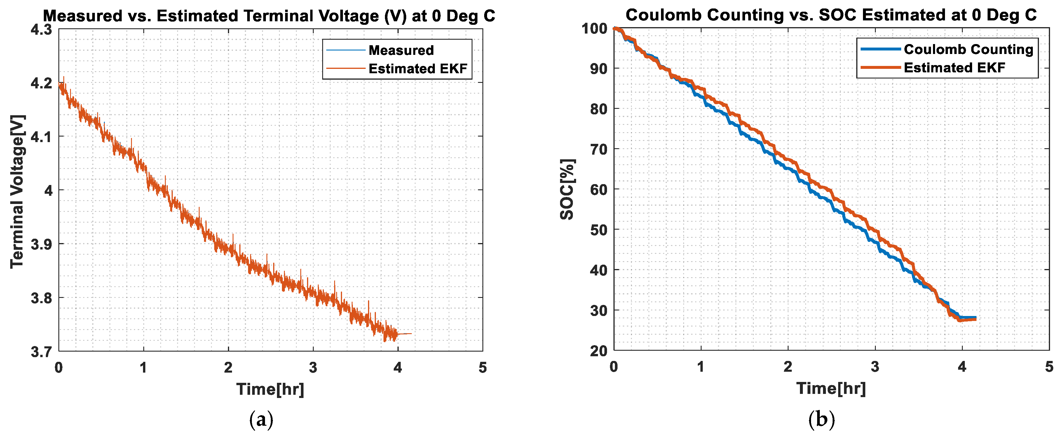
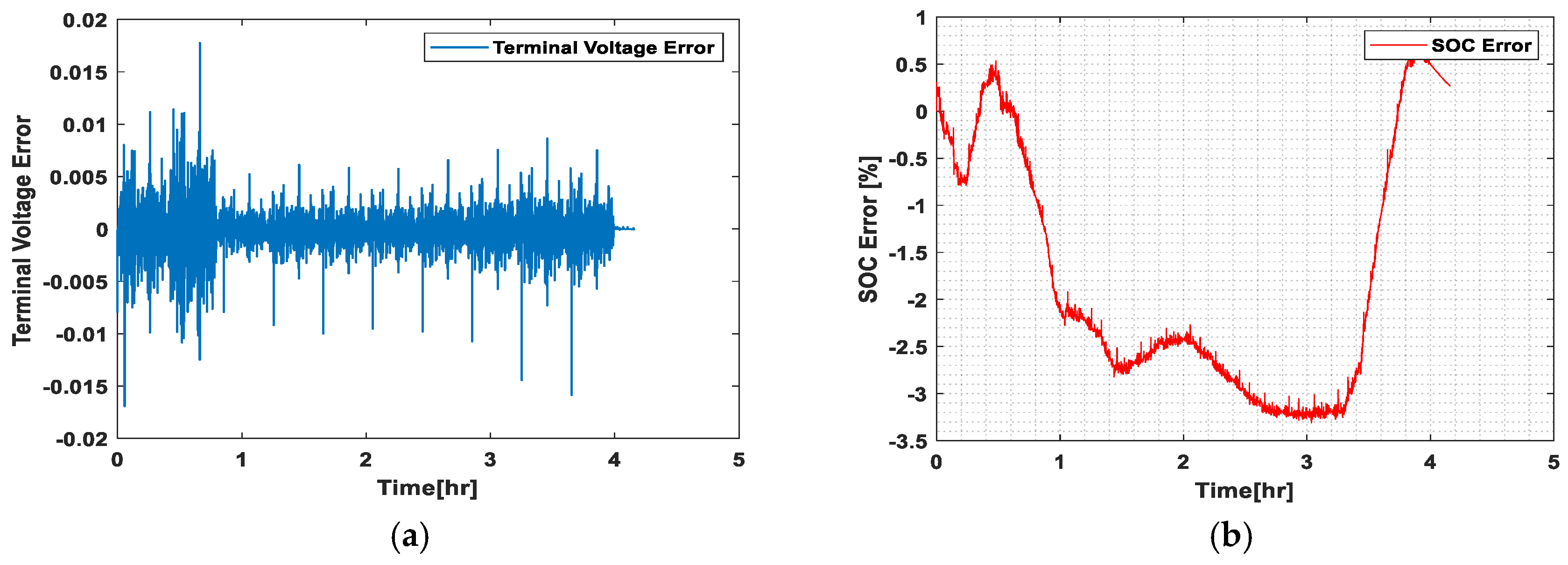
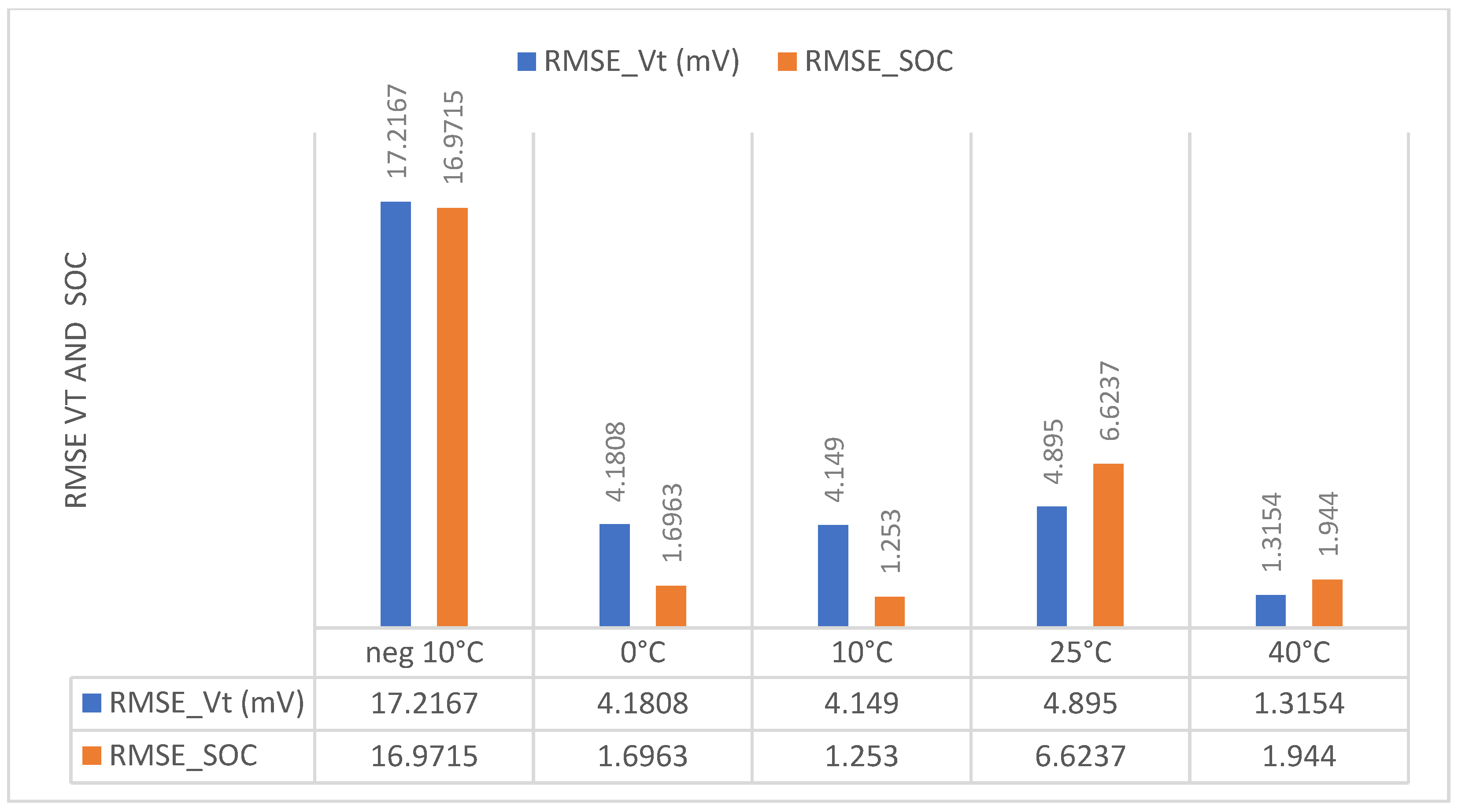
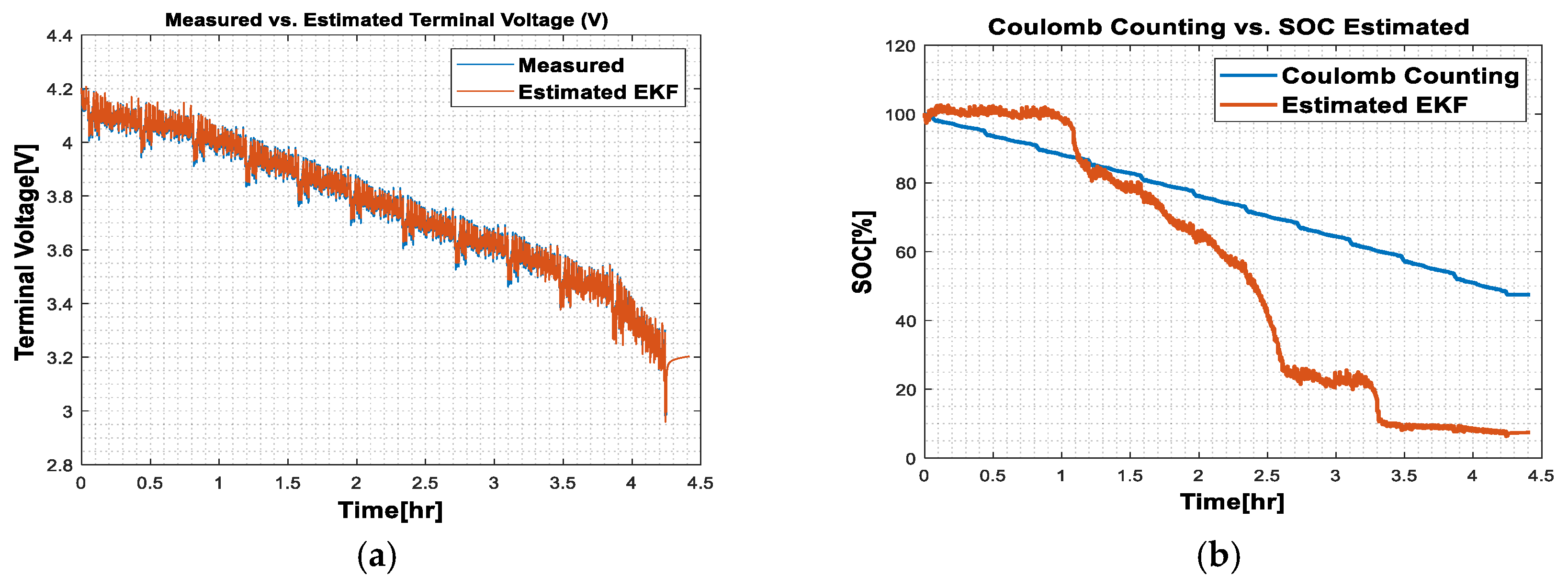
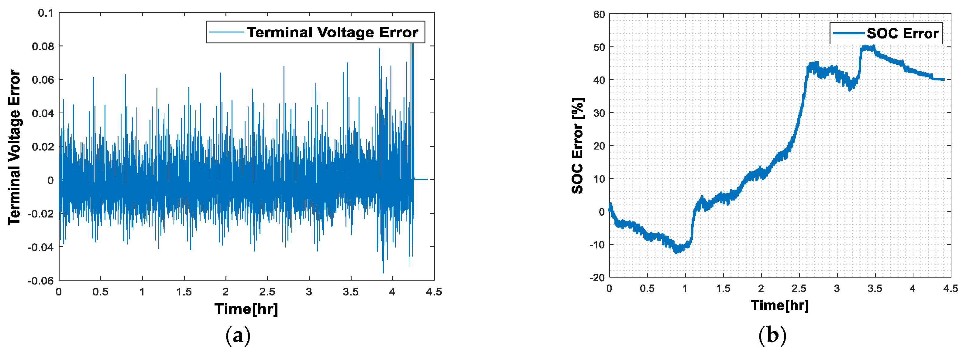
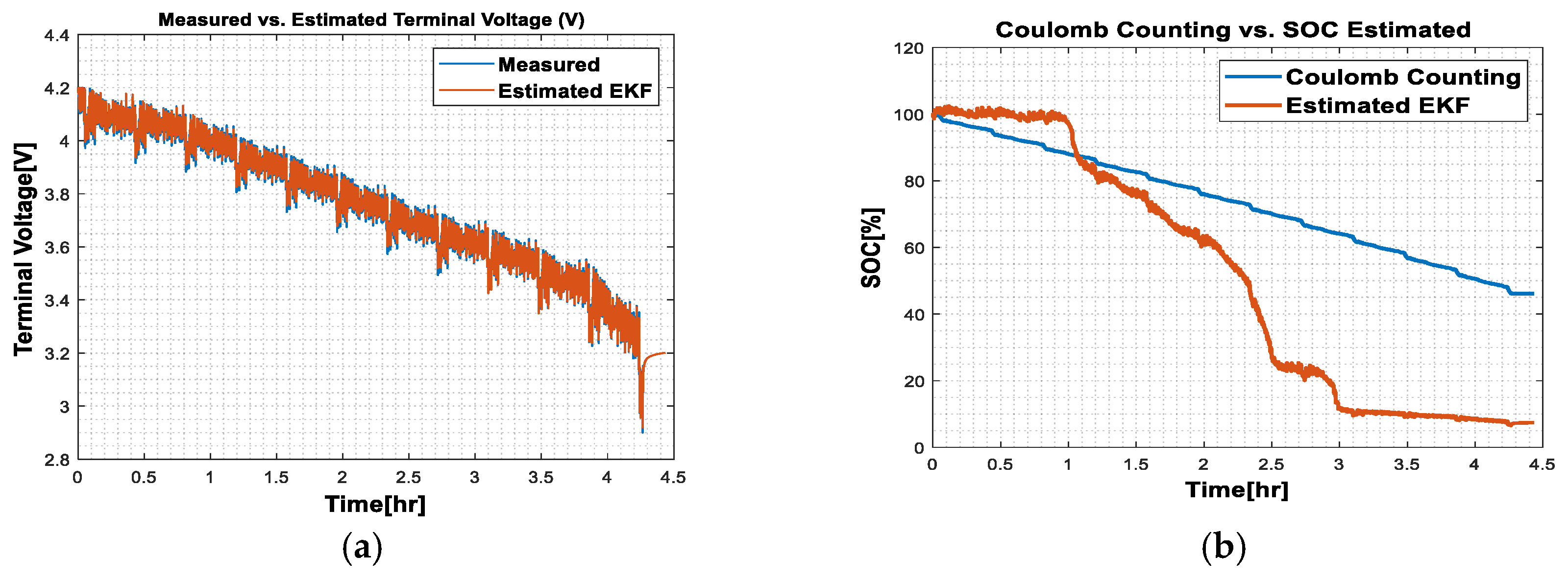
3.1. Results Obtained on the Rotating Graphene Model

(a)

Ambient temperature at 0 °C

Figure 3a,b below illustrates the measured Vt and SOC relative to the LA92 drive cycle estimated at 0 °C.

The SOC-OCV curve and battery model parameters were optimized for each temperature and SOC level from 100% to 0% in 10% increments. The convergence and estimation of SOC and Vt strongly depend on the battery model parameters. The initial P, Q, and R values of the AEKF were manually set so that the average root mean square error (RMSE) of all SOC temperatures was less than 5% and Vt was less than 100 mV. The results of this adjustment can be seen in Figure 4a,b. The RMSE at 40 °C was 1.75% for SOC and 1 mV for Vt for the LA92 drive cycle.

• (b) Ambient temperature at 25 °C

Figure 5a,b below illustrates the measured Vt and SOC relative to the LA92 drive cycle estimated at 25 °C

A bug is observed in the estimation from the 4th hour of testing, due to the double amount of data recorded during the experimental phase and is visible with the appearance of two voltage lines. Nevertheless, this error is taken into account. The convergence of the SOC and Vt towards the predicted values shows good performance of the Extended Adaptive Kalman Filter with minimal RMSE errors. This can be observed in Figure 6a,b.

Figure 7 provides details of the SOC and Vt RMSE under these conditions for all temperatures from −10 °C to 40 °C.

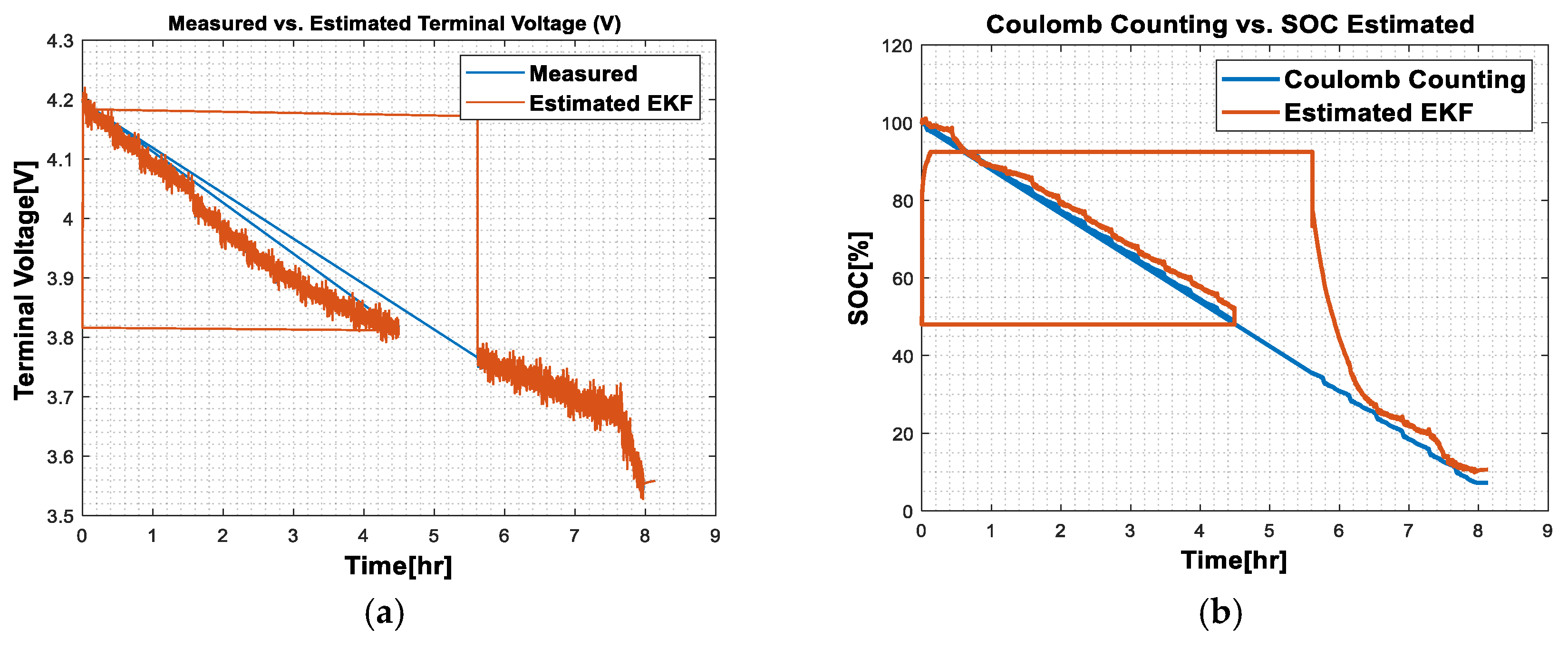
3.2. Results Obtained on the LG 18650HG2 Li-Ion Model

(a)

Ambient temperature at 40 °C

Figure 8a,b below illustrates the measured Vt and SOC against the LG 18650 HG2 drive cycle estimated at 40 °C.

Comparing the estimated voltage values to the experimentally measured values, as well as the state of charge (SOC) values to the values measured using a Coulomb counter at 40 °C, makes it possible to verify the accuracy of the battery models and SOC estimation methods. Given the substantial discrepancy, it appears that the battery model may require adjustments for improved accuracy. Deviations may be due to approximations in the model, unaccounted temperature variations, or complex electrochemical phenomena. A Coulomb counter to measure the SOC of the battery has been used. This device tracks charging and discharging by integrating current over time, giving a direct measurement of SOC.

By analyzing the discrepancies between measured and estimated values, it can be identified where the weak points are in our model or measurement system. Systematic errors may indicate a need for recalibration or modification of the model, while random errors may require accuracy of sensors or data processing algorithms. The estimation errors are presented in Figure 9a,b below:

We find that the SOC estimation error is greater than 50%, which is due to the fact that the values of R, P and Q are static. To improve this result, it would be necessary to recalculate other values, either experimentally or by an optimization algorithm such as particle swarm optimization (PSO), without taking into consideration parameters such as temperature and battery aging.

• (b) Ambient temperature at 25 °C

Figure 10a,b below illustrates the measured Vt and SOC against the LG 18650 HG2 drive cycle estimated at 25 °C.

The estimation errors are presented in Figure 11a,b below:

We notice the SOC estimation error is more than 50% which is due to the fact that the values of R, P, and Q are static. Deviations of more than 50% between the measurement and the SOC setpoint are very significant and cause a serious problem in the Battery Management System (BMS). Here are some possible interpretations:

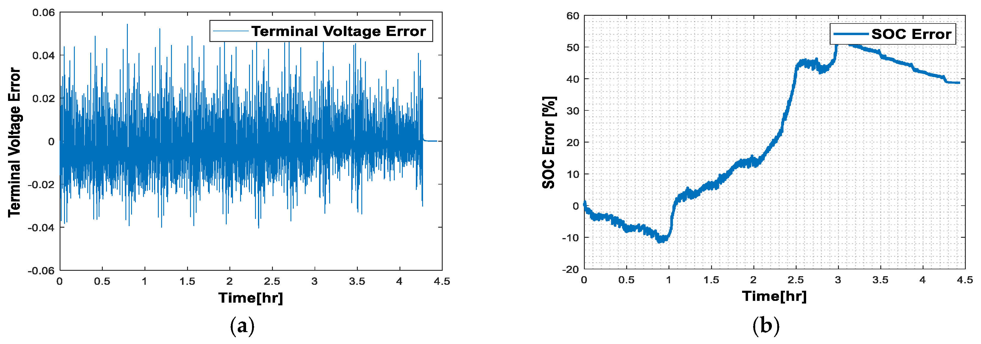
• Risk of Failure: Such a large deviation may indicate that the battery is at risk of failure. This may be due to a severely degraded battery or serious problems in the measurement system.
• Poor Energy Management: Significant errors in the SOC can lead to poor energy management. For example, the battery may be overcharged or discharged excessively, which can shorten its lifespan and affect overall system performance.

The graph below in Figure 12 summarizes the RMSE results obtained for the LG battery model.

The convergence rate and RMSE values of the input error can be improved with more precise tuning values P, Q and R. This histogram allows us to assess the performance of our algorithm on the LG battery model. Ideally, the appropriate temperature level is 40 °C. However, the algorithm can be improved for use over a wider temperature range.

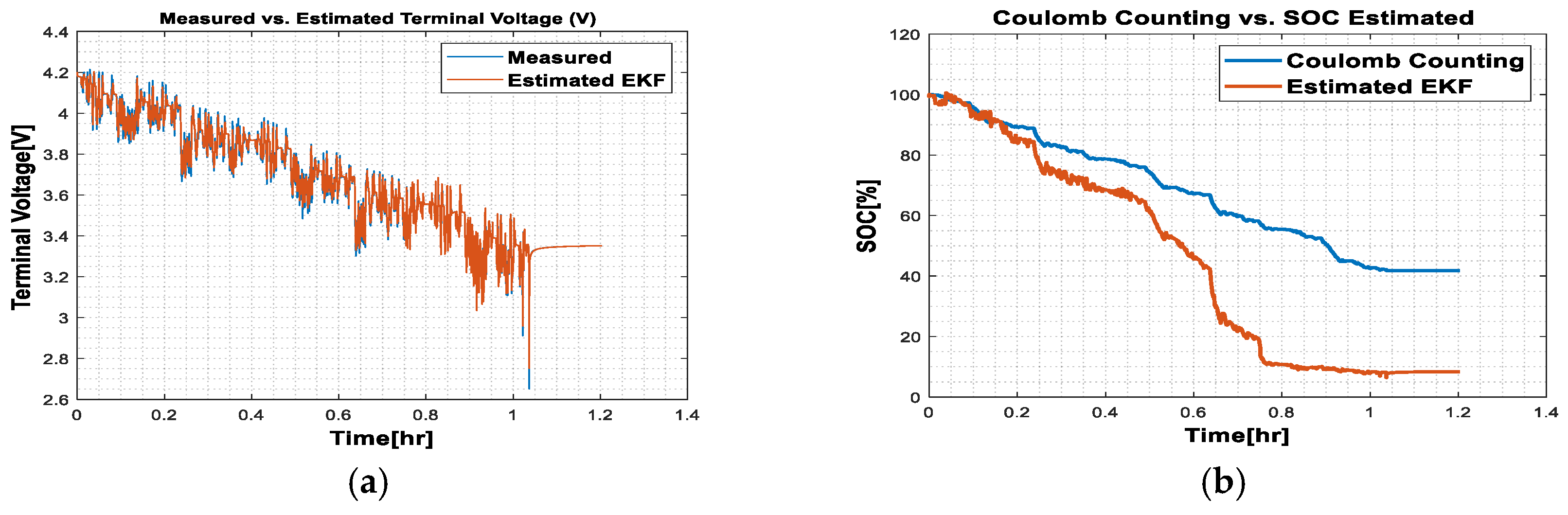
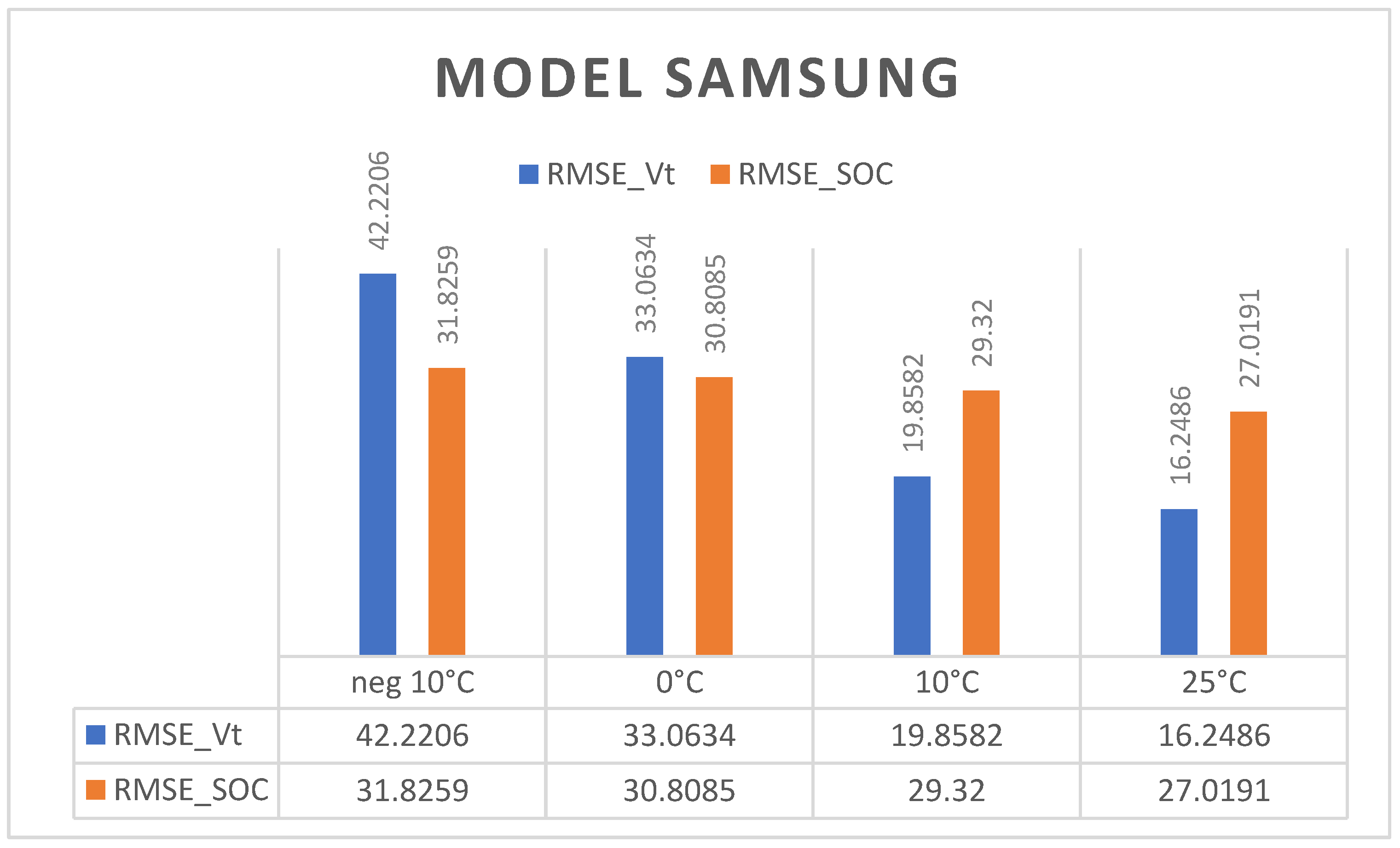
3.3. Results Obtained on the Samsung INR21700 30T Battery Model

• Ambient temperature at 25 °C

Figure 13a,b below illustrates the measured Vt and SOC against the estimated drive cycle of the SAMSUNG INR21700 30T at 25 °C.

The estimation errors are presented in Figure 14a,b below:

The graph in Figure 15 below summarizes the RMSE results obtained for the SAMSUNG battery model.

This histogram in Figure 15 allows us to assess the performance of our algorithm on the Samsung battery model. Ideally, the appropriate temperature level is 25 °C. However, the algorithm can be improved for use over a wider temperature range. The convergence rate and RMSE values of the input error can be improved with more precise tuning values P, Q and R.

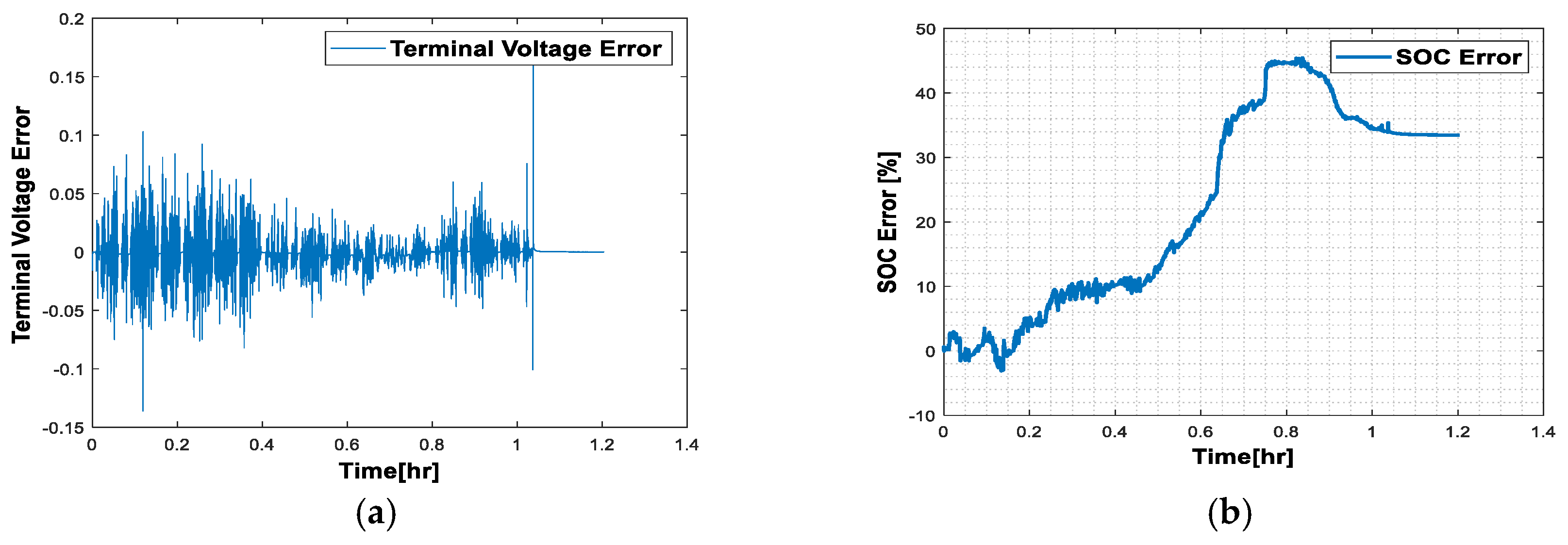
3.4. Results on Battery Model Panasonic 18650pf Li-Ion Battery

• Ambient temperature at 25 °C

Figure 16a,b below illustrates the measured Vt and SOC against the estimated drive cycle of the PANASONIC 18650 PF at 25 °C.

Figure 16a shows the relationship between estimated and experimentally evaluated voltage values. A linear relationship would indicate a good match between the two, while large deviations could indicate errors in the model or measurements. Figure 16b shows the relationship between the SOC values estimated and measured with a Coulomb counter. A linear relationship would indicate good model performance, while significant deviations could indicate errors in SOC estimation or errors in Coulomb counter measurements.

The estimation errors are presented in Figure 17a,b below:

The histogram in Figure 18 summarizes the RMSE values (SOC and OCV) as a function of the different study temperatures. This allows us to analyze the dynamic behavior over time of the state of charge.

3.5. Discussion

Table 4. Summary of results on estimation errors.

Temperature	RMSE (SOC)	RMSE (OCV)
Turnigy graphene
40 °C	1.944	1.3154
25 °C	9.6237	4.895
10 °C	1.253	4.149
0 °C	1.6963	4.1808
−10 °C	16.9715	17.2167
LG
−10 °C	15.3396	33.1543
25 °C	31.4471	8.625
40 °C	29.407	10.727
SAMSUNG
−10 °C	31.8259	42.2206
0 °C	30.8085	33.0634
10 °C	29.32	19.8582
25 °C	27.0191	16.2486
PANASONIC
−10 °C	25.0162	206.7898
0 °C	25.8778	415.1215
10 °C	50.1941	338.5054
25 °C	32.432	248.0957

provides an overall summary of the estimation errors for the four lithium battery manufacturers with the adapted extended Kalman filter algorithm. The various operating scenarios, spanning temperatures from 40 °C to −10 °C, enable comprehensive testing of our algorithm’s performance. This includes adaptive updates of both the process noise covariance and measurement noise covariance, which enhance state of charge estimation accuracy while reducing computational complexity, ensuring high precision and robust stability. Its results comply with ISO 12405-4 and IEC 61982 standards, which respectively address the performance and lifespan requirements of lithium batteries, as well as the safety criteria and testing methods for batteries. This with the following modalities: (a) For performance, batteries must retain at least 90% of their initial capacity after 500 charge and discharge cycles at a temperature of 25 °C. (b) Batteries must be tested at temperatures −20 °C to 40 °C. (c) Batteries must withstand at least 1000 charge and discharge cycles at 25 °C, with an estimated depth of discharge of at least 80%. (d) The error in estimating the state of charge must be less than 5% for lithium-ion batteries.

They are also approved by the work of [1,2], which presents similarities in terms of the speed of convergence of the different estimates. The Turnigy graphene model offers positive results of less than 2% for errors (SOC) in the operating scenarios of 40 °C, 10 °C and 0 °C. The RMSE error is 9.6237% for a temperature of 25 °C, then increases to 16.9715% for a temperature of −10 °C. This observation is also made for the temperature of 40 °C at the level of estimation errors (OCV), which stabilizes at 1.3154%, and for a temperature of 25 °C, the RMSE (OCV) value is 4.895%. We also note that for temperatures of 10 °C, 0 °C, −10 °C, the RMSE (OCV) values are successively 4.149%, 4.1808% and 17.2167%. The errors obtained with the other models are well above the Turnigy graphene model, with a very positive correlation in terms of amplitude and significance, highlighting the specificities of the different technologies used by the different manufacturers. A summary (

Table A1. Comparative mathematical table of different estimation strategies.

Ref	Mathematical Equations	Constraints	Variable Designation
[15]	$\left\{\begin{array}{c}{X}_{K+1=A_x\left(k\right)+B_u\left(k\right)+\mathrm{V}\left(\mathrm{k}\right)}\\ Y_{k+1=C_x\left(k\right)+D_u\left(k\right)+\mathrm{W}\left(\mathrm{k}\right)}\end{array}\right.$	Life extension model = model parameters	The state vector is represented by X(t), the input vector is U(t), while the output vector is Y(t). The system parameters are defined by A, C and B.
[25]	e(k) = z(k) − z (k|k − 1) S(k) = H(k)P(k|k − 1)H(k)T + R(k) K(k) = P(k|k − 1)H(k)TS(k) x(k|k) = x(k|k − 1) + K(k)e(k) P(k|k) = [I − K(k)H(k)]P(k|k − 1)	Residual capacity model = load variables	The measurement z(k), innovation e(k), predicted value Z(k|k − 1), the estimate of the state x(k|k), associated covariance matrix P(k|k)
[26]	$E_0$ − ${\displaystyle \frac{\mathrm{K}Q}{Q-it}}\mathrm{A}{e}^{-B.it}$	Long-term estimation model = variables	K, the polarization constant expressed in V, Q the capacity of the battery expressed in Ah, A the amplitude of the exponential zone expressed in V, B a constant expressed in A-1h-1, it the current charge of the battery, E0 the constant voltage of the battery,
[29]	yk = E0 − Rik − Ki/SoC y = E0 − Rik + K2ln(SoC) + K4ln(1 − SoC)	Aging model = aging variables	E0 is the DC compensation; Rik is the internal resistance; ik is the current; Kx and the constants are used to adjust the curve
[18]	y(k) = θ(k)Tφ(k) K0 = ${\displaystyle \frac{P0(k-1)\phi \left(k\right)}{1+\phi \left(k\right)TP0(k-1)\phi \left(k\right)}}$ P0(k) = [I − K0φ(k)T]P0(k − 1)	Impact of temperature = temperature	Vb: main branch voltage (V), Erno: open circuit voltage at full load (V), Ko: constant (V 1 °C); e: internal temperature (OK) RD: resistance at the battery terminals (n), Roo: constant resistance (n),
[19]	yk + 1 = Akyk + Bkuk + Γkξk; wk = Ckyk + Dkuk + ηk, xk + 1 = Akxk + Γkξk vk = Ckxk + ηk	Cycle optimization = charge cycles	yk is the n-state vector of the process. Ak is the (n,n)-deterministic state transition matrix, uk is the deterministic ordering m-vector, Bk is the deterministic (n,m)-matrix which connects the command uk to the state yk + 1, ξk is the p-vector of white noise, which models the error of the process, with a mean and a known (p,p)-covariance variance matrix Qk, Γk is the deterministic (n,p)-matrix which connects the white noise ξk to the state yk + 1, wk is the observation q-vector
[20]	E = E0 − k Q Q − it + Aexp (−B.it)	Experimental validation = experimental data	E is the no-load voltage (V) E0 is the constant battery voltage (V) K is the bias voltage (V) Q is the battery capacity (Ah) This is the current battery charge (Ah) A is the amplitude of the exponential zone (V) B is the inverse of the time constant of the exponential zone (Ah)-1.
[21]	$X^{°}$ = F(x,u) w y = G(x,u) v	Precision = comparative methods	X the SOC; w represents errors due to external disturbances as well as modeling errors, v represents the measurement errors.

) in Appendix A with several mathematical models has been proposed with the aim of making a better comparison with the hybrid method developed in this work. In addition, the results obtained in this article are also highlighted in the work [55], which addresses a direct application of the state of charge SOC of a supercapacitor of a Railway Power Conditioner (RDPC). And therefore, the main role is to compensate the normal reverse currents (NSC), but also to reduce the impact of power fluctuations caused by braking or starting the locomotive on the electrical network. The balancing control methods are therefore developed for the voltages of the capacitors of the sub-modules (SM) and the state of charge (SOC) of the supercapacitor, which are associated with the operating modes. The SOC estimate for this battery in the above-mentioned work reaches 50% for a completion time of 500 ms, with inflection points at times t1 = 170 ms and t2 = 330 ms.

This approach is consistent with the results obtained in our article for:

(a) The cases of SOC estimation of the studied batteries that are greater than 50% for a duration of 0.00069 (s). This rapid convergence obtained in our results is therefore justifiable based on the above.

(b) Optimal noise suppression and better temporal control of the covariance matrix in the process of estimating the battery SOC provides a state of charge estimation error of less than 2%.

These results are also confirmed by the work [56], which proposes a model-free deep reinforcement learning (DRL) method. The DRL-based energy management system (EMS) is tested on the OPAL-RT experimental platform using field charging data. Case studies have demonstrated that the proposed method outperforms traditional rule-based and optimization methods by more than 5% in terms of energy management.

4. Conclusions

In this article, it is proposed an adaptive extended Kalman filter (AEKF) algorithm designed to accurately estimate dynamic parameters, such as the state of charge (SOC), across four different lithium battery models (Turnigy, LG, SAMSUNG, PANASONIC) for temperatures 40 °C, 25 °C, 10 °C, 0 °C and −10 °C. The main contributions in this work were as follows:

(a) Optimal noise suppression and better temporal control of the covariance matrix in the battery SOC estimation process.

(b) The precise knowledge of the system model and the dynamics of its parameters with an iterative method integrating the second-order Taylor development, which combines the proposal of an estimator applied to a first-order Thévenin model to strengthen the robustness and accuracy of the system parameters. This methodological mixture makes it possible to resolve the limitations developed by [1,42].

(c) Providing simulation conditions that closely resemble industrial realities, as the parameter estimations at the base differ significantly across various battery technologies. This variability arises because the collected and estimated data fluctuate substantially depending on the online experimental conditions employed by different manufacturers, despite the technical operating characteristics of the batteries remaining within similar ranges. This reality makes the simulation protocol very stochastic, hence the challenge of this study, which highlights the chaotic fluctuations in the estimation and validation of the models by stability margins.

(d) A comprehensive comparison and classification of estimation methods in the context of implementing the adaptive Kalman algorithm, as documented in current literature, is achieved through a rigorous mathematical analysis of analytical models that incorporate various constraints. This approach not only enhances existing methods by highlighting their respective strengths and weaknesses but also provides deeper insights into their methodological differences. Ultimately, the goal is to improve overall performance in a manner conducive to the sustainable development of the automotive sector.

The results obtained were mapped charging status (SOC) versus open circuit voltage (OCV), and the high-performance primitive collection (HPPC) tests were carried out at 40 °C, 25 °C, 10 °C, 0 °C and −10 °C. At these temperatures, their corresponding values for the root mean square error (RMSE) of (SOC) for the Turnigy graphene battery model were found to be: 1.944, 9.6237, 1.253, 1.6963, 16.9715, and for (OCV): 1.3154, 4.895, 4.149, 4.1808, and 17.2167, respectively.

From the perspective of this work, it becomes necessary to propose an intelligent method of optimization of the parameters P, Q and R for an in-depth comparative study of the different dynamic operating scenarios according to the technologies used by lithium battery manufacturers. This will allow the development of new generations of even more efficient batteries offering a better lifespan. The impact of battery aging will also be taken into account for the continuation of the work.

References

1. Bockrath, S.; Lorentz, V.; Pruckner, M. State of health estimation of lithium-ion batteries with a temporal convolutional neural network using partial load profiles. Appl. Energy 2023, 329, 120307. [Google Scholar] [CrossRef]
2. Zheng, L.; Zhu, J.; Lu, D.D.-C.; Wang, G.; He, T. Incremental capacity analysis and differential voltage analysis based state of charge and capacity estimation for lithium-ion batteries. Energy 2018, 150, 759–769. [Google Scholar] [CrossRef]
3. Liu, Y.; Huang, Z.; Wu, Y.; Yan, L.; Jiang, F.; Peng, J. An online hybrid estimation method for the core temperature of Lithium-ion battery with model noise compensation. Appl. Energy 2022, 327, 120037. [Google Scholar] [CrossRef]
4. Sun, L.; Li, G.; You, F. Combined internal resistance and state-of-charge estimation of lithium-ion battery based on extended state observer. Renew. Sustain. Energy Rev. 2020, 131, 109994. [Google Scholar] [CrossRef]
5. Gong, D.; Gao, Y.; Kou, Y.; Wang, Y. State of health estimation for lithium-ion battery based on energy features. Energy 2022, 257, 124812. [Google Scholar] [CrossRef]
6. Yang, Y.; Bremner, S.; Menictas, C.; Kay, M. Battery energy storage system size determination in renewable energy systems: A review. Renew. Sustain. Energy Rev. 2018, 91, 109–125. [Google Scholar] [CrossRef]
7. Jiang, Y.; Chen, Y.; Yang, F.; Peng, W. State of health estimation of lithium-ion battery with automatic feature extraction and self-attention learning mechanism. J. Power Sources 2023, 556, 232466. [Google Scholar] [CrossRef]
8. Apostolou, D.; Xydis, G. A literature review on hydrogen refuelling stations and infrastructure. Current status and future prospects. Renew. Sustain. Energy Rev. 2019, 113, 109292. [Google Scholar] [CrossRef]
9. Hu, Y.; Zhang, Y.; Wang, S.; Xu, W.; Fan, Y.; Liu, Y. Joint dynamic strategy of Bayesian regularized back propagation neural network with strong robustness—Extended Kalman filtering for the battery state-of-charge prediction. Int. J. Electrochem. Sci. 2021, 16, 21118. [Google Scholar] [CrossRef]
10. Li, Z.; Zhang, C.; Han, F.; Zhang, F.; Zhou, D.; Xu, S.; Liu, H.; Li, X.; Liu, J. Improving the cycle stability of FeCl3-graphite intercalation compounds by polar Fe2O3 trapping in lithium-ion batteries. Nano Res. 2019, 12, 1836–1844. [Google Scholar] [CrossRef]
11. Li, Z.; Zhang, C.; Han, F.; Wang, F.; Zhang, F.; Shen, W.; Ye, C.; Li, X.; Liu, J. Towards high-volumetric performance of Na/Li-ion batteries: A better anode material with molybdenum pentachloride—Graphite intercalation compounds (MoCl5–GICs). J. Mater. Chem. A 2020, 8, 2430–2438. [Google Scholar] [CrossRef]
12. Tong, J.; Xiao, X.; Liang, X.; von Solms, N.; Huo, F.; He, H.; Zhang, S. Insights into the solvation and dynamic behaviors of a lithium salt in organic- and ionic liquid-based electrolytes. Phys. Chem. Chem. Phys. 2019, 21, 19216–19225. [Google Scholar] [CrossRef]
13. Tan, X.F.; McDonald, S.D.; Gu, Q.; Hu, Y.; Wang, L.; Matsumura, S.; Nishimura, T.; Nogita, K. Characterisation of lithium-ion battery anodes fabricated via in-situ Cu6Sn5 growth on a copper current collector. J. Power Sources 2019, 415, 50–61. [Google Scholar] [CrossRef]
14. Philippe, B. Etude D’interfaces Électrode/Électrolyte Dans Des Batteries Li-ion par Spectroscopie Photoélectronique à Différentes Profondeurs. Ph.D. Thesis, Université de Pau et des Pays de l’Adour, Pau, France, 2013. [Google Scholar]
15. Peng, J.; Luo, J.; He, H.; Lu, B. An improved state of charge estimation method based on cubature Kalman filter for lithium-ion batteries. Appl. Energy 2019, 253, 113520. [Google Scholar] [CrossRef]
16. Pastor-Fernández, C.; Yu, T.F.; Widanage, W.D.; Marco, J. Critical review of non-invasive diagnosis techniques for quantification of degradation modes in lithium-ion batteries. Renew. Sustain. Energy Rev. 2019, 109, 138–159. [Google Scholar] [CrossRef]
17. Mouodo, L.V.A.; Ali, A.-H.M.; Tamba, J.G.; Olivier, T.S.M. Comparison and classification of six reference currents extraction algorithms for harmonic compensation on a stochastic power network: Case of the TLC hybrid filter. Cogent Eng. 2022, 9, 2076322. [Google Scholar] [CrossRef]
18. Chen, S.; Wen, H.; Wu, J.; Lei, W.; Hou, W.; Liu, W.; Xu, A.; Jiang, Y. Internet of Things Based Smart Grids Supported by Intelligent Edge Computing. IEEE Access 2019, 7, 74089–74102. [Google Scholar] [CrossRef]
19. Chen, Z.P.; Wang, Q.T. The Application of UKF Algorithm for 18650-type Lithium Battery SOH Estimation. Appl. Mech. Mater. 2014, 519, 1079–1084. [Google Scholar] [CrossRef]
20. Chen, Z.; Mi, C.C.; Fu, Y.; Xu, J.; Gong, X. Online battery state of health estimation based on Genetic Algorithm for electric and hybrid vehicle applications. J. Power Sources 2013, 240, 184–192. [Google Scholar] [CrossRef]
21. Mouodo, L.V.A.; Ali, A.-H.M.; Mayi, O.T.S.; Tamba, J.G.; Axaopoulos, P. Recent Progress and Challenges of Algorithms for Reducing Power Losses and Optimal Reconfiguration of Voltage Profiles for Distribution Networks. Int. J. Electron. Commun. Eng. 2024, 11, 176–194. [Google Scholar] [CrossRef]
22. Chikkannanavar, S.B.; Bernardi, D.M.; Liu, L. A review of blended cathode materials for use in Li-ion batteries. J. Power Sources 2014, 248, 91–100. [Google Scholar] [CrossRef]
23. Cleary, B.; Duffy, A.; O’Connor, A.; Conlon, M.; Fthenakis, V.; Oconnor, A. Assessing the Economic Benefits of Compressed Air Energy Storage for Mitigating Wind Curtailment. IEEE Trans. Sustain. Energy 2015, 6, 1021–1028. [Google Scholar] [CrossRef]
24. Cui, Y.; Zuo, P.; Du, C.; Gao, Y.; Yang, J.; Cheng, X.; Ma, Y.; Yin, G. State of health diagnosis model for lithium ion batteries based on real-time impedance and open circuit voltage parameters identification method. Energy 2018, 144, 647–656. [Google Scholar] [CrossRef]
25. Xia, B.; Chen, C.; Tian, Y.; Wang, M.; Sun, W.; Xu, Z. State of charge estimation of lithium-ion batteries based on an improved parameter identification method. Energy 2015, 90, 1426–1434. [Google Scholar] [CrossRef]
26. Ng, K.S.; Moo, C.-S.; Chen, Y.-P.; Hsieh, Y.-C. Enhanced coulomb counting method for estimating state-of-charge and state-of-health of lithium-ion batteries. Appl. Energy 2009, 86, 1506–1511. [Google Scholar] [CrossRef]
27. Yang, N.; Zhang, X.; Li, G. State of charge estimation for pulse discharge of a LiFePO4 battery by a revised Ah counting. Electrochim. Acta 2015, 151, 63–71. [Google Scholar] [CrossRef]
28. Yang, R.; Xiong, R.; He, H.; Mu, H.; Wang, C. A novel method on estimating the degradation and state of charge of lithium-ion batteries used for electrical vehicles. Appl. Energy 2017, 207, 336–345. [Google Scholar] [CrossRef]
29. Mouodo, L.V.A.; Ali, A.-H.M.; Thierry, S.M.O.; Moteyo, A.D.; Tamba, J.G.; Axaopoulos, P. Comparison and classification of photovoltaic system architectures for limiting the impact of the partial shading phenomenon. Heliyon 2024, 10, e36670. [Google Scholar] [CrossRef]
30. Yang, F.; Li, W.; Li, C.; Miao, Q. State-of-charge estimation of lithium-ion batteries based on gated recurrent neural network. Energy 2019, 175, 66–75. [Google Scholar] [CrossRef]
31. Tang, X.; Gao, F.; Zou, C.; Yao, K.; Hu, W.; Wik, T. Load-responsive model switching estimation for state of charge of lithium-ion batteries. Appl. Energy 2019, 238, 423–434. [Google Scholar] [CrossRef]
32. Li, Y.; Wang, C.; Gong, J. A multi-model probability SOC fusion estimation approach using an improved adaptive unscented Kalman filter technique. Energy 2017, 141, 1402–1415. [Google Scholar] [CrossRef]
33. Shen, Y. Improved chaos genetic algorithm based state of charge determination for lithium batteries in electric vehicles. Energy 2018, 152, 576–585. [Google Scholar] [CrossRef]
34. Zheng, F.; Xing, Y.; Jiang, J.; Sun, B.; Kim, J.; Pecht, M. Influence of different open circuit voltage tests on state of charge online estimation for lithium-ion batteries. Appl. Energy 2016, 183, 513–525. [Google Scholar] [CrossRef]
35. Huang, F.; Ma, J.; Xia, H.; Huang, Y.; Zhao, L.; Su, S.; Kang, F.; He, Y.-B. Capacity Loss Mechanism of the Li4Ti5O12 Microsphere Anode of Lithium-Ion Batteries at High Tem-perature and Rate Cycling Conditions. ACS Appl. Mater. Interfaces 2019, 11, 37357–37364. [Google Scholar] [CrossRef]
36. Dey, S.; Ayalew, B.; Pisu, P. Combined estimation of State-of-Charge and State-of-Health of Li-ion battery cells using SMO on electrochemical model. In Proceedings of the 2014 13th International Workshop on Variable Structure Systems (VSS), Nantes, France, 29 June–2 July 2014; pp. 1–6, ISSN 2158-3986. [Google Scholar]
37. Dimitrov, R.S. The Paris Agreement on Climate Change: Behind Closed Doors. Glob. Environ. Politics 2016, 16, 1–11. [Google Scholar] [CrossRef]
38. Zhang, X.; Gao, X.; Duan, L.; Gong, Q.; Wang, Y.; Ao, X. A novel method for state of health estimation of lithium-ion batteries based on fractional-order differential voltage-capacity curve. Appl. Energy 2024, 377 Pt 2, 124404. [Google Scholar] [CrossRef]
39. Yang, F.; Zhang, S.; Li, W.; Miao, Q. State-of-charge estimation of lithium-ion batteries using LSTM and UKF. Energy 2020, 201, 117664. [Google Scholar] [CrossRef]
40. Sheng, H.; Xiao, J. Electric vehicle state of charge estimation: Nonlinear correlation and fuzzy support vector machine. J. Power Sources 2015, 281, 131–137. [Google Scholar] [CrossRef]
41. Zahid, T.; Xu, K.; Li, W.; Li, C.; Li, H. State of charge estimation for electric vehicle power battery using advanced machine learning algorithm under diversified drive cycles. Energy 2018, 162, 871–882. [Google Scholar] [CrossRef]
42. Alsuwian, T.; Ansari, S.; Zainuri, M.A.A.M.; Ayob, A.; Hussain, A.; Lipu, M.H.; Alhawari, A.R.; Almawgani, A.; Almasabi, S.; Hindi, A.T. A review of expert hybrid and co-estimation techniques for SOH and RUL estimation in battery management system with electric vehicle application. Expert Syst. Appl. 2024, 246, 123123. [Google Scholar] [CrossRef]
43. Ali, A.M.; Mouodo, L.V.A.; Patrice, N.N.T.; Tamba, J.G.; Axaopoulos, P. Simulation and Innovative Digital Modeling Approach for Improving the Dynamic Performances of HVDC MMC Systems: Case of an AVM-MMC Migration. Int. J. Electron. Commun. Eng. 2024, 11, 77–90. [Google Scholar] [CrossRef]
44. Chemali, E.; Kollmeyer, P.J.; Preindl, M.; Emadi, A. State-of-charge estimation of Li-ion batteries using deep neural networks: A machine learning approach. J. Power Sources 2018, 400, 242–255. [Google Scholar] [CrossRef]
45. Mouodo, L.V.A.; Ali, A.-H.M.; Tamba, J.G.; Olivier, T.S.M. Experimental Characterization of Reference Currents for Harmonic Compensation: Case of the TLC Hybrid Filter. Int. Rev. Electr. Eng. 2024, 19, 40. [Google Scholar] [CrossRef]
46. Tian, Y.; Lai, R.; Li, X.; Xiang, L.; Tian, J. A combined method for state-of-charge estimation for lithium-ion batteries using a long short-term memory network and an adaptive cubature Kalman filter. Appl. Energy 2020, 265, 114789. [Google Scholar] [CrossRef]
47. Cui, Z.; Dai, J.; Sun, J.; Li, D.; Wang, L.; Wang, K.; Pereira, A.M.B. Hybrid Methods Using Neural Network and Kalman Filter for the State of Charge Estimation of Lithium-Ion Battery. Math. Probl. Eng. 2022, 2022, 9616124. [Google Scholar] [CrossRef]
48. Bian, C.; He, H.; Yang, S. Stacked bidirectional long short-term memory networks for state-of-charge estimation of lithium-ion batteries. Energy 2020, 191, 116538. [Google Scholar] [CrossRef]
49. Tang, X.; Liu, B.; Lv, Z.; Gao, F. Observer based battery SOC estimation: Using multi-gain-switching approach. Appl. Energy 2017, 204, 1275–1283. [Google Scholar] [CrossRef]
50. Dai, H.; Guo, P.; Wei, X.; Sun, Z.; Wang, J. ANFIS (adaptive neuro-fuzzy inference system) based online SOC (State of Charge) correction considering cell divergence for the EV (electric vehicle) traction batteries. Energy 2015, 80, 350–360. [Google Scholar] [CrossRef]
51. Dong, X.; Zhang, C.; Jiang, J. Evaluation of SOC Estimation Method Based on EKF/AEKF under Noise Interference. Energy Procedia 2018, 152, 520–525. [Google Scholar] [CrossRef]
52. Sun, D.; Yu, X.; Wang, C.; Zhang, C.; Huang, R.; Zhou, Q.; Amietszajew, T.; Bhagat, R. State of charge estimation for lithium-ion battery based on an Intelligent Adaptive Extended Kalman Filter with improved noise estimator. Energy 2021, 214, 119025. [Google Scholar] [CrossRef]
53. Zhai, X.; Li, Z.; Li, Z.; Xue, Y.; Chang, X.; Su, J.; Jin, X.; Wang, P.; Sun, H. Risk-averse energy management for integrated electricity and heat systems considering building heating vertical imbalance: An asynchronous decentralized approach. Appl. Energy 2025, 383, 125271. [Google Scholar] [CrossRef]
54. Ding, B.; Li, Z.; Li, Z.; Xue, Y.; Chang, X.; Su, J.; Sun, H. Cooperative Operation for Multiagent Energy Systems Integrated with Wind, Hydrogen, and Buildings: An Asymmetric Nash Bargaining Approach. IEEE Trans. Ind. Inform. 2025. [Google Scholar] [CrossRef]
55. Guo, P.; Xu, Q.; Yue, Y.; Ma, F.; He, Z.; Luo, A.; Guerrero, J.M. Analysis and Control of Modular Multilevel Converter with Split Energy Storage for Railway Traction Power Conditioner. IEEE Trans. Power Electron. 2020, 35, 1239–1255. [Google Scholar] [CrossRef]
56. Chen, J.; Zhao, Y.; Wang, M.; Yang, K.; Ge, Y.; Wang, K.; Lin, H.; Pan, P.; Hu, H.; He, Z.; et al. Multi-Timescale Reward-Based DRL Energy Management for Regenerative Braking Energy Storage System. IEEE Trans. Transp. Electrif. 2025, 11, 7488–7500. [Google Scholar] [CrossRef]
Figure 1. (A) First-order Thevenin equivalent circuit model. (B) Flowchart of the proposed method.
Energies 18 03436 g001
Figure 2. (a) Discharge resistance versus SOC of a Turnigy Graphene 5000 mAh Li-ion battery and (b) different temperatures and the characteristics of a Turnigy Graphene 5000 mAh Li-ion battery at Different temperatures.
Energies 18 03436 g002
Figure 3. (a) Estimated voltage value relative to the experimentally measured value, (b) the estimated SOC value relative to the value measured with the Coulomb counter at 0 °C.
Energies 18 03436 g003
Figure 4. Determination of deviations (errors) between measurement and setpoint. (a) Terminal Voltage; (b) SOC.
Energies 18 03436 g004
Figure 5. (a) Estimated voltage value versus experimentally measured value, (b) estimated SOC value versus measured value with Coulomb counter at 25 °C.
Energies 18 03436 g005
Figure 6. Determination of deviations (errors) between measurement and setpoint. (a) Terminal Voltage; (b) SOC.
Energies 18 03436 g006
Figure 7. RMSE error of SOC and Vt at different temperatures for the driving cycle of the LA92 from the manufacturer, Graphene Turnigy.
Energies 18 03436 g007
Figure 8. (a) Estimated voltage value versus experimentally measured value, (b) estimated SOC value versus value measured with a Coulomb counter at 40 °C.
Energies 18 03436 g008
Figure 9. Determination of deviations (errors) between measurement and setpoint at 40 °C. (a) Terminal Voltage; (b) SOC.
Energies 18 03436 g009
Figure 10. (a) Estimated voltage value versus experimentally measured value, (b) Estimated SOC value versus value measured with a Coulomb counter at 25 °C.
Energies 18 03436 g010
Figure 11. Determination of the differences (errors) between the measurement and the setpoint at 25 °C. (a) Terminal Voltage; (b) SOC.
Energies 18 03436 g011
Figure 12. Histogram of RMSE of the LG model.
Energies 18 03436 g012
Figure 13. (a) Estimated voltage value versus experimentally measured value, (b) estimated SOC value versus measured value with Coulomb counter at 25 °C.
Energies 18 03436 g013
Figure 14. Determination of the differences (errors) between the measurement and the setpoint at 25 °C. (a) Terminal Voltage; (b) SOC.
Energies 18 03436 g014
Figure 15. Histogram of RMSE of the SAMSUNG model.
Energies 18 03436 g015
Figure 16. (a) Voltage value evaluated with respect to the experimentally measured value, (b) the SOC value increased with respect to the value measured with the Coulomb counter at 25 °C.
Energies 18 03436 g016
Figure 17. Determination of deviations (errors) between measurement and setpoint at 25 °C. (a) Terminal Voltage; (b) SOC.
Energies 18 03436 g017
Figure 18. Histogram of RMSE for the PANASONIC model.
Energies 18 03436 g018