Article

Neural ODE-Based Dynamic Modeling and Predictive Control for Power Regulation in Distribution Networks

1
Electric Power Research Institute of Guangxi Power Grid Co., Ltd., Nanning 530032, China
2
Guangxi Key Laboratory of Intelligent Control and Maintenance of Power Equipment, Nanning 530032, China
3
State Key Laboratory of Power System Operation and Control, Department of Electrical Engineering, Tsinghua University, Beijing 100084, China
*
Author to whom correspondence should be addressed.
Energies 2025, 18(13), 3419; https://doi.org/10.3390/en18133419
Submission received: 4 June 2025 / Revised: 23 June 2025 / Accepted: 25 June 2025 / Published: 29 June 2025

Abstract

The increasing penetration of distributed energy resources (DERs) and power electronic loads challenges the modeling and control of modern distribution networks (DNs). The traditional models often fail to capture the complex aggregate dynamics required for advanced control strategies. This paper proposes a novel framework for DN power regulation based on Neural Ordinary Differential Equations (NODEs) and Model Predictive Control (MPC). NODEs are employed to develop a data-driven, continuous-time dynamic model capturing the aggregate relationship between the voltage at the point of common coupling (PCC) and the network’s power consumption, using only PCC measurements. Building upon this NODE model, an MPC strategy is designed to regulate the DN’s active power by manipulating the PCC voltage. To ensure computational tractability for real-time applications, a local linearization technique is applied to the NODE dynamics within the MPC, transforming the optimization problem into a standard Quadratic Programming (QP) problem that can be solved efficiently. The framework’s efficacy is comprehensively validated through simulations. The NODE model demonstrates high accuracy in predicting the dynamic behavior in a DN against a detailed simulator, with maximum relative errors below 0.35% for active power. The linearized NODE-MPC controller shows effective tracking performance, constraint handling, and computational efficiency, with typical QP solve times below 0.1 s within a 0.1 s control interval. The validation includes offline tests using the NODE model and online co-simulation studies using CloudPSS and Python via Redis. Application scenarios, including Conservation Voltage Reduction (CVR) and supply–demand balancing, further illustrate the practical potential of the proposed approach for enhancing the operation and efficiency of modern distribution networks.

1. Introduction

1.1. The Background and Motivation

Power distribution networks (DNs) are undergoing a profound transformation, evolving from passive conduits delivering power unidirectionally to active systems integrating significant amounts of distributed energy resources (DERs), such as photovoltaic (PV) generation, and supplying increasingly complex loads, including to electric vehicles and power electronic devices [1]. This paradigm shift introduces bidirectional power flows, increased variability, and complex non-linear behaviors, significantly increasing the operational complexity of DNs [2]. Secure and stable operation of the power system faces substantial challenges due to the growing proportion of variable renewable energy generation [2]. To address this, control of the active power consumption within DNs, often achievable through voltage regulation at the point of common coupling (PCC), is becoming a critical strategy for ensuring supply–demand balance, enabling peak shaving, and improving the energy efficiency through initiatives like Conservation Voltage Reduction (CVR) [3,4].
The effective implementation of such advanced control strategies necessitates accurate dynamic models of the DN. Traditional modeling approaches, often relying on static representations like the ZIP model or component-based dynamic models (e.g., ZIP+IM), struggle to accurately capture the aggregate dynamic response of these modern, heterogeneous networks [5,6]. These models typically require detailed knowledge of the network topology and component parameters, which may be unavailable or inaccurate, and aggregation methods may oversimplify the interactions between diverse elements [7]. The increasing penetration of components like PV systems further complicates the applicability of fixed-structure models [7]. Therefore, there is a critical need for advanced, data-driven modeling techniques that can accurately represent the dynamic behavior of complex DNs based on the operational data observed at the PCC.
This paper presents a framework addressing the challenge of modeling and controlling modern DNs by proposing a data-driven approach based on Neural Ordinary Differential Equations (NODEs) integrated with Model Predictive Control (MPC).

1.2. The Literature Review

The challenge of modeling and controlling DNs has been addressed using various approaches.

1.2.1. Distribution Network Modeling

Physics-based or gray-box models, such as the widely used ZIP+IM structure, attempt to represent the network using equivalent circuits derived from physical principles combined with parameter estimation from measurements [5,6,8,9]. While they provide some physical interpretability, these methods face difficulties due to the complexity of modern networks, the large number of parameters required, and the potential unavailability of detailed system information. For instance, aggregating diverse load types into a single equivalent ZIP+IM model requires careful consideration, and accurately identifying the parameters from limited measurement data can be challenging [10,11,12,13]. The increasing penetration of components like PV systems further complicates the applicability of fixed structure models [7].
Data-driven or black-box methods have emerged as promising alternatives, learning the network behavior directly from measurement data without relying on the explicit physical structure. Artificial Neural Networks (ANNs), including Recurrent Neural Networks (RNNs) and Long Short-Term Memory (LSTM) networks, have been employed for load forecasting and dynamic modeling [14,15,16,17,18]. These approaches can capture complex non-linearities but often operate in discrete time steps, which may not naturally align with the continuous-time nature of power system dynamics [19,20,21,22]. Other black-box techniques like transfer functions or Hammerstein–Wiener models have also been explored, offering varying degrees of interpretability [23,24].
Recently, Neural Ordinary Differential Equations (NODEs) have been introduced as a class of deep learning models that learn the continuous-time dynamics of a system [25]. Instead of defining discrete state transitions, NODEs parameterize the derivative of the system’s state using a neural network. This continuous-time formulation offers potential advantages for modeling physical systems, including a constant memory cost during training via the adjoint sensitivity method and adaptive computation during evaluation [25,26]. NODEs have shown promise in various scientific domains [27,28], and initial feasibility studies suggest their potential for power system component modeling [29].

1.2.2. Distribution Network Control

Conservation Voltage Reduction (CVR) is a well-established technique for reducing the energy consumption and peak demand by lowering the voltage levels within permissible limits [3,30,31]. Numerous studies have investigated CVR implementation strategies and assessment methods, often relying on static or simplified load models [4,32]. Increasing penetration of DERs and complex loads can affect the effectiveness of CVR and the strategies for its implementation [33].
Model Predictive Control (MPC) is an advanced control technique widely used in various industries due to its ability to handle multi-variable systems, incorporate constraints explicitly, and utilize predictions of the future system behavior [34,35]. MPC has been applied in power systems for various objectives, including voltage control and economic dispatch. However, a key challenge in applying MPC is the need for an accurate system model and the computational burden associated with solving the optimization problem at each control step, especially when dealing with complex, non-linear models like those based on neural networks [36]. Methods for integrating advanced non-linear models into computationally feasible MPC frameworks are crucial.

1.3. Gap Identification and Contributions

Despite progress in both data-driven modeling and advanced control, a gap exists for practical frameworks that effectively combine continuous-time, data-driven aggregate DN models with computationally tractable predictive control for real-time power regulation. The existing data-driven models are often discrete-time, while integrating highly non-linear continuous-time models like NODEs directly into standard MPC optimization remains computationally challenging for real-time applications.
This paper addresses this gap by proposing and validating a novel framework that synergistically integrates NODE modeling with linearized MPC for DN power control. The main contributions are
  • The application and validation of NODEs for accurately modeling the aggregate dynamic power response of a complex DN using only the measurements available at the PCC, effectively capturing its continuous-time behavior;
  • The development and formulation of a computationally efficient MPC framework for DN active power control, based on local linearization of the trained NODE model, resulting in a standard Quadratic Programming (QP) problem;
  • Demonstration of the computational feasibility of the proposed linearized NODE-MPC approach through the typical QP solve times, enabling its potential use in real-time control loops;
  • Comprehensive validation of the entire framework through an offline analysis and online co-simulation involving a detailed DN simulator (CloudPSS) and an external Python-based controller, demonstrating the model’s accuracy, control effectiveness, and practical applicability in scenarios like CVR and supply–demand balancing.

1.4. The Paper Outline

The remainder of this paper is organized as follows: Section 2 formally defines the modeling and control problem. Section 3 details the proposed methodology, including the NODE modeling approach and the linearized NODE-based MPC design. Section 4 describes the simulation environment, the benchmark system, and the test scenarios. Section 5 presents and discusses the simulation results, validating the model’s accuracy and controller performance. Finally, Section 6 concludes this paper, summarizing the findings and suggesting future research directions.

2. Problem Formulation

2.1. System Description

This study considers a distribution network connected to the upstream grid at the point of common coupling (PCC). The DN comprises a mixture of diverse loads (constant impedance, constant power, power electronic loads) and DERs (e.g., PV systems), resulting in complex aggregate dynamic behavior when observed from the PCC. The objective is to model this aggregate dynamic relationship between the voltage and the power at the PCC and then to use this model to control the total active power consumed by the network.
The key variables measured or controlled at the PCC are
  • V ( t ) : The magnitude of the RMS voltage (line-to-line);
  • δ ( t ) : The voltage angle;
  • P ( t ) : The total active power flowing into the DN;
  • Q ( t ) : The total reactive power flowing into the DN.
The system state is defined as x ( t ) = [ P ( t ) , Q ( t ) ] T , and the system input is defined as z ( t ) = [ V ( t ) , δ ( t ) ] T .

2.2. Assumptions and Constraints

The formulation relies on the following key assumptions:
  • The aggregate dynamic relationship between z ( t ) and x ( t ) can be adequately captured using a low-dimensional continuous-time dynamic model (specifically, a NODE) using only PCC measurements.
  • Sufficient measurement data ( x ( t ) , z ( t ) ) is available from the PCC (either via simulation or real-world measurements) to train the NODE model.
  • The internal network topology and the parameters of its constituent components are considered stable over the operational timescale of the controller (seconds to minutes). This implies that the aggregate dynamic behavior captured by the NODE model remains consistent during a control session. The data-driven model can adapt to slower, long-term changes (occurring over hours or days) through periodic retraining.
  • The primary control objective is regulating the active power P ( t ) by manipulating the voltage magnitude V ( t ) . The voltage angle δ ( t ) is included as an input to the NODE model during training to capture its full dynamic influence. However, for the MPC design, it is treated as a measured disturbance that is assumed to be constant over the short prediction horizon. This simplification is justified because for active power control at the PCC of a distribution network connected to a relatively stiff upstream grid, the P-V sensitivity is typically much more significant than the P- δ sensitivity. This approach allows the controller to focus on the dominant P-V relationship, which is most relevant to CVR applications, while still accounting for the current operating angle in its predictions, thus reducing the complexity of the optimization problem without a significant loss of accuracy.
  • The control action (voltage setpoint V k ) determined by the MPC can be implemented at the PCC within one control time step Δ t .
The primary operational constraint is maintaining the PCC voltage’s magnitude within acceptable limits:
V m i n V ( t ) V m a x t
Typically, V m i n and V m a x are set to 0.9 pu and 1.1 pu of the nominal voltage V n o m , respectively. In this study, V n o m is 12.66 kV (line-to-line RMS, on the secondary side of the transformer).

2.3. Mathematical Formulation

2.3.1. The NODE Modeling Problem

The core modeling task is to learn the function f θ in the NODE representation of the DN dynamics:
d x ( t ) d t = f θ ( x ( t ) , z ( t ) )
Specifically, f θ maps the current state x ( t ) = [ P ( t ) , Q ( t ) ] and input z ( t ) = [ V ( t ) , δ ( t ) ] to the derivative of the state:
P ˙ ( t ) Q ˙ ( t ) = f θ ( P ( t ) , Q ( t ) , V ( t ) , δ ( t ) )
Given a dataset D = { ( x i ( t ) , z i ( t ) ) for t [ t i , 0 , t i , f ] } i = 1 M , the parameters θ of the neural network representing f θ are found by minimizing a loss function, typically the mean squared error between the model’s predictions and the measured data:
min θ L ( θ ) = i = 1 M t i , 0 t i , f | | x ^ i ( t ) x i ( t ) | | 2 2 d t
where x ^ i ( t ) is obtained by integrating Equation (2) from t i , 0 into t using the input z i ( t ) and the initial condition x i ( t i , 0 ) . The integral is computed using an ODE solver. The gradient θ L ( θ ) is computed using the adjoint sensitivity method [25].

2.3.2. The MPC Problem (Initial Formulation)

At each discrete control step k, the MPC controller aims to find the optimal sequence of future voltage inputs V k = [ V k | k , , V k + N p 1 | k ] T that minimizes a cost function J ( V k ) over a prediction horizon N p . The cost function typically balances tracking a reference active power trajectory P r e f and minimizing the effort of control (voltage deviations from nominal):
min V k J ( V k ) = j = 0 N p 1 α ( P ^ k + j + 1 | k P r e f , k + j + 1 ) 2 + β V k + j | k V n o m 1 2
subject to
The system dynamics ( NODE ) : d x ^ ( t ) d t = f θ ( x ^ ( t ) , [ V ( t ) , δ k ] ) , x ^ ( t k ) = x k
The control input : V ( t ) = V k + j | k for t [ t k + j , t k + j + 1 )
The voltage constraints : V m i n V k + j | k V m a x j { 0 , , N p 1 }
Here, P ^ k + j + 1 | k is the first component of the predicted state x ^ k + j + 1 | k obtained by integrating the NODE dynamics under the planned voltage sequence V k and the measured voltage angle δ k (assumed to be constant over the prediction horizon for simplification in this work). The non-linear nature of f θ makes solving this optimization problem computationally demanding for real-time applications.

3. The Proposed Methodology: NODE Modeling and Linearized MPC

3.1. The Overall Framework

The proposed methodology consists of two main stages:
  • Offline NODE model training: A NODE model is trained using historical or simulated data from the target DN to capture its aggregate dynamic behavior at the PCC.
  • Online linearized NODE-based MPC: The trained NODE model is used within an MPC framework. To overcome the computational challenges, the NODE model’s relevant dynamics are linearized locally at each control step, allowing the MPC optimization to be formulated and solved efficiently as a QP problem.
This approach leverages the modeling power of NODEs while ensuring the computational feasibility required for real-time control.

3.2. Part 1—NODE-Based Dynamic Distribution Network Modeling

NODEs [25] are utilized to model the continuous-time dynamics of the DN observed at the PCC. The model structure uses a neural network f θ to parameterize the derivatives of the state vector x ( t ) = [ P ( t ) , Q ( t ) ] T based on the current state and the input vector z ( t ) = [ V ( t ) , δ ( t ) ] T :
P ˙ ( t ) Q ˙ ( t ) = f θ ( P ( t ) , Q ( t ) , V ( t ) , δ ( t ) )
where f θ is implemented as a Multi-Layer Perceptron (MLP) with 3 hidden layers, each containing 512 neurons. Activation functions such as tanh or ReLU are used in the hidden layers. The structure of the NODE model is conceptually illustrated in Figure 1. The neural network function f θ predicts the instantaneous rate of change in the active and reactive power based on the current power levels and the PCC voltage’s magnitude and angle. These derivatives are then integrated using an ODE solver to predict the future state of the system.
Training data is generated by simulating the target DN (a modified IEEE 33-bus system in this work; see Section 4) under various dynamic voltage perturbations applied at the PCC. The time series of V ( t ) , δ ( t ) , P ( t ) , Q ( t ) at the PCC are recorded.
The model parameters θ are optimized by minimizing the MSE loss function (Equation (4)) using a gradient-based optimizer like Adam. The gradient θ L ( θ ) is computed using the adjoint sensitivity method [25]. This method involves solving an augmented reverse-time ODE system to compute the gradients with respect to the parameters θ and the initial state, requiring only a constant memory cost with respect to the number of solver steps and the compatibility with any black-box ODE solver.

3.3. Part 2—Linearized NODE-Based Model Predictive Control

3.3.1. The Linearization Technique

To integrate the trained non-linear NODE model into a computationally efficient MPC framework, local linearization is performed at each control step k. This work focuses on controlling the active power P ( t ) primarily through the voltage magnitude V ( t ) , assuming the voltage angle δ ( t ) is approximately constant or slowly varying over the prediction horizon. The first component of f θ , denoted as f P , which represents P ˙ , is linearized around the current operating point ( P k , V k , δ k , Q k ) . Since the control focuses on the P-V dynamics and δ , Q are assumed to be relatively constant over the prediction horizon, the linearization is simplified into considering the dependence of P ˙ on P and V. The linearized continuous-time model for active power dynamics is approximated as
P ˙ ( t ) a k P ( t ) + b k V ( t ) + c k
The coefficients a k , b k , c k represent the local sensitivity of P ˙ to changes in P and V at step k, evaluated based on the trained neural network f P :
a k = f P P | ( P k , Q k , V k , δ k )
b k = f P V | ( P k , Q k , V k , δ k )
c k = f P ( P k , Q k , V k , δ k ) a k P k b k V k
These partial derivatives are computed efficiently using the automatic differentiation tools available in deep learning frameworks.
Using Euler forward discretization with the step size Δ t , a discrete-time linear state-space model is obtained for prediction within the MPC:
P ^ k + j + 1 | k = ( 1 + a k Δ t ) P ^ k + j | k + ( b k Δ t ) V k + j | k + ( c k Δ t )
with the initial condition P ^ k | k = P k . The choice of Euler forward discretization is primarily driven by its computational simplicity, which is crucial for achieving a real-time performance within the MPC framework. While it is a first-order method, its suitability for the chosen control time step ( Δ t = 0.1 s) is supported by empirical observations from our simulations. For typical distribution network dynamics and control objectives focused on power regulation, a 0.1 s interval is sufficiently small to ensure numerical stability and an acceptable prediction accuracy over the short prediction horizon. The receding-horizon nature of MPC further enhances the robustness by continuously re-linearizing the model and re-solving the optimization problem at each step, thereby mitigating any potential accumulation of discretization errors.

3.3.2. QP Formulation

By recursively applying the linear model (14) over the prediction horizon N p , the vector of predicted active powers P k = [ P ^ k + 1 | k , , P ^ k + N p | k ] T can be expressed as an affine function of the control sequence V k = [ V k | k , , V k + N p 1 | k ] T :
P k = A k V k + B k
Let ϕ k = 1 + a k Δ t , ψ k = b k Δ t , and γ k = c k Δ t . The matrices A k R N p × N p and the vector B k R N p are constructed as follows:
A k = ψ k 0 0 ϕ k ψ k ψ k 0 ϕ k N p 1 ψ k ϕ k N p 2 ψ k ψ k
B k = ϕ k ϕ k 2 ϕ k N p P k + 1 1 + ϕ k i = 0 N p 1 ϕ k i γ k
The matrix A k is lower triangular, reflecting the causal nature of the system. This formulation explicitly links the future control actions V k to the predicted states P ^ k .
Substituting this affine predictor (15) into the MPC cost function (5) transforms the optimization problem into a standard QP form:
min V k 1 2 V k T M k V k + N k T V k + S k
where the Hessian matrix M k and the gradient vector N k are given by
M k = 2 α A k T A k + β 1 V n o m 2 I
N k = 2 α A k T ( B k P r e f ) β 1 V n o m 1
where S k is a constant term, I is the identity matrix, P r e f is the vector of the reference power targets over the prediction horizon, and 1 is a vector of ones. The voltage constraints (1) are expressed as linear inequalities:
G V k H where G = I I , H = V m a x 1 V m i n 1
For this work, the control horizon N c is set as equal to the prediction horizon N p .

3.3.3. QP Solution

The resulting optimization problem is a convex QP problem (since M k is positive semi-definite and strictly positive definite if β > 0 ) with linear constraints. Such problems can be solved very efficiently using standard QP solvers such as CVXOPT. This makes the proposed linearized MPC approach suitable for real-time control with typical Δ t values (e.g., 0.1 s).

3.4. The Implementation Workflow

The overall implementation involves the offline training phase, followed by the online MPC execution loop. Figure 2 illustrates the workflow. The online MPC algorithm is summarized in Algorithm 1. The validation setup involved co-simulation between the CloudPSS platform simulating the DN and a Python 3.9.12 script implementing the MPC controller, communicating via a Redis server for data exchange (see Section 4).
Algorithm 1 Online linearized NODE-based MPC algorithm
Require: 
Trained NODE parameters θ * , MPC parameters ( N p , α , β , V n o m , V m i n , V m a x , Δ t )
  1:
procedure ExecuteMPCSingleStep( k , P k , Q k , V k , δ k , P r e f _ v e c t o r )
  2:
    // Input: current step k, measured state ( P k , Q k ) , voltage V k , angle δ k , reference vector P r e f _ v e c t o r
  3:
    Compute linearization parameters a k , b k , c k from f θ * at ( P k , Q k , V k , δ k ) using AD.
  4:
    Construct linear prediction matrices A k , B k based on a k , b k , c k , P k , Δ t for horizon N p .
  5:
    Construct QP matrices M k (19) and N k (20) using A k , B k , P r e f _ v e c t o r , α , β , V n o m .
  6:
    Define constraint matrices G , H using V m i n , V m a x (21).
  7:
    Solve the QP problem: V k * arg min V k 1 2 V k T M k V k + N k T V k subject to G V k H .
  8:
    if QP solved successfully then
  9:
        Extract first control action V a p p l y V k | k * .
 10:
    else
 11:
        Handle QP failure (e.g., use previous voltage, nominal voltage).
 12:
         V a p p l y V k 1 | k 1 or V n o m .
 13:
    end if
 14:
    Apply V a p p l y as the voltage setpoint at the PCC.
 15:
    Return V a p p l y
 16:
end procedure

4. Simulation Setup and Case Studies

4.1. The Simulation Environment

The proposed framework was validated using the CloudPSS simulation platform. CloudPSS provides high-fidelity electromagnetic transient simulation capabilities suitable for modeling the detailed behavior of power systems, including DERs and power electronic components.
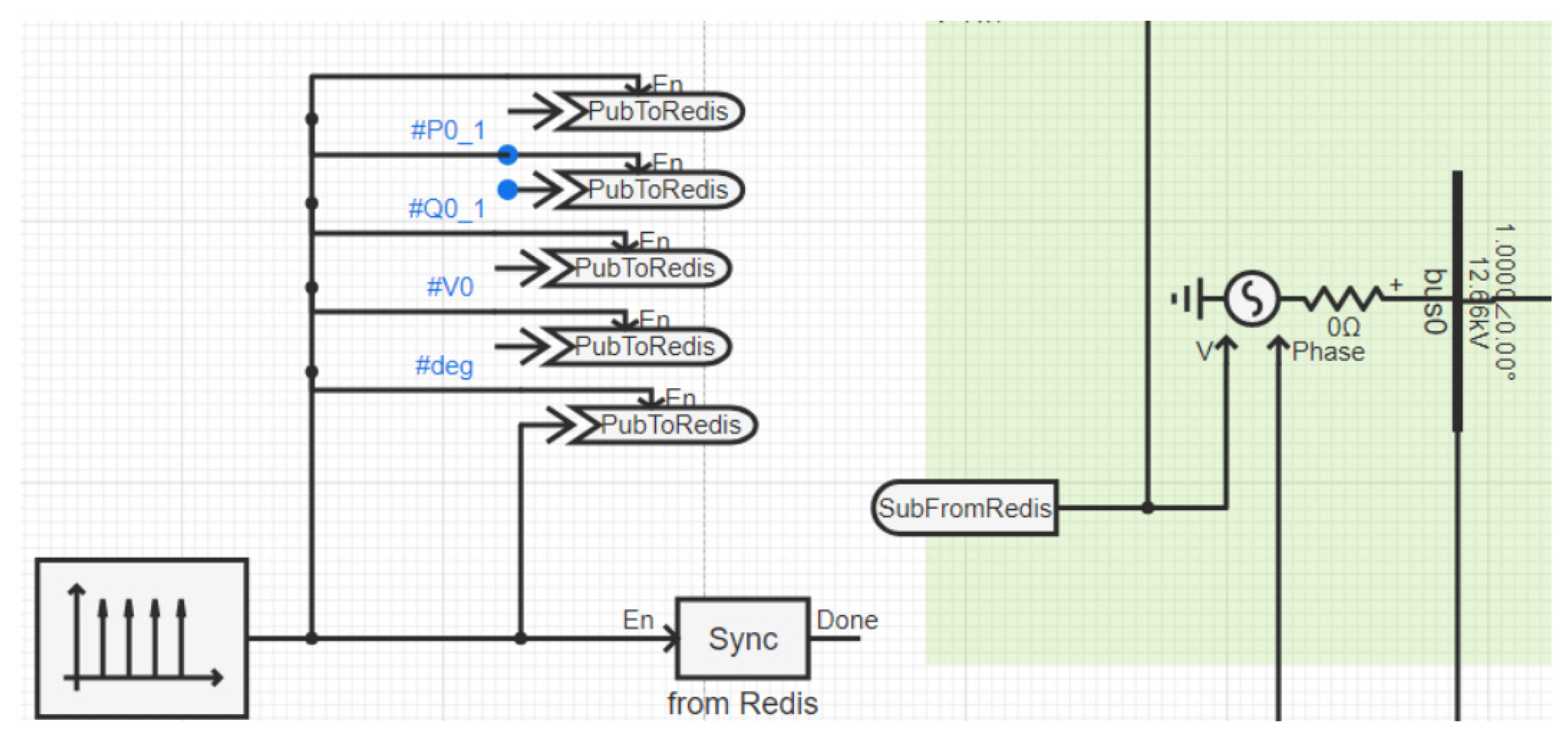
For online closed-loop testing, a co-simulation environment was established. The MPC controller was implemented as a Python script, running separately from the CloudPSS simulation engine. Communication between the Python controller and CloudPSS was facilitated by a Redis (Remote Dictionary Server) instance acting as a message broker. Specific CloudPSS components (Sync, PubToRedis, SubFromRedis) were configured to manage the simulation time steps and data exchange. The Sync component pauses the simulation at predefined intervals ( Δ t ) and resumes it upon receiving a signal via Redis. The PubToRedis components publish measurements (P, Q, V, δ ) from the CloudPSS model to specific Redis channels. A SubFromRedis component subscribes to a Redis channel to receive the voltage setpoint computed by the Python controller, which is then fed to a controlled voltage source at the PCC in the CloudPSS model. This setup allows for pseudo-real-time interaction, testing the controller’s performance within a closed loop involving the detailed DN simulation. Figure 3 illustrates this interface.

4.2. The Benchmark Distribution Network

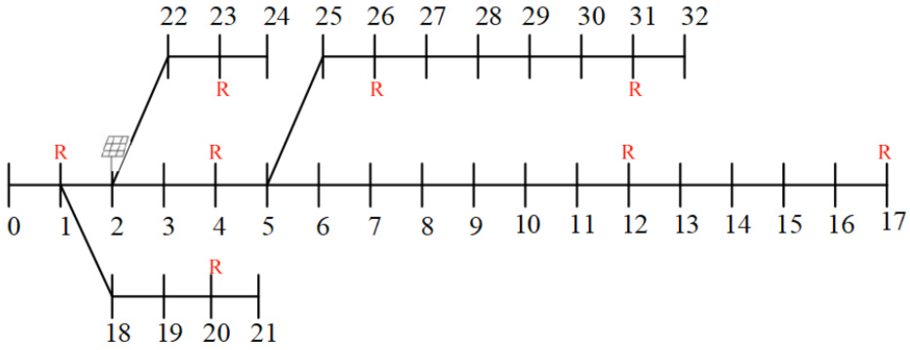
The test system used in this study is a modified version of the standard IEEE 33-bus distribution network. The base topology is shown in Figure 4. To represent a modern DN with complex load dynamics, the following modifications were made:
  • A PV microgrid with a capacity of 0.178 MVA was connected to Node 2.
  • Static constant-impedance loads (R = 500 Ω ) were added at Nodes 1, 4, 12, 17, 20, 23, 26, and 31, in addition to the original constant-power loads.
  • The network is supplied from Node 0 through a step-down transformer (at a 1.2:1 ratio from primary to secondary) connected to a controllable voltage source representing the PCC at the secondary side. The nominal secondary voltage is 12.66 kV line to line.
Detailed load and line parameters were set based on the standard IEEE 33-bus system with minor adjustments. The base power for the per unit calculations was 6.34 MW.

4.3. Data Generation and Training Scenarios

Time-series data for training the NODE model was generated using CloudPSS simulations of the benchmark DN. To ensure the model learned the dynamic response under various conditions, voltage perturbations were applied at the PCC using a controlled voltage source. For the NODE model, the inputs (V, δ ) and outputs (P, Q) were used as nominal values without normalization. V is in kV, δ is in radians, P is in MW, and Q is in MVar. The data generation focused on two scenarios:
  • A single disturbance: The voltage undergoes a step change at a specific time during the simulation. Multiple simulations were run with varying initial voltages and step change magnitudes (an initial voltage randomized between 0.95 V n o m and 1.05 V n o m , a step change to 90 % to 110 % of the initial value). Data segments of a 1 s length around the step change were collected. This yielded 995 data segments for training/testing.
  • A continuous disturbance: The voltage is continuously varied by combining low-frequency large perturbations (random values between 1.2 kV and 1.2 kV, updated at 0.1 Hz) and high-frequency small fluctuations (random values between 0.08 kV and 0.08 kV, filtered and updated at 10 Hz) fed into the controlled voltage source. Longer simulations (53 s each) were run, and the data ( V ( t ) , δ ( t ) , P ( t ) , Q ( t ) at the PCC) was segmented into 2.5 s intervals. A total of 50 such simulations were run with the base voltage randomized between 0.95 V n o m and 1.05 V n o m , yielding 1000 segments of 2.5 s data.
The dataset generated under a continuous disturbance was used for the final model training and validation. This scenario was chosen because a spectrally rich input signal (combining low- and high-frequency perturbations) excites a wider range of system dynamics compared to simple step changes. Training on these more diverse trajectories helps the model learn a more general representation of the network’s behavior and reduces the risk of overfitting to specific transient events. The data was split into training and testing sets (800 segments for training and 200 for testing). Thus, the final training dataset corresponded to a total simulation duration of 800 segments × 2.5 s/segment = 2000 s.

4.4. The MPC Test Scenarios and Metrics

The performance of the linearized NODE-MPC controller was evaluated through both offline and online tests. The control interval Δ t was set to 0.1 s for the online tests, and the prediction/control horizon N p = N c was set to 9 steps.

4.4.1. Offline Tests (Using the Trained NODE Model as a Plant)

These tests assessed the fundamental capabilities of the controller using the trained NODE model as a substitute for the actual DN:
  • Reference tracking: Step changes and varying reference signals P r e f ;
  • Constraint handling: Scenarios where the control action hits the V m i n (0.9 pu) or V m a x (1.1 pu) limits;
  • Parameter sensitivity: The impact of varying the weights α , β and control interval Δ t .

4.4.2. Online Co-Simulation Tests (Using CloudPSS as the Plant)

These tests assessed the controller’s performance in a closed loop with the detailed CloudPSS simulator using the co-simulation setup described in Section 4:
  • Basic tracking: Step changes in P r e f ;
  • Complex tracking: Following more dynamic P r e f trajectories;
  • CVR scenario: Applying a stepped reduction profile to P r e f (e.g., from 100% to 98%, then 96% of the nominal power) to simulate a CVR objective;
  • Supply–demand balancing: Tracking a fluctuating P r e f profile potentially representing available renewable generation.
The nominal power P r a t e d was 6.34 MW.

4.4.3. Performance Metrics

The following metrics were used for evaluation:
  • The NODE model’s accuracy: the mean squared error (MSE), Mean Absolute Error (MAE), and Relative Error (RE) between the NODE model’s predicted power ( P ^ , Q ^ ) and the simulated power from CloudPSS.
  • The MPC controller’s performance: The Root Mean Squared Error (RMSE) between the actual DN power P ( t ) and the reference P r e f ( t ) , the adherence to the voltage constraints ( V m i n V V m a x ), and the computational time required to solve the QP problem at each control step.

5. Results and Discussion

5.1. NODE Model Validation

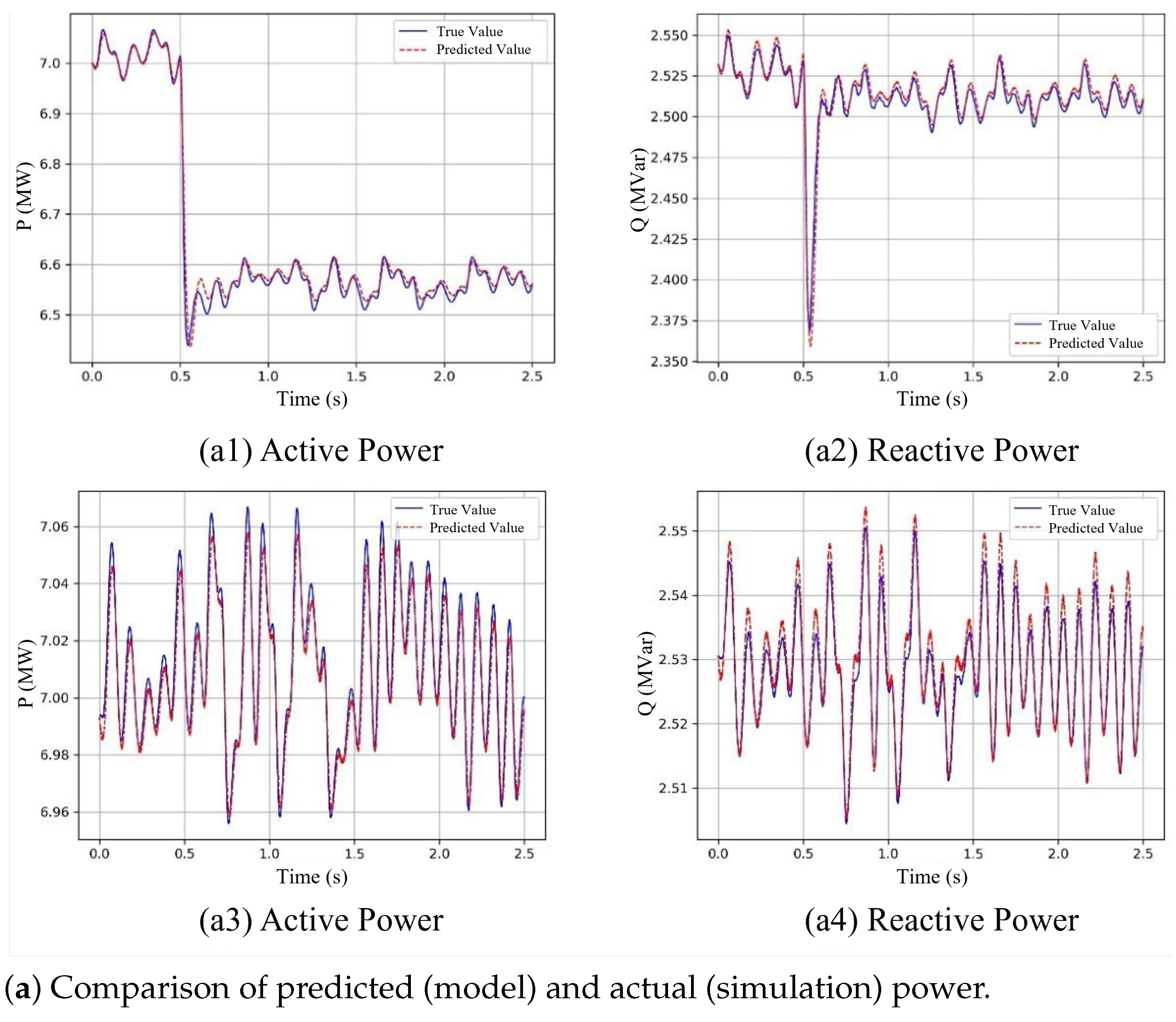
The NODE model was trained using data generated from the continuous disturbance scenario. For the neural network f θ within the NODE, we empirically tested various architectures, including two, three, and four hidden layers with 128, 256, and 512 neurons per layer, respectively. We found that a configuration with three hidden layers, each containing 512 neurons, provided the optimal balance between modeling accuracy and computational efficiency for the complex distribution network dynamics. The training process used the Adam optimizer with an initial learning rate of 0.007, a batch size of 32, and a learning rate decay schedule where the rate was multiplied by 0.7 every 60 epochs. The loss function was the mean squared error (MSE). Training was run for 600 epochs. Figure 5 shows the comparison between the power predicted by the trained NODE model and the ground truth data from the CloudPSS simulation for a sample test trajectory. The model accurately captures both the steady-state power levels and the transient dynamics following voltage fluctuations.
Th quantitative accuracy metrics for the test dataset under continuous disturbances are summarized in Table 1.
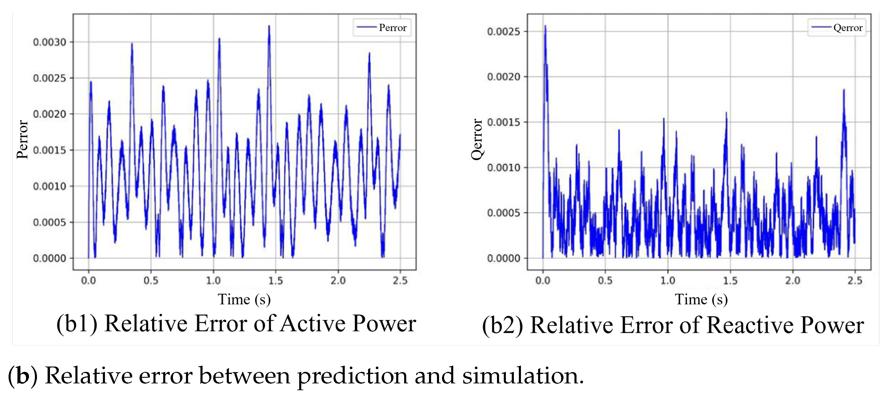
The quantitative accuracy metrics for the test dataset under continuous disturbances are summarized in Table 1. The maximum relative errors observed were below 0.35% for active power and 0.3% for reactive power, indicating a high degree of accuracy. The normalized MSE for both active and reactive power is in the order of 10 3 , further underscoring the model’s precision. The model effectively learned the complex aggregate dynamics from the PCC measurements alone, without needing details on the internal network. The ability to accurately capture these dynamics from terminal measurements is a key advantage for modeling complex or partially unknown networks. A key consideration for any data-driven model is its ability to generalize. The proposed NODE model will maintain its accuracy as long as the underlying network dynamics remain relatively stable. However, a significant structural change, such as a major line outage or the connection of a large new industrial load, would alter the system’s aggregate response and invalidate the current model. This limitation highlights the necessity of a monitoring and retraining strategy for practical deployment. As shown in the validation, the model can be retrained efficiently (e.g., fine-tuning in under an hour on a standard GPU). This capability is crucial, as it allows the dynamic equivalent to be periodically updated to adapt to long-term changes in the network topology or load composition, ensuring its continued accuracy.

5.2. MPC Performance—Offline Analysis

Offline tests using the trained NODE model as the plant confirmed the functionality of the linearized MPC controller. Key findings include
  • Reference tracking: The controller effectively steered the system power towards the desired reference P r e f .
  • Constraint handling: When P r e f demanded voltages beyond the limits ( V m i n / V m a x ), the controller saturated the voltage at the boundary, respecting the constraints.
  • Parameter tuning: Adjusting the weights α and β allowed the tracking accuracy to be traded off against the voltage deviation. Prioritizing tracking ( α > β ) led to a faster power response, while prioritizing voltage stability ( β > α ) resulted in smoother voltage profiles but potentially slower or less exact tracking.
  • Control intervals: Reducing the control interval Δ t generally led to a faster response but could introduce undesirable voltage spikes or instability if too small. A value of Δ t = 0.1 s provided a good balance between responsiveness and smooth control action.
  • Computational efficiency: The linearization successfully converted the complex optimization into a QP problem. The QP solve time using CVXOPT was typically less than 0.1 s on the standard computing hardware for a prediction horizon of 9 steps, well within the typical control interval of 0.1 s, confirming the feasibility for real-time implementation.
These results validated the core design of the linearized NODE-MPC before testing it with the more complex CloudPSS simulator.

5.3. MPC Performance—Online Co-Simulation Validation

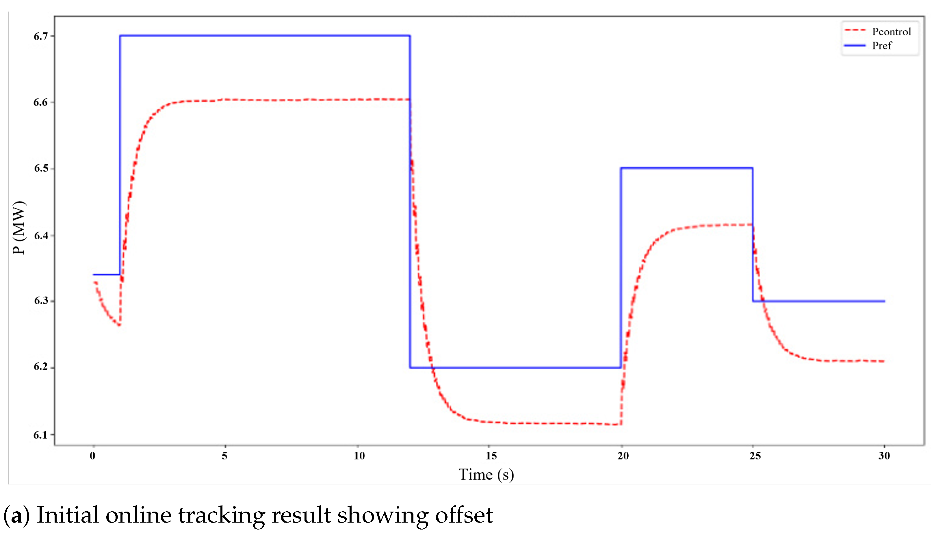
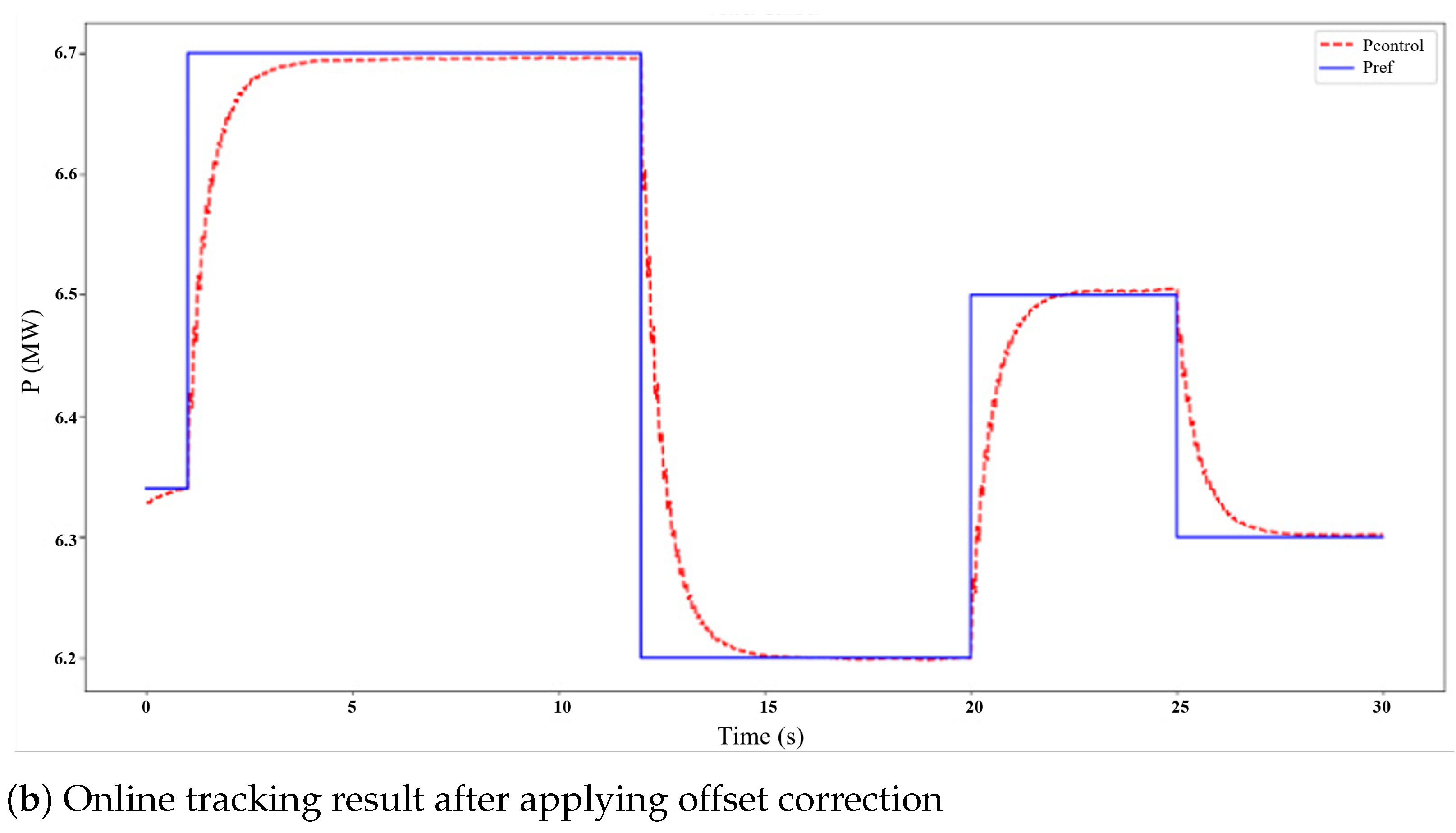
The online co-simulation tests provided a more realistic assessment, revealing a slight systematic offset between the power achieved in the CloudPSS simulation and the reference P r e f targeted by the controller (Figure 6a). This offset (approximately 0.09 MW) is attributed to minor discrepancies between the simplified dynamics captured by the linearized NODE model and the high-fidelity simulation, potentially due to model mismatches or approximations made during linearization.
A straightforward corrective measure was implemented to address this steady-state error. By observing the average offset during the initial tests, a constant correction term (0.09 MW) was added to the reference P r e f within the controller’s QP formulation. As shown in Figure 6b, this simple calibration effectively eliminated the steady-state tracking error for the tested scenarios, bringing the simulated power very close to the desired target (a steady-state error of less than 0.005 MW). While effective here, this highlights the practical challenge of model–plant mismatches. More advanced methods for handling this are discussed in Section 5.5.
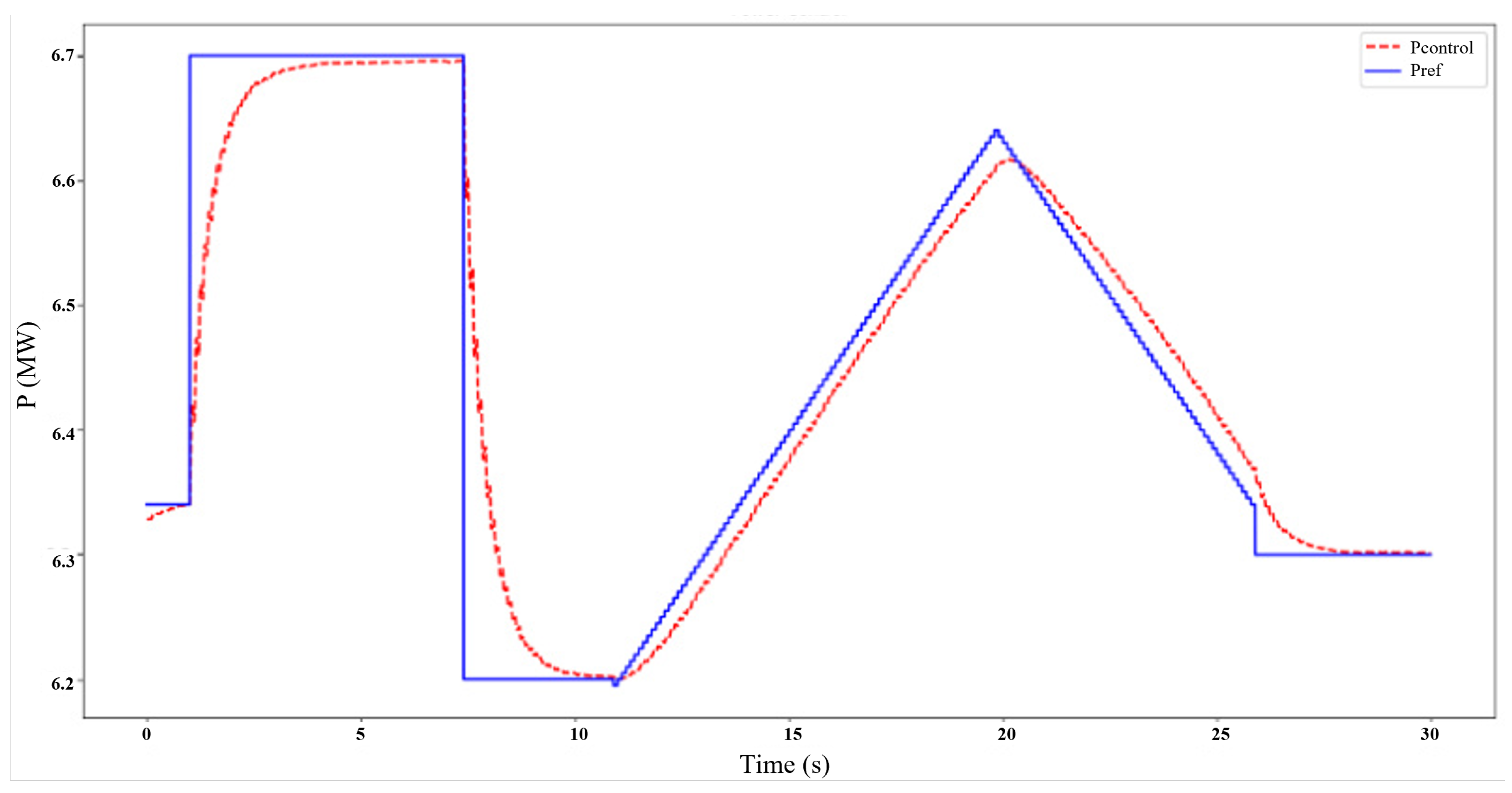
With the correction applied, the controller demonstrated an excellent tracking performance even for complex, time-varying reference signals, as illustrated in Figure 7.
The quantitative performance metrics from the online co-simulation tests are summarized in Table 2.
The RMSE for complex trajectory tracking with correction was visually very low due to the close alignment, consistent with the sub-0.005 MW steady-state error. The error bars/confidence intervals are not usually reported for these types of time series trajectory tracking comparisons in control applications; instead, the performance is typically shown through plots and key error metrics like the steady-state error or RMSE over specific periods.

5.4. Application Scenario Demonstrations

Two application scenarios were simulated to showcase the practical utility of the controller.

5.4.1. Conservation Voltage Reduction (CVR)

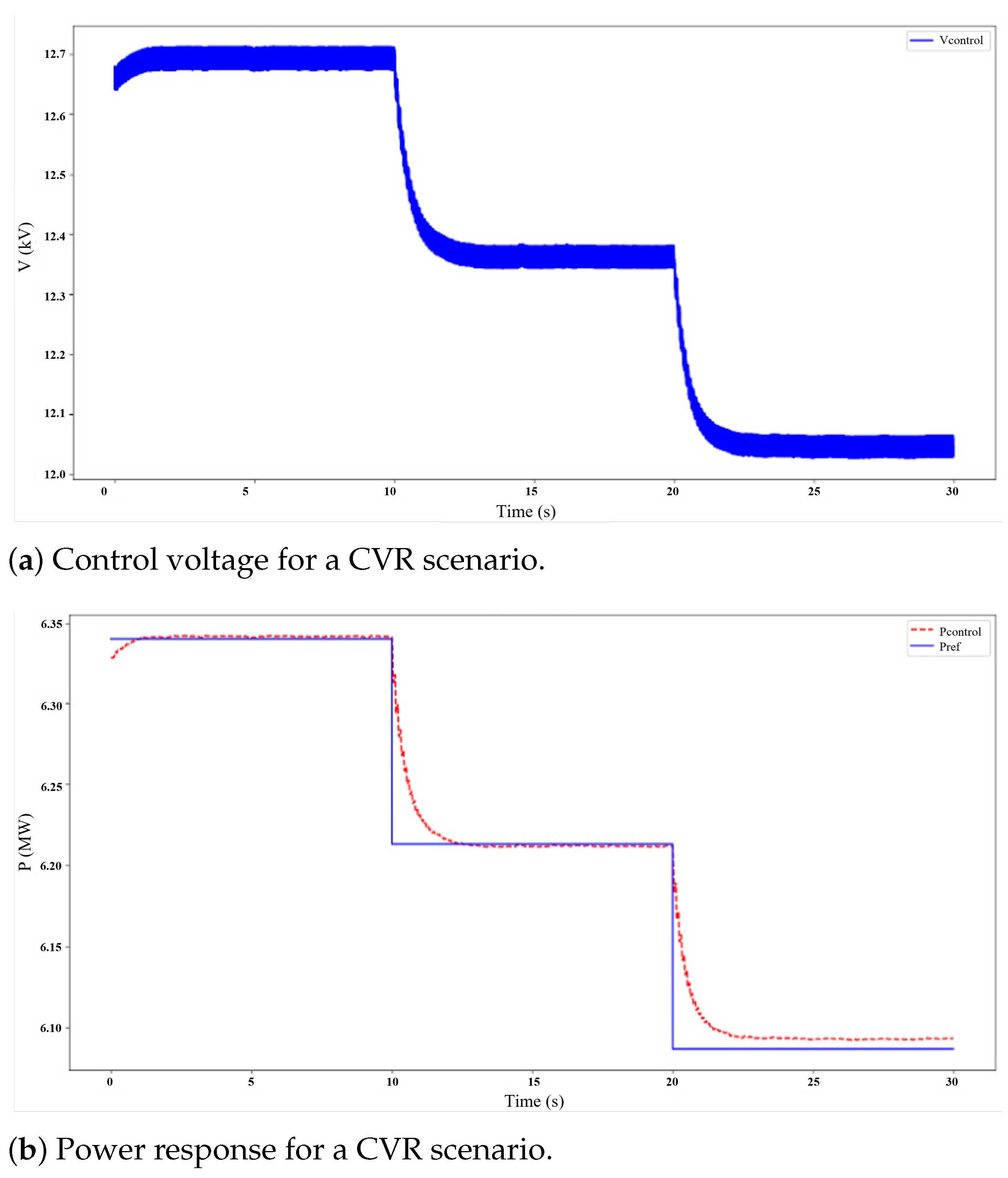
The controller was tasked with reducing the DN’s power consumption in steps (e.g., to 98% and then 96% of the nominal power, relative to the nominal power of 6.34 MW) by lowering the PCC’s voltage. Figure 8 shows the results with α = 1 , β = 0 , prioritizing the tracking accuracy. The controller smoothly adjusted the voltage (Figure 8a) to achieve the target power levels accurately (Figure 8b). It is also demonstrated that increasing β allows the amount of power reduction to be traded off against the magnitude of the deviation in the voltage, providing flexibility for operators in balancing the energy saving with keeping the voltage quality closer to nominal.

5.4.2. Supply–Demand Balancing

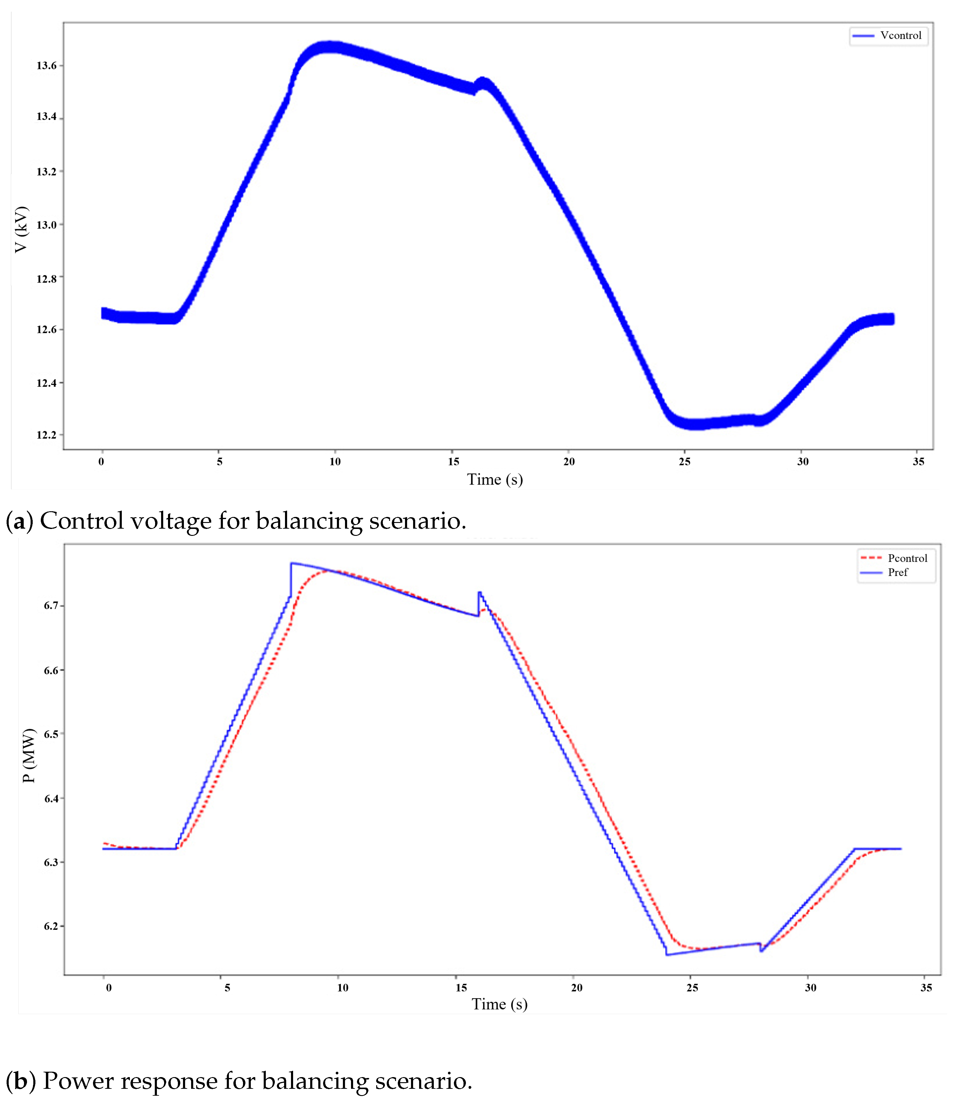
To simulate balancing the DN load with fluctuating local renewable generation, the controller’s reference P r e f was set to a time-varying profile potentially representing the available generation. Figure 9 shows that the controller successfully modulated the DN’s power consumption (Figure 9b) to track this fluctuating target by adjusting the PCC’s voltage (Figure 9a). This demonstrates the potential to use voltage control via MPC to enhance the flexibility of DNs and support the grid’s stability, especially with increasing variable generation.

5.5. Discussion

The results collectively demonstrate the effectiveness of the proposed NODE modeling and the linearized MPC control framework. However, this study also highlights key challenges. The systematic offset observed in the online tests underscores the practical issue of model–plant mismatches. While a simple static correction was effective here, a more robust solution is desirable. The NODE model accurately captured the complex aggregate dynamics of the modified distribution network from the PCC measurements, showing high accuracy metrics (Table 1). This data-driven approach reduces the reliance on detailed internal component parameters, offering an advantage for modeling heterogeneous networks where such details might be unavailable or change over time. The NODE’s continuous-time formulation is physically intuitive for dynamic systems compared to discrete-time models.
The local linearization technique successfully enabled the integration of this sophisticated non-linear model into an MPC framework that was computationally efficient enough for real-time control. The observed QP solve times of less than 0.1 s within a 0.1 s control interval for a nine-step horizon validate its practical feasibility, demonstrating that the controller can compute the optimal action before the next control instant. However, this also indicates a relatively limited computational margin. For real-world implementation, an additional computational overhead must be considered, including the data acquisition, pre-processing, linearization calculations, and communication latency. While our results show its feasibility on standard computing hardware, deploying this framework in a live system would benefit from optimized QP solver libraries or dedicated hardware (e.g., FPGAs, DSPs) designed for real-time control, which could achieve solve times within the millisecond range for problems of this size. Furthermore, significant communication delays between the controller and actuators could reduce the effective computational window. In such scenarios, advanced strategies like explicit delay modeling within the MPC formulation or event-triggered control could be explored to maintain the performance and robustness.
The online co-simulation with a high-fidelity simulator confirmed the controller’s ability to regulate power in a closed loop, achieving a good tracking performance (low steady-state error after correction; see Table 2) while respecting the voltage constraints. The observed systematic offset in the initial online tests highlights the practical challenge of model mismatches between the learned dynamics and the true system (high-fidelity simulator), even with a highly accurate model. The simple offset correction applied effectively mitigated this in the tested scenarios, suggesting the need for adaptation or calibration mechanisms in real-world deployments. The application scenarios further highlighted the practical relevance for CVR and grid balancing services, demonstrating how voltage control can be used to achieve these objectives dynamically.
The observed QP solve times of less than 0.1 s within a 0.1 s control interval for a nine-step horizon validate its practical feasibility.
Limitations of the current study include the reliance on simulation data for training. Real-world data would introduce critical challenges such as communication latency, measurement loss, sensor errors, and voltage control device limits, which could significantly impact the model’s accuracy and the controller’s performance. Developing mechanisms to robustly handle these factors is crucial for practical deployments. The observed offset in the co-simulation suggests potential model mismatches, which might require more sophisticated adaptation mechanisms than simple offset correction in practice.
The linearization introduces approximation errors, although the receding-horizon nature of MPC helps to mitigate this by re-linearizing at each step. While a simple static correction was effective here, a more robust solution is desirable. More advanced methods incorporating stronger non-linearities, such as second-order approximations or piecewise linear models, could enhance the accuracy further at the cost of potentially increased computational complexity. The current formulation primarily focuses on the P-V relationship for active power control, neglecting potential stronger coupling with reactive power (Q). It also treats the voltage angle ( δ ) as a measured disturbance rather than a controlled or predicted variable. While this is an effective simplification for the targeted applications, a more comprehensive multi-input, multi-output (MIMO) control strategy could be explored in the future. Scalability to much larger and more complex networks also warrants further investigation, both in terms of the model training data requirements and the computational burden for linearization/QP solve times. While this work demonstrates feasibility for the tested network, the performance might differ for larger systems.
Despite these limitations, the proposed framework offers a promising data-driven approach that leverages the strengths of continuous-time deep learning for modeling and efficient QP solvers for control, providing a valuable tool for advanced power regulation in modern distribution networks.
Equally, for practical implementation, periodic retraining of the NODE model is essential to maintain its accuracy as the distribution network evolves. The trigger for such retraining could be based on several criteria. A primary trigger would be performance degradation, where the real-time prediction error of the model consistently exceeds a predefined threshold. For example, if the Mean Absolute Error (MAE) between the predicted and measured power surpasses a set percentage over a 24 h window, an automated retraining process could be initiated using newly collected data. A second category of triggers would be event-driven. Acknowledged changes in the network topology, such as the commissioning of a new substation, a major line reconfiguration, or the integration of a large-scale renewable plant, would necessitate a mandatory model update to capture the new system dynamics.

6. Conclusions

This paper addressed the challenge of modeling and controlling modern complex distribution networks by proposing a novel framework combining Neural Ordinary Differential Equations (NODEs) for data-driven dynamic modeling and Model Predictive Control (MPC) for active power regulation. The proposed controller successfully regulated the active power of a high-fidelity simulated distribution network with a steady-state tracking error of less than 0.005 MW. This performance was achieved by solving the underlying optimization problem in under 0.1 s per control step, confirming the framework’s potential for real-time application.
The key contributions include (1) demonstrating the capability of NODEs to accurately model the aggregate dynamic power response of a DN using only PCC measurements, effectively capturing the continuous-time behavior; (2) developing a computationally efficient MPC strategy by employing local linearization of the trained NODE model, enabling the formulation of the control problem as a standard Quadratic Programming (QP) problem; (3) validating the entire framework through extensive simulations, including an offline analysis and online co-simulation with a detailed DN simulator (CloudPSS), confirming the model’s accuracy, control effectiveness, and computational feasibility (typical QP solve times <0.1 s); and (4) illustrating the practical applicability through scenarios like Conservation Voltage Reduction (CVR) and supply–demand balancing.
The proposed framework offers a significant advancement by providing an end-to-end data-driven approach to advanced DN control. It leverages the modeling power of continuous-time deep learning (NODEs) while ensuring real-time applicability through efficient linearization and QP-based MPC. This could potentially enhance the grid’s operation, improve the energy efficiency, and facilitate the integration of renewable energy resources.
Future research directions include
  • Extending the control objectives from aggregating the power regulation and voltage constraint adherence based on PCC measurements to multi-objective optimization to include economic costs, internal loss reductions, and explicit renewable energy dispatching, which would necessitate greater internal network observability or advanced state estimation techniques.
  • Developing adaptive mechanisms to handle model mismatches and time-varying network conditions, such as online NODE parameter updates or adaptive linearization schemes. Exploring the use of higher-order approximations or piecewise linear models within the MPC framework could enhance the control accuracy for highly dynamic or widely varying operating conditions, while carefully managing the computational efficiency.
  • Investigating the inclusion of the reactive power and voltage angle control within the MPC framework could broaden its applicability.
  • Exploring extending the NODE model to Neural Stochastic Differential Equations (Neural SDEs) to explicitly quantify the forecast uncertainty to enhance the framework’s robustness against inherent system stochasticity and measurement noise. This would enable the development of robust or stochastic MPC strategies that could maintain reliable control under uncertain conditions.
  • Assessing the scalability and robustness of the approach for significantly larger, more complex distribution systems. Further quantitative comparisons with other state-of-the-art data-driven modeling and control techniques would provide valuable context.
  • Testing and validating the framework in real-world scenarios, explicitly addressing the implications of the communication latency, measurement loss, sensor errors, and voltage control devices’ limits. This would involve investigating robust state estimation techniques and delay compensation strategies within the MPC framework.

Author Contributions

Conceptualization, L.W. and T.X.; Methodology, L.W., H.H., L.X. and G.L.; Software, J.X.; Validation, J.X., H.H. and G.L.; Formal analysis, J.X.; Investigation, L.X.; Resources, L.W.; Data curation, H.H.; Writing—original draft, L.W.; Writing—review & editing, J.X., H.H., L.X., G.L. and T.X.; Visualization, L.X.; Supervision, T.X.; Funding acquisition, L.W. and T.X. All authors have read and agreed to the published version of the manuscript.

Funding

This paper was supported by the Science and Technology Project of China Southern Power Grid Co., Ltd. (Project No.: GXKJXM20222192).

Data Availability Statement

The data presented in this study are available on request from the corresponding author. Data availability is restricted by the policies of the funding agency for this research.

Conflicts of Interest

Authors Libin Wen, Jinji Xi, Hong Hu, Li Xiong and Guangling Lu were employed by the Electric Power Research Institute of Guangxi Power Grid Co., Ltd. The remaining author declares that the research was conducted in the absence of any commercial or financial relationships that could be construed as a potential conflict of interest.

Nomenclature

tA continuous-time variable
kA discrete-time index for control steps
Δ t A discretization time step for the MPC control interval
P ( t ) , P k The active power consumed by the DN at the PCC (continuous, discrete) [MW]
Q ( t ) , Q k The reactive power consumed by the DN at the PCC (continuous, discrete) [MVar]
V ( t ) , V k The voltage magnitude (RMS, line to line) at the PCC (continuous, discrete) [kV]
δ ( t ) , δ k The voltage angle at the PCC (continuous, discrete) [rad or deg]
x ( t ) , x k The state vector of the DN model, x ( t ) = [ P ( t ) , Q ( t ) ] T
z ( t ) , z k The input vector to the DN model, z ( t ) = [ V ( t ) , δ ( t ) ] T
f θ A neural network function parameterizing the ODE, with the parameters θ
x ^ ( t ) , x ^ k | k 1 The state vector predicted by the model (continuous, discrete)
P ^ k + j + 1 | k The predicted active power at step k + j + 1 , based on the info at step k
D The training dataset
L ( θ ) The loss function for model training
u k The control input at discrete time k, u k = V k
V k + j | k The planned voltage at step k + j decided at step k
N p The prediction horizon (number of steps)
N c The control horizon (number of steps) (in this work, N c = N p )
V k The sequence of control inputs at step k, V k = [ V k | k , , V k + N p 1 | k ] T
P r e f , k The reference active power target at time step k
P r e f The vector of reference active power targets over the prediction horizon
J ( V k ) The MPC cost function at time step k
α , β Weighting factors in the cost function
V n o m The nominal voltage magnitude [kV]
V m i n , V m a x The minimum and maximum allowable voltage magnitudes [kV]
NODENeural Ordinary Differential Equation
MPCModel Predictive Control
DNDistribution network
PCCPoint of common coupling
DERDistributed energy resource
PVPhotovoltaic
CVRConservation Voltage Reduction
QPQuadratic Programming
MLPMulti-Layer Perceptron
MSEMean squared error
MAEMean Absolute Error
RMSERoot Mean Squared Error
RERelative error
ADAutomatic Differentiation
ANNArtificial Neural Network
RNNRecurrent Neural Network
LSTMLong Short-Term Memory
ZIPConstant-impedance, constant-current, constant-power model
IMInduction motor

References

  1. National Energy Administration. Notice on Issuing the Measures for the Supervision of Fair and Open Grid Access. 2021. Available online: https://www.gov.cn/gongbao/content/2022/content_5667313.htm (accessed on 3 December 2024).
  2. National Energy Administration. Transcript of the Press Conference for the First Quarter of 2023. 2023. Available online: http://www.nea.gov.cn/2023-02/13/c_1310697149.htm (accessed on 5 December 2024).
  3. Diaz-Aguiló, M.; Sandraz, J.; Macwan, R.; De Leon, F.; Czarkowski, D.; Comack, C.; Wang, D. Field-validated load model for the analysis of CVR in distribution secondary networks: Energy conservation. IEEE Trans. Power Del. 2013, 28, 2428–2436. [Google Scholar] [CrossRef]
  4. Zhang, Q.; Dehghanpour, K.; Wang, Z. Distributed CVR in unbalanced distribution systems with PV penetration. IEEE Trans. Smart Grid 2019, 10, 5308–5319. [Google Scholar] [CrossRef]
  5. Arif, A.; Wang, Z.; Wang, J.; Chen, C. Load modeling—A review. IEEE Trans. Smart Grid 2018, 9, 5986–5999. [Google Scholar] [CrossRef]
  6. Bokhari, A.; Alkan, A.; Dogan, R.; Diaz-Aguiló, M.; De Leon, F.; Czarkowski, D.; Zabar, Z.; Birenbaum, L.; Noel, A.; Uosef, R.E. Experimental determination of the ZIP coefficients for modern residential, commercial, and industrial loads. IEEE Trans. Power Del. 2014, 29, 1372–1381. [Google Scholar] [CrossRef]
  7. Samadi, A.; Soder, L.; Shayesteh, E.; Hooshmand, R.A. Static equivalent of distribution grids with high penetration of PV systems. IEEE Trans. Smart Grid 2015, 6, 1763–1774. [Google Scholar] [CrossRef]
  8. Zali, S.M.; Milanović, J.V. Generic model of active distribution network for large power system stability studies. IEEE Trans. Power Syst. 2013, 28, 3126–3133. [Google Scholar] [CrossRef]
  9. Choi, B.-K.; Li, D.C.H.; Li, Y. Development of composite load models of power systems using on-line measurement data. J. Electr. Eng. Technol. 2006, 1, 161–169. [Google Scholar] [CrossRef]
  10. Milanović, J.V.; Zali, S.M. Validation of equivalent dynamic model of active distribution network cell. IEEE Trans. Power Syst. 2013, 28, 2101–2110. [Google Scholar] [CrossRef]
  11. Ma, R.; Ma, J.; Hill, D.J. Composite load modeling via measurement approach. IEEE Trans. Power Syst. 2006, 21, 663–672. [Google Scholar]
  12. Ma, J.; Ma, R.; Hill, D.J. Load modeling by finding support vectors of load data from field measurements. IEEE Trans. Power Syst. 2006, 21, 726–735. [Google Scholar]
  13. Wang, X.; Wang, Y.; Shi, D.; Wang, J.; Wang, Z. Two-stage WECC composite load modeling: A double deep Q-learning networks approach. IEEE Trans. Smart Grid 2020, 11, 4331–4344. [Google Scholar] [CrossRef]
  14. Cai, C.; Liu, H.; Tao, Y.; Zhang, J.; Song, W. Microgrid equivalent modeling based on long short-term memory neural network. IEEE Access 2020, 8, 23120–23133. [Google Scholar] [CrossRef]
  15. Ji, Y.; Buechler, E.; Rajagopal, R. Data-driven load modeling and forecasting of residential appliances. IEEE Trans. Smart Grid 2020, 11, 2652–2661. [Google Scholar] [CrossRef]
  16. Abdelaziz, A.Y.; Badr, M.A.L.; Younes, A.H. Dynamic load modeling of an Egyptian primary distribution system using neural networks. Int. J. Electr. Power Energy Syst. 2007, 29, 637–649. [Google Scholar] [CrossRef]
  17. Azmy, A.M.; Erlich, I.; Sowa, P. Artificial neural network-based dynamic equivalents for distribution systems containing active sources. IEE Proc.-Gener. Transm. Distrib. 2004, 151, 681–688. [Google Scholar] [CrossRef]
  18. Azmy, A.M.; Erlich, I. Identification of dynamic equivalents for distribution power networks using recurrent ANNs. In Proceedings of the IEEE PES Power Systems Conference and Exposition, New York, NY, USA, 10–13 October 2004; pp. 348–353. [Google Scholar]
  19. Denecke, J.; Erlich, I. Dynamic equivalents of active distribution networks. In Proceedings of the 2017 IEEE Power & Energy Society General Meeting, Chicago, IL, USA, 16–20 July 2017; pp. 1–5. [Google Scholar]
  20. Stankovic, A.M.; Saric, A.T.; Milosevic, M. Identification of nonparametric dynamic power system equivalents with artificial neural networks. IEEE Trans. Power Syst. 2003, 18, 1478–1486. [Google Scholar] [CrossRef]
  21. Saviozzi, M.; Massucco, S.; Silvestro, F. Implementation of advanced functionalities for Distribution Management Systems: Load forecasting and modeling through Artificial Neural Networks ensembles. Electr. Power Syst. Res. 2019, 167, 230–239. [Google Scholar] [CrossRef]
  22. He, R.-M.; Germond, A.J. Comparison of dynamic load modeling using neural network and traditional method. In Proceedings of the Second International Forum on Applications of Neural Networks to Power Systems, Kobe, Japan, 19–22 April 1993; pp. 253–258. [Google Scholar]
  23. Visconti, I.F.; Lima, D.A.; Costa, J.M.C.d.S.; Sobrinho, N.R.d.B.C. Measurement-based load modeling using transfer functions for dynamic simulations. IEEE Trans. Power Syst. 2014, 29, 111–120. [Google Scholar] [CrossRef]
  24. Ospina, L.D.P.; Salazar, V.U.; Ospina, D.P. Dynamic equivalents of nonlinear active distribution networks based on Hammerstein-Wiener models: An application for long-term power system phenomena. IEEE Trans. Power Syst. 2022, 37, 3799–3809. [Google Scholar] [CrossRef]
  25. Chen, R.T.Q.; Rubanova, Y.; Bettencourt, J.; Duvenaud, D.K. Neural ordinary differential equations. In Proceedings of the Advances in Neural Information Processing Systems 31: Annual Conference on Neural Information Processing Systems 2018, NeurIPS 2018, Montréal, QC, Canada, 3–8 December 2018; Volume 31. [Google Scholar]
  26. Kidger, P. On neural differential equations. arXiv 2022, arXiv:2202.02435. [Google Scholar]
  27. Lee, K.; Parish, E.J. Parameterized neural ordinary differential equations: Applications to computational physics problems. Proc. R. Soc. A 2021, 477, 20210162. [Google Scholar] [CrossRef]
  28. Lei, D.; Wu, K.; Zhang, L.; Li, W.; Liu, Q. Neural ordinary differential grey model and its applications. Expert Syst. Appl. 2021, 177, 114923. [Google Scholar] [CrossRef]
  29. Xiao, T.; Chen, Y.; Huang, S.; Zhang, R.; Wang, Z.; Sun, Y. Feasibility study of neural ODE and DAE modules for power system dynamic component modeling. IEEE Trans. Power Syst. 2023, 38, 1267–1279. [Google Scholar] [CrossRef]
  30. Preiss, R.F.; Warnock, V.J. Impact of voltage reduction on energy and demand. IEEE Trans. Power App. Syst. 1978, PAS-97, 1665–1671. [Google Scholar] [CrossRef]
  31. Scalley, B.R.; Kasten, D.G. The effects of distribution voltage reduction on power and energy consumption. IEEE Trans. Educ. 1981, 24, 210–216. [Google Scholar] [CrossRef]
  32. Wang, Z.; Wang, J. Review on implementation and assessment of conservation voltage reduction. IEEE Trans. Power Syst. 2014, 29, 1306–1315. [Google Scholar] [CrossRef]
  33. Singh, R.; Tuffner, F.; Fuller, J.; Chassin, D.; Kumar, N.P. Effects of distributed energy resources on conservation voltage reduction (CVR). In Proceedings of the 2011 IEEE Power and Energy Society General Meeting, Detroit, MI, USA, 24–28 July 2011; pp. 1–7. [Google Scholar]
  34. Efheij, H.; Albagul, A.; Ammar Albraiki, N. Comparison of Model Predictive Control and PID Controller in Real Time Process Control System. In Proceedings of the 19th International Conference on Sciences and Techniques of Automatic Control and Computer Engineering (STA), Sousse, Tunisia, 24–26 March 2019; pp. 64–69. [Google Scholar]
  35. Abdallaoui, S.; Kribèche, A.; Aglzim, E.H. Comparative study of MPC and PID controllers in autonomous vehicle application. In Advances in Automation, Mechanical and Design Engineering; Laribi, M.A., Carbone, G., Jiang, Z., Eds.; Springer: Cham, Switzerland, 2023; Volume 121, pp. 100–110. [Google Scholar]
  36. Akpan, V.A.; Hassapis, G.D. Nonlinear model identification and adaptive model predictive control using neural networks. ISA Trans. 2011, 50, 177–194. [Google Scholar] [CrossRef]
Figure 1. The conceptual structure of the neural ODE (NODE) model for the distribution network dynamics, mapping the current state x ( t ) = [ P , Q ] and input z ( t ) = [ V , δ ] to the state derivative x ˙ ( t ) via the neural network f θ , which is then integrated using an ODE solver to produce the state prediction.
Energies 18 03419 g001
Figure 2. The overall workflow of the proposed framework combining offline NODE training and online linearized NODE-based MPC execution.
Energies 18 03419 g002
Figure 3. A co-simulation interface diagram showing the connection between CloudPSS components (Sync for time synchronization; PubToRedis for measurements of P, Q, V, δ ; SubFromRedis for control voltage) and the external Python MPC controller via Redis channels.
Energies 18 03419 g003
Figure 4. The topology of the modified IEEE 33-bus benchmark distribution network used for the simulation studies.
Energies 18 03419 g004
Figure 5. NODE model validation results under continuous voltage disturbances: (a) comparison of active (P) and reactive (Q) power predicted by the NODE model (red, predicted values) against the simulation data (blue, true values); (b) the relative error for the P and Q predictions.
Energies 18 03419 g005aEnergies 18 03419 g005b
Figure 6. The online co-simulation tracking performance for a step change in P r e f : (a) the initial result showing a steady-state error between the simulated power (red, Pcontrol) and the reference power (blue, Pref). (b) The result after correcting the reference within the MPC, showing a significantly improved tracking accuracy.
Energies 18 03419 g006aEnergies 18 03419 g006b
Figure 7. The online co-simulation tracking performance for a complex reference power trajectory (red: simulated power Pcontrol; blue: reference power Pref).
Energies 18 03419 g007
Figure 8. Demonstration of the CVR application: the MPC controller adjusts the voltage (a) to make the DN’s power consumption ((b), red: simulated power Pcontrol) follow a stepped reduction target ((b), blue: reference power Pref).
Energies 18 03419 g008
Figure 9. Demonstration of the supply–demand balancing application: the MPC controller adjusts the voltage (a) to track the DN’s power consumption ((b), red: simulated power Pcontrol) against a fluctuating reference representing the available generation ((b), blue: reference power Pref).
Energies 18 03419 g009
Table 1. NODE model accuracy metrics (continuous disturbance scenario test set).
MetricActive Power (P)Reactive Power (Q)
Max Relative Error<0.35%<0.30%
Normalized MSE 1.3 × 10 3 1.1 × 10 3
Final Training Loss (MSE) 0.0013
Table 2. MPC performance metrics (online co-simulation with offset correction, Δ t = 0.1 s, N p = 9 ).
MetricValue
Steady-State Error (Corrected)<0.005 MW
Voltage Constraint AdherenceMaintained within [0.9, 1.1] pu
Typical QP Computation Time per Step<0.1 s
Disclaimer/Publisher’s Note: The statements, opinions and data contained in all publications are solely those of the individual author(s) and contributor(s) and not of MDPI and/or the editor(s). MDPI and/or the editor(s) disclaim responsibility for any injury to people or property resulting from any ideas, methods, instructions or products referred to in the content.