Quantitative Assessment Method for Industrial Demand Response Potential Integrating STL Decomposition and Load Step Characteristics

Abstract

With the increasing penetration of renewable energy, power grids face significant challenges in balancing fluctuating renewable generation with flexible demand-side resources. Industrial loads, characterized by substantial consumption and high adjustability, provide critical flexibility to address these challenges; however, existing methods for quantifying their response potential lack sufficient accuracy and comprehensive uncertainty characterization. This study proposes an integrated quantitative assessment framework combining Seasonal-Trend decomposition using Loess (STL), load-step feature extraction, and Gaussian Process Regression (GPR). Historical industrial load data are first decomposed using STL to isolate trend and periodic patterns, while mathematically defined load-step indicators quantify intrinsic adjustability. Concurrently, a multi-dimensional willingness index reflecting past response behaviors and participation records comprehensively characterizes user response capabilities and inclinations. A GPR-based nonlinear mapping between extracted load features and response potential enables precise quantification and robust uncertainty estimation. Case studies verify the effectiveness of the proposed approach, achieving an assessment accuracy of 91.4% and improved confidence interval characterization compared to traditional methods. These findings demonstrate the framework’s significant capability in supporting precise flexibility utilization, thereby enhancing operational stability in power grids with high renewable energy penetration.

1. Introduction

1.1. Motivation and Background

Driven by the global transition towards low-carbon energy structures, the novel power system is undergoing fundamental changes in its coordinated “source–grid–load” operational model. According to the latest statistics from the National Energy Administration [1], China’s installed capacity of renewable energy sources accounted for 42.03% by 2024. This structural shift has introduced dynamic balancing challenges from both the generation and load sides. On the one hand, the inherent volatility and uncertainty of renewable energy sources result in reduced accuracy of generation-side output forecasts [2]; on the other hand, the load side must develop corresponding dynamic response capabilities to ensure system stability. In this context, deeply exploiting flexible load-side resources has emerged as a critical issue for ensuring the secure and economical operation of the novel power system [3].

Demand response (DR) refers to the capability of end-users to adjust their electricity consumption in response to external signals, such as time-based rates or incentive programs. Its effective implementation requires several prerequisites: (i) users must possess adjustable loads with non-critical operational constraints; (ii) communication infrastructure must be capable of issuing real-time or day-ahead instructions; and (iii) there must exist clear economic or regulatory incentives [4]. However, DR faces inherent limitations. These include limited user engagement due to production rigidity, uncertainties in actual response execution, and the lack of standardized assessment tools to evaluate DR potential across heterogeneous user profiles. Additionally, behavioral inertia and misalignment between declared capacity and actual execution further hinder its practical effectiveness [5].

Notably, industrial electricity consumption in China consistently exceeds 66% of total societal electricity consumption [6]. This unique consumption structure offers significant opportunities for load-side flexibility regulation. Compared with commercial and residential loads, industrial users exhibit three notable characteristics: firstly, they consume substantial energy volumes, with single-user regulation potentials reaching megawatt levels; secondly, their production processes inherently allow for interruption and shifting; thirdly, they can achieve minute-to-hour scale power adjustments through optimized production scheduling and equipment start–stop control [7].

1.2. Related Work

As energy-intensive consumers, industrial sectors—particularly heavy industries—are composed of multiple interconnected sub-processes, some of which are highly interdependent and may not tolerate interruptions. This makes industrial demand response (IDR) programs inherently complex [8]. Current IDR potential evaluation approaches primarily focus on constructing user feature datasets to assess their response capabilities, which can be categorized into three main methodologies, as shown in

Table 1. Summary of mainstream industrial DR potential assessment approaches.

Methodology	Description	Advantages	Limitations	References
Comprehensive Evaluation	Multi-index systems using weights and scoring	Intuitive and easy to implement	Requires expert input, low adaptability	[10,11]
Mechanism-based Modeling	Based on physical/operational constraints of equipment	High accuracy for known systems	High data granularity needed, poor generalization	[12,13]
Data-driven Techniques	Regression, clustering, and transfer learning	Adaptive, scalable to large users	Risk of overfitting, depends on data quality	[14,15,16]

: comprehensive evaluation, mechanism-based analysis, and data-driven techniques [9].

Comprehensive evaluation methods establish multi-dimensional index systems to quantify user response potential using relative metrics. For example, ref. [10] introduced the concept of price elasticity from economics to assess users’ demand response potential by combining historical load profiles and time-matched electricity pricing data. However, this approach typically requires fine-grained, device-level data to accurately estimate price elasticity. Similarly, ref. [11] used questionnaire-based surveys to identify key factors influencing user participation; while effective for capturing willingness at a given time, this method is labor-intensive, susceptible to privacy concerns, and lacks timeliness for tracking changes in user potential.

Mechanism-based analyses often rely on decoupled physical modeling under operational constraints. References [12,13] used non-intrusive load-monitoring techniques to gather device-level data and construct physical models. However, these models demand high data resolution and volume for training, and their dependence on device-specific libraries limits generalizability across industrial users, reducing practical applicability.

Data-driven approaches include regression analysis, clustering, and transfer learning. Despite their promise, current studies still face challenges in scenario adaptability and methodological completeness. For instance, ref. [14] proposed a deep subdomain adaptation method that constructs a library of quadratic regression parameters for typical user load patterns and uses neural network-based transfer learning to estimate DR potential. Nevertheless, it overlooks the temporal concentration of actual DR events, which often occur in short 1–2 h windows, resulting in suboptimal feature alignment. Reference [15] employed a Gaussian Process Regression model based on an interruptible vector load framework, but it suffers from two limitations: first, it lacks a precise mathematical definition of load steps, relying instead on heuristic descriptions; second, its applicability is limited to users with clearly stepped load patterns, excluding more volatile industries such as aluminum smelting. In [16], a parameter transfer learning approach was used to assess potential for users with incomplete historical data; while useful during the early stages of DR program rollout, this method assumes holistic parameter transfer and neglects key factors such as sector-specific value-add and usage habits that contribute to response variability among different industrial users.

1.3. Contributions and Organization

Due to user privacy protection requirements [17], conventional monitoring systems can typically access only historical load data. Analysis reveals that the power consumption equipment in industrial settings often operates in a limited set of discrete states [18], resulting in daily load curves that exhibit characteristic “load step” patterns. Experimental findings in [19] indicate a strong correlation between the magnitude and temporal distribution of load steps and a user’s adjustable demand response potential. Motivated by these physical characteristics and empirical relationships, this study proposes a novel assessment framework that integrates load decomposition with load step extraction to evaluate the demand response potential of industrial users.

This study proposes a novel, hybrid industrial demand response assessment framework that combines STL decomposition, mathematically defined load step characterization, and multi-dimensional response willingness quantification. The scientific novelty lies in three key aspects: (i) introducing a physically interpretable load step matrix as a generalized indicator of flexibility; (ii) fusing behavioral and structural features into a unified Gaussian Process Regression (GPR) model to enhance uncertainty modeling; and (iii) achieving probabilistic estimation of DR potential with confidence bounds, which has rarely been done in prior work.

The remainder of this paper is organized as follows: Section 2 presents the proposed methodology for extracting load characteristics based on decomposition and response willingness; Section 3 introduces the GPR model employed for potential estimation; Section 4 provides case study validations with real-world data; and Section 5 concludes the study with key findings and implications.

2. Load Feature Extraction Method for Industrial Users Based on Load Decomposition and Response Willingness

This section presents the overall framework for extracting the load characteristics of industrial users. Section 2.1 describes the time-series decomposition of user load, and Section 2.2 explains the methodology to extract user willingness to respond.

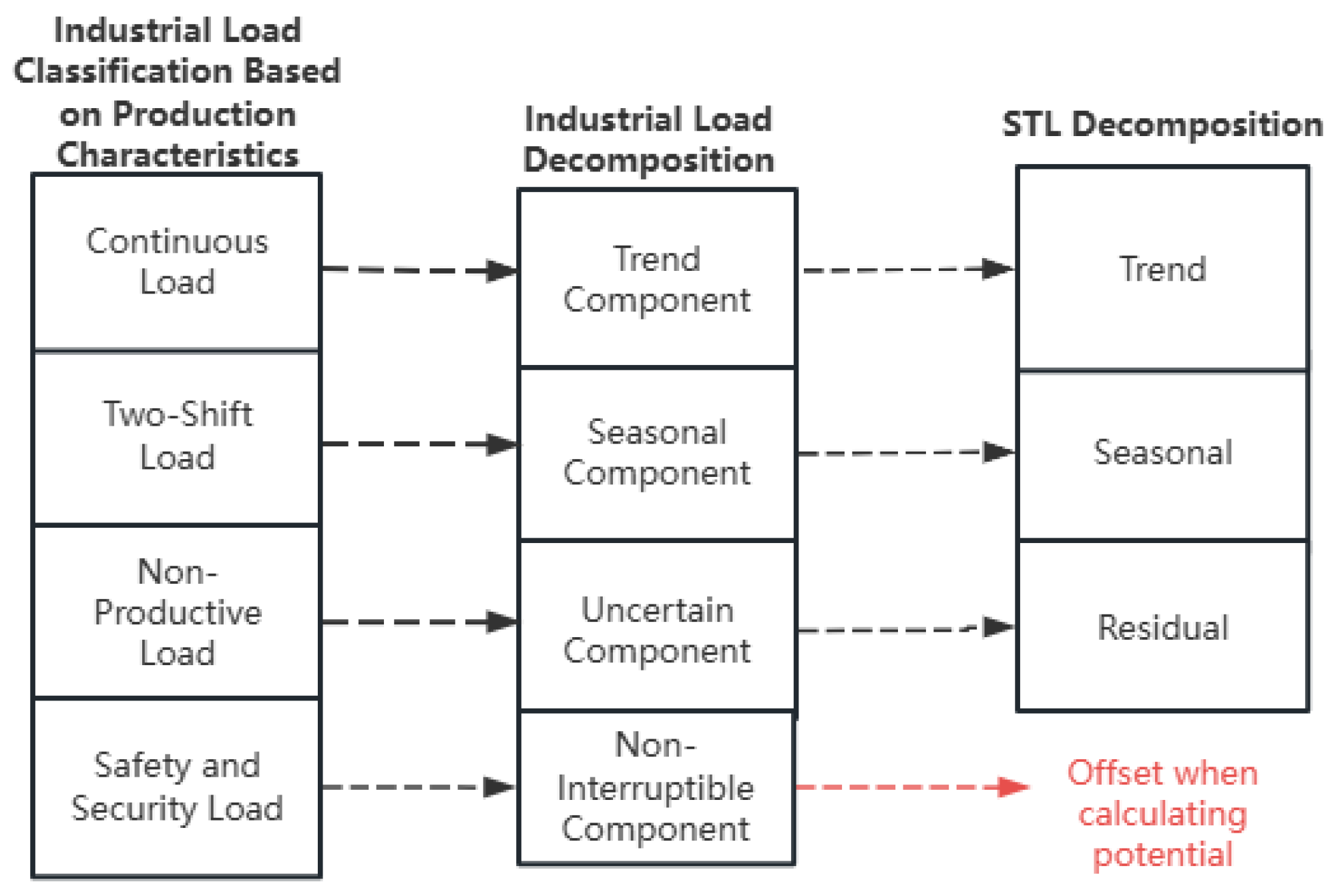
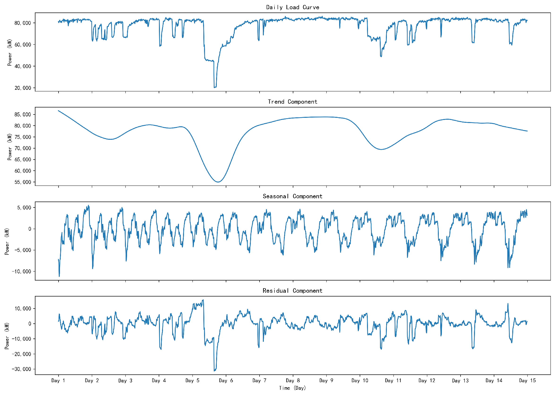
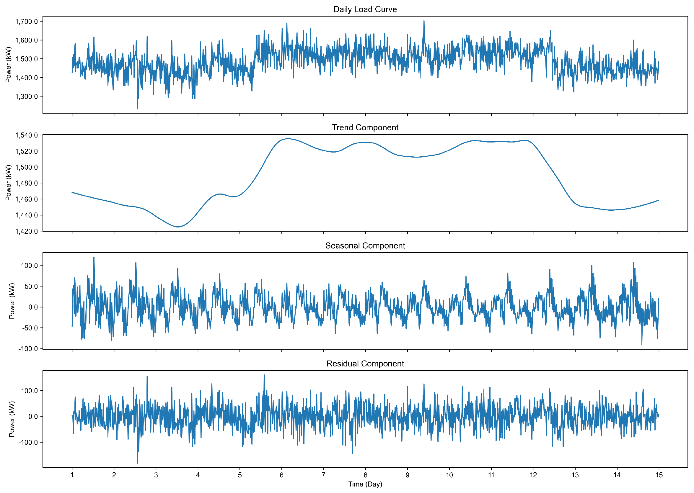
2.1. STL-Based Time-Series Feature Extraction for Industrial Users

A refined analysis of the electrical load characteristics of industrial equipment is essential. According to existing studies [20], industrial loads can be categorized into four types according to their controllability characteristics:

• Loads that allow continuous adjustment through control systems;
• Loads that support only binary on/off control and cannot be adjusted during operation;
• Loads affected by unplanned external disturbances;
• Rigid loads that must operate continuously and can only be interrupted during scheduled maintenance or adjustments.

Focusing on adjustable potential, industrial equipment can further be classified into two categories: intermittent production and continuous production types. For batch production equipment, flexibility arises primarily from shifting production schedules—by relocating energy-intensive processes to off-peak or mid-peak electricity price periods. Continuous production equipment can gain flexibility through dynamic product structure optimization—for example, prioritizing the production of low-energy-consuming products during peak price periods and switching to high-energy-consuming products during other times [21].

Based on this classification, this study proposes a four-component decoupled load model for industrial users:

• Trend Component: Represents baseline load driven by production scale, mainly associated with continuously adjustable equipment; its amplitude exhibits near-linear changes with production capacity.
• Seasonal Component: Captures fluctuations caused by periodic switching of equipment groups within the production process, often exhibiting step-like transitions on multiple intra-day timescales.
• Irregular Component: Accounts for stochastic load variations due to unplanned disturbances such as equipment failures or order changes.
• Non-interruptible Component: Reflects base load essential for safe production, which is not interruptible within a single day.

Since the demand response capacity is defined as the difference between the baseline and actual load during the demand response event period, the non-interruptible load component can be excluded from the analysis. Therefore, we focus on evaluating the trend, seasonal, and irregular components.

The Seasonal-Trend decomposition using Loess (STL) is a widely adopted technique for time-series analysis. STL was chosen due to its robustness in separating trend and seasonal components in noisy, non-stationary industrial load time series [22]. Compared with Empirical Mode Decomposition (EMD), STL offers better interpretability and avoids the mode-mixing problem. Although advanced methods such as Ensemble EMD or Variational Mode Decomposition (VMD) offer improved adaptability, they require careful tuning of parameters and often lack clear physical correspondence with industrial production behaviors, which is crucial for interpretable DR modeling. For industrial users, the time scale is usually based on 15 days, taking into account the needs of the STL decomposition algorithm and baseline calculations. It decomposes a time-series signal into three additive components: trend, seasonality, and residual [23].

Specifically, the STL algorithm decomposes the original time-series $y\left(t\right)$ as follows:

$$y\left(t\right)=T\left(t\right)+S\left(t\right)+R\left(t\right),$$

(1)

in which $T\left(t\right)$ denotes the trend component, $S\left(t\right)$ the seasonal component, and $R\left(t\right)$ the residual component.

Based on the principles of load decomposition and Equation (1), the components obtained from the STL algorithm correspond directly to the load characteristics in industrial user analysis: the trend component aligns with the trend-related load, the seasonal component reflects the periodic load fluctuations, and the residual component represents the uncertainty-induced load variations. This correspondence is illustrated as Figure 1. Accordingly, it is intuitive and reasonable to apply the STL algorithm for decomposing historical electricity consumption profiles of industrial users.

Since the residual component primarily reflects fluctuations outside of scheduled production plans, it is excluded from further analysis. Instead, feature extraction is performed on the trend and seasonal components. The resulting time-series features include the production trend factor on the demand response day and the load step matrix, both of which characterize the industrial user’s potential for flexible adjustment.

2.1.1. Production Trend Factor

The production trend factor on the response day is estimated based on the trend component of the user’s load profile over the past $n_r$ days. Specifically, the STL algorithm is applied to decompose the historical load curves (sampled at 15 min intervals) of the $n_r$ days preceding the response day, extracting the trend component $T\left(t\right)=\{T_{1,1},\dots ,T_{1,96},T_{2,1},\dots ,T_{n_r,96}\}$.

For each day, the average of the 96 trend values is computed and denoted as $e_i$, where $i=1,2,\dots ,n_r$. This yields a sequence of average trend values over the past $n_r$ days: $E_T=\{e_1,e_2,\dots ,e_{n_r}\}$($n_r\ge 15$). To quantify the relative production level on the response day, a normalized production trend factor $\theta$ is defined as

$$\theta ={\displaystyle \frac{e_1-min\{e_1,e_2,\dots ,e_{n_r}\}}{\frac{1}{n_r}{\sum }_{k=1}^{n_r}{e}_k-min\{e_1,e_2,\dots ,e_{n_r}\}}},$$

(2)

in which $e_t$ represents the trend load average on the response day.

A higher value of $\theta$ indicates a larger production scale. When $\theta >1$, it reflects an increasing trend in production activity, while $\theta <1$ indicates a decreasing trend relative to recent historical levels.

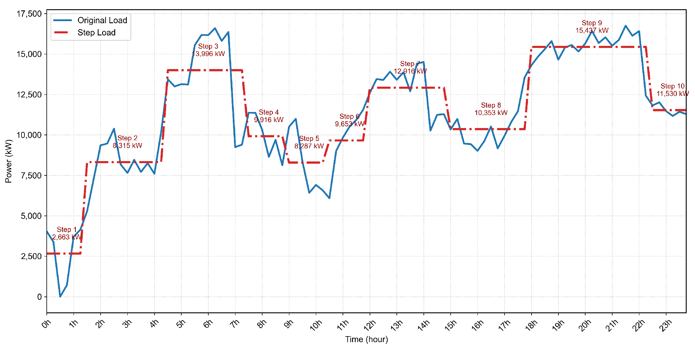
2.1.2. Load Step Matrix

Load steps accurately characterize the relatively stable operating states of industrial users, and the differences in load levels between steps reflect the theoretical potential for power adjustment arising from energy consumption variations within the production process. It is important to note that this potential refers to theoretical adjustability, not actual response behavior. Building upon the work in [19], this section proposes a formal mathematical definition of load steps and presents an algorithm for extracting the load step matrix.

A load step is defined as a quasi-steady segment in the periodic component of an industrial user’s daily load curve, with a duration longer than 1 h and a local variation rate below a specified threshold.

The local variation rate $\alpha$ is defined as

$$\alpha ={\displaystyle \frac{\Delta p_{max}-\Delta p_{\mathrm{mean}}}{\Delta p_{\mathrm{std}}}},$$

(3)

$$\Delta p_{max}=p_{max}-p_{min},$$

(4)

in which p represents the load values within a local data window, and $\Delta p$ denotes the difference between two adjacent sampling points. The operators min, max, mean, and std, respectively, refer to the minimum, maximum, mean, and standard deviation within the local window.

Typically, a local variation rate threshold $\alpha <3$ is adopted as the criterion for identifying load steps. According to the findings in [19], the load difference sequence $\{\Delta p\}$—extracted from 15 days of historical load data sampled at 15 min intervals—approximately follows a Gaussian distribution. Under this assumption, a load step corresponds to a stable operational state, where the variation in load $\{\Delta p_{max}\}$ remains within the normal fluctuation range of the overall difference sequence $[0,p_{mean}+3\Delta p_{std}]$. When $\alpha \ge 3$, the load fluctuation exceeds this range, indicating that the user has transitioned from a steady state to a transient operating condition.

From a physical perspective, transitions between load steps are primarily caused by shifts in the operational states of clustered industrial equipment, resulting in step changes in load levels. Typical scenarios include the startup or shutdown of energy-intensive machinery and switching between production line modes.

From a mathematical perspective, the identification of load steps focuses on steady-state segments by discarding transient data between steps. For each selected segment, the algorithm retains the average load value, start time, and end time, which together represent the essential characteristics of the load step. An illustration of load steps is shown in Figure 2.

Figure 2 illustrates an example of an industrial user’s daily load profile sampled every 15 min. The blue solid line represents the actual periodic component of the original load curve, and the red dashed line shows the processed curve after load step extraction.

Using 15 min sampling data from the 15 days prior to the response day and a sliding window of duration $T=1 \mathrm{h}$, the load step extraction process is as follows:

• Apply the STL algorithm to the historical load data to obtain the periodic load component:

  $$S_r=\{S_{1,1},\dots ,S_{1,96},S_{2,1},\dots ,S_{n_r,96}\},r\in [1,15],$$

  (5)
• Initialize the load step candidate buffer $\alpha$ with the first four load points in $S_r$, and set the threshold $\alpha <3$ as the criterion for a valid load step:

  $$\alpha =S_r[1,2,3,4],$$

  (6)
• Iterate through the periodic load sequence $S_r$ to identify load steps using the following rule:

  $$\alpha =\left\{\begin{array}{cc}[\alpha ,S_r\left(t\right)],\hfill & \alpha <3\hfill \\ \left[S_r[t-3,t]\right],\hfill & \alpha \ge 3\hfill \end{array}\right.,$$

  (7)
  The position index t is updated accordingly. Initialize $t=5$. If $S_r\left(t\right)$ belongs to the same load step as $S_r(t-1)$, increment t by 1. If only one of them belongs to a valid step, also increment t. Otherwise, increment t by 1 to continue traversal.
• For each identified load step, record its characteristics as

  $$P_j\left(t\right)=\{p_{j,1}\left(t\right),p_{j,2}\left(t\right),p_{j,3}\left(t\right)\},j\in [1,n_t],$$

  (8)

  where $p_{j,1}\left(t\right)$, $p_{j,2}\left(t\right)$, and $p_{j,3}\left(t\right)$ denote the start time, end time, and average load of the j-th step, respectively, extracted from the original periodic load component.
• The extracted load step matrix for day t is denoted as

  $$T_t=[P_1\left(t\right);P_2\left(t\right);\dots ;P_{n_t}\left(t\right)],t\in [1,15],$$

  (9)

In summary, the full load step matrix T over the past 15 days is given by

$$T=[T_1;T_2;\dots ;T_{15}],$$

(10)

2.2. Response Feature Analysis Based on Historical Demand Response Invitations

In addition to the aforementioned time-series features, a user’s willingness to participate in DR programs is also a critical factor influencing their overall response potential [24]. This paper proposes five quantitative indicators to capture the user’s DR willingness characteristics, based on historical electricity consumption records, past DR participation data, and user-submitted response information on the target response day.

2.2.1. Historical Declared Participation Rate

To quantify a user’s historical responsiveness to DR invitations, we introduce the Historical Declared Participation Rate ($R_{\mathrm{his}}$). This metric represents the proportion of past DR events in which the user declared participation relative to all received invitations. The formal calculation is expressed as follows:

$$R_{\mathrm{his}}={\displaystyle \frac{1}{M}}\sum _{k=1}^M{r}_k,$$

(11)

where $R_{\mathrm{his}}$ is the user’s historical declaration participation rate. M is the total number of past DR invitations, and $r_k$ indicates whether the user responded to the k-th invitation ($r_k=1$ if participated, $r_k=0$ otherwise).

2.2.2. Historical Effective Response Rate

To quantify the historical reliability of a user’s actual demand response performance, we introduce the Historical Effective Response Rate ($E_{\mathrm{his}}$). This metric represents the proportion of past DR events where the user successfully met the predetermined effectiveness criteria. The formal calculation is expressed as follows:

$$E_{\mathrm{his}}={\displaystyle \frac{1}{M}}\sum _{i=1}^M{q}_i,$$

(12)

where $E_{\mathrm{his}}$ is the user’s historical effective response rate. $q_i$ indicates whether the user met the effective response criteria for the i-th DR event ($q_i=1$ if yes, $q_i=0$ otherwise). A response is considered effective if it satisfies both: (1) the maximum reduction in the DR time window exceeds the baseline load as explained in Section 3.1; (2) the average reduction is no less than 50% of the declared response capacity.

2.2.3. Industry-Relative Factor

To evaluate the relative contribution of a specific industry in historical demand response (DR) events, we introduce the Industry-Relative Factor ($D_{k,\mathrm{his}}$). This index quantifies the average proportion of total DR response volumes attributable to industry k across all past DR events. The formal calculation is expressed as follows:

$$D_{k,\mathrm{his}}={\displaystyle \frac{1}{M}}\sum _{j=1}^M{\displaystyle \frac{y_{k,j}}{Y_j}},$$

(13)

where $D_{k,\mathrm{his}}$ is the industry-relative factor index for industry k. $y_{k,j}$ is the DR response volume from industry k during the j-th event, and $Y_j$ is the total response volume for the j-th event.

2.2.4. Relative Declared Response Volume

To assess the proportionality between a user’s declared demand response commitment and their actual capabilities, we introduce the Relative Declared Response Volume ($C_{\mathrm{rec}}$). This ratio measures the declared response capacity against the user’s maximum achievable load reduction potential under normal operating conditions. The formulation is defined as follows:

$$C_{\mathrm{rec}}={\displaystyle \frac{c_r}{c}},$$

(14)

where $C_{\mathrm{rec}}$ is the ratio of declared response capacity $c_r$ to the user’s maximum DR potential c under normal conditions.

2.2.5. Invitation-to-Declared Price Ratio

$$P_{\mathrm{rec}}={\displaystyle \frac{P_r}{P_{max}}},$$

(15)

where $P_{\mathrm{rec}}$ is the ratio of the user’s declared response price $P_r$ to the DR invitation upper-limit price $P_{max}$ provided by the power company.

2.2.6. Feature Vector Summary

Finally, the user’s comprehensive DR feature vector is expressed as

$$x_i=[{\theta }_i,T_i,R_{\mathrm{his},i},E_{\mathrm{his},i},D_{k,\mathrm{his},i},C_{\mathrm{rec},i},P_{\mathrm{rec},i}],$$

(16)

where ${\theta }_i$ denotes the normalized production trend factor, $T_i$ represents the load step matrix features, and the remaining five variables characterize the user’s historical response willingness from different behavioral and economic perspectives.

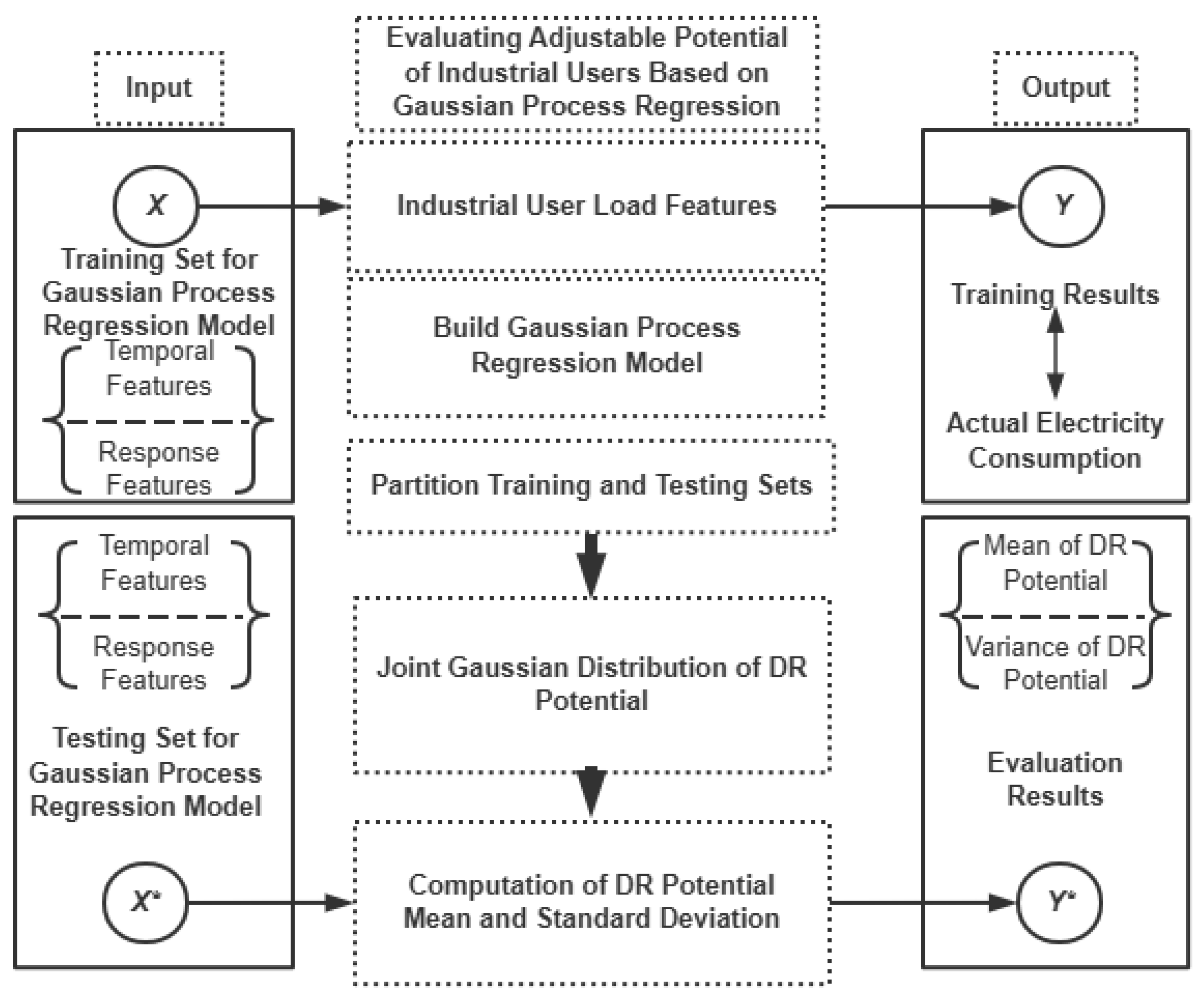
3. Industrial Demand Response Potential Estimation Based on Gaussian Process Regression

This study focuses on incentive-based demand response programs. The effective demand response load is defined as the difference between the baseline average load and the actual average load during the declared response period. The demand response potential is calculated as follows:

$$P_{\mathrm{DR}}=\overline{P_T}-\overline{P_A},$$

(17)

where $P_{\mathrm{DR}}$ denotes the effective demand response load, $\overline{P_T}$ represents the baseline average load during the demand response period, and $\overline{P_A}$ is the actual average load observed during the same period.

Section 3.1 elaborates on the baseline calculation methodology, while Section 3.2 presents the demand response energy evaluation based on Gaussian Process Regression.

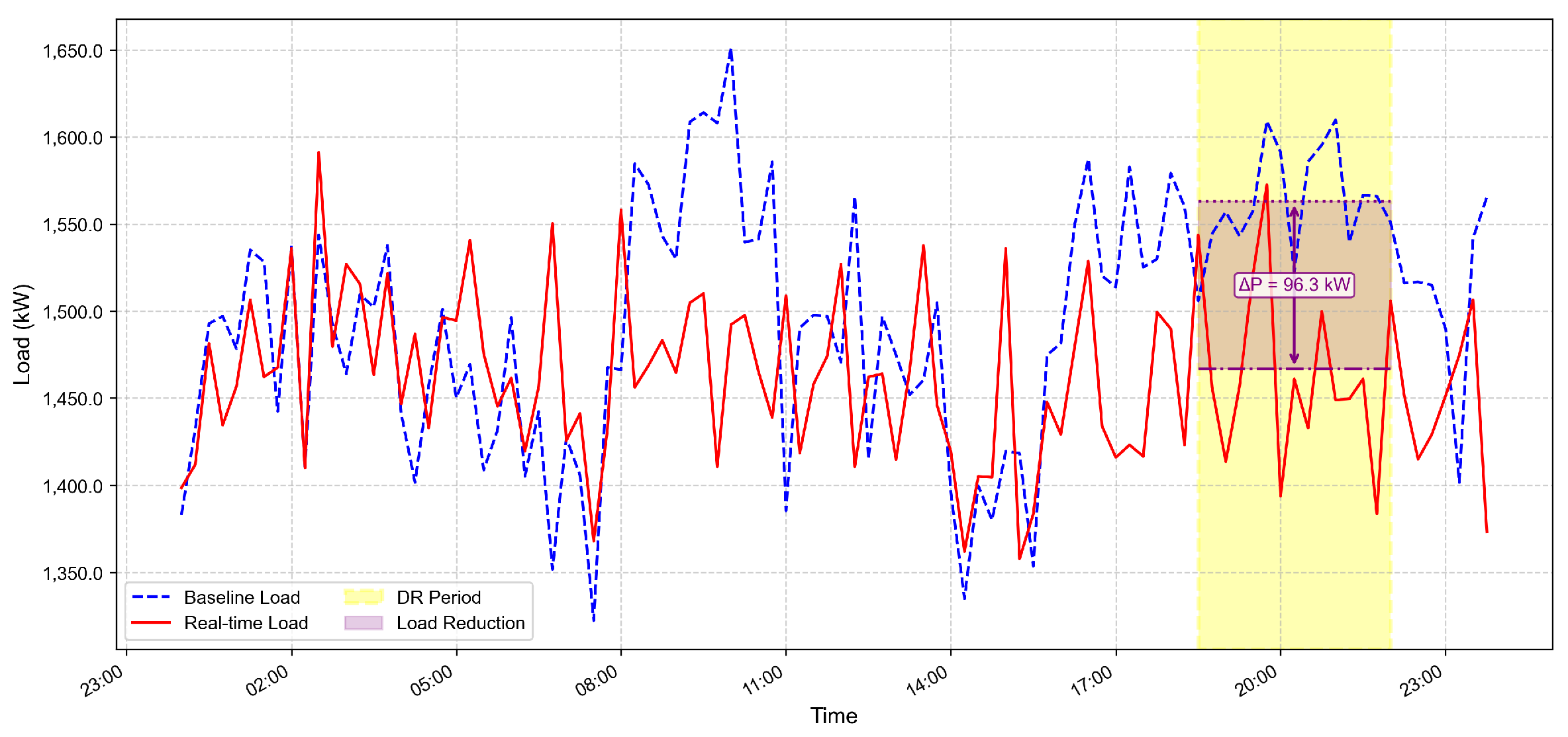
3.1. Baseline Estimation Based on Historical Load Data

The baseline is derived from the trend component of the load curve on selected sample days prior to the DR event, extracted using the STL algorithm. The maximum load observed in the baseline is referred to as the baseline peak load, while the arithmetic mean of the baseline load is defined as the baseline average load. For users who participate in DR events on both weekdays and non-weekdays, separate baselines are calculated for each category [25].

3.1.1. Weekday Baseline

The selection criteria for weekday baseline samples are as follows. Using the DR event day as the reference, the five most recent valid weekdays (excluding weekends, national holidays, and previous DR event days) are chosen to form the initial sample set. Outliers are removed based on the daily average load $\mu$ of the initial set, excluding any day for which $\mu <0.25\overline{\mu }$ or $\mu >2\overline{\mu }$.

If fewer than five valid samples remain after outlier removal, backward replacement is performed in reverse chronological order within a 30-day window preceding the reference day. The replacement process stops when either of the following conditions is met:

(a)

Five qualified sample days are obtained;

(b)

The search exceeds 30 calendar days.

Once n sample days are selected, the STL algorithm is applied to extract the trend component from each day’s load curve. For each 15 min interval across the 24 h period (96 intervals per day), the average load value is calculated as

$$\overline{P_T}={\displaystyle \frac{1}{n}}\sum _{i=1}^n{p}_{i,t},$$

(18)

where $\overline{P_T}$ denotes the baseline load at time interval t, and $p_{i,t}$ is the trend component at interval t on sample day i.

3.1.2. Non-Weekday Baseline

For non-weekday baselines, the selection procedure is similar but adapted to weekends or holidays. The three most recent non-working days, excluding weekdays and historical DR days, are chosen to form the initial sample set. Outlier filtering is applied using the same criterion as the weekday case: days satisfying $\mu <0.25\overline{\mu }$ or $\mu >2\overline{\mu }$ are removed.

If fewer than three valid samples remain, backward replacement is conducted within a 30-day window. The process is terminated when

(a)

Three qualified sample days are obtained;

(b)

The search exceeds 30 calendar days.

Once n valid sample days are selected, the baseline is computed using Equation (18).

3.2. Power Consumption Estimation in DR Period Based on Gaussian Process Regression

In practical grid dispatching, apart from the estimated DR potential of individual users, it is also essential to quantify the uncertainty associated with users who exhibit similar potential values. This uncertainty measure can serve as an important input to assist scheduling decisions. Gaussian Process Regression (GPR), a non-parametric regression method rooted in Bayesian statistical theory, provides both function predictions and associated uncertainty estimates by modeling the unknown function as a Gaussian process [26].

Following the findings in [27], the DR potential of industrial users is assumed to follow a Gaussian distribution. Since the DR potential is computed as the difference between the actual load during the DR execution period and the baseline load, the actual load itself is also assumed to follow a Gaussian distribution.

Given that a Gaussian process is defined as a collection of random variables, any finite subset of which follows a joint Gaussian distribution, the joint distribution of actual loads from infinitely many DR periods can be modeled as a Gaussian process [28]. Therefore, a GPR model can be employed to learn the mapping between industrial user features and electricity consumption during DR periods.

3.2.1. Gaussian Kernel Function

In the GPR framework, the bandwidth parameter $\sigma$ of the kernel function is a crucial hyperparameter that governs the generalization performance of the model. This parameter adjusts the decay behavior of the covariance function, thereby influencing the similarity measure between samples. Specifically,

• As $\sigma \to 0$, the covariance matrix approximates the identity matrix, and the model captures only highly localized features;
• As $\sigma \to \infty$, the covariance matrix converges to a matrix of ones, and the model degenerates into a global mean predictor.

Quantitatively, the impact of the bandwidth parameter on model performance is represented by

$$K(x_i,x_j)=exp\left(-{\displaystyle \frac{\parallel x_i-x_j{\parallel }^2}{2{\sigma }^2}}\right),$$

(19)

where $x_i$ and $x_j$ are input feature vectors, and $\parallel x_i-x_j\parallel$ denotes the Euclidean distance between them. The parameter $\sigma$ reflects the rate of similarity decay in feature space.

According to the Vapnik–Chervonenkis (VC) dimension theory, an excessively small value of $\sigma$ leads to high hypothesis space complexity, resulting in overfitting characterized by low training error and high testing error. Conversely, a large $\sigma$ compresses the effective dimensionality of the hypothesis space, causing underfitting.

To tune $\sigma$ and assess model robustness, this study adopts K-fold cross-validation. The dataset is partitioned into K equally sized subsets. In each iteration, $K-1$ subsets are used for training, while the remaining one is used for validation. This method provides a more stable and reliable evaluation of model performance compared to single-fold validation. The validation procedure is detailed in Algorithm 1.

Algorithm 1 K-fold cross-validation procedure for demand response potential estimation.

Require:  Dataset $D={\left\{(x_i,y_i)\right\}}_{i=1}^N$, number of folds $K\in {\mathbb{N}}^{+}$ Ensure:  Model performance metric $\mu \pm \sigma$   1: Step 1: Data Partitioning   2: Split D into K mutually exclusive subsets: $D_1,D_2,\dots ,D_K$,   3: such that ${\bigcap }_{k=1}^K{D}_k=\varnothing$ and ${\bigcup }_{k=1}^K{D}_k=D$   4: Step 2: Iterative Validation   5: for $k\leftarrow 1$ to K do   6:       Construct training set $T_k={\bigcup }_{j\ne k}{D}_j$   7:       Set validation set $V_k=D_k$   8:       Train GPR model $M_k\left(\theta \right)$ on $T_k$ (where $\theta$ denotes hyperparameters)   9:       Compute validation performance metric ${\epsilon }_k=\mathrm{MAE}(M_k,V_k)$ 10: end for 11: Step 3: Performance Evaluation 12: Compute mean performance: $\mu ={\displaystyle \frac{1}{K}}{\sum }_{k=1}^K{\epsilon }_k$ 13: Compute standard deviation: $\sigma =\sqrt{{\displaystyle \frac{1}{K-1}}{\sum }_{k=1}^K{({\epsilon }_k-\mu )}^2}$ 14: Step 4: Return Results 15: return Final performance metric $\mu \pm 1.96\sigma$

3.2.2. Gaussian Process Regression Model for Demand Response Energy Estimation

This section models the mapping between industrial user features and actual electricity consumption during DR periods using a GPR framework. The target function is modeled as a Gaussian process with a Gaussian prior distribution, and its parameters are treated as random variables.

Let the training dataset for actual load estimation during DR periods be denoted by

$$\mathcal{D}=\left\{(x_i,y_i)\right|i=1,2,\dots ,n\}=\{X,y\},$$

(20)

where n is the number of DR-participating users in the training set, $X\in {\mathbb{R}}^{n\times d}$ is the input matrix of user feature vectors, and $y\in {\mathbb{R}}^n$ is the vector of actual electricity consumption in the DR period for each user.

The joint distribution of $\mathcal{D}$ follows a multivariate Gaussian distribution, uniquely defined by the mean function $\mu \left(X\right)$ and covariance matrix $K(X,X)$:

$$y\sim \mathcal{GP}\left(\mu \right(X),K(X,X\left)\right)$$

(21)

In practice, the observed consumption includes Gaussian noise:

$${\tilde{y}}_i=y_i+{ϵ}_i,{ϵ}_i\sim \mathcal{N}(0,{\sigma }_n^2),$$

(22)

Hence, the prior becomes

$$y\sim \mathcal{N}(\mu \left(X\right),K(X,X)+{\sigma }_n^{2}I),$$

(23)

To evaluate model performance, a separate test set is defined as

$${\mathcal{D}}^{*}=\left\{(X^{*},y^{*})\right\},X^{*}\in {\mathbb{R}}^{m\times d},y^{*}\in {\mathbb{R}}^m,$$

(24)

The joint prior distribution over training and test outputs is given by

$$\left[\begin{array}{c}y\\ y^{*}\end{array}\right]\sim \mathcal{N}\left(\left[\begin{array}{c}\mu \left(X\right)\\ \mu \left(X^{*}\right)\end{array}\right],\left[\begin{array}{cc}K(X,X)+{\sigma }_n^{2}I& K(X,X^{*})\\ K(X^{*},X)& K(X^{*},X^{*})\end{array}\right]\right),$$

(25)

The kernel function used in this model is a Gaussian kernel as (19). From Bayesian inference, the predictive distribution of the test outputs is

$${\widehat{y}}^{*}=\mu \left(X^{*}\right)+K(X^{*},X){[K(X,X)+{\sigma }_n^{2}I]}^{-1}(y-\mu \left(X\right)),$$

(26)

$${\sigma }_y^2*=K(X^{*},X^{*})-K(X^{*},X){[K(X,X)+{\sigma }_n^{2}I]}^{-1}K(X,X^{*}).$$

(27)

For a 95% confidence interval, the predictive result lies in

$$y_i\in \left[\overline{y_{i^{*}}}-1.96{\sigma }_{y_{i^{*}}},\overline{y_{i^{*}}}+1.96{\sigma }_{y_{i^{*}}}\right],i=1,2,\dots ,n$$

(28)

Finally, using the industrial user load feature vector $x_i$ defined in Equation (16) as input, the GPR-based industrial DR potential estimation framework is illustrated in Figure 3.

4. Case Study Analysis

To verify the effectiveness of the proposed quantitative assessment method for industrial user DR potential, a case study is conducted using real data from a peak-shaving DR event in a province of China in 2022. The DR invitation period lasted from 17:00 to 22:00, involving 198 industrial users. The dataset includes the following:

• Historical electricity consumption data for the 15 weekdays prior to the response day;
• Historical DR participation records;
• DR registration data submitted by users.

All data were collected at 15 min intervals.

Section 4.1 presents the load feature extraction results for two representative types of industrial users. Section 4.2 evaluates the overall accuracy of the proposed DR potential assessment method and compares it with other mainstream approaches.

4.1. Load Feature Extraction for Industrial Users

An analysis of historical response data as Figure 4 reveals that five sectors dominate adjustable loads during midday and evening peak periods: (i) the chemical raw material and chemical product manufacturing industry (16.05%), (ii) computer, communication, and other electronic equipment manufacturing (12.97%), (iii) non-metallic mineral products (8.34%), (iv) ferrous metal smelting and rolling (6.40%), and (v) automobile manufacturing (5.84%).

These five sectors together account for approximately half of the total peak-shifting capacity. Among them, the chemical manufacturing industry exhibits strong potential during seasonal peaks due to its preference for off-peak electricity, especially enabling it to avoid the 20:00–22:00 high-price window during summer and winter peaks.

By contrast, high-value-added industries such as computer and electronics manufacturing are less price-sensitive and thus less responsive to DR incentives. To illustrate this difference, we select one chemical enterprise and one high-tech enterprise for comparative analysis.

4.1.1. Load Feature Extraction for a Chemical Enterprise

The historical load data from the 15 weekdays prior to the DR event for this chemical enterprise were decomposed using the STL algorithm. The decomposition results are shown in Figure 5. Based on the trend component, the production trend factor was calculated as 1.59, which is greater than 1, indicating an upward trend in production activity compared to the 15-day average.

Since load steps are defined based on differences in load values, the periodic component on the response day was zero-calibrated at midnight before extracting step segments. The resulting load step profile is illustrated in Figure 6.

According to historical DR records, the user exhibits strong willingness to participate in demand response, with the following indicators:

• Historical Declaration Participation Rate: 0.63;
• Historical Effective Response Rate: 1.00;
• Industry-relative Value Added: 0.16;
• Relative Declared Response Volume: 0.56;
• Price Ratio: 1.00.

These values collectively indicate a high level of responsiveness and self-awareness of flexibility potential for this user. Based on the GPR model, the DR potential for this chemical enterprise was estimated. The predicted potential follows a Gaussian distribution with a mean of 11,741.39 kW and a standard deviation of 851.23 kW. Under a 95% confidence level, the DR potential confidence interval is calculated as [10,072.98 kW, 13,409.80 kW].

As illustrated in Figure 7, the user achieved an actual load reduction of 13,070.80 kW during the test period. This value falls within the upper range of the confidence interval, providing empirical evidence for the reliability of the proposed model in evaluating highly responsive users.

Notably, the load-monitoring data revealed a significant difference between the maximum and minimum load steps, reaching 12,773.83 kW, as shown in Figure 6. For chemical industry users characterized by high interruptibility, this difference not only reflects the volatility in equipment operation but also serves as a valuable prior indicator for estimating potential DR capacity.

In this case study, the user’s actual load adjustment achieved 102.32% of the maximum load step difference. This further confirms the user’s strong load adjustment flexibility and high DR execution efficiency.

4.1.2. Load Feature Extraction for a High-Tech Enterprise

The historical load data from the 15 weekdays prior to the DR event were decomposed using the STL algorithm, with the results shown in Figure 8. From the trend component, the production trend factor was calculated as 0.72, which is less than 1, indicating a downward trend in production compared to the 15-day average.

Since load steps are defined based on differences in load values, the periodic component on the response day was zero-calibrated at midnight before extracting step segments. The extracted load steps are illustrated in Figure 9.

According to historical DR data, this user exhibited relatively weak willingness to participate in demand response, with the following feature indicators:

• Historical Declaration Participation Rate: 0.27;
• Historical Effective Response Rate: 0.50;
• Industry-relative Value Added: 0.02;
• Relative Declared Response Volume: 0.06;
• Price Ratio: 0.25.

The GPR model was used to estimate the user’s DR potential. The resulting distribution had a mean of 91.42 kW and a standard deviation of 3.88 kW. Under a 95% confidence level, the confidence interval was computed as [83.82 kW, 99.02 kW].

As shown in Figure 10, the user achieved an actual load reduction of 96.31 kW during the test period, which lies in the upper range of the confidence interval. This result demonstrates that the GPR model remains effective even for users with weak DR willingness.

It is worth noting that despite being classified as only moderately interruptible and weakly responsive, this user’s maximum-to-minimum load step difference still reached 76.74 kW in Figure 9. In this case, the actual response reached 125.50% of the maximum load step difference.

This observation reveals that even for user groups with relatively low DR potential, the load step difference serves as a fundamental indicator of their physical flexibility; while actual response behavior is constrained by willingness to participate, the load step difference offers an objective reflection of the underlying adjustable capacity on the user side. The case studies across multiple user types demonstrate that the load step difference serves as a generally applicable indicator in DR potential assessment. For users with high response willingness (e.g., chemical enterprises), the load step difference can be directly mapped to achievable regulation capacity. In contrast, for users with low response willingness (e.g., high-tech enterprises), this parameter represents the upper bound of their physical regulation capability. These findings further validate the role of response willingness indicators in assessing the DR potential of industrial users.

4.2. Effectiveness Verification of the Industrial DR Potential Evaluation Method

To verify the accuracy of the proposed DR potential evaluation method, we define an evaluation accuracy metric Z, as shown in Equation (29). This metric represents the ratio of the number of users whose DR potential is accurately assessed to the total number of users participating in the DR invitation.

$$Z={\displaystyle \frac{1}{n}}\sum _{i=1}^n{z}_i,$$

(29)

Here, $z_i=1$ indicates one of two conditions:

• The actual DR response of user i is less than zero, and the mean predicted DR value by the Gaussian Process Regression model is also less than zero—i.e., the model correctly predicted the user would not participate in DR;
• The actual DR response of user i falls within the 95% confidence interval predicted by the model, expressed as Equation (28).

Otherwise, $z_i=0$.

To validate the necessity of incorporating DR willingness indicators in the proposed evaluation model, a controlled experiment was conducted. As shown in

Table 2. Accuracy comparison with and without considering DR willingness.

User ID	Actual Response (kW)	with DR Willingness			Without DR Willingness
		Mean (kW)	Std Dev (kW)	${\mathit{z}}_{\mathit{i}}$	Mean (kW)	Std Dev (kW)	${\mathit{z}}_{\mathit{i}}$
1	1970.63	1930.82	27.17	1	1905.60	30.88	0
2	836.35	807.18	19.23	1	816.21	21.15	1
3	2152.97	2104.89	39.88	1	2189.32	43.81	1
4	13,070.80	11,741.39	851.23	1	12,902.34	883.18	1
⋮	⋮	⋮	⋮	⋮	⋮	⋮	⋮
196	30,272.19	27,615.06	905.02	0	28,133.22	932.14	0
197	113.38	115.02	2.11	1	90.89	2.99	0
198	68.05	68.88	1.72	1	71.77	2.32	1
Z				91.4%			57.1%

, when using the GPR model that integrates DR willingness features, the evaluation accuracy Z reached 91.4%—correctly predicting the actual response behavior of 181 out of 198 users, including both those whose behavior was covered by the 95% confidence interval and those who did not participate.

In contrast, when the willingness indicators were excluded from the model, the accuracy Z dropped significantly to 57.1%, correctly predicting only 113 of the 198 users. This sharp decline highlights the critical explanatory role of user response willingness in DR potential estimation.

In industrial user scenarios, the physical adjustability inferred from load time-series features constitutes only a necessary condition for DR potential. However, the actual realization of this potential is largely dependent on users’ willingness to participate, which is influenced by economic incentives, production schedules, and operational constraints. Therefore, willingness serves as a sufficient condition that determines the effective transformation of theoretical potential into realized response.

To further demonstrate the superiority of the proposed evaluation method over existing DR potential assessment approaches, a comparative analysis was conducted under the condition of equal data granularity. Two commonly used evaluation metrics—Mean Absolute Percentage Error (MAPE) and Root Mean Squared Error (RMSE)—were employed to compare the performance of the proposed model with two benchmark DR potential estimation methods.

The first benchmark is a two-stage clustering-based method, which extracts user typical patterns by constructing user features. The DR potential is then estimated as the difference between the user’s maximum load on a representative day and the average load during the response period.

The second benchmark is a deep subdomain adaptation-based method, which constructs a library of quadratic regression parameters for user load patterns. Based on this library, DR potential is evaluated using parameter similarity to estimate users’ response capabilities. The comparison results are shown in Figure 11.

As shown in Figure 11, the proposed GPR-based method for evaluating industrial users’ DR potential exhibits clear advantages over benchmark approaches. Specifically, the conventional two-stage clustering method [29], while computationally efficient and suitable for rough estimations in engineering scenarios, results in relatively large evaluation errors, which limits its applicability in precision dispatching tasks by power companies.

The adaptive learning-based method [14] improves accuracy by incorporating user similarity analysis mechanisms. However, it still fails to fully capture the dynamic nature of user willingness and the load characteristics of specific DR invitation periods. As a result, for industrial users with similar load patterns, the MAPE remains 16.4 percentage points higher on average than that of the proposed GPR method.

It is worth noting that both benchmark methods output deterministic estimates of DR potential, whereas the proposed GPR-based method provides a probabilistic distribution. In real-world applications, such as dispatch planning by power companies or load aggregators, confidence intervals of the estimated response volume can help stakeholders understand both the expected response and its associated uncertainty. This enables the development of risk-informed and robust dispatch strategies.

Importantly, the probabilistic nature of the proposed GPR framework introduces a trade-off between precision and interpretability, while uncertainty quantification enables robust planning under variability, it may also pose challenges to operators unfamiliar with confidence-based decision models.

To address this, we advocate for the integration of Bayesian Decision Theory (BDT) in future extensions of the proposed framework. In BDT, the optimal action $a^{*}$ (e.g., DR commitment level) is determined by maximizing the expected utility:

$$a^{*}=arg\underset{a\in \mathcal{A}}{max}\int u(a,y)p(y\mid \mathbf{x})dy,$$

(30)

where $u(a,y)$ is the utility function representing dispatch goals (e.g., reliability or cost-efficiency), and $p(y\mid \mathbf{x})$ is the predictive distribution output from GPR.

This formulation allows system operators to rationally hedge against over- or under-commitment risks in DR resource scheduling. In essence, it transforms probabilistic forecasts into actionable, risk-informed decisions, bridging the gap between machine learning models and operational feasibility.

The case study demonstrates that the proposed approach significantly enhances the granularity and reliability of DR potential assessment. This technical advantage mitigates scheduling mismatches caused by estimation errors and supports rational capacity allocation and effective execution of DR dispatch instructions—both of which are essential for the success of DR bidding and implementation in power markets.

5. Conclusions

To address the challenges of low accuracy and limited uncertainty characterization in industrial DR potential evaluation, this paper proposes a novel GPR framework that integrates STL decomposition and load step features. By decomposing load curves into trend and periodic components and incorporating a response willingness feature system derived from historical participation behavior, the proposed method enables high-accuracy and interpretable assessments of industrial DR potential.

Experimental results demonstrate that the method outperforms mainstream alternatives in both accuracy and uncertainty quantification. It exhibits strong generalization capabilities and adaptability in industrial load scenarios characterized by high uncertainty and heterogeneity.

Moreover, this study verifies the universality of load step difference as a physical indicator of industrial users’ regulation capability. It also highlights the critical role of response willingness in determining the actual realization of theoretical DR potential. These insights provide a theoretical foundation and practical guidance for developing more comprehensive and dynamic DR evaluation systems in the future.

In summary, the proposed method not only improves the precision of identifying industrial DR capacity but also serves as an effective tool for power system operators to better exploit and dispatch demand-side flexibility resources. Future research may extend this framework to real-time DR applications and explore flexibility coordination under multi-energy systems.

References

1. National Energy Administration. Statistical Data of China’s Electric Power Industry in 2024 [EB/OL]. 21 January 2025. Available online: https://www.nea.gov.cn/20250121/097bfd7c1cd3498897639857d86d5dac/c.html (accessed on 1 June 2025).
2. Ghafoor, A.; Aldahmashi, J.; Apsley, J.; Djurović, S.; Ma, X.; Benbouzid, M. Intelligent Integration of Renewable Energy Resources Review: Generation and Grid Level Opportunities and Challenges. Energies 2024, 17, 4399. [Google Scholar] [CrossRef]
3. Singh, S.; Singh, S. Advancements and challenges in integrating renewable energy sources into distribution grid systems: A comprehensive review. J. Energy Resour. Technol. 2024, 146, 090801. [Google Scholar] [CrossRef]
4. Paterakis, N.G.; Erdinç, O.; Catalão, J.P. An overview of Demand Response: Key-elements and international experience. Renew. Sustain. Energy Rev. 2017, 69, 871–891. [Google Scholar] [CrossRef]
5. Heffron, R.; Körner, M.F.; Wagner, J.; Weibelzahl, M.; Fridgen, G. Industrial demand-side flexibility: A key element of a just energy transition and industrial development. Appl. Energy 2020, 269, 115026. [Google Scholar] [CrossRef]
6. International Energy Agency. Cement Technology Roadmap Plots Path to Cutting CO2 Emissions 24% by 2050; IEA: Paris, France, 2018. [Google Scholar]
7. Germscheid, S.H.; Mitsos, A.; Dahmen, M. Demand response potential of industrial processes considering uncertain short-term electricity prices. AIChE J. 2022, 68, e17828. [Google Scholar] [CrossRef]
8. dos Santos, S.A.B.; Soares, J.M.; Barroso, G.C.; de Athayde Prata, B. Demand response application in industrial scenarios: A systematic mapping of practical implementation. Expert Syst. Appl. 2023, 215, 119393. [Google Scholar] [CrossRef]
9. Dai, X.; Chen, H.; Xiao, D.; He, Q. Review of applications and researches of industrial demand response technology under electricity market environment. Power Syst. Technol. 2022, 46, 4169–4186. [Google Scholar]
10. Liu, D.; Sun, Y.; Li, B.; Huo, M.L.; Xi, W.M. Price-based demand response mechanism of prosumer groups considering adjusting elasticity differentiation. Power Syst. Technol. 2020, 44, 2062–2070. [Google Scholar]
11. Nilsson, A.; Lazarevic, D.; Brandt, N.; Kordas, O. Household responsiveness to residential demand response strategies: Results and policy implications from a Swedish field study. Energy Policy 2018, 122, 273–286. [Google Scholar] [CrossRef]
12. Mari, S.; Bucci, G.; Ciancetta, F.; Fiorucci, E.; Fioravanti, A. A review of non-intrusive load monitoring applications in industrial and residential contexts. Energies 2022, 15, 9011. [Google Scholar] [CrossRef]
13. Sun, Q.; Liu, Y.; Hu, J.; Hu, X. Non-intrusive we-energy modeling based on GAN technology. Proc. CSEE 2020, 40, 6784–6793. [Google Scholar]
14. Kong, X.Y.; Liu, C.; Wang, C.S.; Li, S.W.; Chen, S.S. Demand response potential assessment method based on deep subdomain adaptation network. Proc. CSEE 2022, 42, 5786–5797. [Google Scholar]
15. Di, W.U.; Yunchu, W.A.N.G.; Chunlei, Y.U. Demand response potential evaluation method of industrial users based on Gaussian process regression. Electr. Power Autom. Equip. 2022, 42, 94–101. [Google Scholar]
16. Jiang, Z.; Lee, Y.M. Deep Transfer Learning for Thermal Dynamics Modeling in Smart Buildings. In Proceedings of the 2019 IEEE International Conference on Big Data (Big Data), Los Angeles, CA, USA, 9–12 December 2019; IEEE: Los Angeles, CA, USA, 2019; pp. 2033–2037. [Google Scholar]
17. Chen, Y.; Li, Y.; Shen, Y. Industrial customer group portrait method based on potential quantization model of load control. Electr. Power Autom. Equip. 2021, 41, 208–216. [Google Scholar]
18. Shi, J.; Wen, F.; Cui, P.; Sun, L.; Shang, J.; He, Y. Intelligent energy management of industrial loads considering participation in demand response program. Autom. Electr. Power Syst. 2017, 41, 45–53. [Google Scholar]
19. Su, X.; Lyu, R.; Guo, H.; Chen, Q. A Method for Optimal Selection of High-Capacity Industrial Users for Demand Response Based on Load Step Data Processing Mode. Electr. Power 2024, 57, 18–29. [Google Scholar]
20. Lee, E.; Baek, K.; Kim, J. Evaluation of demand response potential flexibility in the industry based on a data-driven approach. Energies 2020, 13, 6355. [Google Scholar] [CrossRef]
21. Zhu, D. Analysis and Application of Typical Load Electricity Behavior Model. Master’s Thesis, Southeast University, Nanjing, China, 2017. [Google Scholar]
22. Wu, D.; Wang, Y.; Li, L.; Lu, P.; Liu, S.; Dai, C.; Pan, Y.; Zhang, Z.; Lin, Z.; Yang, L. Demand response ability evaluation based on seasonal and trend decomposition using LOESS and S–G filtering algorithms. Energy Rep. 2022, 8, 292–299. [Google Scholar] [CrossRef]
23. LTrull, O.; García-Díaz, J.C.; Peiró-Signes, A. Multiple seasonal STL decomposition with discrete-interval moving seasonalities. Appl. Math. Comput. 2022, 433, 127398. [Google Scholar]
24. Starke, M.; Alkadi, N.; Ma, O. Assessment of Industrial Load for Demand Response Across US Regions of the Western Interconnect; ORNL/TM-2013/407; Oak Ridge National Laboratory (ORNL): Oak Ridge, TN, USA, 2013.
25. Hubei Provincial Development and Reform Commission. Detailed Implementation Rules for Power Dispatch Management in Hubei Province [EB/OL]. 11 December 2023. Available online: https://fgw.hubei.gov.cn/fbjd/xxgkml/jgzn/wgdw/nyj/dlddc/tzgg/202312/t20231211_4998169.shtml (accessed on 1 June 2025).
26. Ospina, A.M.; Chen, Y.; Bernstein, A.; Dall’Anese, E. Learning-based demand response in grid-interactive buildings via gaussian processes. Electr. Power Syst. Res. 2022, 211, 108406. [Google Scholar] [CrossRef]
27. Guo, P.; Wang, Z. Wind turbine spindle state monitoring based on Gaussian process regression and double moving window residual processing. Electr. Power Autom. Equip. 2018, 38, 34–40. [Google Scholar]
28. Qi, X.; Ji, Z.; Wu, H.; Zhang, J.; Wang, L. Short-term reliability assessment of generating systems considering demand response reliability. IEEE Access 2020, 8, 74371–74384. [Google Scholar] [CrossRef]
29. Xiangsheng, L.E.I.; Zidong, W.U.; Ping, D.O.N.G.; Hongzhou, J.I.A. Method of demand response potential assessment based on two-stage cluster analysis. South. Energy Constr. 2021, 7, 1–10. [Google Scholar]
Figure 1. Correspondence between industrial user load components and STL algorithm components.
Energies 18 03398 g001
Figure 2. Schematic of load steps.
Energies 18 03398 g002
Figure 3. Industrial user potential assessment framework based on Gaussian Process Regression modeling.
Energies 18 03398 g003
Figure 4. Data of historical response events.
Energies 18 03398 g004
Figure 5. Load decomposition diagram for a chemical company.
Energies 18 03398 g005
Figure 6. Load step diagram of a day for a chemical company.
Energies 18 03398 g006
Figure 7. Response day load and baseline load plot for a chemical company.
Energies 18 03398 g007
Figure 8. Load decomposition diagram for a technology company.
Energies 18 03398 g008
Figure 9. Load step diagram of a day for a technology company.
Energies 18 03398 g009
Figure 10. Response day load and baseline load plot for a technology company.
Energies 18 03398 g010
Figure 11. Comparison of results from different demand response potential assessment methods.
Energies 18 03398 g011