1. Introduction
Driven by climate change and human activities, extreme weather events have grown more frequent and severe, these trends undermine the stability and security of distribution networks (DNs) [
1,
2]. The impact of typhoon disasters on DNs is extremely prominent [
3]. For instance, in 2015, Typhoon Rainbow made landfall in Zhanjiang, Guangdong Province, with strong wind and widespread rainfall having a significant impact on the local power grid, with a loss load of 724 MW, affecting 400,000 power users. Super typhoon Meranti made landfall in Xiamen, Fujian Province in 2016, as one of the strongest tropical cyclones in the world, Meranti brought unprecedented damage to Xiamen’s DNs [
4]. Therefore, improving the resilience of DNs to extreme typhoon disasters is an important task to ensure the safe and stable operation of DNs.
To enhance the resilience of DNs, the effective modelling of disasters is required to quantify the impact on DNs, which in turn leads to targeted resilience measures. While prior research has largely focused on uncertainties in disaster-triggering factors, the variability inherent in typhoon trajectories and landfall characteristics remains underexplored [
5,
6]. The simplified model viewed the typhoon trajectory as a straight line, and the wind speed at different points in DNs could be quantified based on the typhoon trajectory and the radius of the maximum wind speed [
7]. However, this simplified approach ignored the multiple uncertainties of disasters and failed to accurately quantify the impact of disaster. In addition, parameterized wind field models can be used to simulate changes in wind speed at various locations within typhoon wind fields, in order to quantify the intensity of disaster-triggering factors [
8]. In [
9], a multi-phase and multi-region distribution line fault state uncertainty set was constructed to portray the spatial and temporal characteristics of disaster evolution, as well as the fault uncertainty affecting the lines. The Extra Tree method was applied to predict time series of power outages after typhoon landfall in [
8], and a typhoon secondary disaster situation assessment model was established based on disaster intensity and geographical environment [
10]. However, the above methods did not consider the uncertainty of the disaster from multiple perspectives. The specified direction of travel, stochastic parameters and other simplified simulation methods will lead to significant deviation in the quantification of disaster-triggering factors, which in turn affects the simulation results for the failure probability of components.
Due to limited resilience resources and investment costs, it is difficult to allocate resilience resources to all elements within DNs. Therefore, vulnerability assessment can enable targeted resilience enhancement and improve the effectiveness and economics of resilience enhancement. Vulnerable line and bus assessment indicators could be defined based on power flow distribution and the operational status of the power grid, and comprehensive vulnerability evaluation can be carried out based on the principle of minimum discriminant information [
11]. In [
12], a new graph-theoretic approach was proposed to analyze whether faults create saturated cutsets in mesh power networks and thus identify the vulnerability. In [
13], vulnerability metrics were defined based on the topology and operational state of DNs to assess the vulnerability of critical components under different distributed generation (DG) output scenarios. Most studies defined vulnerability assessment indicators from the perspective of grid operational status, but ignore the impact of component failure probability. Failure probability reflects the likelihood of system component failure under typhoon disasters and is the core element in the definition of vulnerability indicators.
To reduce the impact of extreme typhoon disasters, resilience-enhancing measures for DNs are essential. Line reinforcement [
1], DG [
14] and energy storage configuration [
15] are effective measures to enhance resilience. A three-stage robust optimization model based on line reinforcement and the installation of distributed power generation strategies at potential fault points can improve the resilience of the distribution system [
16]. In [
17], a multi-type flexible resource cooperative scheduling method for power supply restoration in DNs was proposed, which realized the co-operation between maintenance teams and mobile energy storage under wind and flood compound disaster scenarios, and completed the transfer of important loads through topology reconfiguration. In addition, configuring mobile energy storage vehicles could form a dynamic microgrid to supply power to disaster-affected areas, thereby reducing load losses caused by power outages [
18]. There are many lines in DNs, and it is both difficult and economically unfeasible to reinforce lines individually under a single line reinforcement strategy, and the number and capacity of energy storage configuration in the system are limited, so a single energy storage configuration strategy is ineffective for resilience enhancement.
Therefore, to improve the accuracy of disaster simulation and increase the resilience for DNs, a resilience enhancement method that considers the multiple uncertainties of typhoons is proposed. The key contributions of this paper are summarized as follows:
- (1)
Based on the uncertainties of typhoon landing parameters, moving trajectory and disaster-triggering factors, the typhoon disaster simulation is realized and the component failure probability model is constructed to quantify the failure probability of each location in DNs. The proposed method can accurately quantify the impact of the disaster on DNs.
- (2)
Novel vulnerability assessment indicators are defined by integrating component failure probability and load importance factors based on the hierarchical analysis, enabling an objective, hierarchical assessment of spatial vulnerability under typhoon impacts.
- (3)
A resilience enhancement method coordinating line reinforcement and energy storage configuration is established to improve ability of DNs to withstand disasters. Compared with the non-resilience scheme and the single-resilience scheme, the method proposed in this paper greatly reduces the system’s lost load cost and safeguards the system’s power supply to a greater extent.
The rest of this paper is organized as follows:
Section 2 introduces a dynamic modelling method for typhoons that considers multiple uncertainties.
Section 3 establishes a resilience enhancement model based on vulnerability identification, which unites line reinforcement and energy storage configuration strategies. Calculus analysis and conclusions are presented in
Section 4 and
Section 5, respectively.
2. Dynamic Modelling of Typhoon Considering Multiple Uncertainties
The uncertainties of typhoons mainly arises from the landfall parameters, moving trajectory and intensity of disaster-triggering factors. Considering typhoon-induced multi-source uncertainty will improve the accuracy of disaster dynamics modelling. A typical typhoon landfall scenario can be extracted based on the uncertainty of the landfall parameters, which has local typhoon landfall characteristics.
2.1. Uncertainty in Landfall Parameters
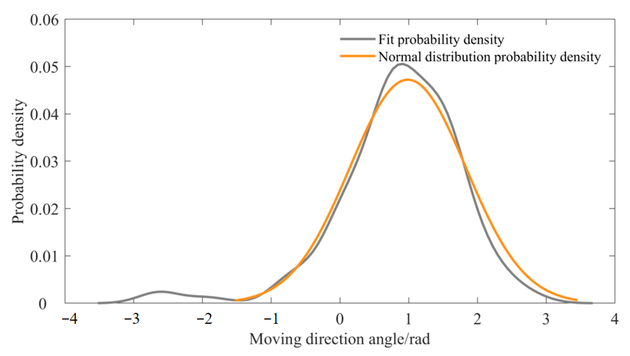
The moving direction angle, moving speed and central air pressure difference at the moment of typhoon landfall together constitute a set of typhoon landfall parameters, which can be implemented to simulate the operation of the typhoon after landfall. The typhoon path is dominated by large-scale circulation, and the moving direction angle fluctuations can be regarded as the superposition of multiple random factors, which conforms to the central limit theorem and leads to a normal distribution. The central moving speed is affected by the product effect of multiple factors. For example, an increase in pressure gradient may exponentially accelerate typhoons, which conforms to the characteristics of a lognormal distribution where the product of multiple random variables is logarithmically normal. The pressure difference reflects the strength of a typhoon, and its maximum value is limited by ocean heat capacity, wind shear, etc., which conforms to the threshold effect of Weibull distribution. The process of typhoon intensification is similar to a “chain reaction”, and Weibull’s shape parameters can flexibly fit the different stages of typhoon development.
As shown in Equations (1)–(3), the corresponding parameters were simulated using normal distribution, lognormal distribution and Weibull distribution, respectively [
19].
The moving direction angle at the moment of typhoon landfall
obeys the normal distribution with a probability density function:
where
is the mean of
in the normal distribution.
is the standard deviation of the normal distribution.
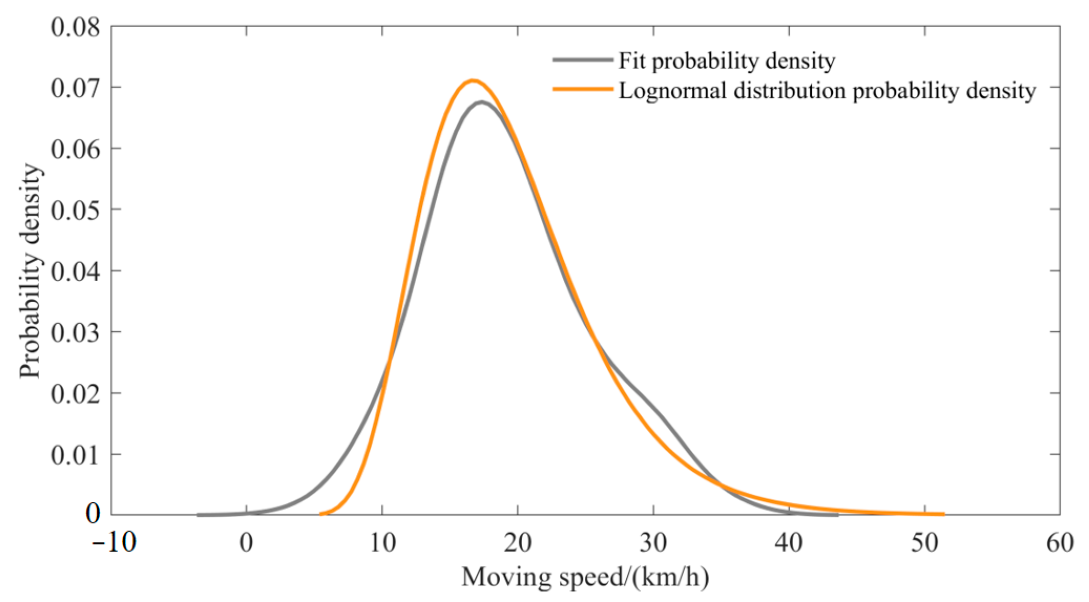
The central moving speed at the moment of typhoon landfall
obeys the lognormal distribution with a probability density function:
where
is the mean of
in the lognormal distribution.
is the standard deviation of the lognormal distribution.
The central air pressure difference at the moment of typhoon landfall
obeys the Weibull distribution with a probability density function:
where
is the scale parameter of the Weibull distribution.
is the shape parameter of the Weibull distribution.
Based on the probability density function of each typhoon landfall parameter, several sets of typhoon landfall parameters can be generated by Monte Carlo method [
20]. Subsequently, K-means clustering based on the contour coefficient method is used to obtain typical typhoon landfall parameters [
21].
2.2. Uncertainty in Typhoon Trajectory Modelling
Existing studies mostly regard the typhoon motion as a straight-line moving path, which has the problem of low accuracy and also affects the calculation accuracy of the subsequent typhoon disaster-triggering factors [
22,
23]. Therefore, this paper adopts the storm track model to achieve typhoon disaster path derivation, which can achieve real-time simulation of typhoon movement direction and movement speed, and better consider the uncertainty of the typhoon trajectory, so as to achieve accurate modelling of disasters [
24].
Based on the storm track model, the change in the natural logarithmic value of the typhoon center’s speed of movement and the change in the angle of direction of movement for the next moment can be determined from the typhoon center’s position, speed of movement and angle of direction of movement at the historical moment, as shown in the following equation [
24]:
where
are the storm track model parameter.
and
are the longitude and latitude of the typhoon center at time
, respectively.
is the moving speed of the typhoon center at time
.
and
are the moving direction angle of the typhoon center at time
and time
, respectively.
Therefore, the speed and direction of movement of the typhoon center at time
are calculated as follows:
2.3. Uncertainty in the Intensity of Disaster-Triggering Factors
2.3.1. Typhoon Wind Field Simulation
In this paper, the Batts model is used to simulate the typhoon wind field [
25]. Due to the different geographical locations of DNs components and the changing location of the typhoon wind field, the intensity of the disaster-triggering factor to which the components are subjected is time-varying. The wind speed disaster-triggering factor is calculated as shown in the following equation:
where
and
are the wind speed inside and outside the maximum wind radius, respectively.
is the maximum wind radius.
is the maximum wind speed;
is the distance from the typhoon center to the component location.
is the attenuation parameter.
The maximum wind radius and maximum wind speed are modelled as shown in the following equation:
where
is the central air pressure difference at time
.
is the central air pressure difference at the time of typhoon landfall.
is the angle between the horizontal direction and the direction of typhoon travel.
is the typhoon cyclone gradient wind speed.
is the overall typhoon movement speed. K is the empirical coefficient, which is taken to be 6.72.
is the angular speed of Earth’s rotation, which is taken to be 0.004178°/s.
is the geographical latitude.
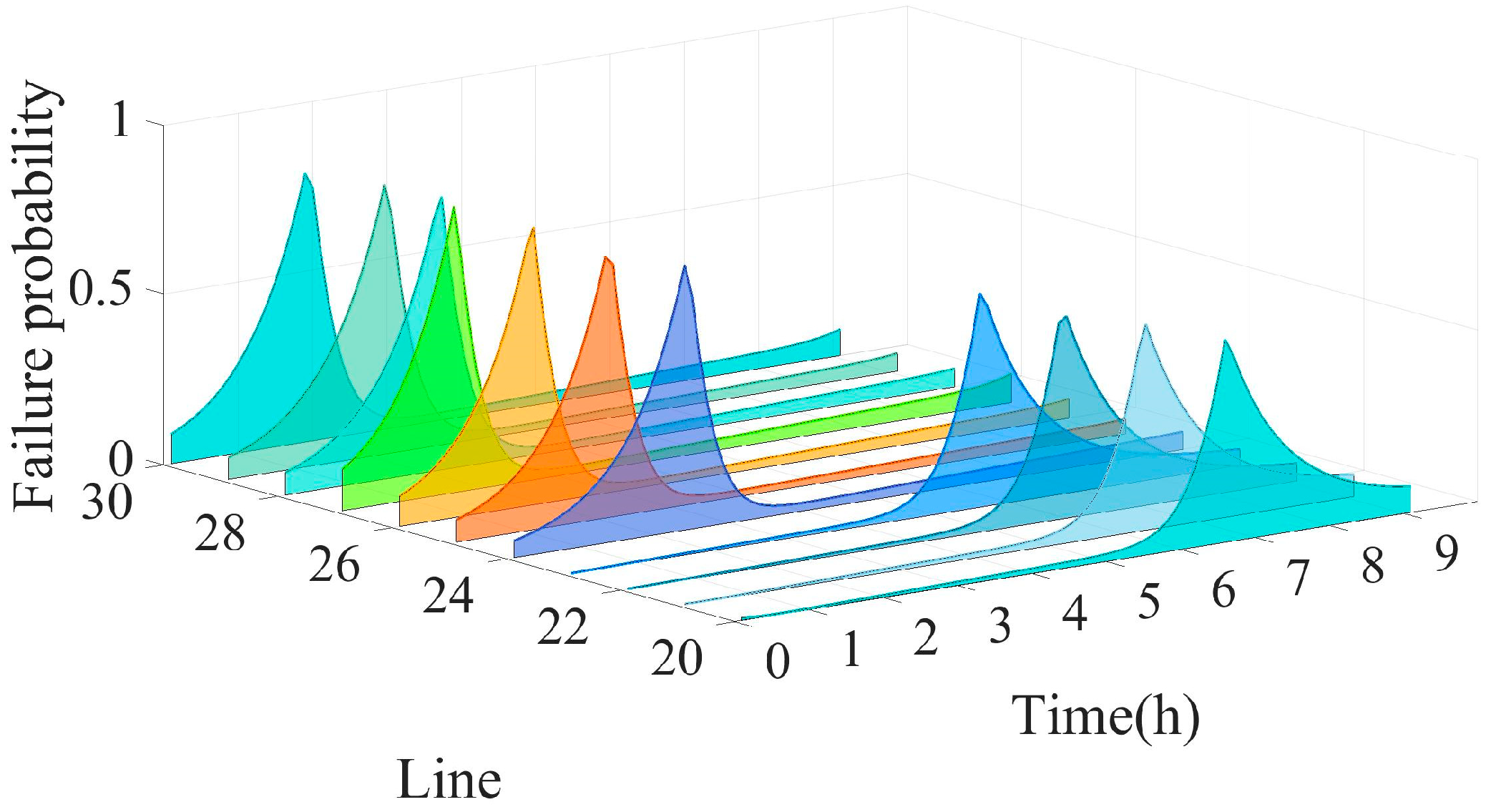
2.3.2. Component Failure Probability Model
When a typhoon strikes, strong wind and heavy rain cause great strain on the lines and towers of DNs, causing failure events such as broken lines and collapsed or tilted towers [
26]. Therefore, the failure probability of lines and towers caused by the disaster-triggering factors is considered.
- (1)
Tower Failure Probability
Typhoon wind damage mainly affects towers, and its failure rate can be quantified by the bending moment
on the towers caused by the wind load
on the lines and
on the towers [
26]:
where
is the wind pressure inhomogeneity coefficient.
is the wind pressure height variation coefficient.
is the line body shape coefficient.
is the outer diameter of the line.
is the distance from the tower.
is the angle between the line and the wind direction.
is the wind vibration coefficient.
is the wind load body shape coefficient.
is the projected area of the tower.
is the height of the tower.
is the distance from the root of the pole to the cross-burden.
is the additional bending moment coefficient.
and
are the diameters at the top and at the root of the pole, respectively.
The tower flexural strength approximately follows a normal distribution with a failure probability:
where
,
and
are the maximum bending moment, average bending strength and standard deviation that the tower can withstand, respectively.
- (2)
Line Failure Probability
The impact of typhoon rainfall on DNs is mainly concentrated on the power lines. The horizontal pressure
and vertical pressure
due to raindrops on the lines are calculated as follows [
26]:
where
is the rain density.
is the normalized curve integral value.
is the raindrop spectrum.
and
are the horizontal and vertical wind speed of the typhoon, respectively.
is the diameter of the raindrops.
is the velocity ratio.
is the elevation of the line.
is the correction coefficient.
is the rainfall intensity.
Line failure probability is quantified by loading under the influence of rainfall:
where
,
and
are the horizontal, vertical and total loads on the line from the rainstorm, respectively.
The line tensile strength approximately follows a normal distribution with a failure probability:
where
is the line failure probability.
is the maximum elastic limit of the line.
and
are the mean and standard deviation of the maximum elastic limit of the line, respectively.
- (3)
Integrated Failure Probability
Compared with the wind field, the scale of a single line of DNs is smaller, so the tower and line within the range of the bus can be regarded as a set of series components. Therefore, the integrated failure probability of DNs under combined wind and rain disasters is shown in the following equation [
27]:
where
is the integrated failure probability.
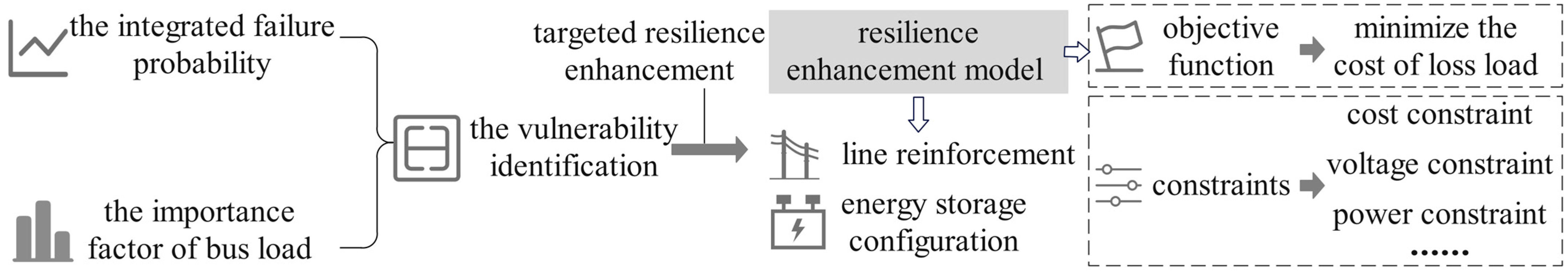
3. Vulnerability-Based Resilience Enhancement
Based on the integrated failure probability and the importance factor of bus load, vulnerability identification is achieved, and targeted resilience enhancement is carried out for vulnerabilities. The model is demonstrated in
Figure 1.
3.1. Vulnerability Identification
Vulnerable assessments can identify vulnerability in DNs, allowing resilience measures to be targeted in subsequent enhancement. This improves the effectiveness and economy of enhancement.
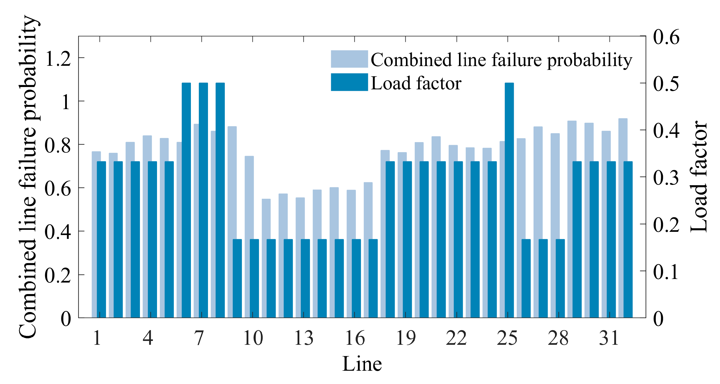
Based on the integrated failure probability and the importance factor of bus load under the influence of typhoon disaster, the integrated vulnerability index is defined as shown in the following equation:
where
is the integrated vulnerability indicator.
and
are the weighting factor.
is the importance factor of the bus load.
This paper adopts the hierarchical analysis method to determine the weight of each indicator [
28]. Firstly, based on the relative importance of each element to the upper level of decision-making, all the constituent elements of each level are compared two by two to form a judgement matrix. Then, the maximum eigenvalue solved according to the judgement matrix is checked for consistency. Finally, the vector of weights of each indicator is calculated. The steps are as follows:
- (1)
Creating the judgement matrix
Set
indicator be
. Adopt the 1–9 scale method shown in
Table 1 to obtain the scoring information of each indicator according to the preset scale from the experts, compare the scores of each feature quantity in the indicator layer two by two, and construct the judgement matrix [
28]:
- (2)
Consistency check
The construction of judgement matrices using the hierarchical analysis method depends mainly on the personal experience of the decision maker, and different decision makers construct different judgement matrices, which ultimately leads to the arbitrariness of the results, so the results must be checked for consistency. The consistency indicator is shown in the following equation:
where
and
are the order and maximum eigenvalue of the judgement matrix, respectively.
The consistency ratio indicator is:
where
is the stochastic consistency indicator.
The smaller the calculated is, the better the consistency of the judgement matrix. The feature vectors that pass the calibration are the weight vectors, otherwise the judgement matrix needs to be reconstructed.
- (3)
Calculation of weights
Normalize each column element of the judgement matrix:
The judgement matrix is summed by rows to obtain the initial subjective weight
:
Normalized again to obtain the final subjective weight matrix:
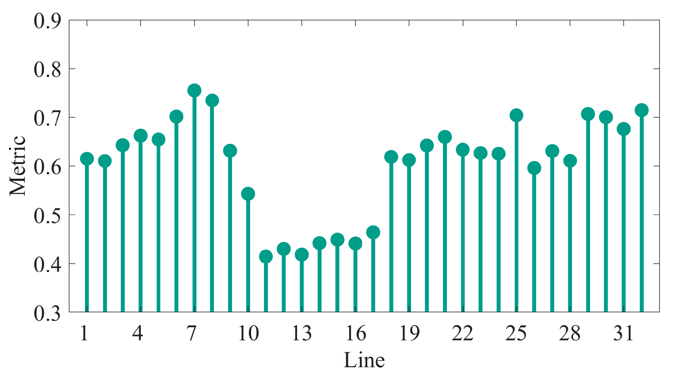
Compared with the quantification of a single indicator, the integrated vulnerability calculation method in this paper can more accurately identify the vulnerability of the system. When the integrated failure probability is large but the load importance is average, these lines are prone to be attacked and generate load loss when the typhoon passes through, so they should be analyzed for vulnerability. At the same time, for those links that have low failure probability but high load importance, although the probability of failure is low, once it occurs, it will cause great loss to the system, so it should be paid enough attention to it as well. After determining the calculation weights of each indicator, the integrated vulnerability indicator corresponding to each line can be calculated, and the higher the value of this indicator, the more likely it is to suffer load loss in a typhoon scenario. Therefore, the top 12 lines with high vulnerability indexes are selected as the vulnerability of DNs, for which line reinforcement and energy storage configuration measures are taken during the typhoon transit to reduce the load loss after the typhoon attack.
3.2. Resilience Index
In order to quantify the resilience of DNs under extreme typhoon weather, this paper takes the system lost load cost as the resilience indicator, as shown in the following equation [
29]. The larger the value of lost load cost is, the worse the system resilience is, and the smaller the value is, the smaller the load loss of DNs under typhoon disaster is, i.e., the better the system resilience performance is.
where
is the cost of lost load in DNs.
is the cost per unit of lost load.
is the load weighting factor of bus
.
is the amount of lost load at bus
.
3.3. Vulnerability-Based Resilience Enhancement Model
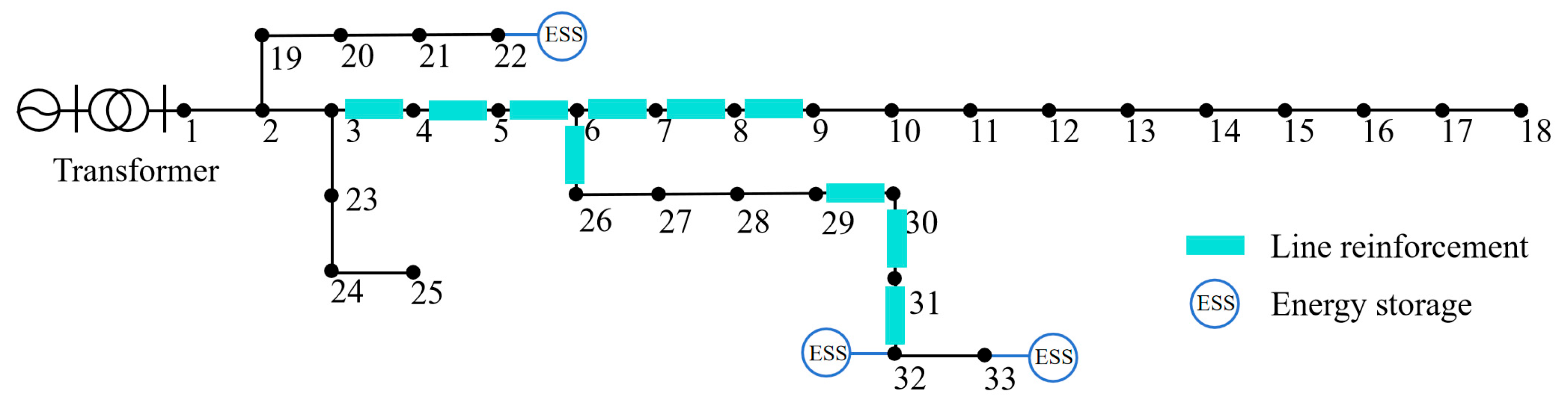
Line reinforcement improves the physical resilience of the system, and energy storage configuration enables emergency response in disasters [
30]. Based on the two resilience enhancement strategies, the location and capacity of the reinforced lines and energy storage configuration are determined with the aim of maximizing the resilience enhancement of the system during the emergency response to the disaster at a limited investment cost. The optimal investment cost is determined by the resilience enhancement benefit index. The index quantifies the resilience enhancement effect under the unit investment cost, and takes into account the system resilience enhancement effect and economy, as shown in the following equation:
where
is the resilience enhancement effect.
is the line reinforcement cost.
is the energy storage cost.
Line reinforcement cost is [
9]:
where
is the cost of line reinforcement per unit length.
is the length of line
.
indicates whether line
is reinforced or not.
is the set of lines.
The cost of energy storage
consists of the cost of the storage equipment
, the cost of the storage site
, and the total O&M cost
[
9]:
where
and
are energy storage unit power and capacity cost coefficients, respectively.
is the energy storage site cost coefficient.
is the energy storage annual O&M cost coefficient.
is the energy storage capital recovery coefficient.
and
are the rated power and capacity of the energy storage installed at bus
, respectively.
is a 0–1 variable that indicates whether or not to install the energy storage at bus
, and takes 1 if it is installed, and vice versa.
is the set of buses.
The objective function is to minimize the cost of system loss of load, as demonstrated in the following equation, aiming to minimize the resilience metrics proposed in this paper, i.e., to maximize the system resilience performance, by adopting the resilience enhancement strategy using line reinforcement and energy storage configuration.
where
and
are the inequality constraints and equation constraints, respectively, specified as [
9]:
- (1)
Investment budget constraint
- (2)
Active and reactive power balance constraints
where
,
and
are different buses.
and
are the set of parent and child buses of bus
, respectively.
and
are the active and reactive power flowing on line
at time
, respectively.
and
are the active and reactive power injected into DNs by the transformer at time
, respectively.
is the storage discharge power at bus
at time
.
is the reactive power output of the storage system at bus
at time
, assuming that there is sufficient reactive power compensation capacity for the storage.
and
are the active and reactive loads at bus
at time
in the normal case, respectively.
is the reactive power load lost at bus
at time
.
- (3)
Voltage relaxation constraints
where
is the voltage value at bus
at time
.
is the rated voltage value.
and
are the resistance and reactance values of line
, respectively.
is a large constant.
is the state of line
at time
.
- (4)
Line current constraints
where
is the transmission capacity of line
.
- (5)
Loss load constraints
- (6)
Bus power injection power constraints
where
and
are the maximum active and reactive power injections from the power supply at bus
, respectively.
- (7)
Bus voltage constraint
where
and
are the upper and lower voltage limits at bus
, respectively.
- (8)
Buses are allowed to install energy storage ratings and capacity constraints
where
and
are the maximum rated power and capacity of the energy storage allowed to be installed at bus
, respectively.
- (9)
Constraint on the amount of energy storage allowed to be installed in DNs
where
is the maximum number of energy storage installations permitted for DNs.
- (10)
Energy storage discharge power constraint
- (11)
Energy storage charge state constraint
where
and
are the minimum and maximum charge state values of the stored energy, respectively.
is the residual power from energy storage at bus
at time
.
- (12)
Energy storage power balance constraint
where
is the discharge efficiency for energy storage.
- (13)
Energy storage initial power state constraint
where
is the electricity value of energy storage at bus
at time
.
5. Conclusions
To address DN vulnerability under extreme weather, a typhoon-specific resilience enhancement method is proposed that incorporates multiple sources of typhoon uncertainty. First, typhoon impacts are simulated and network vulnerabilities are identified. Then, an optimization model is established to maximize system resilience. The effectiveness of the method proposed in this paper is verified, and the following conclusions are drawn:
- (1)
A disaster simulation method based on multiple uncertainties has been achieved. This solves the problem of poor accuracy in disaster simulation due to random parameters and linear trajectory in traditional methods, and improves the accuracy of the component failure probability model.
- (2)
A method for identifying vulnerability in DNs is proposed. This takes into account the impact of disasters and the stability of the power supply, providing a basis for the subsequent development of anti-disaster measures and avoiding the waste of resources associated with the traditional method.
- (3)
A resilience enhancement model based on line reinforcement and energy storage configuration is established. Compared to Case 1, the proposed method can reduce the system’s load loss by 5.112 million. And compared to Case 2, the proposed method reduces the load loss cost by up to 0.2459 million with a cost difference of 0.0595 million, which solves the problems of uneven resource allocation and poor economy of a single resilience enhancement strategy.
In this paper, only the pre-disaster resilience enhancement for typhoons is considered, and in the future, a variety of resilience resources can be combined for post-disaster scheduling to further improve the resilience of the distribution network under extreme typhoon disasters.


