Intertemporal Allocation of Recycling for Long-Lived Materials from Energy Infrastructure

Abstract

Energy conversion and infrastructure facilities consist of large amounts of metal and have lifetimes of several decades. When recycling metals, the methods of allocation play a decisive role in evaluating how primary and secondary materials, as well as the products that are produced with them, are to be evaluated ecologically. So-called credits for recycling are the subject of a particularly controversial discussion. This article shows that the current practice of giving credits for long-lasting products leads to a significant distortion of the actual emissions. Using the examples of steel, aluminum, and copper, prospective LCA data is used to show how the carbon footprint actually behaves. When credits are applied, the time dependency of emissions must be taken into account; otherwise, burden shifting into the future occurs, which can hardly be considered sustainable. The increase compared to the conventional time-independent practice lies, depending on the metal, at 70 to 300%. It is recommended that the cutoff approach be used conservatively when allocating recycling cascades in order to optimize environmental impact and avoid greenwashing.

1. Introduction

In the world of life cycle assessments (LCA) and product carbon footprints (PCF), the recycling of materials such as metals is understood as a joint process, i.e., as the coupled occurrence of two uses. This means that the same metal is used for several products in succession. Generally, this multi-use cascade consists of an initial product system that uses the primary material directly after its extraction, as well as one or more subsequent product systems that reuse the recycled material, i.e., secondary use. In the following, we will refer to primary material and the primary product system as well as secondary or recycled material and the secondary product system.

In most cases, the natural resource input and environmental burden of primary extraction are greater than those of material recycling and its reuse in the secondary product system. This results in a certain conflict in evaluating the two life cycle phases because the secondary material would not exist without the primary extraction. Does it therefore have to bear a share of the burden of the primary extraction? This leads to the question as to whether natural resource input and environmental burden between the two systems should be considered separately or whether they should be considered in total and allocated to the two systems according to a certain distribution key. In LCA technical language, this step is called allocation [1]. However, it is also often referred to as partitioning [2]. Depending on how the allocation is made, the primary and secondary systems can be favored or burdened very differently.

The question of the allocation of joint processes, especially in the case of recycling, has been the subject of intensive and controversial discussion since the LCA method was first introduced (e.g., [3,4,5]). Which approach is preferable depends on the epistemological interest [6,7], on cultural preferences [8], or on the choice of method [9,10]. We refer to the works by Schrijvers et al. [11], Frischknecht [12], or Guinée et al. [13] for their excellent summaries of the extensive publications that have appeared on this topic in recent years.

In a so-called closed-loop system, the secondary material is reused directly in the same product system, thereby replacing primary material. There is broad consensus on how to calculate this, namely with a kind of net input. This is also explicitly mentioned in ISO 14044 (Chapter 4.3.4.3.3) [1].

However, the treatment of an open-loop system, i.e., one in which the secondary material is generally used in a different product system, is controversial. Fava et al. [3] initially proposed a 50–50 split between the primary and secondary product systems. The greatest contrast exists between a recycled-content approach, which is also often referred to as a cutoff approach, and an avoided-burden or end-of-life approach (EoL), where the primary system receives a credit for the secondary material [14]. In addition, there is the so-called Circular Footprint Formula (CFF), or EU approach [15], as well as offsetting based on the number of uses in the cascade [16].

Our project, funded by the German Federal Ministry for Economic Affairs and Energy, focuses on products from the energy industry and their recycling. Power plants, wind turbines, PV systems, and the supporting technology for electricity distribution have product lifetimes of several decades. What happens to the materials, which are mostly metals, after the facilities have reached the end of their use phase? How are they recycled, and under what conditions?

In addition, there is the question of how allocations between primary and secondary use can be made over such a long period of time. The consideration of time in LCA and PCF is a recurring topic of expert discussion (e.g., [17,18,19]), but to date, there is no clear procedure, and most analyses are carried out independently of time, not least because, in most cases, no prospective data have been available for the inventories and the impact assessment. However, allocation formulas that divide the environmental impacts of a material between its first use and subsequent uses in a product system usually contain the emissions associated with primary production, recycling activities, and disposal. For primary production of metals, global plans for decarbonization will likely lead to a significant decrease in emission factors for some metals over the upcoming decades [20]. Hence, for long-lasting goods, the incorporation of temporal considerations in LCA has the potential to yield outcomes that diverge significantly from those of static calculations.

When dealing with recycling allocation, it was usually tacitly assumed that the products in question are short-lived and that market and environmental conditions do not change. This means that there is still demand for primary and secondary materials and that emissions have not changed significantly. However, the allocation problems that arise with long-lasting products have been addressed [8,21,22] suggested that credits for later recycling should not be given for long-lasting products, such as buildings, because this would significantly distort the real and time-dependent energy and material flows. Accordingly, in the European standard EN 15804 [23] for EPDs, a credit for recycling is not included in the calculation but is simply given separately as information.

In practice, the influence of time on a life cycle inventory has rarely been considered since the data used to calculate LCA usually describe the status quo of the technosphere in static terms (Ecoinvent, GaBi). With the development of the prospective “Premise” tool based on Ecoinvent, time-dependent data are now also available. These were partially updated as part of the Circular Energy Transition project, allowing the influence of time on allocation during recycling to be examined using case studies. We suspect that the LCA or PCF of the product systems change significantly when time-dependent allocations are made. In this article, the allocation approaches described above are considered for some metals, assuming that there is a longtime lag of several years or decades between the primary product system and the secondary product system. The calculation of credits in the closed-loop case is also re-examined since the conditions for raw material extraction and recycling may change over time.

2. Methods and Data

2.1. Selected Allocation Approaches

Various authors analyze the recycling cascade by formulae, taking different aspects into account [11,12,15]. The EU [15], for example, uses the CFF to distinguish between emissions from production and recycling at different points in the cascade and marks them with an asterisk. This makes it possible to differentiate to a certain extent over time. It also uses quality factors Q to account for the loss of quality of the recycled materials. However, Frischknecht [12], for example, does not use such quality factors. In addition, the EU [15] introduces a regulatory parameter A that is intended to reflect market conditions and thus allow control over whether the goal should be to increase the recycled content in products or to design products for recycling (see below).

In the following, it is assumed that the quality of the recycled material does not change, which is actually the case for some metals, e.g., copper. Furthermore, market influences are ignored, i.e., the question of whether there is a market for buying and supplying recycled material.

In this article, each allocation approach is described as a simplified system comprised of the steps of the material’s primary production, recycling, and disposal. Transportation, collection processes, and so forth are implicitly included. Other emissions that arise from the manufacture and use of the product are not taken into account. These must, of course, be correctly modeled as a function of time if the product in question has a long lifespan, e.g., if the product requires electricity during its use phase. However, this is outside the scope of this study.

As a representative example of the natural resource input and environmental burden, only a generalized emission E is considered here, without loss of generality, which arises from the use of the material in the product system. We use a notation based on Frischkecht (p. 88, [12]).

Parameter	Description
E	Emissions from production, recycling, and disposal of the material
e	Specific emissions (i.e., per quantity)
m	Quantity of the material
Subscript P, R, D	Represents production, recycling, and disposal
Superscript o, *	Represents previous time period and subsequent time period

2.1.1. Closed-Loop Approach

There is widespread agreement in the LCA community that the closed-loop case is easy to handle. The ISO 14044 standard makes a similar point. This case assumes that the recycled material remains directly in the same product system and thus reduces the use of primary material and the corresponding emissions (e.g., in [13], 91f.). This makes sense for products with a short lifespan, where the processes and markets involved do not change. The formula for the emissions E associated with the material input for the product is then as follows:

E = (m_P − m*_R) · e_P + m*_R · e_R + m*_D · e_D

(1)

where m_P is the amount of primary material entering the product system, m*_R is the amount recycled after the use phase and replacing primary material, and m*_D is the amount not recycled and requiring disposal.

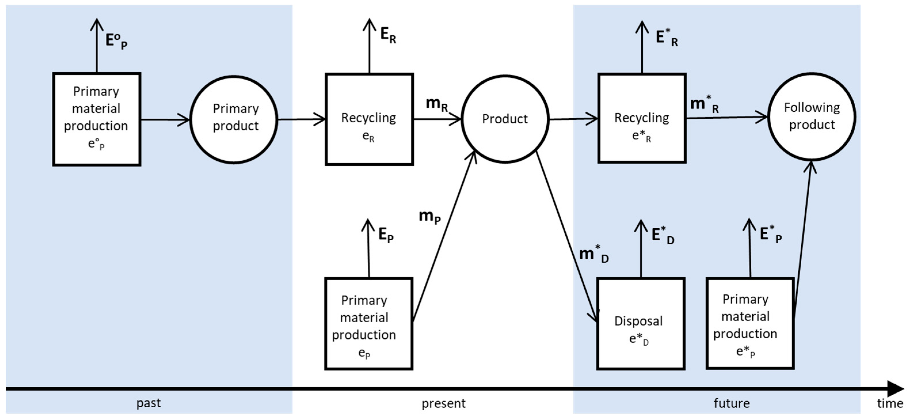
If the system is applied to a product with a long lifespan, the recycled material is only available after the product’s use phase. But in the conventional case according to Formula (1), it is offset against the material at an earlier point in time (Figure 1, left side). In simple terms, the diagram shows a material return flow against the direction of time (red arrow). This gives the false impression that the primary material requirement at the earlier point in time is lower due to recycling. However, this is factually incorrect. Only the primary material requirement produced at the same time as the recycled material, i.e., in the future, can be saved.

The closed-loop approach can also be used when the secondary material has inherently the same material properties as the primary material but is used in a different product system ([1], Chapter 4.3.4.3.3). This allows the system to be correctly mapped over time (Figure 1, right), whereby the subsequent product can be either the same or a different one. The only thing that matters is that the material has the same inherent properties. However, the production, recycling, and disposal processes may change over time, causing different specific emissions. Such changes are highly likely for greenhouse gas (GHG) emissions due to the planned global decarbonization of industry over the next few decades.

This also yields the formula for correctly calculating the emissions E associated with the material input for the product:

E = m_P · e_P − m*_R · e*_P + m*_R · e*_R + m*_D · e*_D

(2)

2.1.2. Recycled-Content or Cutoff Approach

When using recycled-content approach, only the emissions from the production of the primary material that has been incorporated into the product are allocated to the product. The same applies to the secondary material contained in the product. Only the recycling of this secondary material is taken into account. In addition, the disposal of the wasted material that leaves the product is also allocated to the product. If a product contains only recycled material, no emissions from primary production are allocated to it. This is often referred to as a cutoff approach because the primary and secondary systems are effectively separated and no offsetting takes place between the two. According to Atherton [14], this provides a metric that describes the origin of the material and provides a measure of waste diversion. The approach is based on a waste management perspective, where the general aim is to promote a market for recycled materials.

In the case of long-lasting products, it must be taken into account that the recycling and disposal of the used material will take place in the future (Figure 2). Therefore, future conditions must be assumed for the emissions. However, it can be assumed that the use of primary and recycled materials will take place during the same period in which the product is manufactured.

The emissions of the material used in a product are calculated from the sum of the emissions from the production of the primary material used, the emissions from the recycling of the secondary material used, and the emissions from the disposal of the material remaining at the end of the use phase.

E = m_P · e_P + m_R · e_R + m*_D · e*_D

(3)

2.1.3. Avoided Burden or End-of-Life Approach

The end-of-life approach considers the fate of products after their use phase and the resultant material output flows. The recycled material replaces a certain amount of primary material, which does not have to be extracted, thus reducing natural resource input and environmental burden. This is why this approach is often referred to as avoided burden or substitution. The reduction in natural resource input and environmental burden is credited to the primary material or the product that is created from it. Atherton [14] argues that a designer should then focus on optimizing product recovery and recyclability of materials, i.e., a design-for-recycling concept. According to Atherton [14], the international metals industry favors the end-of-life approach over the recycled-content approach.

The emissions are calculated from the total quantity of material (primary and secondary) and the specific emissions from the production of the primary material [12]. Furthermore, the emissions from recycling of the recycled quantity and the emissions from disposal of the disposed quantity are taken into account. The emissions potentially avoided by the recycled quantity are subtracted from the production emissions of the primary material. If we neglect the changes in the emission factors over time, we get

E = m_P · e_P + m_R · e_P + m*_R · e_R − m*_R · e_P + m*_D · e_D

(4)

If we refer to Figure 2 and the considerations for the closed-loop case, it becomes clear that for long-lasting products, a distinction must also be made according to the time of the emissions. Again, the avoided production of primary material (which is equal to m*_R) can only be credited in the future with the term –m*_R · e*_P. In the present, on the other hand, the full amount m_p must be provided under today’s production and emission conditions.

E = m_P · e_P + m_R · e_P + m*_R · e*_R − m*_R · e*_P + m*_D · e*_D

(5)

In this case, the primary production of the material, which is included in the product as a recycled quantity, must be taken into account. This is what the term + m_R · e_P stands for. For this, the emission factor of the current period e_p is used. The reason is that this term must balance with the credit granted one step earlier in the cascade. Through the credit, a certain amount of emissions E_credit is shifted from the past into the future. However, the real emissions E_past occurred in the previous period. If e_P < e^o_P, then a δE in the overall balance disappears as a result of the credit.

E_past = m_R · e^o_P

(6)

E_credit = m_R · e_P

(7)

δE = m_P · (e^o_P − e_P)

(8)

Further, if we assume that metals do not have to be explicitly disposed of after the use phase, but that a certain proportion of them dissipate, then the disposal term can be neglected. Nevertheless, for thermodynamic reasons, m*_R < m_P + m_R applies, and if we assume that only primary material is used, m*_R < m_P. Equation (4) is then simplified to

E = m_P · e_P + m*_R · e*_R − m*_R · e*_P

(9)

As in the closed-loop case in Equation (2), a credit is given here for the emissions saved by the recycled material m*_R. This credit is the subject of much discussion and criticism (see Section 2.2).

2.1.4. Circular Footprint Formula (CFF) of EU

The EU’s CFF approach is complex and not easily understood. On the one hand, comprehension is complicated by factors that describe the quality of the secondary material m_R or m*_R in relation to the primary material m_P. Here, these quality factors are designated Q and Q*. On the other hand, the CFF includes factor A, which decides between a burden and a credit and is selected according to the market situation. It varies between 0.2 and 0.8 [24] but is usually 0.5 and thus corresponds to the established 50–50 approach of Fava et al. [3]. The original CFF does not explicitly address the time dependency of the emissions. But translated into the nomenclature used here, and into its time-dependent form, the emissions for the use of primary and secondary material would be as follows:

E = m_P · e_P + A · m_R · e_R + (1 − A) · m_R · e_P · Q + (1 − A) · m*_R · e*_R − (1 − A) · m*_R · e*_P · Q* + (1 − A) · m*_D · e*_D

(10)

If we set Q = Q* = 1 and A = 1, then

E = m_P · e_P + m_R · e_R

(11)

This is more or less the recycled-content or cutoff approach, as in Equation (3), where the emissions from the disposal of the material that is not recycled after the product life are missing here. In this case, A = 1, the product system is favored if as much recycled material as possible is used.

If we set A = 0 instead, the following applies:

E = m_P · e_P + m_R · e_P + m*_R · e*_R − m*_R · e*_P + m*_D · e*_D

(12)

Now, the time-dependent CFF coincides with the end-of-life approach of Equation (5). The product system is favored if as much recycled material as possible can be reused at its end of life. However, it should be noted that the EU’s CFF does not explicitly address the issue of time dependency, but it does take into account different emission factors—here according to the tag *.

The significance of the CFF approach lies in factor A, which can be used to switch seamlessly between the two methods, recycled-content and end-of-life. CFF also introduces the quality factors. Otherwise, it is a combination of the recycled-content and the end-of-life approaches.

2.2. Evaluating the Approaches

The widely used allocation approaches described in Section 2.1 can be converted into time-dependent approaches with the prospective LCA data that is now available. This is useful for long-lasting products. Nevertheless, the question remains as to which of these allocation approaches is “more correct”. This question can only be answered if more fundamental assumptions are made.

One of these assumptions concerns the decision-making situation. If an LCA or a PCF is created retrospectively for a product or from a bird’s eye or observer’s perspective as it were, the emissions (or natural resource input and environmental burden) are recorded over the entire life cycle of the product. Tillman [6] had already distinguished decision-making situations in “accounting LCAs” and “change-oriented LCAs,” which, in the technical discussion, ultimately led to the concepts of attributional and consequential LCA [25]: However, the time aspect was not considered at that time, as the focus was on the treatment of marginal datasets of processes.

However, if the issue is not an accounting LCA, but rather a decision that needs to be made in practice, e.g., whether and when to recycle material, how long a product should be used optimally, and so forth, then a different approach is called for. Then it is not about a fair distribution of emissions across products, from the bird’s eye view but about which emissions occur and to what extent can they still be influenced by the decision. Conversely, emissions that have already occurred in the past should be left out of this consideration. This would mean that emissions from primary production in previous use phases in the past should not be taken into account. Only present and future emissions should be considered. This would strongly support the cutoff approach, in which such offsetting is not intended anyway.

With regard to substitution or credits for the end-of-life approach, Frischknecht [12] advances a fundamental argument: a product that uses primary material today would be better off with a credit, as it would be credited with emission reductions that only occur in the distant future. Conversely, products in the future would be burdened with the emissions from primary production in the past. This would be burden shifting into the future and would contradict, according to Frischknecht, the principle of strong sustainability. De facto, however, the emissions or the extraction of raw materials would have already occurred today, and the emission reduction in the future would be hypothetical. One could say that this would be a form of greenwashing for today’s product. A low-emission product of the future, on the other hand, would have to live with an emissions burden from the past.

Other authors argue on a methodological level, according to which the substitution approach, in which a credit is given for avoided primary production, does not belong in the attributional LCA (e.g., [26,27,28,29,30]). If a credit is included at all, it should be in a consequential LCA. However, in this case, more stringent data requirements would have to be met because the processes and market developments would have to be modeled with marginal data.

Hofstetter’s [8] approach is very interesting in that he attributes the way we deal with future recycling to different cultural preferences. He distinguishes between individualists, hierarchists, and egalitarians (see Figure 3). “Individualists are risk-seeking and use an adaptive management style …. Egalitarians hold the opposite view … their worldview is based on the concept of an ephemeral (fragile) nature …. This requires a preventive management style …. Hierarchists show a high belief in expert judgements and the existence of evidence is their main criterion for deciding …. Hierarchists will also pay a great deal of attention to procedural aspects” ([8], p. 116f.).

According to Hofstetter, an individualist would argue that as long as there is a demand for the secondary material, one can easily attribute the environmental impacts of primary production to all subsequent secondary uses. Hierarchists would only accept this for products with short lifespans, for which market conditions can be foreseen, but not for the uncertain distant future. Egalitarianists, on the other hand, would argue that the primary material would have to be assigned the entire environmental burden because recycling in the future is rather uncertain. This shows that there is no correct or incorrect assessment here, but that it depends very much on cultural patterns or assumptions.

2.3. Data

The allocation approaches are exemplified on the basis of three product systems using the metals aluminum, copper, and steel. As an impact category, we have chosen climate change, i.e., we are looking at the carbon footprint, as significant changes in emission factors are expected in the coming years due to the shift in energy production toward more renewable energy sources. Figure 4 shows the carbon footprints over time. The carbon footprint (CF) quantifies the greenhouse gas emissions in kg CO₂ equivalents (CO_2e) per kg of metal produced. The data refer to German market conditions, but could be presented equally well for other countries. Instead of the CF, other environmental impacts could also be used. However, this is not crucial, as the focus here is on the general significance of the allocation approaches.

Cradle-to-gate CF of the primary and secondary production routes of the three metals were calculated for each five-year step between 2025 and 2050. The compilation of the data is explained in detail in the Supplementary Materials. For the background of the prospective models, the Ecoinvent 3.9.1 cutoff database was used after having been modified with so-called “Premise”. This tool [31] facilitates the harmonization of life cycle inventories (LCI) within the Ecoinvent database to align with the output data generated by integrated assessment models (IAMs). By doing so, it enables the development of LCI databases that reflect future policy scenarios. The scenario chosen for this study includes an optimistic forecast of societal, economic, and technological developments to limit global warming to a maximum temperature increase of 1.8 °C. The impact assessment was performed for the GWP₁₀₀ with characterization factors from the IPCC 2021. More detailed descriptions of data collection using the Premise tool can be found in Heidak et al. [32] in the same special issue of Energies.

For aluminum, emissions from primary production decrease dramatically over time. This is due to the decarbonization of electricity production, which plays a significant role in the electrolysis of primary aluminum. By contrast, emissions from the production of secondary aluminum are significantly lower but do not drop to zero even in 2050.

A similar picture emerges for copper, although the differences between primary and secondary production are not quite as drastic as for aluminum. The reduction in primary production is due to the greater electrification of mining. The increase in secondary copper in 2045 and 2050 is due to the return of low-quality scrap. Details can be found in the Supplementary Materials.

The situation is somewhat more complex for steel, as the conventional reduction of iron ore with coal is to be replaced in the future by reduction with natural gas or with green hydrogen. Natural gas would lead to a reduction in emissions compared to the classic converter process. But a significant reduction will only be achieved by using hydrogen, which will be increasingly produced with electricity from renewable sources over time. Even in 2050, the production of secondary steel would still be associated with lower emissions than primary production.

This finding that emissions will not be reduced to zero by 2050 may contradict the proclaimed ambitions to achieve carbon neutrality, as set out in German and European Community policy. On the one hand, this can be understood as a consequence of the globalization of economic processes. Not all regions of the world will be decarbonized by 2050. On the other hand, this finding may be due to the fact that not all sectors have been integrated into the Premise tool yet, nor have developments, such as efficiency increases or fuel mix changes, been fully integrated in some sectors [31]. So there will be a residual amount of emissions as an artefact.

3. Results

Various cases were calculated and compared using the equations described in Section 2.1 and the data described in Section 2.3. Waste disposal was neglected in the cases since it plays only a minor role for the three metals. We assume that metals from energy facilities are mostly recycled. However, if other materials (e.g., plastics) or consumer products are considered, disposal can make a certain contribution. The values in Figure 5, Figure 6, Figure 7 and Figure 8 always refer to the use of 1 kg of material, and the emissions are based on the product system into which the material is incorporated. In our cases, we assume that the product contains both primary and secondary materials. The amount of primary and secondary material used for the product is therefore taken into account, as is the amount of material that can be recycled back into secondary material after the product’s use phase.

We have assumed typical values for the recycled content (RC) in the product and for the end-of-life recycling rates (EoL RR) for all three metals: aluminum (RC = 40%, EoL RR = 70%), copper (RC = 60%, EoL RR = 85%), and steel (RC = 60%, EoL RR = 85%). These values may differ, especially in the future. This can be quickly recalculated using the values in the Supplementary Materials. However, this is not relevant for the influence of the time aspect on credits.

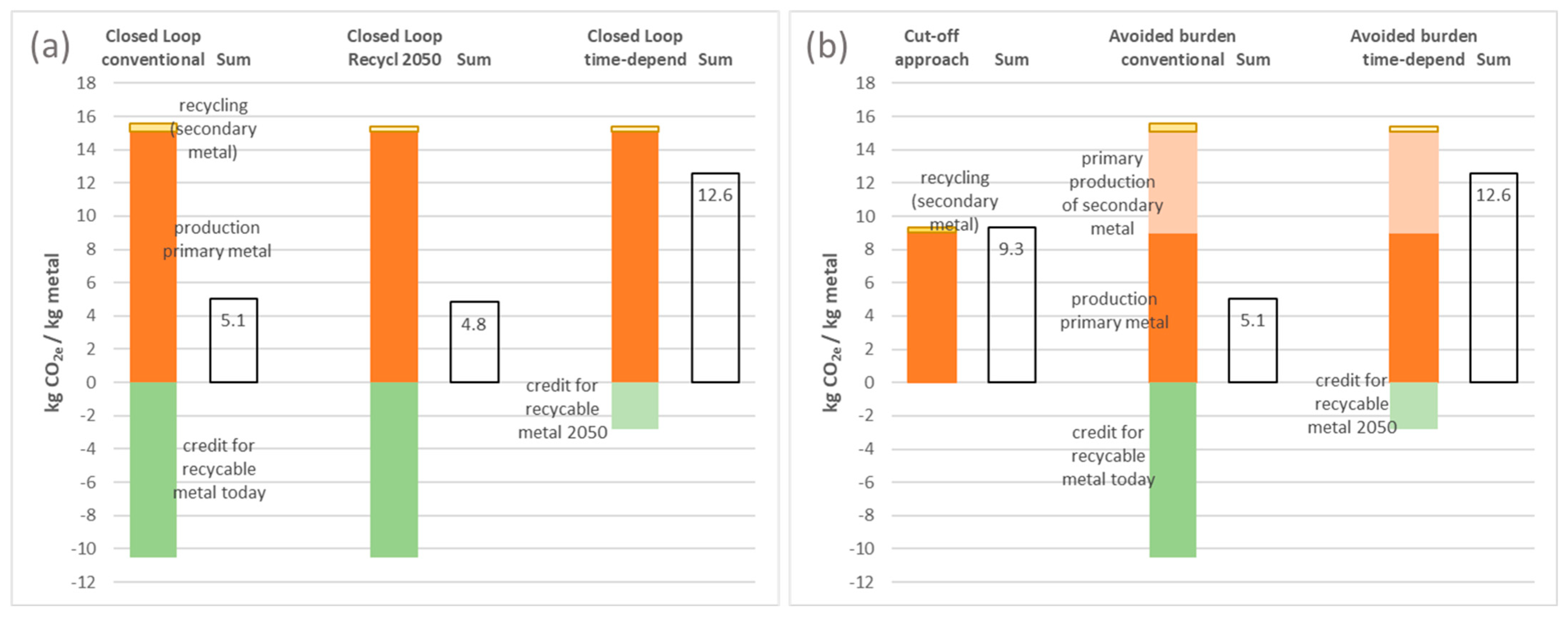
First, the closed-loop case was calculated for the three metals: aluminum, copper, and steel (Figure 5a, Figure 6a, Figure 7a and Figure 8a). The conventional case is time-independent, i.e., the emissions are all assumed to occur in the same time period. This corresponds to the usual approach when starting from time-independent LCA data, e.g., from the Ecoinvent database. In Figure 5a, for example, it can be seen that the carbon footprint for the use of 1 kg of aluminum in a product is then set at 5.1 kg CO_2e. While the actual primary production of the aluminum causes 15 kg CO_2e, 10.5 kg CO_2e is ultimately credited to it through the recycling of 0.7 kg of aluminum.

In the middle case in Figure 5a, it is assumed that recycling can only take place after the product’s use phase, i.e., in the future. Since it can be assumed that recycling will cause fewer emissions at that point, the overall carbon footprint is somewhat lower. If we now also consider that the secondary material will only be available in the future—in our case, in 2050—it can only then replace primary material and thus the corresponding emissions. Since it is also assumed here that the primary production of aluminum will be significantly lower than it is today due to decarbonization, the credit is lower (right case in Figure 5a). Consequently, the product system for the use of 1 kg of aluminum has to be burdened with 12.6 kg CO_2e.

Figure 5b shows the recycled content or cutoff case on the one hand. This is the simplest case because it only takes into account the emissions from the production of the primary material and the recycling of the secondary material in the present. Ideally, the emissions from disposal in the future would have to be taken into account, but they have been neglected here. This case can be said to reflect the real emissions in the present time period and also assumes that the process data are known.

The middle case in Figure 5b represents the EoL, or avoided burden case (i.e., the consideration of credits for the recycled material), as it is typically assessed independently of time. In this case, the emissions from primary production and recycling are offset by a relatively high credit of 10.5 kg CO_2e. This takes into account the primary production of the material that is already incorporated into the product as a secondary material. This production took place in the previous time period. It must be pointed out that if this time period is in the past, these emissions can no longer be prevented. In total, this approach would result in a burden of 5.1 kg CO_2e, which is almost half as high as the cutoff approach. This is also the reason for the popularity of the approach in business.

However, this approach only reduces the emissions of primary production on paper, namely through the credit that first takes place when the recycled material actually replaces primary material, in this case, in 2050. This is shown in the right-hand case in Figure 5b. The credit here is again significantly lower, so that the result in total is 12.6 kg CO_2e.

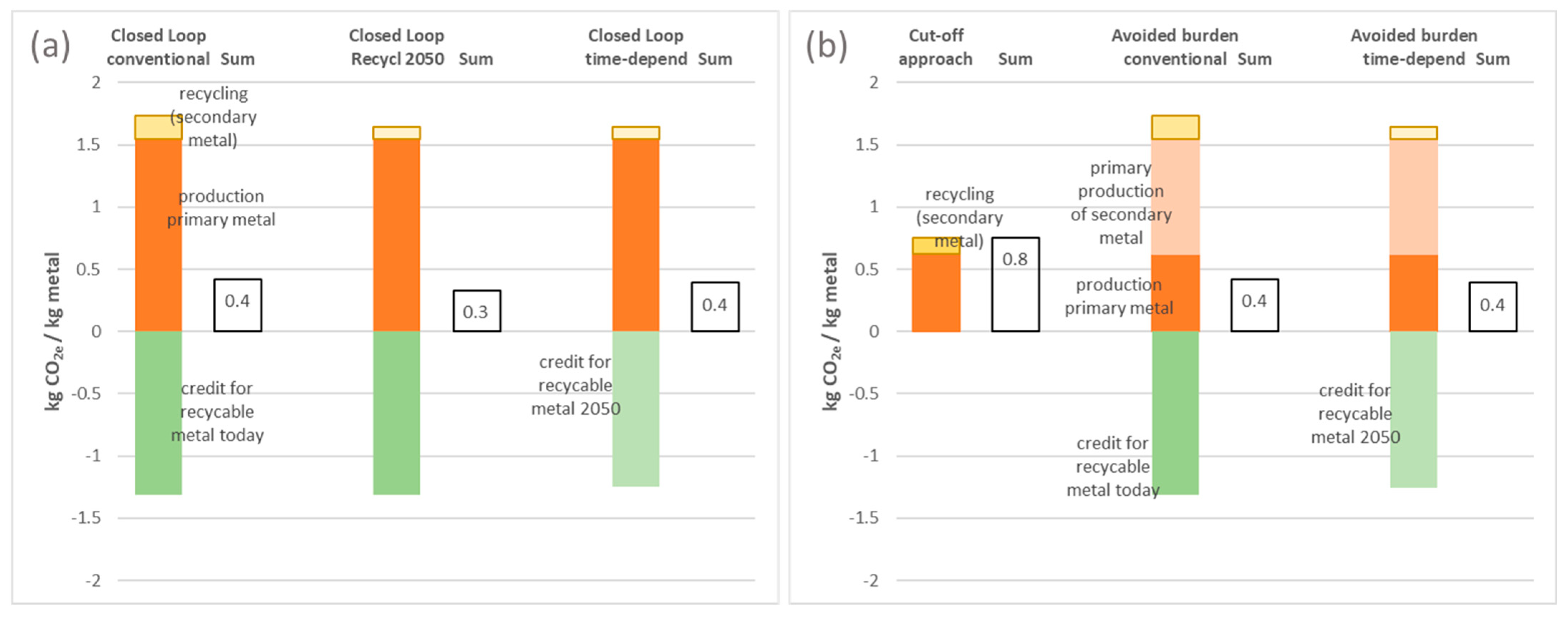
For aluminum, the difference in emissions between primary and secondary production is relatively large. This is mainly due to the decarbonization of electricity production. The differences are smaller for copper (Figure 6). But here, too, it is clear that considering the time for long-lasting products leads to a completely different picture. For copper, the time-dynamic consideration in the closed-loop case increases the PCF by more than half to 4.1 kg CO_2e per kg Cu. A similar value is obtained with the time-dynamic EoL approach. In contrast, the recycled-content approach yields 3.2 kg CO_2e per kg Cu. It works with data that is available for the present and does not need to be estimated.

The situation is somewhat different for steel and depends very much on the assumptions made in the manufacturing processes. Today, primary steel is produced in a blast furnace and an oxygen converter and, due to the chemical reduction, generates high CO₂ emissions. This process is not expected to see any major changes in the emission factors in the next few years. Figure 7 shows a conservative case with blast furnace and oxygen converter, even in 2050. However, there are significant improvements when the primary route is taken with other technologies, e.g., with reduction by natural gas or hydrogen. This would allow the oxygen converter with high emissions to be replaced by hydrogen with low emissions in the future, which leads to the usual credit problem (Figure 8).

4. Discussion

The calculations in this paper illustrate that time can have a significant influence on the PCF or the LCA of a product when allocations are made in recycling cascades. This opens the door to abuse, as the environmental impacts of a PCF or LCA can quickly be embellished, intentionally or unintentionally, when credits are allocated. This always occurs when long time periods are considered in the product life cycle, and the emission factors change significantly over time. From Equations (1) to (2) and (4) to (5), it can be seen that the time-independent and time-dependent analyses differ as follows:

Closed-loop recycling    ΔE = m*_R·(e_P − e*_P) − m*_R·(e_R − e*_R) − m*_D·(e_D − e*_D)

(13)

EoL approach          ΔE = − m_R · (e_P − e*_P) + m*_R · (e_P − e*_P) − m*_R · (e_R − e*_R) − m*_D · (e_D − e*_D)

(14)

It therefore depends largely on the change in the emission factors and the amount of secondary material. Particularly with regard to greenhouse gas emissions, significant dynamic changes must be expected in the coming years.

In the calculations in Section 3, the emissions from disposal were neglected, as for the metals considered, the recycling rate in waste is relatively high. Although losses occur during the recycling process (which have to be landfilled as, e.g., slag), these are rather low, and the GHG emissions from this will not change significantly in the future. The actual material losses tend to occur through dissipation along the entire life cycle. It cannot be ruled out that the metals will also be landfilled—trapped in products or other materials—but the values are difficult to quantify. Since this article is only intended to demonstrate the effect of the time dependency of the allocation on the PCF or the LCA, the simplification in the case studies seems appropriate. Generally, the equations are given correctly, i.e., with the disposal term.

The case studies discussed here are focused on GHG emissions, but they can also be generalized for other environmental burdens. The so-called life cycle inventory is in the foreground, namely with the emission factors of the GHGs. One problem must be pointed out here. As is common practice, the various GHGs were aggregated with the global warming potential (GWP) to CO₂ equivalents (CO_2e). This is a strong simplification for two reasons: on the one hand, dynamic analyses must take into account that the GWPs of different GHGs can change in relation to each other when the time scale is changed. This is due to the fact that, e.g., the lifetime of methane in the atmosphere is only 11.8 years, whereas that of nitrous gases is 109 years and that of some fluorinated compounds is several thousand years. On the other hand, it makes a difference to the climate impact whether a CO₂ emission occurs today or in 30 years. Strictly speaking, today’s emissions should not be offset against emissions in 30 years without scaling their climate impact accordingly. These aspects have already been pointed out [33,34,35,36]. In practice, this means that, in addition to the prospective data from the Premise database, which is provided at the inventory level, time-dependent impact systems are also required.

When primary material is substituted by secondary material and the associated emission credit is granted, it is implicitly assumed that there is a market for the secondary material and that substitution actually takes place. If, for example, demand for a material declines in the future, secondary material may no longer replace primary production or may do so to a lesser extent. Conversely, an increase in the supply of secondary material could lower the price and thus increase demand. Such rebound effects are neglected because they are difficult to predict. The market effects of material recycling allocation have been addressed in many studies (e.g., [37,38,39,40]). They also underlie the EU’s CFF approach, which the EU hopes will enable it to control the allocation and thus the burden on primary and secondary materials, depending on how elastically the markets react to the supply of secondary materials. These aspects have been neglected here. Such an approach assumes that a PCF or an LCA can have a significant influence on pricing and thus on the market for raw materials. In our opinion, this is not yet the case today. But if market effects are taken into account in the allocation, the allocation would also have to be done over time.

5. Conclusions

Energy systems such as wind turbines, PV systems, substations, and distribution grids have a life expectancy of up to several decades. They consist largely of metals, which can typically be recycled. This raises the question of how to calculate their PCF or LCA to adequately account for recycling.

In our considerations, we assumed that only those emissions that can be avoided in the present and in the future through appropriate action should be relevant to decision-makers. This excludes emissions from the past, which are, however, repeatedly included in various allocation approaches. In these cases, emissions that were emitted in the past to produce primary material are often also allocated to the secondary material or secondary product system.

This time aspect leads us to a dynamic allocation in which a distinction is made as to when the emissions were produced for the manufacture of the primary materials, the secondary materials, their previous primary materials, and their disposal. Since the technical conditions can change over time, care must be taken to ensure that credits are only given within the same time period, i.e., that there is no offsetting over time. Otherwise, there would be burden shifting into the future, with the result that today’s products would appear to have a lower PCF. This means that the current impact on climate change would be underestimated. Then, calculations regarding net-zero emissions could be greenwashing.

Case studies were calculated for the three metals: aluminum, copper, and steel. For this purpose, GHG emission factors from Premise tool were used that allow forecasts for primary and secondary extraction up to 2050. It was shown that taking time into account leads to significantly lower credits from substitution than time-independent calculations based only on common databases.

It is understandable that previous LCA and PCF practices have neglected the time aspect in allocation. This is due to a lack of reliable data for the future. The standards have not addressed this issue either. For example, the EU CFF explicitly requires credits for recycling. But time is not taken into account. ISO 14044 also does not consider the time aspect. Furthermore, ISO 14044 also contains a note in its Appendix D that substitution would be a way of implementing the normative requirement to avoid allocations by system expansion. It does not address whether substitution is permissible at all in the case of attributive LCA. At least Appendix D of ISO 14044 is only “informative” and does not constitute a normative recommendation. However, the situation regarding data availability has changed significantly. Therefore, the standards for LCA and PCF must take the time aspect into account when they are revised.

Analyses that allocate credits for recycling to long-lasting products give a false impression of low environmental impact. In our view, substitutions with secondary materials, and thus credits for long-lasting products, should be avoided. In the case of attributional LCA and PCF, the use of the recycled-content or cutoff approach makes sense. If credits are given in consequential LCA, then it should be demonstrated that there is no time lag in the calculation of emissions. That is, the substitution of primary materials should take place in the near future, not in the distant future.