Integration of Recent Prospective LCA Developments into Dynamic LCA of Circular Economy Strategies for Wind Turbines

Abstract

This study builds a bridge between the advancements from prospective life cycle assessments (pLCAs) and dynamic life cycle assessments (dLCAs) to improve the evaluation of circular economy (CE) strategies for long-lived products such as energy technologies. Based on a literature review of recent developments from pLCA and dLCA, an extended LCA methodology is proposed that provides guidance in the consideration and integration of technological and market dynamics across all major LCA steps of a dLCA, whose flows and impacts extend over a long period of time. This ensures a more accurate assessment of the impacts on global warming over time by explicitly incorporating temporal differentiation into goals and scopes, life cycle inventories, and interpretations. The methodology was applied to compare two CE measures for wind turbines: full repowering, including material recycling, and partial repowering. The analysis revealed that full repowering is the environmentally preferable option from the perspective of global warming potential, as the higher electricity output offsets the emissions associated with decommissioning and new construction. The findings were robust under various assumptions on future technological advancements, the underlying decarbonization scenario aligned with the Paris Agreement, and the application of discounting of future emissions. Ultimately, this work provides a practical yet adaptable approach for integrating future-oriented LCA methods into decision-making for more sustainable infrastructure and machinery.

1. Introduction

In order to effectively address the issue of climate change, it is imperative to facilitate a transition towards a more sustainable energy system, with a greater reliance on renewable energy sources. This in turn requires the construction of new energy plants and grids [1], requiring vast amounts of materials [2], including critical raw materials (as per the definition of the European Union [3]), such as copper and rare earth metals. Together with today’s energy infrastructure and the long lifetimes of the materials used in it [4], they will continue to serve as a large repository for a multitude of materials. For example, an analysis conducted by the German Environment Agency revealed the potential of a 368 kt of metal withdrawal between 2015 and 2040 from the German power plant infrastructure [5], including aluminum, stainless steel, zinc, and magnet materials. Given the current and projected demand for these materials and the amounts in use, it is prudent to consider the potential of a circular economy (CE). CE is known as an “economic system that replaces the ‘end-of-life’ concept with reducing, alternatively reusing, recycling, and recovering materials in production/distribution and consumption processes […] with the aim to accomplish sustainable development […]” [6]. To implement a CE, several strategies have been developed, which have often been summarized as the 10 R framework (Refuse, Rethink, Reduce, Reuse, Repair, Refurbish, Remanufacture, Repurpose, Recycle, and Recover) [7]. These R-strategies can be clustered into three overarching strategies, namely smarter product use and manufacturing, the extension of the lifespan of a product and its parts, and the useful application of materials, which mainly includes their recycling at the end of life. On the one hand, they are implemented to contribute to various objectives, such as enhancing the security of supply in countries that are dependent on raw material imports [8], reducing overall resource consumption, and decreasing environmental and social impacts [9]. On the other hand, it has been demonstrated that from an environmental perspective, CE strategies face limits when it comes to minimizing impacts, e.g., due to target material and chemical compound concentrations in products, and thus high efforts to recover materials [10,11]. Wind turbines represent an interesting case in this regard. In order to achieve the climate targets, the power generation capacity of onshore wind turbines is expected to at least double between 2018 and 2050 in Europe [2] and increase from 69 GW in 2024 to 160 GW in 2040 in Germany [12]. Two strategies are commonly used to counteract the shortage of space in German federal states and increase the installed capacity: use-phase-extending CE measures, specifically partial repowering, are commonly implemented, meaning the reinforcement and replacement of some components to increase the installed power, while minimizing additional material use [13], and full repowering, meaning the full replacement of an old wind turbine with a more recent model, which is often applied by wind park operators [14].

With the equal objective of reducing GHG emissions throughout the life cycle, Life Cycle Assessment (LCA) is a useful and widely applied method to assess the Global Warming Potential (GWP) of energy plants and applied CE strategies. It assesses the potential environmental impacts throughout a product’s life cycle, i.e., from natural resource acquisition through production and use to waste management, including disposal and recycling. When performing any type of LCA, the ISO 14040/44 norms [15,16] are typically used as the basic framework which divide the analysis into four main steps: (1) determining the goal and scope, (2) Life Cycle Inventory (LCI) assessment, (3) Life Cycle Impact Assessment (LCIA), and (4) interpretation.

However, the long use phases of energy technology systems pose a particular challenge to LCA modeling. The typical service life of an onshore wind turbine is 20 to 30 years [17], while solar systems and power lines have a service life of approximately 35 to 40 years [18]. An electrolyser can be run even longer, from 30 to 60 years [19]. LCA assumes all environmental impacts to happen at the same time, but this does not hold true for products with long use phases or in the assessment of CE strategies that are applied to energy plants after decades of operation. Additionally, technologies and markets keep changing. To take into account the changes to which the product system is subjected to over time, the use of a dynamic approach is recommended. The dynamic LCA (dLCA) method has been developed for this purpose. Although an unambiguous definition has so far only been established for attributional LCA [15], a shared understanding of dLCA has evolved through scientific debate and increased publication activity. Neglecting the spatial perspective that is also covered in some dLCA frameworks, dLCA is herein defined as an LCA that incorporates elements of temporally induced changes that affect the results and interpretation of the modeled system [20]. It is primarily used for product systems with long use phases, that use of biogenic carbon, or have seasonal characteristics. Several studies have demonstrated the relevance of taking temporal differences into account by applying the method to case studies [21,22].

Given that incorporating the implementation of future technological developments and market changes is possible with the help of dLCA, their forecasting poses an additional challenge. While it is often not known which CE measures will be available when the plant is decommissioned, it is, however, necessary to consider these technologies in the context of LCA. For instance, recycling will occur at the end of the product’s life cycle in the distant future, and other CE strategies that enable a smarter product use or an extended lifespan of products and their parts might be implemented after one or two decades of operation. Consequently, these factors must be anticipated for the future. The use of prospective LCA (pLCA) can assist in the mapping of such future product system developments. Arvidsson et al. [23] recently reviewed past work and suggested a definition of pLCA as ‘LCA that models the product system at a future point in time relative to the time at which the study is conducted’. Several previous definitions highlighted different aspects of pLCA, such as the early development stages of technologies, the varying degrees of available information for future development, and the market-concurring developments [24,25,26,27]. There has been a notable increase in the publication of pLCA studies in recent years. For instance, research has been conducted on the mapping of emerging technologies in the early stages of development within LCIs that already refer to the time of commercialization [28,29,30].

To pay tribute to the long lifespans of wind turbines and the application of CE measures, a timely differentiated LCA is recommended. The future components of dLCA should include pLCA elements for future points in time, which will affect all the main steps of an LCA. However, so far, both types of LCA have been described and applied as stand-alone method, while a full integration is lacking. To close this research gap, as a first objective, the initial objective of this study was to propose a method for integrating the significant advancements in pLCA for each phase of a dLCA for product systems with long use phases that incorporate CE measures (Section 2). Subsequently, this method was employed to achieve the second objective of this study, which was to assess the GWP of a wind turbine to which partial repowering, representing a life-extending CE measure, and a full repowering were applied (Section 3). Finally, the method and results are discussed in Section 4.

2. Materials and Methods

The structure of the present chapter is as follows: Prior to delineating the methodology for integrating pLCA into dLCA, an overview of the underlying concepts employed in our research is provided. First, the three CE overarching concepts are introduced and the rationale for the requirement of a dynamic approach that includes prospective elements is explained. Second, the LCA steps in which a dLCA requires an extended approach compared to a static LCA are summarized. Third, the recent developments in the field of pLCA are outlined. Subsequently, we describe the novel LCA methodology, which is predicated on the established principles of dLCA yet concomitantly incorporates elements of pLCA. Finally, we introduce the case study.

2.1. Literature Review of Underlying Concepts

2.1.1. Overarching CE Strategies

CE literature differentiates between three overarching types of strategies [7]. The first, and least favored, CE strategies are the useful application of materials, usually at the end of the use phase, by means of recycling or energy recovery; in this paper, they are referred to as CE3 strategies. These strategies could be applied to any energy plant after its decommissioning. An LCA which includes this type of strategy in an energy system usually addresses at least two distinct points in time: the time of the production of a plant and the time of the useful application of a plant, including its decommissioning, transportation, sorting, material recycling, and use in a different product system. Extending the use phase through measures such as repairing, refurbishing, remanufacturing, and repurposing represents the second type of strategy; in this paper, they are categorized under the CE2 strategies. They will take place at some point in between the production process of a plant and the end of life, leading to an additional or extended use phase. Moreover, the reference flow serving the functional unit per time unit might potentially be decreased because of efficiency gains. Third, reduction measures, the most relevant measure of ensuring smarter product use and manufacturing, can be introduced at any point in between—herein referred to as CE1 strategies. These measures will lead to constantly decreased inputs and outputs from the time of their implementation. In addition, for the case of recurring inputs and outputs during long use phases, changes in the background system should be considered.

2.1.2. Dynamic Life Cycle Assessment

To summarize the procedure for dLCA, we used studies published after 2010 which present a generic framework for dLCA [20,22,31,32,33,34] and complemented them with case studies from various fields.

An LCA’s goal and scope encompass several elements, some of which have been explicitly addressed in the dLCA literature. After having defined the intended application and the goal of the study, the initial step typically involves the definition of the functional unit. In this context, the inclusion of a temporal span is proposed, within which, the functional unit is operationalized, as well as an analysis of the distribution of the functional unit over time [31,33]. Østergaard et al. [35] emphasized the importance of considering the real service lifetime of long-lasting goods, having demonstrated how this can differ significantly between different case studies. Based on the functional unit to be delivered, the product system and its system boundaries must be defined. For dLCA, the temporal system boundaries should be clearly delineated in accordance with the established conventions of LCA and extend up to a specified year in the future, aligning with the complete period over which the functional unit is served [32]. Furthermore, time steps between foreground processes must be determined. Consequently, time lags between multiple layers of the supply chain are likely to be defined. The same applies to life cycle phases. A common method to illustrate the analyzed product system is a system boundary diagram.

The challenge for a dynamic LCI lies in the ability to identify and differentiate between different activities in time. Collinge et al. [22] presented a simplified mathematical equation for establishing a dynamic LCI based on the work of Mutel and Hellweg [36]. Herein, the LCI is comprised of three LCI elements, which may be designed in a dynamic manner if required by the goal and scope. The first element is the environmental matrix, which comprises elements that are subject to adjustments over time, such as changes in processes or emissions legislation. The second element is the technology matrix, which may change over time due to changes in inputs and outputs in processes and process links. These changes may result from product substitutions, efficiency improvements, or supplier changes. The third element is the demand vector which may develop over time.

A dynamic LCIA considers the possibility that a potential impact may vary depending on the timing of the resource uptake or emission. Collinge et al. [22] explained that a timely variation in impacts can be a result of all the underlying variables of the impact pathway, namely fate, exposure, and effect. For example, Cardellini et al. [33] mentioned the influence of background concentrations on the actual impact, which vary over time. Furthermore, the impact may vary due to changing time horizons or the approximation of the defined time horizon. Moreover, they raised the question of whether the time horizon will remain finite or not. This will have an impact on the duration of the assumed effect of an elementary flow and the relative impact of different elementary flows. The latter aspect is considered by the dynamic LCIA method for global warming from Levasseur et al. [34], which defines finite time horizons. The development of further methods has so far been quite limited. Su et al. [31] listed several examples of characterization factor sets provided by academia.

With regard to interpretation, only a few explicit distinctions have been identified in the dLCA literature. Collinge et al. [22] recommended scenario and sensitivity analyses to elicit the effects of changing individual parameters. In addition, Su et al. [31] advocated for uncertainty analysis, although it is unclear whether the procedure would differ from the work in a static LCA.

2.1.3. Recent Advancements in Prospective Life Cycle Assessment

The literature review was complemented by pLCA literature published after 2020. As with the dLCA literature, we used generic frameworks for conducting pLCA [26,37,38,39,40] and complemented them by findings from recent case studies.

When defining the scope and its function delivered in future stages, it must be ensured that potential additional benefits are covered by the functional unit of the study [37]. Bergerson et al. [26] provided a catalog of questions to assist in defining the functional unit of emerging technologies. For the case of emerging technologies and market changes to be considered in the foreground system, Thonemann et al. [37] emphasized the importance of defining both technology readiness level and market readiness level as part of the goal and scope. In their stepwise approach for Scenario-based Inventory Modelling for Prospective LCA (SIMPL), Langkau et al. [38] recommended considering adjustments of the geographical scope in future stages if needed. Following this SIMPL approach, for data collection, the selection of an underlying scenario type is required for future projections, which can be chosen between explorative, predictive, and normative types. The Shared Socio-Economic Pathways (SSPs) that describe potential future global socio-economic trends [41] are one example of an explorative scenario. Data availability should be ensured for the stage furthest in the future and the technologies under consideration should be integrated into the market at this point in time [38]. Furthermore, when assessing CE3 strategies, time should be reflected during allocation. Schmidt and Heidak [42] illustrated the effect of time-corrected calculations of raw material recycling’s multifunctionality, finding that applicants of the avoided burden approach should include the future emissions of the substituted system to avoid burden-shifting into the future. Concerning data quality requirements, a Pedigree matrix can be used for qualitative assessments [37].

Regarding the LCI, Thonemann et al. [37] recommended the use of predictive scenarios and scenario ranges. This is where the work of Langkau et al. [38] is particularly valuable, as it linked scenario development with LCI development. Based on the previous choice of scenario type, a political, economic, social, technological, ecological, and legal (PESTEL) analysis (cf. [43]) is recommended for key factors, e.g., the development of gross domestic product, with the involvement of stakeholders. With the help of a causal loop diagram, the tendency of these key factors is then coupled with LCI parameters that have been identified as relevant. In order to predict the future development of the parameters, it is then advisable to take the assumptions from various sources, e.g., from scientific studies. Alternatively, assumptions can be derived.

The LCI distinguishes between the foreground system, which consists of processes directly controlled or influenced by the study, and the background system, which includes upstream and downstream processes modeled using generic or averaged data from databases. A variety of upscaling methods have been described for the foreground [28,29], with approximation, with process engineering and simple extrapolation representing the most used methods [44]. Buyle et al. [45] emphasized that the consideration of future development should include both technological development and technical learning. This encompasses increasing efficiencies through learning in production practice and market diffusion, as each can have a significant impact on the shape of the product system. After a possible reduction in the number of scenarios available for selection, a final consistency check is required [38]. For considering the background system, the ecoinvent database [46] is currently widely used in research and industry. Beyond a variety of advantages, compared to alternatives, ecoinvent contains the largest number of products and provides value chain data on these products, which benefits transparency. The Python-based tool premise (currently version 2.2.0) has recently been developed to enable the conversion of the ecoinvent database into a prospective version [40]. This tool is characterized by three aspects: (a) the inclusion of expected developments in energy-intensive sectors through adaptation of existing processes in ecoinvent and the addition of new processes not yet listed; (b) coupling of the procedure with various future scenarios from integrated assessment models (IAMs), which are used as tools to analyze the interactions between human and natural systems; (c) the export of the new database to the brightway2 (bw2) [47] or SimaPro CSV format. In comparison to earlier dLCA studies, this tool allows for the consideration of changes implemented throughout a widely used database, in line with a chosen underlying scenario. Bw2 enables multiple background databases to be utilized within the same product system, thus facilitating the retrieval of data from different temporal periods.

LCIA is barely mentioned in the prospective case studies reviewed by Thonemann et al. [37]. Regarding interpretation, Villares et al. [48] and Voglhuber-Slavinsky et al. [49] both emphasized that the results of LCIA should not be interpreted in absolute terms, but rather as an indication of potential future outcomes under specific assumptions.

2.2. Method for Integrating pLCA Elements into dLCA

Based on these underlying concepts, we derived a method for the integration of pLCA elements into dLCA for the environmental assessment of CE strategies. This method is an easily applicable method that allows energy technology producers to include CE strategies in their product assessments and operators to include the GWP in strategic decisions on CE strategies. The descriptions exclusively comprise the special features that must be given due consideration during the integration process. The rules of ISO 14040/44 and the procedures for dLCA (see Section 2.1.2) described in the literature are applied as the baseline.

2.2.1. Integrating Prospective LCA Elements into a Dynamic Goal and Scope

Figure 1 displays a generic example of an energy-generating plant and shows how the flow diagram can be combined with temporal and prospective information. The timeline shows when a process takes place and how much time passes between the individual steps. It can also be used to illustrate how the reference flow serving the functional unit is changing over time. Additionally, Figure 1 shows when the three overarching CE strategies take place and how they impact the product system, e.g., through narrowing flow bars, extended processes, and additional functional flows. For the case of emerging technologies and market changes to be considered in the foreground system, information on technology readiness level, market readiness level, and changes in geographical locations of the processes could also be added to the system boundary diagram.

In the goal and scope, it is imperative to explain how the mapping of the background database with the foreground model is realized. For each process in the foreground, it must be clarified which time specific background database is used. In this context, the underlying scenario selection for determining the assumptions of future developments should be explained, including the rationale for choosing it. It is recommended to visualize the choice as part of the system boundary diagram. Other elements of the goal and scope were not explicitly differentiated for the dLCA nor pLCA in the considered reviews. We based these parts of the goal and scope on the practical procedure of classic attributional LCA, as defined by ISO 14040 [16] and 14044 [15].

2.2.2. Integrating Prospective LCA Elements into a Dynamic LCI

Data collection is the first step in creating the foreground model. The product system must be projected into the future, namely to the defined level of temporal and technological development, following the state of the art in the pLCA. This applies to both the foreground and the background. Depending on the goal and scope, a time-specific LCI is drawn up for different periods. These periods can vary in length. To model the foreground processes in the selected time periods, both time-specific flows and time-specific processes are created, assigning the time period index t to every foreground process and to every technosphere flow within the foreground system. We propose using a common nomenclature, such as the conventions of ecoinvent [50], and adding the temporal index at the end of the process name and the reference flow name. Processes that extend over a long time, such as use phases, in which changes in the product system should be considered can be split into several time increments, such as yearly steps. For example, the LCI of the operation of a building can include an operation phase for the year 2030, a second operation phase in 2031, etc.

As illustrated in Figure 1, the entire product system can pass through several time periods. Any flow during the time period t is assigned the corresponding background data for time period t. Future projections of temporally extended product systems are often given in five-year steps [51,52,53] because the advantages of a higher temporal resolution of future developments are outweighed by the inherent uncertainties, which are already a given for LCAs of present product systems [54]. To take this into consideration and to facilitate data collection, in the case of long use phases of goods, it is recommended to use time steps, e.g., five-year steps. For example, future projections for 2030 can be used to describe the product system between 2030 and 2035, and so on for the following five-year periods.

In order to create a model of the product system, it is possible to apply two distinct types of reference flows. The first option comprises the use of time-based reference flows. The second option is the use of reference flows expressed in physical units, which are associated with time. For example, the reference flow of an electrolysis plant could be expressed as a five-year period of hydrogen production, e.g., from 2020 until 2024. Alternatively, the quantity of hydrogen produced over the specified time period can be expressed directly, for example, as 1 kg from 2020 to 2024. The two approaches result in a distinct synthesis of the product system but yield identical outcomes. The advantage of employing time-oriented reference flows is that they facilitate a more straightforward interpretation and comparison of the contributions of different time steps. However, alterations in the physical quantities are not readily discernible. In any case, it is essential that the input values are consistently mapped to the corresponding time period. In the event that an unaltered foreground process is coupled with anticipated modifications in the background, we found the relink option in bw2 to be highly effective. After having created duplicates of a foreground process, it allows the modification of all background links to an alternative time-specific background database.

For the calculation of a dynamic LCI, various approaches have been described and tested in the literature. Collinge et al. [22] employed a matrix extension approach. Herein, for each process and flow in a different time step, a distinct dataset must be established. In order to invert the technology matrix, the processes are assumed to occur simultaneously, despite occurring at different times in reality. Due to its straightforward approach and easy implementation for LCA practitioners, it was selected as our method.

2.2.3. Integrating Prospective LCA Elements into a Dynamic LCIA and Its Interpretation

This proposal for an extended LCA method includes time differentiation for the foreground processes and technosphere flows (as described in Section 2.2.2), while the elementary flows lack time information. This results in an LCIA calculation that is based on the assumption that all elementary flows are emitted or extracted at the same point in time. The main reason for this is the high computational effort that is a potential drawback of other approaches [33,55] and the limited benefits for the analysis of product systems whose main contributor to the GWP is carbon dioxide (CO₂). While the results can be mentioned in absolute terms, the interpretation should focus on conclusions instead of numbers and thereby highlight the underlying assumptions for future development.

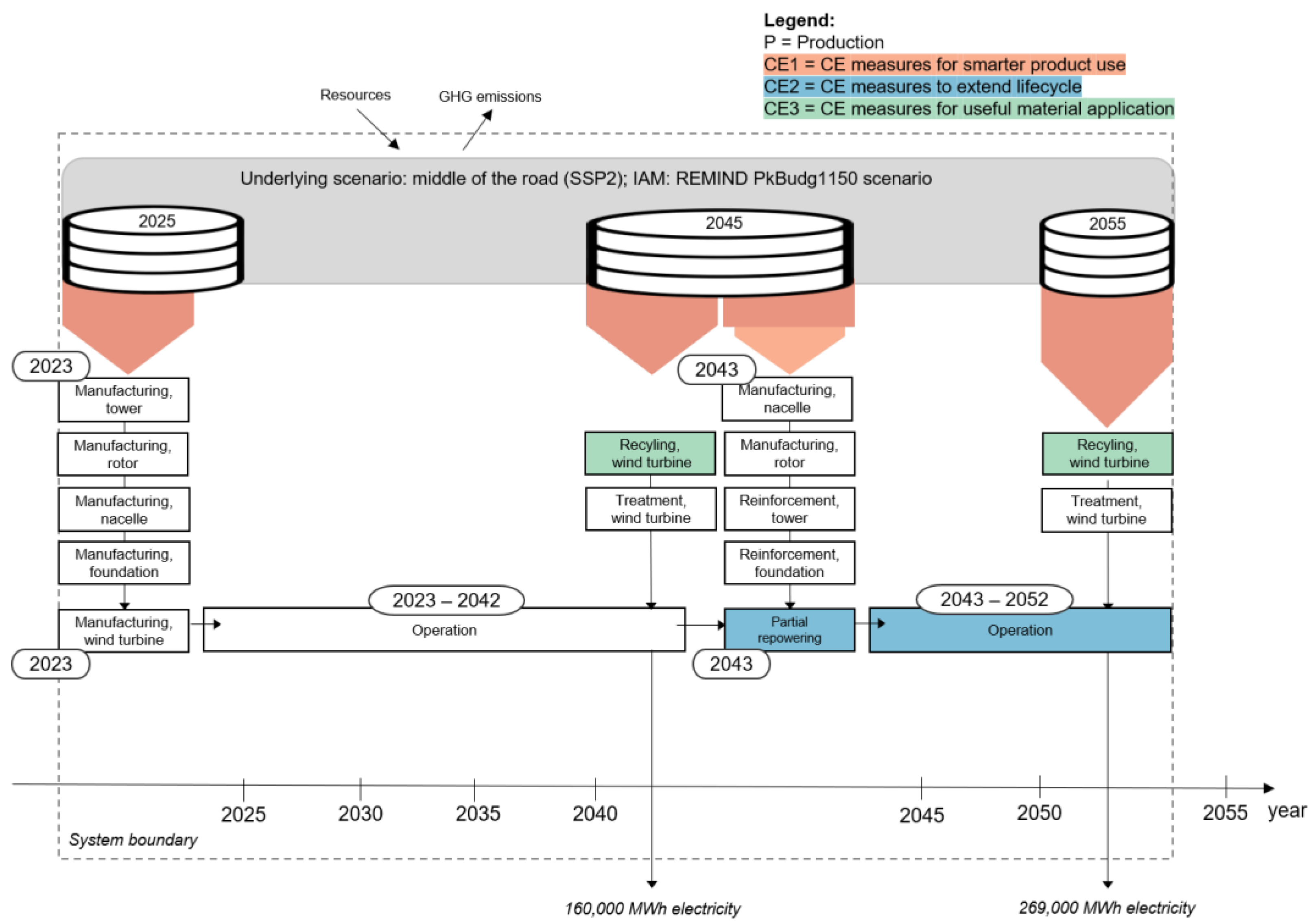
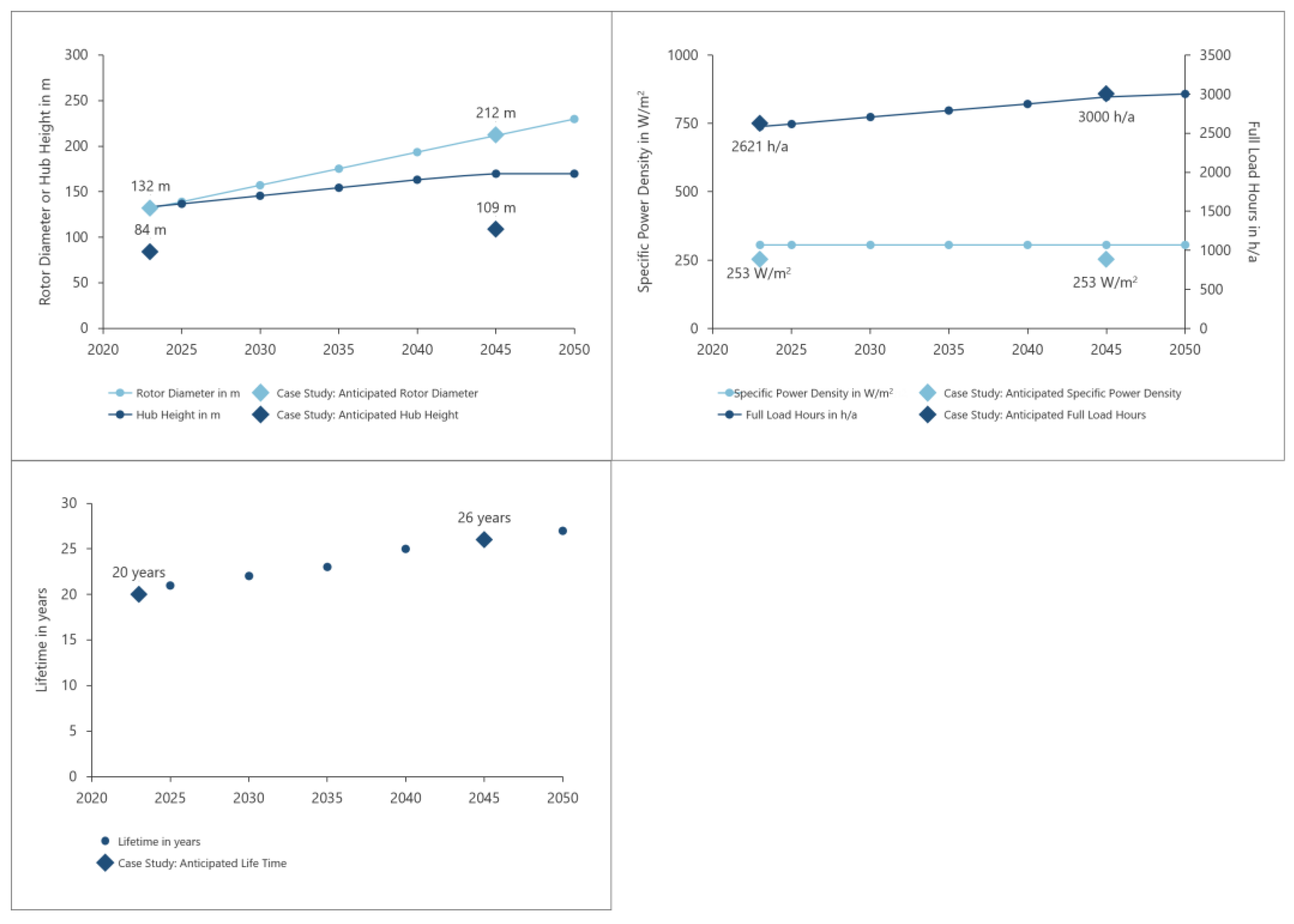
2.3. Goal of the Case Study

Finally, we applied this method to a case study. First, we assessed the life cycle impacts on the GWP of a partial repowering measure for a 3.3 Megawatt [MW] double-fed induction generator (GB-DFIG) onshore wind turbine. Considering that available land is a constraint to wind park operators who aim to maximize the amount of electricity generated from the available land, this measure was compared against the full repowering of the wind turbine. This case includes all three CE strategies: CE1 because technical optimizations leading to higher material efficiency are considered; CE2 because the repowering strategies represent lifetime-extending CE strategies of wind turbines; and CE3 because material recycling of the outdated components from the repowering is also included. Beyond that, the manufacturing and repowering of wind turbines represent a case with very long time spans and thus requires a dLCA approach to account for the product system’s evolution over time. Further, for the future, technological as well as market changes in the foreground and background are expected and should be considered. Hence, an integration of pLCA elements into a dLCA approach is needed.

3. Results

In this section, we present the results of the assessment of the partial repowering of the wind turbine and compare it to that with full repowering. We applied the method described in Section 2.2, which integrates elements from dLCA and pLCA. This case study is structured as follows: the goal and scope definitions are given in Section 3.1, the inventory analysis is detailed in Section 3.2, and the interpretation of the results is described in Section 3.3.

3.1. Goal and Scope

This case study aimed to answer the questions of whether and how much the implementation of partial repowering for a 3.3 MW GB-DFIG onshore wind turbine leads to a decrease in GWP. Further, it aimed to compare this effect with that of a full repowering of the wind turbine. The purpose of an onshore wind turbine is energy generation. Therefore, the generation of 1 kWh of electricity during the time from 2023 to 2052 was chosen as the functional unit and was not complemented by additional functions in the future. That means the benefits of the product system extended over the entire period and were considered cumulatively, calculated as a time-based average.

The life-cycle GHG emissions were taken into account, including the manufacturing of the wind turbine, as well as the recycling, replacement, and reinforcement of the components. Repair and maintenance activities were not included. The temporal scope of this work aligned with the functional unit and covered a period of 30 years from 2023 to 2052. The impact assessment focused on the impact category of climate change. The IPCC 2021 no LT GWP100 method (no LT = no long-term emissions) [56] was selected to assess the impact on climate change for this study, which does not consider dynamization. The projected number of wind turbines reflects the wind power capacity expansion plans of the German government to achieve its electricity decarbonization goals [57]. This is why the future electricity mix used in this study was based on results of the solidEU scenario [58]. The solidEU scenario represents a pathway where the greenhouse gas emissions (across all sectors) of European countries are reduced by 95% in 2050 compared to 1990. These developments for the energy system assume compliance with the Paris agreement objective, yet rely on an extrapolation from historical trends concerning human and economic development. Consequently, the solidEU scenario used in this study aligns with the SSP2 scenario, often postulated as “middle of the road” scenario. This underlying scenario served as a basis for the projections in the foreground and background system.

The impact of two commonly implemented strategies, partial repowering and full repowering, was examined. The scope of the partial repowering is illustrated in the system boundary diagram in Figure 2. In each case, the first wind turbine is built in 2023, has a lifetime of 20 years and will reach its end of life in 2042. In the case of partial repowering, the lifetime-limiting nacelle and rotor components are replaced by the newest technology. This upgrade requires reinforcing both the tower and the foundation. Due to the upgrade, the wind turbine becomes larger and is therefore able to generate a higher amount of electricity. This measure extends the operating lifetime by 10 years until 2052. When full repowering is applied, the wind turbine is completely decommissioned at the end of its lifetime and replaced by a wind turbine with the newest technology. Considering future developments, the newly built wind turbine has a lifetime of 26 years and will extend the operating lifetime until 2069. Considering the temporal system boundary (2023–2052), only the first 10 years of the newly built wind turbine are covered. The remaining 16 years of the wind turbine’s second operating lifetime are not part of the temporal system boundary. The two strategies analyzed in this case study are already being used by well-established wind turbine manufacturers [59]. Further, GB-DFIG wind turbines are holding an average market share of 29% of the onshore wind turbines in Europe in 2023 [2] and will still be part on the market at least until 2048. Besides the extension of the lifetime of the major components of the wind turbine for partial repowering, the recycling of the components is considered for both product systems and measures for smarter product use are implemented, since the material efficiency per electricity generated increased. The projected technological improvements are expected to be economically viable and widely used in the year 2043. The product system was set up for the German production; thus, the geographical system boundary remains constant within the system boundary. Since the considered emissions are restricted to the temporal scope of the study (30 years until 2052), only the share of the temporal system boundary was taken into account, even if data are collected with respect to the entire operating lifetime of a wind turbine. This is especially important for full repowering: the newly built wind turbine will extend the operating lifetime for 26 years, of which, only 10 years fall within the temporal system boundary of 30 years. Hence, all the emissions from the construction of the plant in 2042 and at the end of life in 2069 were accounted for but weighted by the share of the kWh of electricity generated during the time included in the system boundary relative to the total kWh of electricity generated during the temporal system boundary of 30 years.

3.2. Life Cycle Inventory

3.2.1. Foreground System

The inputs and outputs of each process in the foreground system were based on Schreiber et al. [60]. The onshore wind turbine analyzed in this case study was built in 2023 and has a rotor diameter of 132 m and a hub height (height of rotor above the ground) of 84 m. With a nominal power of 3.3 MW, the examined wind turbine will generate around 160 GWh electricity over its 20-year lifetime. The amount of electricity generated per year [MWh/a] is directly linked to the size of the rotor blades and was calculated by multiplying the rated power [MW] by the number of full load hours [h] [61]. The rated power [MW] can be derived from multiplying the area covered by the wind turbine [m²] by the specific nominal power density of the wind turbine [W/m²]. The area covered can be obtained from multiplying π by the square of the radius [m]. From this information, the LCI for the time between 2023 and 2043 was determined. Recycling was assumed for the steel, aluminum, and copper and was modeled based on the data from Schreiber et al. [60] and applying the cut-off approach. End-of-life recycling rates of 90% for steel, 92% for aluminum, and 95% for copper (except for cables) were used. Schreiber et al. [60] assumed high recycling rates, reasoning that wind turbines can be easily demolished and their materials are largely homogeneous. Blade recycling was modeled with data from Chiesura et al. [62], with 90% going to landfills and 10% being incinerated.

For the LCI of the investigated cases, future developments need to be taken into account, which were integrated in the LCA by adapting the foreground processes that represent the current technological and market status. Onshore wind turbines are expected to become larger, more efficient, and more durable. Hence, these foreground adaptions include changes in the material flows and the generated electricity over the lifetime due to the expected technology developments and the adaption of the electricity mix. In addition to implementing a future electricity mix, the case study included projected changes from several future technological trends, including changes in the rotor diameter, hub height, specific power density, number of full load hours, and lifetime. Both the LCI for 2023 and its future trends were validated by an expert of a wind turbine manufacturing company. This validation included an adjustment of the processes and quantities. In addition, the material flows that were grouped into nacelle and rotor in Schreiber et al. [60] were separated into nacelle and rotor. For confidentiality reasons, the validated LCI is not published in this paper. Figure 3 shows the assumed technological trends regarding onshore wind turbines. It is important to note that these developments are not certain developments but assumptions given the underlying scenario. By 2050, the size of the rotor blades is expected to increase to up to 230 m and the hub height to up to 170 m [61]. For the hub height, the predictions for the future have already assumed a higher hub starting point compared to the hub height of the wind turbine published in Schreiber et al. [60]. Hence, we considered the same level of relative development but starting and arriving at lower hub height numbers (see diagram on the left in Figure 3). Beyond that, it is assumed that by 2050, the number of full load hours will increase up to 3000 h/a and the specific power density will increase up to 304.75 W/m² [61]. It can also be predicted that the lifetime will increase from 20 years in 2023 to 29 years in 2050 [17]. Following these technological trends, the prospective assumptions were that a wind turbine built in 2043 (at the same location and under the same conditions) will have a rotor diameter of 212 m, a hub height of 108 m, and a lifetime of 26 years, and will generate 857 GWh of electricity over its lifetime. Based on the scaling formula from Caduff et al. [63], conclusions can be drawn from the size of the wind turbine for the corresponding mass change. Further, the electricity used for manufacturing the nacelle and rotor changes over time. A more detailed explanation of the implementation of the electricity mix based on the solidEU scenario can be found in Kilb and Haas [64].

3.2.2. Background System

The ecoinvent database 3.9.1 was chosen to represent the background of the product system. In order to take future developments into account, a prospective adaptation of the background database with the tool premise [40] was conducted, as described in Section 2.2. As there are various IAMs and a number of different scenarios, both the IAM and the IAM scenario selected for the background adaption were chosen based on the underlying scenario in this case study. Since our choice of the underlying scenario was mostly concerned with aligning similar target temperatures for global warming and the German electricity mix projections of a successful electricity transformation, we analyzed the IAM scenarios for the best fit with the solidEU projections [58]. This analysis resulted in the selection of the IAM REMIND and its scenario PkBudg1150 that aligns with projections for a global mean surface temperature increase of 1.6–1.8 °C by the year 2100 compared to pre-industrial levels [65] to best represent the development projected by the solidEU scenario. Since many future projections are available on a five-year basis, we followed the recommendations from Section 2.2 and transformed the ecoinvent database to represent five-year steps. Therefore, the database of the year 2035 describes the future projections for the period between 2031 and 2035.

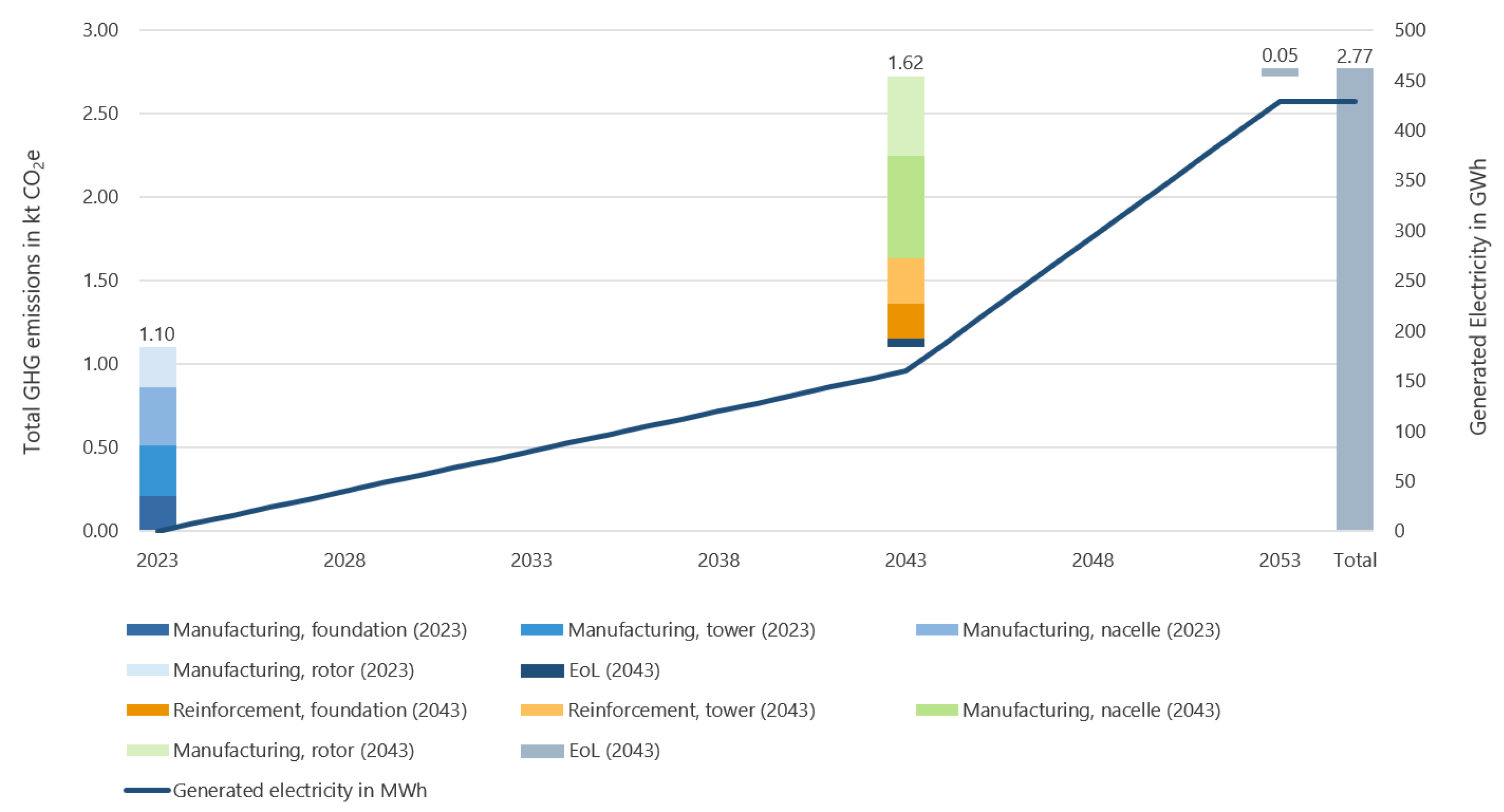
3.3. Life Cycle Impact Assessment and Interpretation

In the first step, the total GHG emissions and electricity generation were depicted over time for both cases. This approach allows for the illustration of the extent to which the cases diverge in terms of their total GHG emissions and total kWh of electricity generated. Secondly, in order to assess the actual environmental impact of the scenarios, it is essential to determine the GHG emissions produced in the generation of the functional unit, namely one kWh of electricity generated over the period from 2023 to 2053. This allows for a comparison of the GWP of the two cases, with the aim of determining which case results in the lowest specific emissions over the upcoming thirty years. The results hold true under consideration of the projected developments of the SSP2 scenario, meaning a “middle of the road” path that aligns with the Paris Agreement.

3.3.1. Total GHG Emissions and Total Electricity Produced

The results for the total GHG emissions and the time at which they occur are illustrated in Figure 4 for partial repowering and in Figure 5 for full repowering. For the case of partial repowering, the total GHG emissions over the entire operating lifetime were comparatively lower (2.8 kt CO₂e) than in the case full repowering (3.2 kt CO₂e). Based on these results, it can initially be concluded that partial repowering is the preferred measure from the perspective of total emissions. This partial repowering only completely replaced the nacelle and rotor in 2043 and extended the life of the other components through reinforcing them. Due to reinforcing the discarded wind turbine (partial repowering) or replacing the entire wind turbine (full repowering) with the newest technology, both product systems produced the same amount of electricity within the temporal system boundary of 30 years (429 GWh). It was further found (see Figure 5, dotted line) that the full repowering case could produce an additional 431 GWh of electricity in its operating lifetime of sixteen years beyond the temporal system boundary.

3.3.2. Global Warming Potential

The GWP of producing the functional unit, namely one kWh of electricity, is shown in Figure 6. Furthermore, the contribution of the individual components that were added to the product system over the course of time are displayed. It is shown that the case of partial repowering was associated with a higher specific emissions of 6.4 g CO₂e/kWh of produced electricity compared to the full repowering’s emissions of 4.5 g CO₂e/kWh. The GWP of the partial repowering contained contributions from the processes related to the manufacturing of the wind turbine built in 2023, including the manufacturing of the nacelle, rotor, foundation, and tower, and the processes related to the partial repowering, including the manufacturing of the new nacelle and rotor in 2043, the end of life of the discarded nacelle and rotor in 2043, the end of life of the remaining wind turbine components in 2053, as well as the reinforcement of the foundation and the tower. This reinforcement is necessary to ensure that the nacelle and rotor can be manufactured in accordance to the newest technology. The contributions of the nacelle (22%) and rotor (17%) manufactured in 2043 represent the highest contributions to the GWP.

In the case of full repowering, the contributions to the GWP corresponding to the manufacturing of the components of the wind turbine in 2023 are the same as those in the case of partial manufacturing. In contrast, the contributions to the GWP corresponding to the manufacturing of the components in 2043 were lower than those in the case partial repowering. Although the wind turbine built in 2043 generated the same amount of kWh electricity, the contribution to the GWP was lower. This effect can be attributed to the fact that the wind turbine in the case of full repowering has an operational lifetime of 26 years (instead of 10 years as in the case of partial repowering) and therefore, results in lower relative emissions since the overall emissions are partially allocated to the time after 2053. The results were obtained under the assumption of a “middle of the road” scenario, which is reflected in the performance and lifetime increases of the wind turbines after the repowering, as well as the decarbonized background during the repowering process, aligning with the Paris Agreement.

Considering these effects of the underlying assumptions, it can be concluded from comparing the GWP of the case of partial repowering and the case of full repowering that the full repowering achieved a better result of an approximately 30% lower GWP compared to the partial repowering. This outcome is mainly caused by the lifetime-extending effect of the full repowering scenario, which resulted in 26 years of additional operation of the wind turbine. It can theoretically produce electricity for an additional 16 years beyond the temporal system boundary, and thus generate an additional 431 GWh of electricity, 100% more electricity than the wind turbine in the partial repowering scenario. This compensates for the higher impacts due to the repowering process.

To summarize, although full repowering showed higher total GHG emissions, it still had the highest potential for reducing GHG emissions per kWh of generated electricity given the underlying assumptions due to its comparatively high electricity generation within the temporal system boundary as well as its electricity generation potential beyond the temporal system boundary.

4. Discussion

Given the scarcity of land designated to wind turbines, the objective is to achieve the greatest possible energy output per unit of available land, while minimizing the environmental impact. The method proposed in this study provides a useful basis for an assessment of CE strategies applied to a wind turbine, which explicitly differentiates time and takes into account future technological and market developments. The applied differentiation of time in the LCA and the inclusion of future developments via the use of pLCA is also useful for addressing the question of the most suitable timing for implementing a CE measure from the perspective of minimizing the GWP. This aspect is of great relevance to current wind turbine operators. As long as the expansion of wind turbines in Germany remains a political goal [57,66], our analysis indicates that full repowering should be prioritized, both from the perspective of contributing to the electricity transition and reducing the GWP per kWh generated. Furthermore, dLCA can help to calculate the break-even points for the GWP and include it into decision-making. In the future, as the transition to a decarbonized electricity mix progresses and additional wind capacity no longer directly avoids GWP-intensive electricity production elsewhere, implementing CE measures to extend the operational lifespan of existing infrastructure may still be justifiable. Such measures could lead to an overall reduction in GWP.

Developing a pLCA can be highly resource-intensive, and creating assessments for multiple time points, despite the proposed simplification to five-year intervals, significantly increases the effort required. Linear interpolations, as applied in our case study, offer a substantially simplified approach to projecting developments. However, constraints on technology deployment and market introduction, such as the earliest possible upscaling dates, must be considered and must remain consistent with the underlying scenario. In this study, for instance, the development of the wind turbine’s hub height is expected to reach a plateau due to operational feasibility, regulatory constraints, and decreasing effectiveness of height increases. The electricity mix was modeled based on cost-optimized expansion targets of energy technologies to achieve the German decarbonization goals for the electricity sector [57]. Alternatively, the forecasted development could rely on projections from German steel producers regarding the market implementation of direct reduction technologies, coupled with coal phase-out scenarios (as applied by Harpprecht et al. [52]). A systematic proposal for aligning the dynamics between the foreground and background systems would be helpful in this context.

At the same time, these considerations underscore the significant influence of the underlying scenario selection on LCI development. In the examined cases, the context of a successful energy transition in Germany aligned with the Paris Agreement goals was assumed. Thus, selecting the SSP2 and PkBudg1150 scenario appears justified, with both ecoinvent modifications using premise and foreground changes that align with these scenarios. However, achieving these goals cannot be taken for granted, especially in a global context or in highly emitting sectors such as housing and mobility within Germany. This uncertainty is illustrated by events such as the United States’ lack of reliability in committing to the Paris Agreement [67], the insufficient actions outlined in the existing Nationally Determined Contributions of its signatories [68], or the German cancellation of sector-specific monitoring as an indicator for determining sector-specific emergency measures [69]. This is why it is important to highlight under which assumptions of future developments the results have been obtained.

Beyond these uncertainties across various PESTEL categories, coupling with IAMs and the use of premise comes with inherent limitations. Most notably, the authors of premise [40] point out potential discrepancies between IAM regions and LCIs regarding the technologies and geographical boundaries considered. The granularity of the data varies, and assigning IAM data to ecoinvent cannot entirely resolve these differences. Additionally, LCIs can account for efficiency improvements and new processes, but disruptive future changes are challenging to capture. Consequently, the tool is recommended primarily for analyses extending to 2050–2060, even though IAMs might cover longer periods. Furthermore, de Bortoli [70] noted that despite the widespread use of IAMs in pLCA, the LCA community does not yet fully understand IAMs and their underlying logic. For instance, she elaborated that most IAMs are grounded in neoclassical economic theories, emphasizing the supply side. This highlights the importance of thoroughly interpreting results while focusing on the origin of relative differences. Moreover, testing the robustness of results using different IAMs and an alternative underlying scenario is strongly recommended.

One important drawback of the simplicity of the presented methodological approach is its partial dynamization. The elementary flows are not temporally differentiated, which precludes the possibility of conducting a dynamic LCIA with time-specific characterization factors. Therefore, the impact assessment is consistent with the static LCA approach, wherein all emissions for a given pollutant are aggregated into a single value in the LCI, irrespective of the time of occurrence [71]. In the present case of the repowering scenarios, the main contributing elementary flow was CO₂. The significance of other greenhouse gases in the assessment of the GWP was negligible, and each kilogram of CO₂ was calculated with a factor of exactly 1 kg CO₂e, irrespective of whether a finite time horizon was considered (e.g., only the climate impact up to 2070 is to be taken into account) or not. However, adopting the position that 100 years of climate impact should always be considered could allow for the discounting of future emissions (as applied by Zhang [72]). This approach, influenced by the principles of financial accounting, may be driven by higher uncertainties surrounding future developments or a greater emphasis on the needs of current generations. In this case, study, full repowering would prove to be even more advantageous than partial repowering, as the higher absolute emissions due to new construction instead of reinforcement that occurs at a later stage (2042) is weighted lower by discounting. Consequently, the efficiency of the GWP per unit of electricity produced would decrease more proportionately than in the partial repowering scenario.

Although this type of limitation due to partial dynamization has been accepted by numerous case studies [20], there are now more possibilities as more sophisticated tools to dynamize the LCI and compute a dynamic LCIA, including applying dynamic characterization factors, have been developed. For instance, the approach by Tiruta-Barna et al. [32] uses a process flow network structure and graph search algorithms to build temporal models, creating a basis for further software development [32,73]. The software Temporalis [33] facilitates temporally differentiated LCIs through graph traversal and convolution, enabling dynamic LCIA. The recently introduced Python-based tool bw_timex [74] integrates these advancements and links future LCIs with databases modified by premise in the background. This allows for the modeling, computation, and analysis of far more complex case studies than those presented here, which address the beforementioned shortcomings. In contrast, the method presented here presents a simplified solution that could also be deployed outside the bw2 ecosystem, contingent on the availability of temporal emission factors from premise. Nevertheless, this would entail a considerable loss of information with regard to the supply chains. In conclusion, the presented method represents a practical and straightforward solution, while bw_timex offers a fully dynamic LCA approach and has substantial potential for future application.

Ultimately, the accessibility of data for future technological and market developments remains a key challenge. This is especially the case with impact categories beyond climate change, which are also important when comprehensively assessing energy infrastructure, such as land use or water scarcity to name a few. An intriguing approach could be coupling with material flow models (e.g., [5]) in order to better represent substitution factors and future recycling rates when assessing CE measures.

5. Conclusions

To date, in the context of CE measure evaluation, LCA studies have either not incorporated time differentiation or have inadequately addressed the future developments that influence CE measures. The present paper proposes an extended LCA method to integrate advancements made for future-oriented LCA into each step of the dLCA framework. The methodology provides recommendations for all major steps of an LCA, thus enabling consideration of technological, market, and supply chain developments in the LCI of a study. This approach enables the consideration of substantial modifications and prevents erroneous conclusions regarding the (dis)advantages of product features of long-lived products. Consequently, this approach provides a foundation for evaluating CE strategies as it enables the temporal differentiation between the initial production phase and the timing of CE measures, along with their potentially altered LCIs. This extended LCA approach is a prerequisite for various types of CE strategies. Strategies that are designed to extend the lifespan of a product and its components (referred to as CE2 strategies) typically center around two key points in the product’s life cycle: the time of production and the time of the implementation of the CE measure. It is very likely that a technological and market development will occur in the interim in the foreground and background, and these should be adequately addressed. In the context of CE3 strategies, the timing of the application of the material is relevant too. Conversely, strategies that aim for smarter product use and manufacturing (herein called CE1 strategies) require a continuous representation of the temporal dynamics. This poses a distinctive challenge as prospective developments at both the technological and market levels must be forecast not only for a single future point but for multiple ones. This applies, for instance, to inputs during the long use phase of machinery [75], wherein life cycle impacts may dynamically evolve and consequently require incorporation into the assessment.

The method was employed to analyze the GWP of two distinct CE measures on wind turbines, applying the procedure for the goal and scope and LCI, as well as the interpretation of the results. Given the longevity of wind turbines, life-extending measures such as partial repowering and the recycling of dismantled materials are implemented only in the distant future, typically a minimum of twenty years after the initial installation. A comparison of full repowering with partial repowering was conducted, revealing that full repowering is the preferred option from a GWP perspective, due to the larger amounts of electricity produced after the introduction of the measure in 2042. Compared to the partial repowering case, the higher absolute emissions resulting from the demolition, recycling, and new construction of the new plant resulted in a higher benefit according to the findings of this study. The technological progress and the decarbonization assumed in the underlying scenario in accordance with the Paris climate targets contributed to these results. Even when weighting methods such as discounting emissions in the more distant future were applied, these results remained robust or were even reinforced. While the study acknowledges limitations in fully dynamic impact assessments, it highlights the potential of emerging tools such as bw_timex to address these challenges. The proposed method is straightforward to apply and can be adapted for LCAs of long-lasting products, including planned CE measures, as demonstrated by Kilb and Haas [64]. It would be useful to have further LCA studies that more broadly investigate the use of this integrated approach versus the state of the art to demonstrate the quantitative effects and associated changes for the derived conclusions.

References

1. Cozzi, L.; Gül, T.; Fernández, A.; Spencer, T.; Bouckaert, S.; McGlade, C.; Remme, U.; Wanner, B.; D’Ambrosio, D.e.a. Net Zero Roadmap: A Global Pathway to Keep the 1.5 °C Goal in Reach: 2023 Update. 2023. Available online: https://iea.blob.core.windows.net/assets/9a698da4-4002-4e53-8ef3-631d8971bf84/NetZeroRoadmap_AGlobalPathwaytoKeepthe1.5CGoalinReach-2023Update.pdf (accessed on 27 September 2024).
2. Carrara, S.; Alves Dias, P.; Pazzotta, B.; Pavel, C. Raw Materials Demand for Wind and Solar PV Technologies in the Transition To-wards a Decarbonised Energy System, EUR 30095 EN; European Union: Luxembourg, 2020. [Google Scholar]
3. European Union. Study on the Critical Raw Materials for the EU 2023: Final Report; European Union: Luxembourg, 2023. [Google Scholar]
4. Charpentier Poncelet, A.; Helbig, C.; Loubet, P.; Beylot, A.; Muller, S.; Villeneuve, J.; Laratte, B.; Thorenz, A.; Tuma, A.; Sonnemann, G. Losses and lifetimes of metals in the economy. Nat. Sustain. 2022, 5, 717–726. [Google Scholar] [CrossRef]
5. Buchert, M.; Bleher, D.; Bulach, W.; Knappe, F.; Muchow, N.; Reinhardt, J.; Meinshausen, I. Kartierung des Anthropogenen Lagers III (KartAL III); Abschlussbericht; UBA-Texte 47/2022; Umweltbundesamt: Dessau-Roßlau, Germany, 2022. [Google Scholar]
6. Kirchherr, J.; Reike, D.; Hekkert, M. Conceptualizing the circular economy: An analysis of 114 definitions. Resour. Conserv. Recycl. 2017, 127, 221–232. [Google Scholar] [CrossRef]
7. Potting, J.; Hekkert, M.; Worrell, E.; Hanemaaijer, A. Circular Economy: Measuring Innovation in the Product Chain: Policy Report; PBL Netherlands Environmental Assessment Agency: The Hague, The Netherlands, 2017. [Google Scholar]
8. Gebhardt, M.; Spieske, A.; Birkel, H. The future of the circular economy and its effect on supply chain dependencies: Empirical evidence from a Delphi study. Transp. Res. Part E Logist. Transp. Rev. 2022, 157, 102570. [Google Scholar] [CrossRef]
9. Hagelücken, C.; Schmidt, M.; Schebek, L.; Liedtke, C.; Bongardt, B.; Dosch, K.; Faulstich, M.; Flamme, S.; Gast, M.; Hermann, S.; et al. Chancen und Grenzen des Recyclings im Kontext der Circular Economy: Rahmenbedingungen, Anforderungen und Handlungsempfehlungen. 2023. Available online: https://www.umweltbundesamt.de/sites/default/files/medien/1410/publikationen/2023_uba_kom_ressourcen_bf.pdf (accessed on 3 February 2025).
10. Schäfer, P. Recycling—Ein Mittel zu Welchem Zweck? Springer Fachmedien Wiesbaden: Wiesbaden, Germany, 2021; ISBN 978-3-658-32923-5. [Google Scholar]
11. Reuter, M.A.; van Schaik, A.; Gutzmer, J.; Bartie, N.; Abadías-Llamas, A. Challenges of the Circular Economy: A Material, Metallurgical, and Product Design Perspective. Annu. Rev. Mater. Res. 2019, 49, 253–274. [Google Scholar] [CrossRef]
12. Law for the Expansion of Renewable Energies: EEG. 2023. Available online: https://climate-laws.org/document/renewable-energy-sources-act-eeg-latest-version-eeg-2022_1b40 (accessed on 9 December 2024).
13. Doukas, H.; Arsenopoulos, A.; Lazoglou, M.; Nikas, A.; Flamos, A. Wind repowering: Unveiling a hidden asset. Renew. Sustain. Energy Rev. 2022, 162, 112457. [Google Scholar] [CrossRef]
14. Fuchs, C.; Kasten, J.; Vent, M. Current State and Future Prospective of Repowering Wind Turbines: An Economic Analysis. Energies 2020, 13, 3048. [Google Scholar] [CrossRef]
15. ISO 14044:2006; Environmental Management—Life Cycle Assessment—Requirements and Guidelines. International Organization for Standardization: Geneva, Swtizerland, 2006.
16. ISO 14040:2006; Environmental Management—Life Cycle Assessment—Principles and Framework. International Organization for Standardization: Geneva, Swtizerland, 2006.
17. Li, H.; Jiang, H.-D.; Dong, K.-Y.; Wei, Y.-M.; Liao, H. A comparative analysis of the life cycle environmental emissions from wind and coal power: Evidence from China. J. Clean. Prod. 2020, 248, 119192. [Google Scholar] [CrossRef]
18. Danish Energy Agency. Technology Data for Transport of Energy: Data Sheets for Transport of Energy. Excel File. Available online: https://ens.dk/en/analyses-and-statistics/technology-data-transport-energy (accessed on 5 June 2024).
19. Ajeeb, W.; Costa Neto, R.; Baptista, P. Life cycle assessment of green hydrogen production through electrolysis: A literature review. Sustain. Energy Technol. Assess. 2024, 69, 103923. [Google Scholar] [CrossRef]
20. Sohn, J.; Kalbar, P.; Goldstein, B.; Birkved, M. Defining Temporally Dynamic Life Cycle Assessment: A Review. Integr. Environ. Assess. Manag. 2020, 16, 314–323. [Google Scholar] [CrossRef]
21. Pehnt, M. Dynamic life cycle assessment (LCA) of renewable energy technologies. Renew. Energy 2006, 31, 55–71. [Google Scholar] [CrossRef]
22. Collinge, W.O.; Landis, A.E.; Jones, A.K.; Schaefer, L.A.; Bilec, M.M. Dynamic life cycle assessment: Framework and application to an institutional building. Int. J. Life Cycle Assess. 2013, 18, 538–552. [Google Scholar] [CrossRef]
23. Arvidsson, R.; Svanström, M.; Sandén, B.A.; Thonemann, N.; Steubing, B.; Cucurachi, S. Terminology for future-oriented life cycle assessment: Review and recommendations. Int. J. Life Cycle Assess. 2024, 29, 607–613. [Google Scholar] [CrossRef]
24. Cucurachi, S.; van der Giesen, C.; Guinée, J. Ex-ante LCA of Emerging Technologies. Procedia CIRP 2018, 69, 463–468. [Google Scholar] [CrossRef]
25. Arvidsson, R.; Tillman, A.-M.; Sandén, B.A.; Janssen, M.; Nordelöf, A.; Kushnir, D.; Molander, S. Environmental Assessment of Emerging Technologies: Recommendations for Prospective LCA. J. Ind. Ecol. 2018, 22, 1286–1294. [Google Scholar] [CrossRef]
26. Bergerson, J.A.; Brandt, A.; Cresko, J.; Carbajales-Dale, M.; MacLean, H.L.; Matthews, H.; McCoy, S.; McManus, M.; Miller, S.A.; Morrow, W.R.I.; et al. Life cycle assessment of emerging technologies: Evaluation techniques at different stages of market and technical maturity. J. Ind. Ecol. 2020, 24, 11–25. [Google Scholar] [CrossRef]
27. Guinée, J.B.; Cucurachi, S.; Henriksson, P.J.; Heijungs, R. Digesting the alphabet soup of LCA. Int. J. Life Cycle Assess. 2018, 23, 1507–1511. [Google Scholar] [CrossRef]
28. Weyand, S.; Kawajiri, K.; Mortan, C.; Schebek, L. Scheme for generating upscaling scenarios of emerging functional materials based energy technologies in prospective LCA (UpFunMatLCA). J. Ind. Ecol. 2023, 27, 676–692. [Google Scholar] [CrossRef]
29. Tsoy, N.; Steubing, B.; van der Giesen, C.; Guinée, J. Upscaling methods used in ex ante life cycle assessment of emerging technologies: A review. Int. J. Life Cycle Assess. 2020, 25, 1680–1692. [Google Scholar] [CrossRef]
30. Piccinno, F.; Hischier, R.; Seeger, S.; Som, C. From laboratory to industrial scale: A scale-up framework for chemical processes in life cycle assessment studies. J. Clean. Prod. 2016, 135, 1085–1097. [Google Scholar] [CrossRef]
31. Su, S.; Ju, J.; Ding, Y.; Yuan, J.; Cui, P. A Comprehensive Dynamic Life Cycle Assessment Model: Considering Temporally and Spatially Dependent Variations. Int. J. Environ. Res. Public Health 2022, 19, 14000. [Google Scholar] [CrossRef]
32. Tiruta-Barna, L.; Pigné, Y.; Navarrete Gutiérrez, T.; Benetto, E. Framework and computational tool for the consideration of time dependency in Life Cycle Inventory: Proof of concept. J. Clean. Prod. 2016, 116, 198–206. [Google Scholar] [CrossRef]
33. Cardellini, G.; Mutel, C.L.; Vial, E.; Muys, B. Temporalis, a generic method and tool for dynamic Life Cycle Assessment. Sci. Total Environ. 2018, 645, 585–595. [Google Scholar] [CrossRef]
34. Levasseur, A.; Lesage, P.; Margni, M.; Deschênes, L.; Samson, R. Considering time in LCA: Dynamic LCA and its application to global warming impact assessments. Environ. Sci. Technol. 2010, 44, 3169–3174. [Google Scholar] [CrossRef]
35. Østergaard, N.; Thorsted, L.; Miraglia, S.; Birkved, M.; Rasmussen, F.N.; Birgisdóttir, H.; Kalbar, P.; Georgiadis, S. Data Driven Quantification of the Temporal Scope of Building LCAs. Procedia CIRP 2018, 69, 224–229. [Google Scholar] [CrossRef]
36. Mutel, C.L.; Hellweg, S. Regionalized life cycle assessment: Computational methodology and application to inventory databases. Environ. Sci. Technol. 2009, 43, 5797–5803. [Google Scholar] [CrossRef] [PubMed]
37. Thonemann, N.; Schulte, A.; Maga, D. How to Conduct Prospective Life Cycle Assessment for Emerging Technologies? A Systematic Review and Methodological Guidance. Sustainability 2020, 12, 1192. [Google Scholar] [CrossRef]
38. Langkau, S.; Steubing, B.; Mutel, C.; Ajie, M.P.; Erdmann, L.; Voglhuber-Slavinsky, A.; Janssen, M. A stepwise approach for Scenario-based Inventory Modelling for Prospective LCA (SIMPL). Int. J. Life Cycle Assess. 2023, 28, 1169–1193. [Google Scholar] [CrossRef]
39. Mendoza Beltran, A.; Cox, B.; Mutel, C.; Vuuren, D.P.; Font Vivanco, D.; Deetman, S.; Edelenbosch, O.Y.; Guinée, J.; Tukker, A. When the Background Matters: Using Scenarios from Integrated Assessment Models in Prospective Life Cycle Assessment. J. Ind. Ecol. 2020, 24, 64–79. [Google Scholar] [CrossRef]
40. Sacchi, R.; Terlouw, T.; Siala, K.; Dirnaichner, A.; Bauer, C.; Cox, B.; Mutel, C.; Daioglou, V.; Luderer, G. PRospective EnvironMental Impact asSEment (premise): A streamlined approach to producing databases for prospective life cycle assessment using integrated assessment models. Renew. Sustain. Energy Rev. 2022, 160, 112311. [Google Scholar] [CrossRef]
41. Riahi, K.; van Vuuren, D.P.; Kriegler, E.; Edmonds, J.; O’Neill, B.C.; Fujimori, S.; Bauer, N.; Calvin, K.; Dellink, R.; Fricko, O.; et al. The Shared Socioeconomic Pathways and their energy, land use, and greenhouse gas emissions implications: An overview. Glob. Environ. Chang. 2017, 42, 153–168. [Google Scholar] [CrossRef]
42. Schmidt, M.; Heidak, P. Intertemporal allocation of long-lasting recycling cascades. Energies 2025, Manuscript submitted for publication. [Google Scholar]
43. Issa, T.; Chang, V.; Issa, T. Sustainable business strategies and PESTEL framework. Int. J. Comput. 2010, 1, 73–80. [Google Scholar] [CrossRef]
44. Erakca, M.; Baumann, M.; Helbig, C.; Weil, M. Systematic review of scale-up methods for prospective life cycle assessment of emerging technologies. J. Clean. Prod. 2024, 451, 142161. [Google Scholar] [CrossRef]
45. Buyle, M.; Audenaert, A.; Billen, P.; Boonen, K.; van Passel, S. The Future of Ex-Ante LCA? Lessons Learned and Practical Recommendations. Sustainability 2019, 11, 5456. [Google Scholar] [CrossRef]
46. Ecoinvent. Ecoinvent Database. Available online: https://ecoinvent.org/database/ (accessed on 9 July 2024).
47. Mutel, C. Brightway: An open source framework for Life Cycle Assessment. JOSS 2017, 2, 236. [Google Scholar] [CrossRef]
48. Villares, M.; Işıldar, A.; van der Giesen, C.; Guinée, J. Does ex ante application enhance the usefulness of LCA? A case study on an emerging technology for metal recovery from e-waste. Int. J. Life Cycle Assess. 2017, 22, 1618–1633. [Google Scholar] [CrossRef]
49. Voglhuber-Slavinsky, A.; Zicari, A.; Smetana, S.; Moller, B.; Dönitz, E.; Vranken, L.; Zdravkovic, M.; Aganovic, K.; Bahrs, E. Setting life cycle assessment (LCA) in a future-oriented context: The combination of qualitative scenarios and LCA in the agri-food sector. Eur. J. Futures Res. 2022, 10, 15. [Google Scholar] [CrossRef]
50. Weidema, B.P.; Bauer, C.; Hischier, R.; Mutel, C.; Nemecek, T.; Reinhard, J.; Vadenbo, C.O.; Wernet, G. Overview and Methodology: Data Quality Guideline for the Ecoinvent Database Version 3. Ecoinvent Report No. 1(v3), St. Gallen. 2013. Available online: https://lca-net.com/publications/show/overview-methodology-data-quality-guideline-ecoinvent-database-version-3/ (accessed on 9 December 2024).
51. Virtuelles Institut Strom zu Gas und Wärme NRW. Abschlusszentrum Kompetenzzentrum Virtuelles Institut Strom zu Gas und Wärme: Band 2—Lebenszyklusorientierte Analysen und Kritikalitätsanalyse von Power-to-X-Optionen. 2022. Available online: https://strom-zu-gas-und-waerme.de/wp-content/uploads/2022/07/KoVI-SGW-Abschlussbericht-Band-II-M%C3%A4rz-2022-final.pdf (accessed on 7 October 2024).
52. Harpprecht, C.; Naegler, T.; Steubing, B.; Tukker, A.; Simon, S. Decarbonization scenarios for the iron and steel industry in context of a sectoral carbon budget: Germany as a case study. J. Clean. Prod. 2022, 380, 134846. [Google Scholar] [CrossRef]
53. Van der Meide, M.; Harpprecht, C.; Northey, S.; Yang, Y.; Steubing, B. Effects of the energy transition on environmental impacts of cobalt supply: A prospective life cycle assessment study on future supply of cobalt. J. Ind. Ecol. 2022, 26, 1631–1645. [Google Scholar] [CrossRef]
54. Scrucca, F.; Baldassarri, C.; Baldinelli, G.; Bonamente, E.; Rinaldi, S.; Rotili, A.; Barbanera, M. Uncertainty in LCA: An estimation of practitioner-related effects. J. Clean. Prod. 2020, 268, 122304. [Google Scholar] [CrossRef]
55. Heijungs, R.; Suh, S. The Computational Structure of LCA; Kluwer Academic Publishers: Dordrecht, The Netherlands, 2002. [Google Scholar]
56. Sonderegger, T.; Stoikou, N. Implementation of Life Cycle Impact Assessment Methods in the Ecoinvent Database v3.9; Ecoinvent: Zurich, Switzerland, 2022. [Google Scholar]
57. Federal Ministry for the Environment, Nature Conservation, Building and Nuclear Safety. Klimaschutzplan 2050: Klimaschutzpolitische Grundsätze und Ziele der Bundesregierung; Federal Ministry for the Environment, Nature Conservation, Building and Nuclear Safety: Berlin, Germany, 2016. [Google Scholar]
58. Kigle, S.; Ebner, M.; Guminski, A. Greenhouse Gas Abatement in EUROPE—A Scenario-Based, Bottom-Up Analysis Showing the Effect of Deep Emission Mitigation on the European Energy System. Energies 2022, 15, 1334. [Google Scholar] [CrossRef]
59. Siemens Gamesa. Spares and Repairs for Wind Turbines: Flexible Solutions to Support Performance and Reduce Downtime. Available online: https://www.siemensgamesa.com/global/en/home/products-and-services/service-wind/spares-and-repairs.html (accessed on 12 December 2024).
60. Schreiber, A.; Marx, J.; Zapp, P. Comparative life cycle assessment of electricity generation by different wind turbine types. J. Clean. Prod. 2019, 233, 561–572. [Google Scholar] [CrossRef]
61. Borrmann, R.; Rehfeldt, K.; Kruse, D. Volllaststunden von Windenergieanlagen an Land—Entwicklung, Einflüsse, Auswirkungen, Varel. 2020. Available online: https://www.windguard.de/veroeffentlichungen.html?file=files/cto_layout/img/unternehmen/veroeffentlichungen/2020/Volllaststunden%20von%20Windenergieanlagen%20an%20Land%202020.pdf (accessed on 7 October 2024).
62. Chiesura, G.; Stecher, H.; Pagh Jensen, J. Blade materials selection influence on sustainability: A case study through LCA. IOP Conf. Ser. Mater. Sci. Eng. 2020, 942, 12011. [Google Scholar] [CrossRef]
63. Caduff, M.; Huijbregts, M.A.J.; Althaus, H.-J.; Koehler, A.; Stefanie, H. Wind power electricity: The bigger the turbine, the greener the electricity? Environ. Sci. Technol. 2012, 46, 4725–4733. [Google Scholar] [CrossRef]
64. Kilb, J.; Haas, S. Analyzing the influence of implementing dynamic prospective research data in energy industry life cycle assessment based on a case study of a power transformer. Energies 2025, Manuscript submitted for publication. [Google Scholar]
65. Luderer, G.; Leimbach, M.; Bauer, N.; Kriegler, E.; Baumstark, L.; Bertram, C.; Giannousakis, A.; Hilaire, J.; Klein, D.; Levesque, A.; et al. Description of the REMIND Model (Version 1.6). SSRN J. 2015. [Google Scholar] [CrossRef]
66. German Federal Government. So Läuft der Ausbau der Erneuerbaren Energien in Deutschland. Available online: https://www.bundesregierung.de/breg-de/aktuelles/ausbau-erneuerbare-energien-2225808 (accessed on 20 February 2025).
67. Pompeo, M.R. On the U.S. Withdrawal from the Paris Agreement. 2019. Available online: https://2017-2021.state.gov/on-the-u-s-withdrawal-from-the-paris-agreement/ (accessed on 20 February 2025).
68. UNEP. Emissions Gap Report 2023: Broken Record—Temperatures Hit New Highs, Yet World Fails to Cut Emissions (Again), Nairobi. 2023. Available online: https://wedocs.unep.org/bitstream/handle/20.500.11822/43923/EGR2023_ESEN.pdf?sequence=10 (accessed on 9 December 2024).
69. Umweltbundesamt. Treibhausgasminderungsziele Deutschlands. Available online: https://www.umweltbundesamt.de/daten/klima/treibhausgasminderungsziele-deutschlands#internationale-vereinbarungen-weisen-den-weg (accessed on 20 February 2020).
70. De Bortoli, A. Strenghts, Limitations, and Perspectives of coupling IAMs and LCA to study feasible and desirable societal pathways. Seville, 7 May 2024.
71. Life-Cycle Impact Assessment: Striving Towards Best Practice; Haes, U., Helias, A., Eds.; SETAC Press: Pensacola, FL, USA, 2002; ISBN 9781880611548. [Google Scholar]
72. Zhang, Y. Taking the Time Characteristic into Account of Life Cycle Assessment: Method and Application for Buildings. Sustainability 2017, 9, 922. [Google Scholar] [CrossRef]
73. Pigné, Y.; Gutiérrez, T.N.; Gibon, T.; Schaubroeck, T.; Popovici, E.; Shimako, A.H.; Benetto, E.; Tiruta-Barna, L. A tool to operationalize dynamic LCA, including time differentiation on the complete background database. Int. J. Life Cycle Assess. 2020, 25, 267–279. [Google Scholar] [CrossRef]
74. Diepers, T.; Müller, A.; Jakobs, A. bw_timex: v0.3.1. Available online: https://docs.brightway.dev/projects/bw-timex/en/latest/ (accessed on 21 April 2025).
75. Kasah, T. LCA of a newsprint paper machine: A case study of capital equipment. Int. J. Life Cycle Assess. 2014, 19, 417–428. [Google Scholar] [CrossRef]
Figure 1. Example time-explicit system boundary diagram of an energy-generating plant.
Energies 18 02509 g001
Figure 2. Time-explicit system boundary diagram of electricity production from a wind turbine with partial repowering.
Energies 18 02509 g002
Figure 3. Assumed technology development for onshore wind turbine rotor diameter and hub height (first row, left), specific power density, full load hours (first row, right), and lifetime (second row, left) based on [61] and validated by an expert from a wind turbine manufacturing company.
Energies 18 02509 g003
Figure 4. Total GHG emissions in kt CO2e and total generated electricity in GWh for partial repowering.
Energies 18 02509 g004
Figure 5. Total GHG emissions in kt CO2e and total generated electricity in MWh for full repowering.
Energies 18 02509 g005
Figure 6. Environmental impact of partial repowering (left) and full repowering (right).
Energies 18 02509 g006
Disclaimer/Publisher’s Note: The statements, opinions and data contained in all publications are solely those of the individual author(s) and contributor(s) and not of MDPI and/or the editor(s). MDPI and/or the editor(s) disclaim responsibility for any injury to people or property resulting from any ideas, methods, instructions or products referred to in the content.