Research on High-Precision Calculation Method for Permanent Magnet Synchronous Motor Efficiency in Electric Vehicles Across Full Load-Speed Range

Abstract

In order to accurately calculate the efficiency of electric vehicle drive motors in the full speed range during the design phase, this paper proposes a comprehensive motor loss fast calculation method. Firstly, a high-fidelity joint simulation model of control and design was established to simulate the real excitation sources in actual operation. Secondly, detailed modeling was conducted for each loss. Regarding iron loss, this paper considers the effects of PWM harmonics, as well as cutting, welding, and other processes, on the loss based on finite element calculations. This paper proposes a semi-analytical AC copper loss calculation method, which superimposes the effective section and end winding separately. A fast improvement simulation method is proposed for the eddy current loss of permanent magnets, which equivalently combines 2D finite element and 3D finite element, while considering factors such as segmentation. Finally, a loss separation scheme was designed and experimentally verified for each loss and motor efficiency, proving that the efficiency calculation error of most operating points was less than 1.5%.

1. Introduction

Permanent magnet synchronous motors (PMSMs) have become the preferred solution for electric vehicle drive motors due to their advantages of high power density and high torque density [1]. With the pursuit of higher indicators, there is an increasing need for precise calculation of motor energy consumption to ensure safety and control boundaries. At the same time, rapid and accurate calculation of losses is of great significance for improving the overall energy efficiency of the vehicle, optimizing motor design, and extending the life of key components [2]. Therefore, there is an urgent need for a method that can accurately and relatively quickly calculate the energy consumption of electric vehicle drive motors under the entire operating condition during the motor design stage.

The losses of PMSMs are mainly divided into core losses, winding copper losses, permanent magnet eddy current losses, and mechanical losses. So far, a large number of researchers have conducted in-depth research on loss calculation and analysis. The iron core loss is mainly affected by time harmonics introduced by the PWM (pulse width modulation) inverter, as well as material characteristics and manufacturing process [3,4,5]. According to the mechanism of iron core loss, the mainstream calculation methods currently include classical analytical methods such as Steinmetz equation and Bertotti separation model [6,7], as well as the most commonly used FEM (finite element method), which has higher accuracy but longer time consumption [8]. If time harmonics need to be considered, the calculation time will be even longer. The calculation cases of iron core loss considering the process are even rarer, and further research is needed to improve accuracy.

Copper loss accounts for a large proportion of motor losses, especially under heavy load or low-speed conditions, and is basically the main source of motor losses. With the large-scale application of flat wires, the skin effect and proximity effect are becoming stronger, and the proportion of AC (alternating current) copper loss in the entire copper loss is increasing [9]. Therefore, in addition to calculating DC (direct current) copper loss, accurate calculation of AC copper loss is also needed. In addition, much of literatures focus on calculating the effective section and ignores the copper loss generated by the end winding [10,11]. At present, the main methods for calculating the losses of flat wire windings include FEM, analytical method, and semi analytical method. To achieve accurate loss calculation, the FEM must perform precise subdivision of the winding area. Although the calculation accuracy is high, the solution time is long, and it is difficult to meet the fast calculation requirements, such as multi-objective optimization [12]. The analytical model has been proposed to reduce the solving time. However, this type of method ignores the effects of iron core magnetic saturation and rotor magnetic field, resulting in significant calculation errors [13]. To compensate for the shortcomings of the above methods, the semi analytical method combining FEM with analytical expressions has become a research hotspot [14].

The permanent magnet eddy current loss is usually small, but it is often difficult to ignore in high-speed and heavy-duty conditions [15]. At the same time, accurate calculation of eddy current losses in permanent magnets lays the foundation for temperature monitoring and improves the reliability of the system. Due to its loss caused by harmonics, researchers typically focus on the effects of time and space harmonics on it [16,17]. In addition, due to the fact that automotive motors usually suppress torque ripple through segmented skewed poles, this has also become one of the factors affecting eddy current losses of permanent magnets [18,19]. At present, 2D FEM is difficult to accurately calculate the permanent magnet eddy current loss due to end effects, and 3D FEM is often the only way to accurately calculate the permanent magnet eddy current loss of interior PMSMs [20]. Some analytical formulas can accurately calculate the permanent magnet eddy current loss of surface-mounted PMSMs [21]. Moreover, the combination of FEM and analytical method is a development trend in order to balance calculation time and accuracy [22].

In conclusion, it is a huge challenge to calculate the full speed domain losses of the PMSM during the design phase, and precise modeling is required for each type of loss. Commercial finite element software such as JMAG 20.1, ANSYS 2024, and Motor-CAD 13.0 can consider some factors, but more refined modeling needs to be studied. Therefore, this paper models and analyzes the core loss, winding copper loss, permanent magnet eddy current loss, and mechanical loss separately, and designs loss separation experiments for verification. This paper is organized as follows. Section 2 elaborates on the overall modeling scheme and introduces the specific parameters of the motor. Section 3 establishes a joint simulation model to consider PWM time harmonics. Section 4 models and calculates various losses separately. Section 5 is the verification chapter, which presents the experimental plan and verification results, and the conclusions are summarized in Section 6.

2. Configuration and Principle

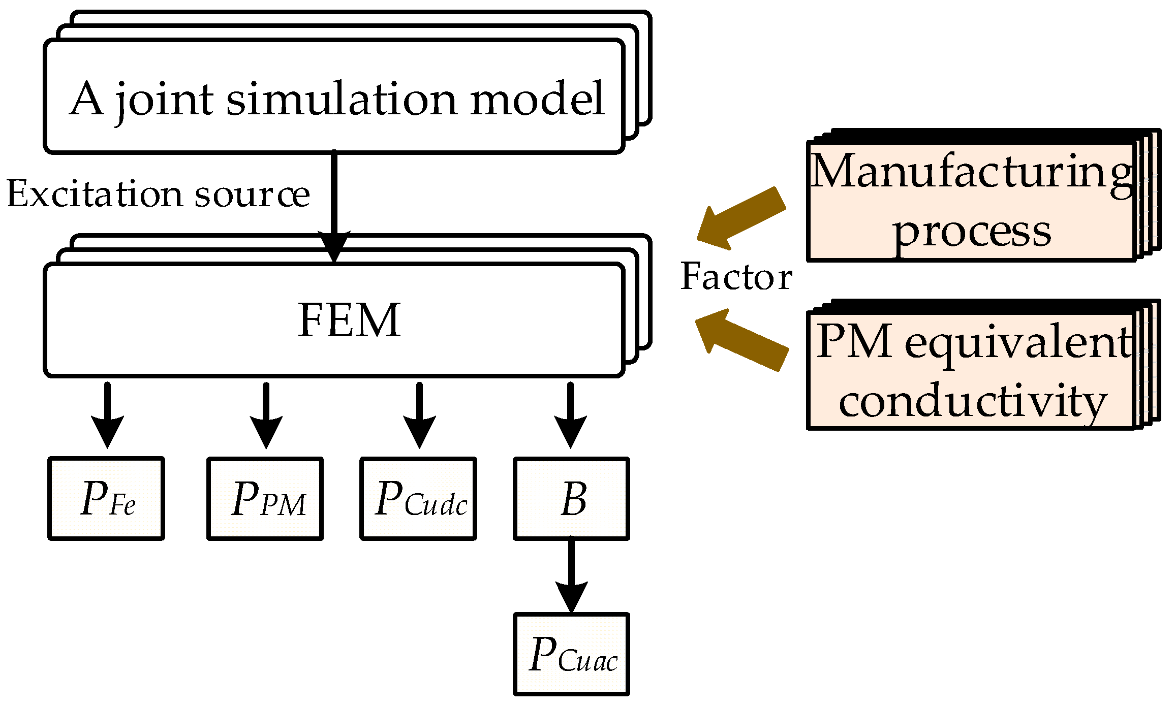
In order to improve the calculation accuracy of losses, factors such as PWM harmonics, processing technology, and segmentation need to be considered, and in order to improve the calculation speed, 2D FEM should be the main modeling basis rather than 3D FEM. Based on this, a calculation scheme as shown in Figure 1 is proposed. Firstly, establish a joint simulation model of motor control and FEM to simulate real excitation sources across the entire operating range. Secondly, inject the excitation source into the 2D finite element model and improve the simulation conditions to consider various external factors that affect the loss calculation. By improving FEM, iron core loss and permanent magnet eddy current loss can be directly calculated. In order to more accurately calculate AC copper loss, it is necessary to calculate AC copper loss through the proposed analytical model based on magnetic field calculation. In summary, the loss values for each motor operating point can be determined. As for mechanical losses, it is difficult to calculate them directly using finite elements. Experimental design will be conducted in the future to establish a mechanical loss calculation model. This paper discusses interior PMSMs because most of the current automotive drive motors on the market are based on this type of motor. However, it does not prevent this method from being used in other permanent magnet motor structures (e.g., surface-mounted PM motors, axial flux designs) because the mechanisms of iron core loss, copper loss, and permanent magnet loss are consistent. At the same time, the joint simulation model also uses the same modeling method, so the overall steps of loss calculation will not change.

A PMSM for electric vehicle drive was used in this study, and its motor performance parameters are shown in

Table 1. PMSM parameters.

Parameters	Value	Parameters	Value
Rated power	70 kW	Poles	8
Rated speed	18,000 rpm	Slots	48
Rated voltage	350 V	Phases	3

. Taking this motor as an example, the modeling method is expounded and demonstrated.

3. The Joint Simulation Model

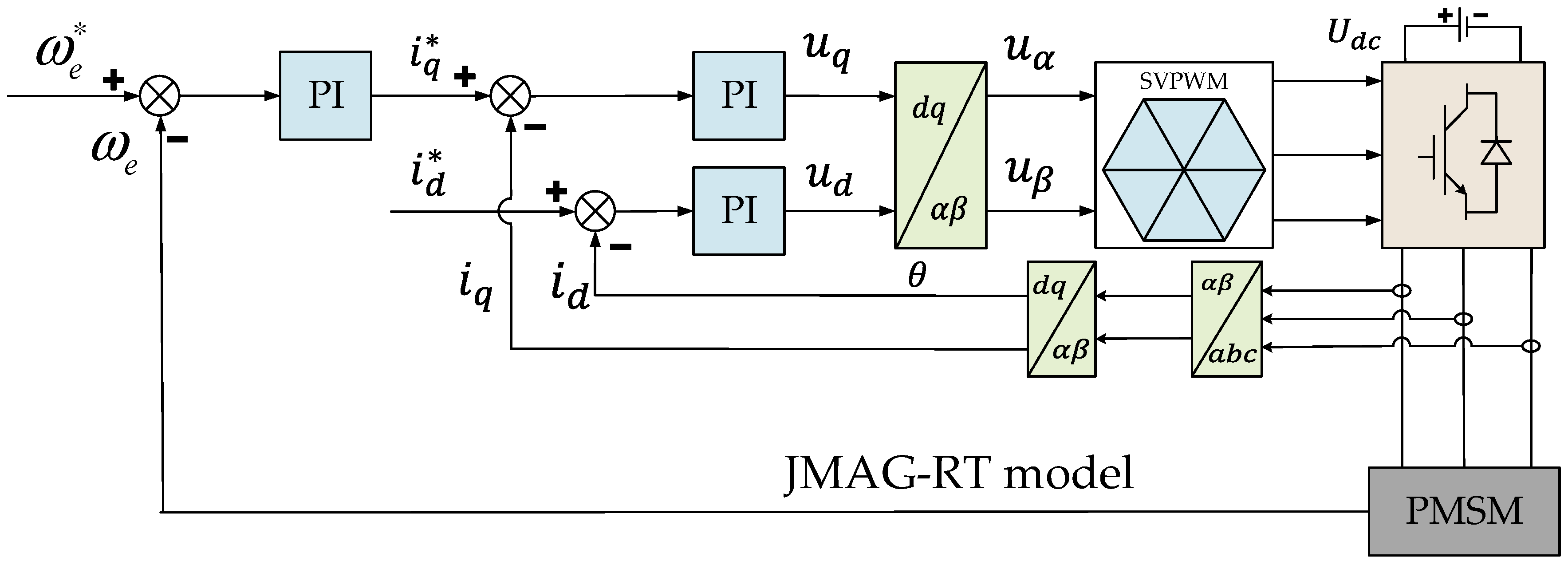
Building a joint model requires simultaneously constructing a PMSM dual loop model and a PMSM finite element model, and coupling them. Direct and rough simultaneous simulation requires too much time due to the difference in time scales. Therefore, it is necessary to use JMAG’s RT (real time) module to reduce the order of the finite element model, and then couple it with the control model, as shown in Figure 2. Among them, the input current, given values i_d* and i_q*, as well as the speed, given value ω_e*, are all derived from vehicle demand and are time-varying parameters.

3.1. Establishment of Motor Control Model

In order to simulate the working conditions of electric vehicle motors more realistically, MTPA (maximum torque per ampere) and field weakening control strategy are chosen to be used. The electromagnetic torque equation and mechanical motion equation of the interior PMSM are as follows:

$$T_e={\displaystyle \frac{3}{2}}{n}_p{i}_q[{\psi }_f+i_d(L_d-L_q)]=T_m+T_r$$

(1)

$$J{\displaystyle \frac{d{\omega }_m}{dt}}=T_e-T_L-B{\omega }_m$$

(2)

where T_m is the excitation torque, T_r is the reluctance torque, n_p is the number of pole pairs, i_d and i_q are the currents of the dq-axes, respectively, L_d and L_q are inductors of dq-axes, respectively, B is the coefficient of viscous friction, and ω_m is the mechanical angular velocity.

3.2. Establishment of Motor RT Model

JMAG-RT is a high-performance real-time simulation tool developed on the JMAG finite element analysis platform, specifically designed for hardware-in-the-loop testing and rapid control prototyping of electric machines, sensors, and power electronics systems. By extracting reduced-order models with high fidelity, this tool translates complex electromagnetic field simulation results into computationally efficient mathematical models executable in real time, while preserving the original numerical accuracy of JMAG. Its key strengths lie in multi-platform deployment support and seamless integration with mainstream control design software such as MATLAB/Simulink 2022 and LabVIEW 2024. These features enable engineers to validate control algorithms, optimize system performance, and accelerate product development cycles within virtual environments.

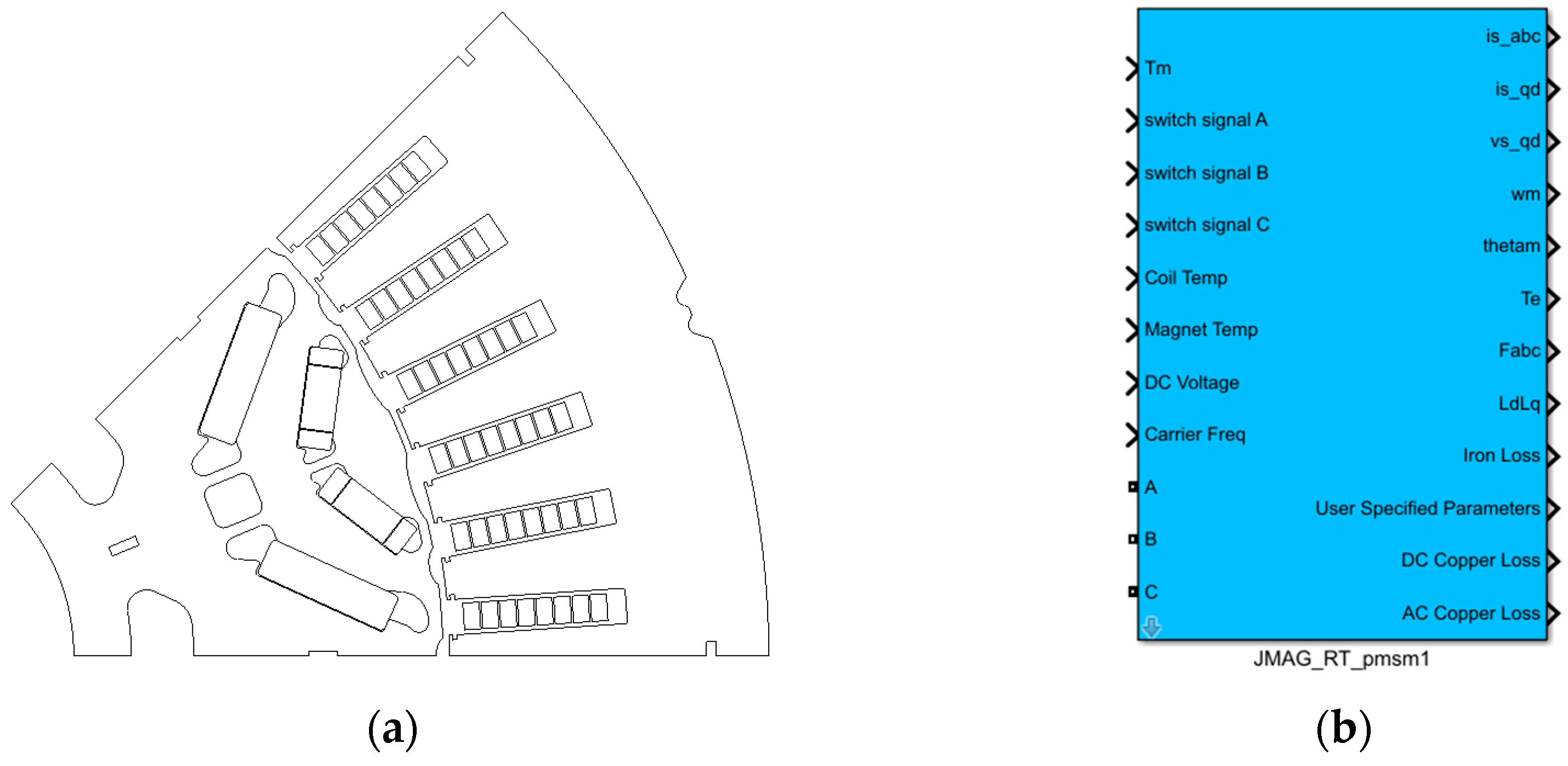
Firstly, a finite element model of the motor in Table 1 was established on the JMAG platform, as shown in Figure 3a. Secondly, batch simulation is conducted based on the actual operating range of the motor, and it is extracted as a reduced-order model of RT through data-driven methods, as shown in Figure 3b. The RT model replaces conventional motor mathematical models, which can consider nonlinear internal factors to improve accuracy, and can be faster than directly coupling finite element models. It is an excellent solution for system simulation.

4. High-Precision Loss Calculation Model

This chapter models and calculates the iron core loss, winding copper loss, and permanent magnet eddy current loss separately, in order to achieve fast and accurate calculation of motor energy consumption.

4.1. Establishment of Iron Core Loss Model

Due to the use of finite element simulation based on PWM excitation in this study, the iron core loss part mainly focuses on material properties, especially considering process improvement calculations. Usually, silicon steel sheets need to go through processes such as shearing and welding, which are also the two main processes considered in this paper.

4.1.1. Cutting Process

In the industrial production process of electric vehicle drive motors, electrical steel plates are generally made into laminations of different sizes and shapes by stamping. However, laser cutting, wire cutting, water cutting, and other methods are also used in small-scale production and laboratory production to cut the iron core laminations into corresponding shapes. In the above processing, different processing methods will generate unacceptable residual stresses at the edges of the iron core laminations, and cause plastic deformation at the cutting surface edges of the iron core laminations, resulting in changes in the microstructure of the material and a decrease in magnetic conductivity and an increase in iron loss at the cutting edges.

In order to consider the influence of the shear process in finite element calculation, it is necessary to simulate the phenomenon of decreased magnetic conductivity caused by the shear process at the cutting edge. Therefore, it is necessary to set a certain depth of degraded area at the edge of the silicon steel sheet, as shown in Figure 4. By adjusting the magnetic permeability and hysteresis loss correction coefficients, the changes caused by the shear process can be simulated, resulting in more accurate calculations of both the magnetic field and losses.

4.1.2. Welding Process

Under the action of an alternating magnetic field, eddy currents will be formed inside the conductor, and the lower the resistance of the conductor, the greater the eddy current loss. To reduce eddy current losses in the stator core of a motor, the stator core is often made of thin electrical steel stacked together. The surface of the electrical steel is coated with insulation to prevent eddy currents from penetrating between the sheets. On the one hand, loose electrical steel laminations need to be connected using connection technology to ensure the strength of the motor stator core. On the other hand, the connection process can damage the insulation coating on the surface of the electrical steel sheet, allowing eddy currents to pass between the sheets and increasing eddy current losses. In the welded electrical steel laminated structure, the insulation coating in the weld area is damaged, and eddy currents can pass through the weld area to form a circuit in the motor stator core, causing an increase in eddy current losses.

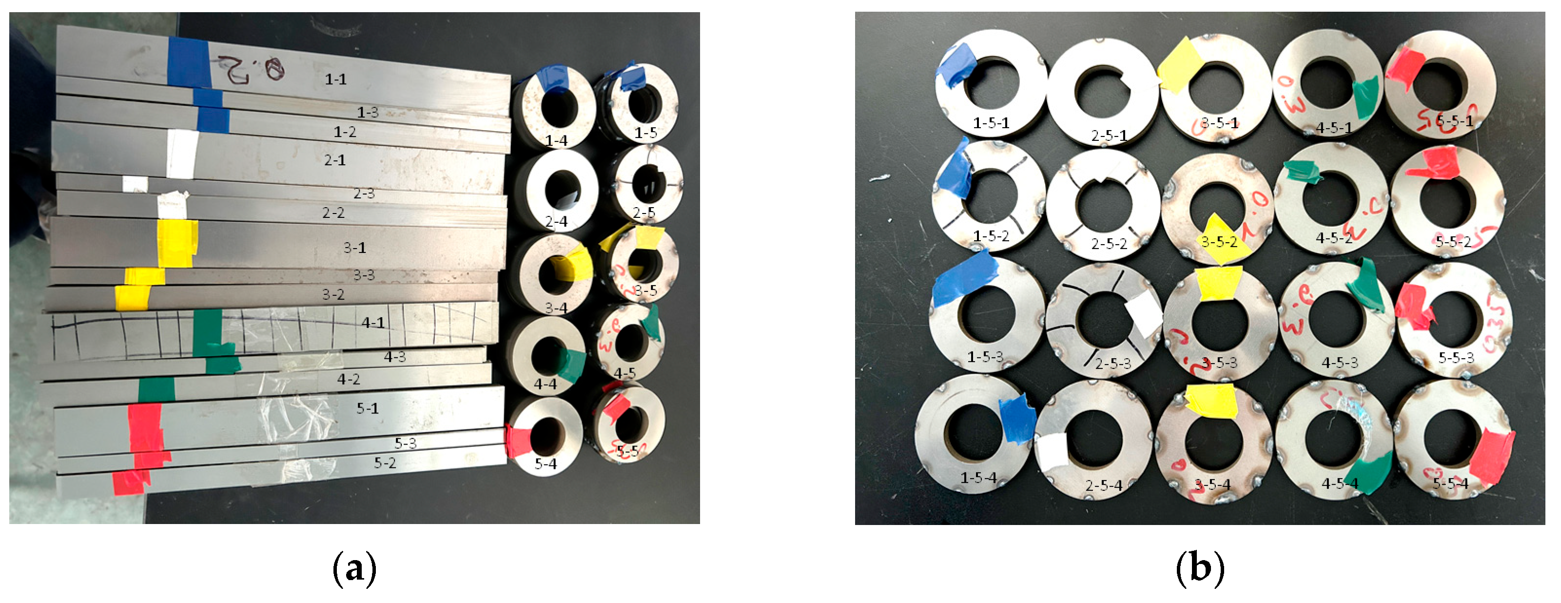
Considering that the FEM is difficult to simulate the additional eddy current circuit caused by welding, unless each silicon steel sheet is finely modeled, which is very time-consuming and difficult to achieve, the changes caused by welding can be taken into account in the characteristics of the material itself to consider its impact on iron loss. Therefore, tests were conducted on various types of welded silicon steel sheets, as shown in Figure 5, to obtain their B-H curves at different frequencies and magnetic flux amplitudes, in order to obtain the B-P curve. Due to the fact that automotive drive motors usually use 10 kHz as the switching frequency in control, selecting 20 kHz as the testing range for silicon steel sheet loss basically includes a relatively large proportion of components, which is sufficient to support the calculation of iron core loss.

For square samples, with a length of 300 mm and widths of 30 mm, 15 mm, and 10 mm, Epstein square rings can be formed by stacking, where 300 mm × 30 mm is the standard size. For circular samples, with an inner diameter of 30 mm and an outer diameter of 60 mm, they can be stacked and tested by winding the wire. The above samples were all obtained using wire cutting technology, which has high machining accuracy and almost no burrs or processing marks left. It also hardly causes a decrease in magnetic permeability and an increase in losses. To simulate the connection method of the motor iron core, the annular sample was welded to consider the influence of the connection process on it, as shown in Figure 5b. For each type of sample, there are four welding forms, namely 2-weld, 4-weld, 6-weld, and 8-weld.

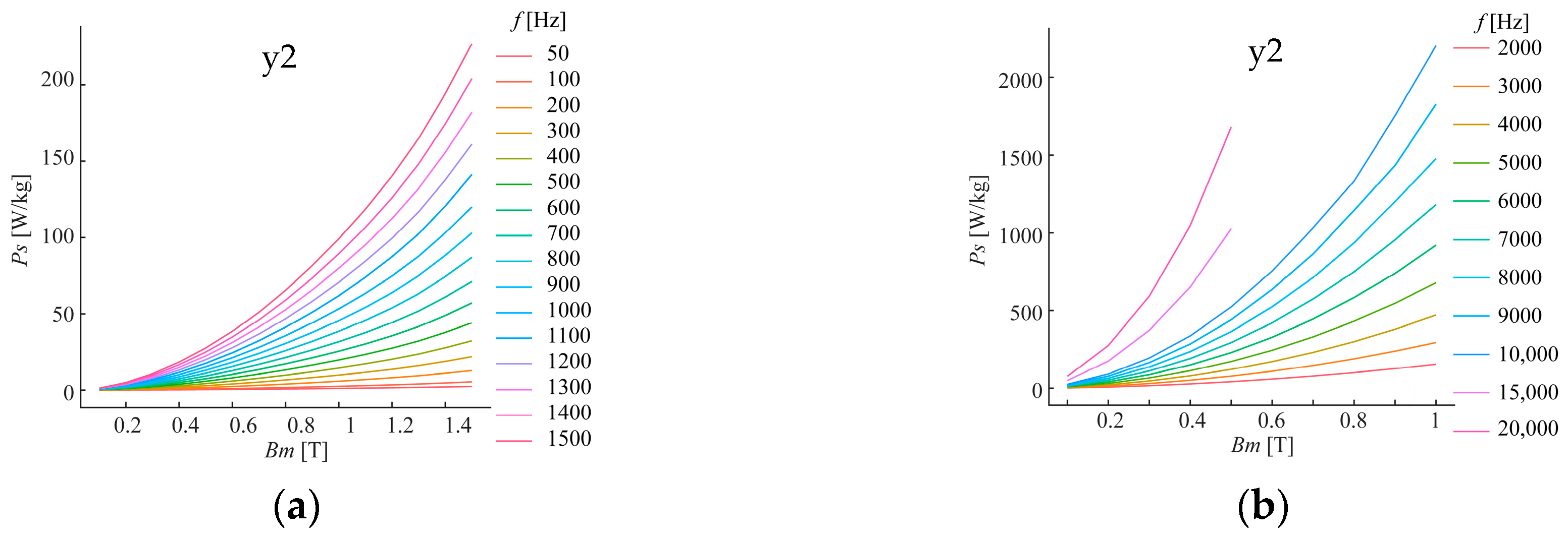
The test results of the circular sample with welding beads are shown in Figure 6, and the loss test results of the circular sample are significantly higher than those of the Epstein square ring. Welding will further increase the specific loss. Another conclusion is that the thicker the silicon steel sheet, the greater the loss. And the more weld beads there are, the greater the iron core loss.

With a more realistic B-P curve for testing, it can be imported into the finite element model to consider the impact of the manufacturing process on iron loss.

4.2. Establishment of Winding Copper Loss Model

Flat wire conductors have low DC resistance, but prominent eddy current effects and high AC copper consumption. As the motor speed increases, the AC effect becomes more significant. In the research process of this paper, the 2D FEM with PWM excitation is still used as the basis, so that the DC copper loss and AC copper loss of the effective section of the conductor can be accurately calculated, and the dimension lacks the DC copper loss and AC copper loss of the end winding.

The traditional method for calculating the losses caused by the end winding is usually to use the following equation for a simple equivalent solution:

$$P_{\mathrm{AC}}=I^2·R·k$$

(3)

$$k={\displaystyle \frac{1}{2}}\gamma {\displaystyle \frac{\sinh \gamma +\sin \gamma }{\cosh \gamma -\cos \gamma }}$$

(4)

$$\gamma ={\displaystyle \frac{b}{\delta }}$$

(5)

where P_AC is the conductor loss considering the skin effect, δ is the skin depth, b is the length of the short side of the rectangular conductor cross-section, generally guiding the thickness of the body, k is the coefficient of resistance increase caused by the skin effect, R is the equivalent resistance value of the winding, and I is the effective current value. When the current contains high-order harmonics, Fourier decomposition is performed to solve them by superposition.

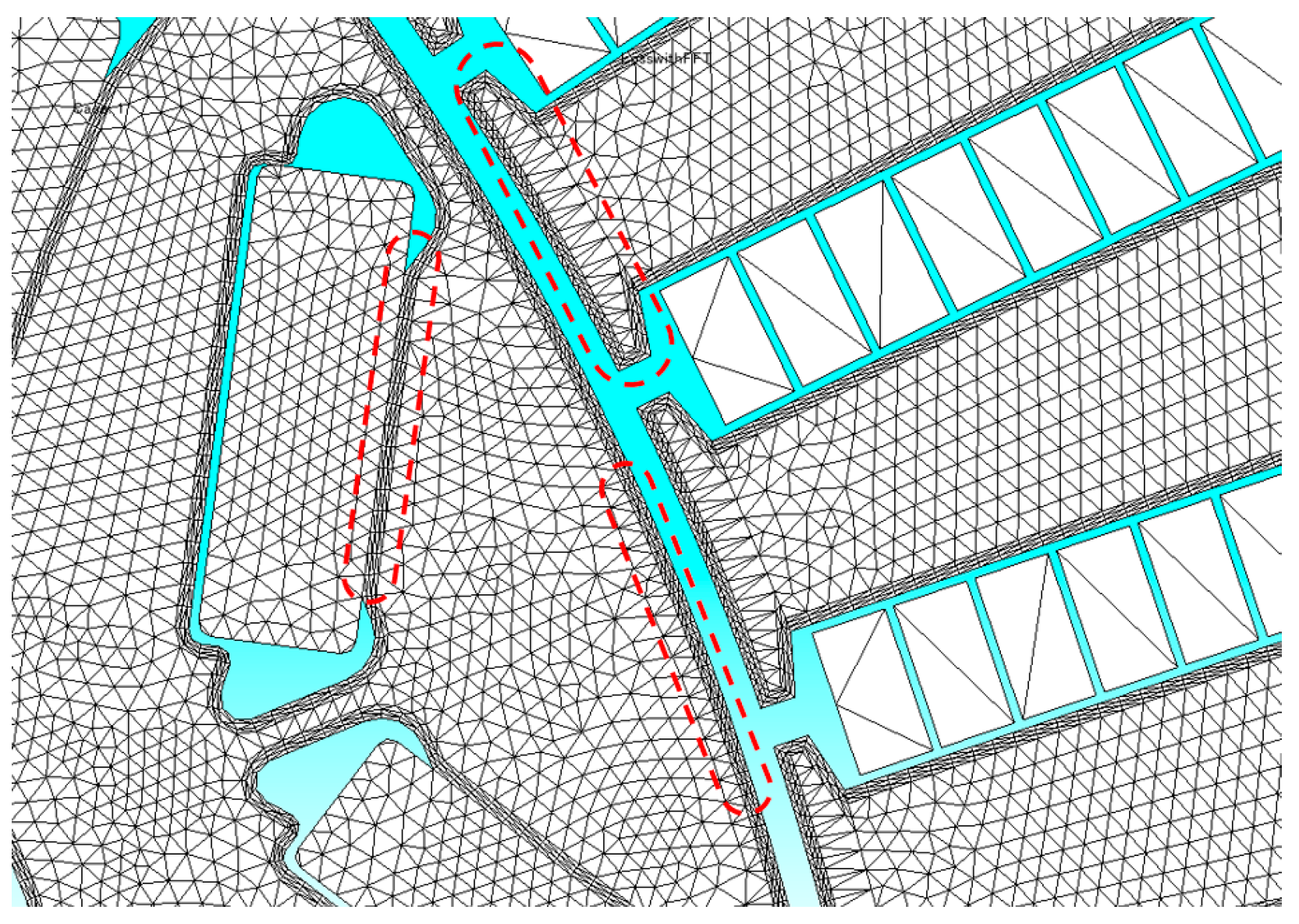
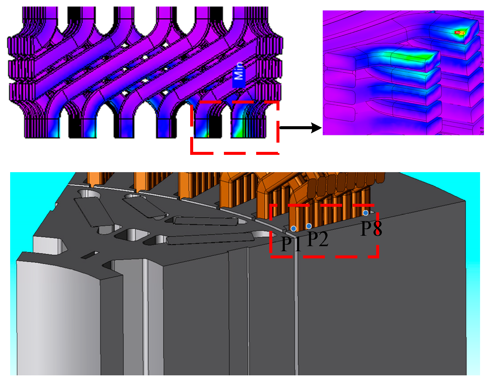
This analytical method only considers the influence of skin effect on conductor loss, ignores the effect of proximity between conductors, and also ignores the influence of axial leakage flux of the motor on loss. Figure 7 shows the distribution cloud map of end winding losses in the three-dimensional finite element model. The conductor near the iron core has a greater proportion of losses due to the influence of motor leakage, and the impact of motor leakage on winding losses cannot be ignored.

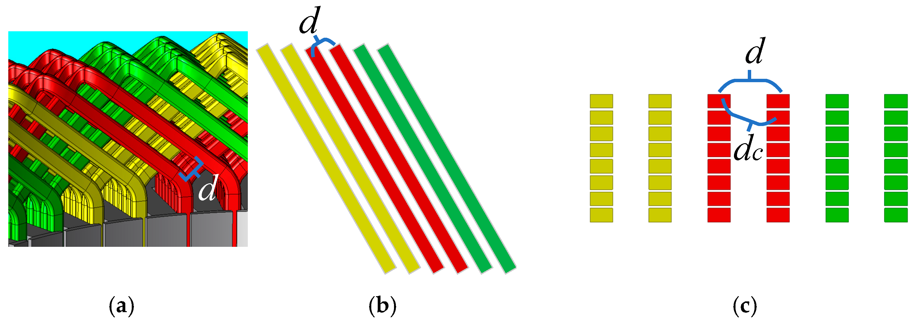
For the additional losses caused by alternating current passing between end conductors that are not affected by magnetic leakage, both skin effect and proximity effect must be considered simultaneously. For this purpose, this paper adopts a straight conductor model after the end winding is stretched, and establishes a 2D model based on it to achieve approximate equivalence of the end, as shown in Figure 8. The lateral spacing d of the equivalent model is consistent with the parallel spacing of the end conductors, and the longitudinal spacing is the interlayer distance of the conductors. Solve for the magnetic field generated by the conductor. According to Ampere’s Loop Law, the magnetic field B generated by a wire with an effective current I at a distance of d_c from another conductor in space is as follows:

$$B={\displaystyle \frac{{\mu }_{0}I}{2\pi d_{\mathrm{c}}}}$$

(6)

where μ₀ is the vacuum magnetic permeability.

The vector superposition of the magnetic fields generated by each conductor is used to obtain the magnetic field generated by the end winding. After completing the process of solving the magnetic field, combined with the analytical formula for eddy current loss, the formula for solving the end loss P_end is as follows:

$$P_{\mathrm{end}}=I^2·R·k+{\displaystyle \frac{{\pi }^2}{3}}{f}^2\sigma a^{3}b{l}_{\mathrm{end}}{B}_{\mathrm{rm}}^2{\cos }^2(\omega t){\eta }_{\mathrm{rd}}^2+{\displaystyle \frac{{\pi }^2}{3}}{f}^2\sigma a{b}^3{l}_{\mathrm{end}}{B}_{\mathrm{tm}}^2{\cos }^2(\omega t){\eta }_{\mathrm{td}}^2$$

(7)

where a, b, and l_end represent the width, thickness, and equivalent length, respectively, of the flat wire conductor after the end winding is stretched. B_m is the amplitude of the fundamental magnetic flux density, B_rm and B_tm represent the radial and tangential magnetic flux density amplitudes, respectively, σ is the conductivity, f is the frequency of magnetic field variation, and ω is the fundamental angular frequency of the magnetic field. In addition, for non-sinusoidal magnetic fields, the introduction of the magnetic field distortion coefficient η_d considers the influence of high-order harmonics, where η_rd and η_td are the magnetic field distortion coefficients in two directions, respectively.

4.3. Establishment of Permanent Magnet Eddy Current Loss Model

In an ideal state, the magnetic field in the air gap of a PMSM is distributed in a pure sine shape and has the same rotational speed as the rotor. Therefore, the magnetic field in the rotor magnet and air gap is relatively static, and there is no eddy current loss in the rotor. However, due to the abundant harmonics in the air gap, the harmonic speed cannot rotate synchronously with the motor, resulting in eddy current losses on the permanent magnet. Due to the volume limitation of PMSMs used in electric vehicles, a large number of spatial harmonics generated by uneven distribution of motor windings can also generate significant eddy current losses in the rotor magnetic steel. In summary, due to the inclusion of various spatial and temporal harmonic components in the air gap magnetic field, most of these harmonic components are caused by the non-sinusoidal distribution of stator magnetic potential, stator cogging effect (uneven air gap magnetic conductivity caused by motor core slotting), and non-sinusoidal stator phase current. The harmonic components of the air gap magnetic field generate induced electromotive force on the rotor magnet due to relative motion with the rotor, resulting in eddy current losses. In other words, the eddy current losses inside the magnetic steel are caused by harmonic magnetic fields.

Accurate calculation of internal losses in permanent magnets often requires the use of 3D FEM for calculation. By constraining the total surface current on the cross-section of each permanent magnet to 0, the 2D FEM can be approximately used to calculate the eddy current loss of the permanent magnet. When the axial length of the permanent magnet is much greater than the width, this method can achieve good approximation results, but when the axial length of the permanent magnet is short or there are axial segments, it will produce significant calculation errors. Moreover, when considering the eddy current losses caused by PWM harmonics, the FEM calculation time is often difficult to accept, and an efficient and high-precision permanent magnet eddy current loss calculation model is urgently needed.

According to the derivation, the expression for permanent magnet eddy current loss is [22] as follows:

$$P_{2D}={\displaystyle \frac{B_{av}^2}{{\xi }_r^2+{\xi }_i^2}}{\displaystyle \frac{4b_{PM}·d_{PM}·\sigma ·{\omega }^2}{a_{PM}}}\times {\displaystyle \sum _{n=1,3,5,7\dots }1/({(n\pi /a_{PM})}^4+{(\omega \mu \sigma )}^2)}$$

(8)

$$\begin{array}{cc}\hfill P_{3D}& ={\displaystyle \frac{N_s\times 32B_{av}^2}{{\xi }_r^2+{\xi }_i^2}}·{\pi }^2·a_{PM}·b_{PM}·d_{PM}·\sigma ·{\omega }^2\hfill \\ & \times {\displaystyle \sum _{n=1,3,5\dots }{\displaystyle \sum _{m=1,3,5\dots }1/({({(n\pi /a_{PM})}^2+{(m\pi /b_{PM})}^2)}^2+{(\omega \mu \sigma )}^2)}}\hfill \\ & \times (1/{(b_{PM}·n)}^2+1/{(a_{PM}·m)}^2)\hfill \end{array}$$

(9)

where a_PM, b_PM, and d_PM are the width, axial length, and thickness, respectively, of the permanent magnet, ω is the angular frequency, μ is the magnetic permeability of the permanent magnet, and N_s is the number of axial segments. And ξ_r and ξ_i are the real and imaginary parts, respectively, of the parameter ξ used to reflect the strength of the eddy current effect in permanent magnets. The calculation method is as follows:

$${\xi }_{2Dr}+j{\xi }_{2Di}=1-{\displaystyle \frac{j\omega \mu \sigma }{{\pi }^2}}\times {\displaystyle \sum _{n=1,3,5\dots }8/n^2/({(n\pi /a)}^2+j\omega \mu \sigma )}$$

(10)

$${\xi }_{3Dr}+j{\xi }_{3Di}=1-{\displaystyle \frac{64}{{\pi }^4}}·j\omega \mu \sigma \times {\displaystyle \sum _{n=1,3,5\dots }{\displaystyle \sum _{m=1,3,5\dots }1/{(mn)}^2/({(n\pi /a)}^2+{(m\pi /b)}^2+j\omega \mu \sigma )}}$$

(11)

In order to make 2D FEM more accurately equivalent to 3D FEM, it means making ξ_2D equal to ξ_3D, it is necessary to find the optimal σ_mod such that

$$\min ({\xi }_{2D}-{\xi }_{3D})=\min ({\xi }_e^r+j{\xi }_e^i)=\sqrt{{({\xi }_e^r)}^2+{({\xi }_e^i)}^2}$$

(12)

According to Equations (10) and (11), it can be seen that the conductivity correction is related to the geometric dimensions of the permanent magnet and the frequency of the electrical excitation. Compared with the traditional method of equivalent based only on the size of the permanent magnet, it considers more the influence of frequency and is more accurate. Secondly, if segmented equivalence needs to be considered, simply substitute the geometric dimensions of the permanent magnet for each segment.

5. Simulation and Experimental Verification

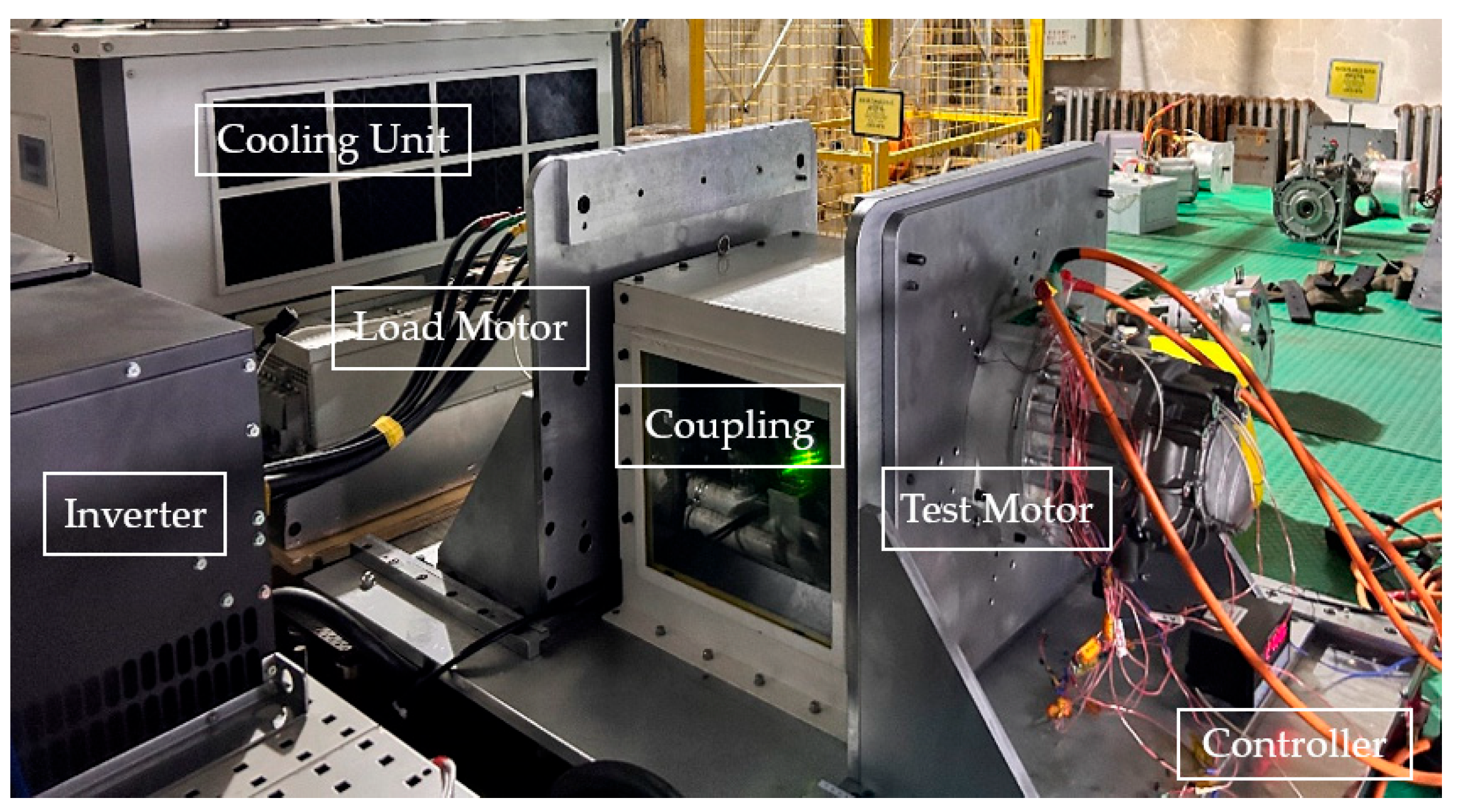
In order to verify the effectiveness of the proposed calculation method, an experimental platform was built as shown in Figure 9. The tested motor is connected to the load motor through a transmission shaft, with a torque sensor inserted in between for measuring torque and speed. The DC power supply supplies power to the tested motor through an inverter and is connected to a power analyzer for testing its current, voltage, and electrical power. The entire experiment was conducted at room temperature, using a water-cooled device to control the temperature of the motor. At the same time, a torque sensor HBM T40B was used to collect torque values in real time with an accuracy of one thousandth. In addition, use a power analyzer to record the power values of the motor under different operating conditions, with a sampling frequency of 20 Hz.

Among them, the parameters of the test prototype are shown in Table 1, and in order to meet the special requirements of different loss verifications, multiple functional prototypes were customized and modified based on this prototype, as shown in

Table 2. Prototype preparation and description.

	Winding	Iron Core Technology	Permanent Magnet	For
1	Flat wire	Welding	√	Basics
2	Litz wire	Welding	√	Copper loss
3	Flat wire	Cutting	√	Iron core loss
4	Flat wire	Welding	×	Mechanical loss

. Prototypes −1, −2, −3, and −4 are all motors of the same model. The number of conductors per slot and the number of parallel branches in the Litz wire winding of prototype 2 and the flat wire winding of prototype 1 need to be equal, in order to better verify the calculation results of AC copper loss. Prototype 3 is used to compare the effects of cutting and welding processes on iron loss. The permanent magnets of Prototype 4 are not magnetized to eliminate the influence of magnetic reluctance torque on mechanical loss testing, and other aspects are consistent with Prototype 1.

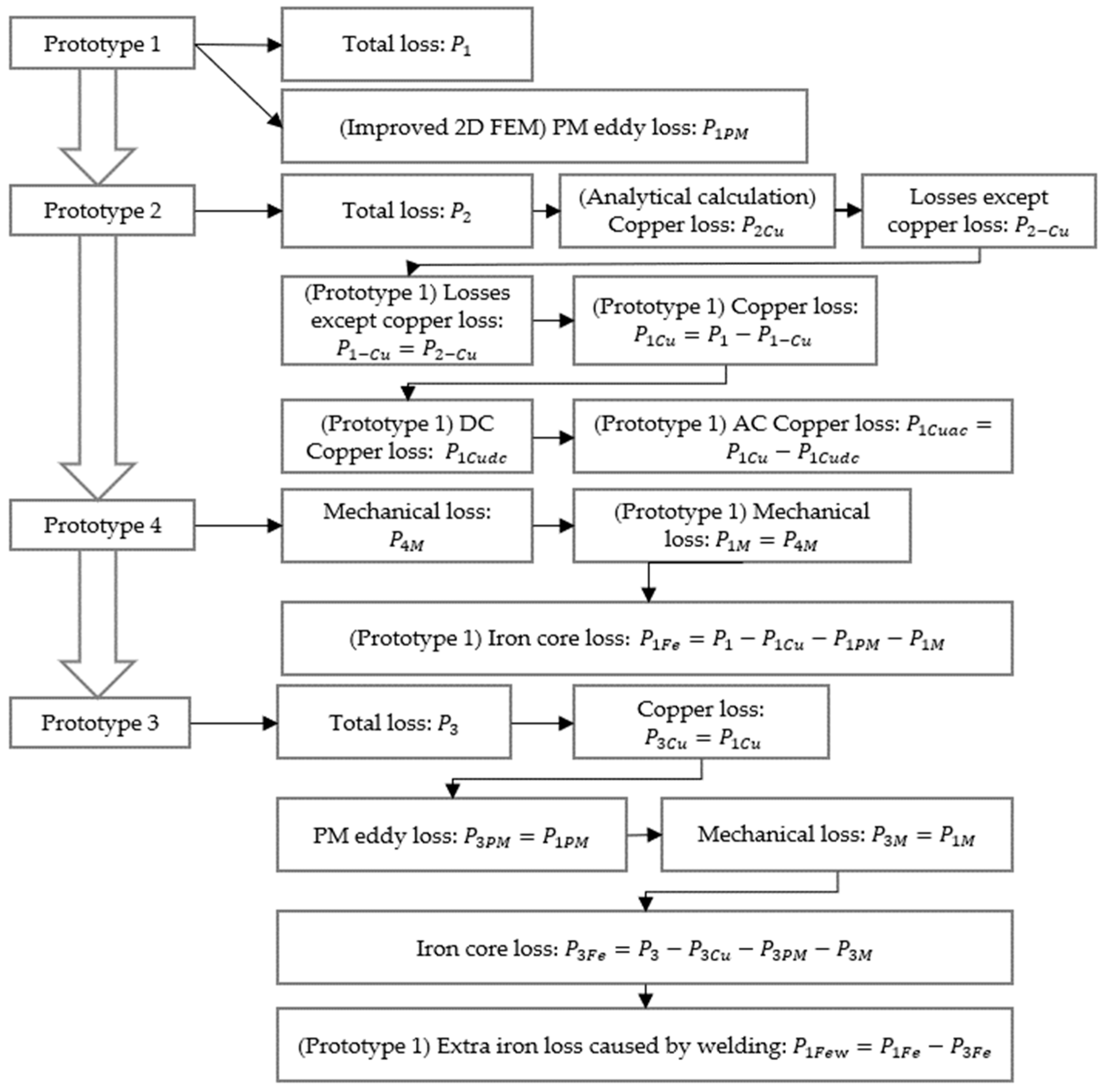
The process of separating losses at each operating point is shown in Figure 10. Prototype 1 is the focus of attention, and after each step in Figure 10, the permanent magnet eddy loss, mechanical loss, copper loss (including total copper loss, DC copper loss, and AC copper loss), and iron loss (including total iron loss and additional iron loss caused by welding) of Prototype 1 will be obtained.

5.1. Verification of PWM Harmonic Current Simulation

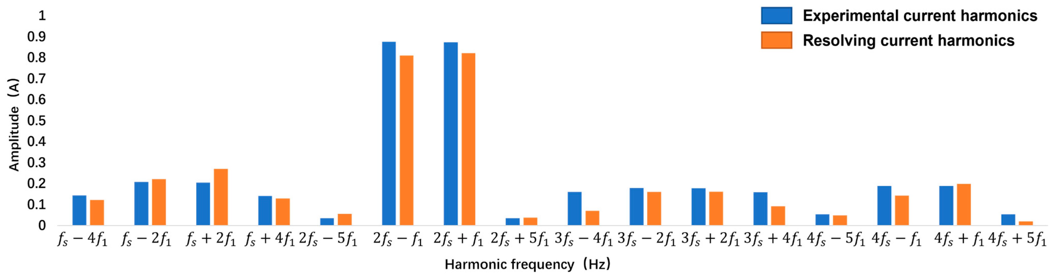
The simulation of high-precision excitation is the foundation and guarantee for accurate loss simulation calculation. Therefore, the accuracy of the output excitation of the joint simulation model needs to be verified first. The studies were performed on an experimental setup employing a three-phase two-level voltage source inverter with SVPWM (space vector PWM) and rotor-flux-oriented vector control strategy.

FFT processing was performed on the experimental currents at switching frequencies of 1000 rpm, 27 Nm, and 10 kHz, and compared with the currents obtained from the joint simulation. The frequency domain results are shown in Figure 11.

Due to the fact that the main factor affecting losses is the switching sub sideband harmonics [23], the key sideband harmonic amplitudes at frequencies f_s ± k_ef₁, 2f_s ± k_of₁, 3f_s ± k_ef₁, and 4f_s ± k_of₁ (k_e = 2, 4…, k_o = 1, 5…) are compared in detail. From the above results, it can be seen that the harmonic amplitude values of the key secondary sidebands are basically consistent, which proves the accuracy of the joint model for current source excitation simulation and lays the foundation for subsequent finite element simulation.

5.2. Verification of Loss Model

According to the loss separation scheme shown in Figure 9, the calculation accuracies of copper loss, permanent magnet eddy loss, mechanical loss, and iron core loss were verified, respectively.

5.2.1. Winding Copper Loss Model

In order to verify the calculation accuracy of copper loss, especially to measure the value of AC copper loss, copper loss separation was carried out based on Prototype 1 and Prototype 2. The specific steps are shown in Figure 9. Due to the small cross-sectional area of litz wire, the copper loss P_2Cu of prototype 2 can be regarded as only including DC copper loss. In this way, the AC copper loss of Prototype 1 can be obtained by making a difference and verified while ensuring that other losses of Prototype 1 and Prototype 2 are consistent. The DC copper losses of the two prototypes are as follows:

$$P_{2Cu}=3I^2{R}_2$$

(13)

$$P_{1Cudc}=3I^2{R}_1$$

(14)

Apart from the copper loss, the other losses of the two prototypes are the same:

$$P_{2-Cu}=P_2-P_{2Cu}=P_{1-Cu}=P_1-P_{1Cu}$$

(15)

where P₁ and P₂ are the total losses of Prototype 1 and Prototype 2, respectively. Therefore, through the test of the two prototypes, the calculation mode of the AC copper loss of prototype 1 can be obtained as follows:

$$\begin{array}{cc}\hfill P_{1Cuac}& =P_1-P_{1-Cu}-P_{1Cudc}\hfill \\ & =P_1-P_{1Cudc}-(P_2-P_{2Cu})\hfill \end{array}$$

(16)

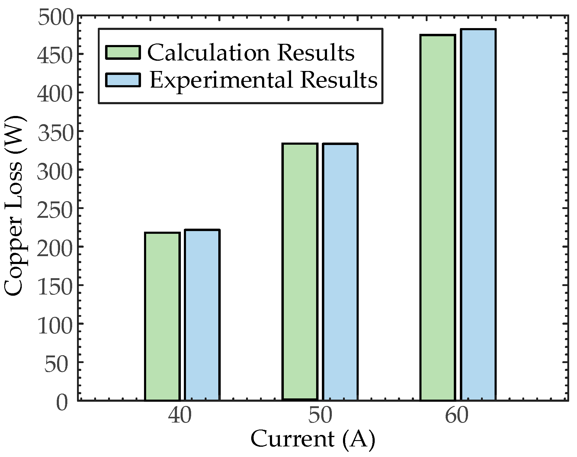
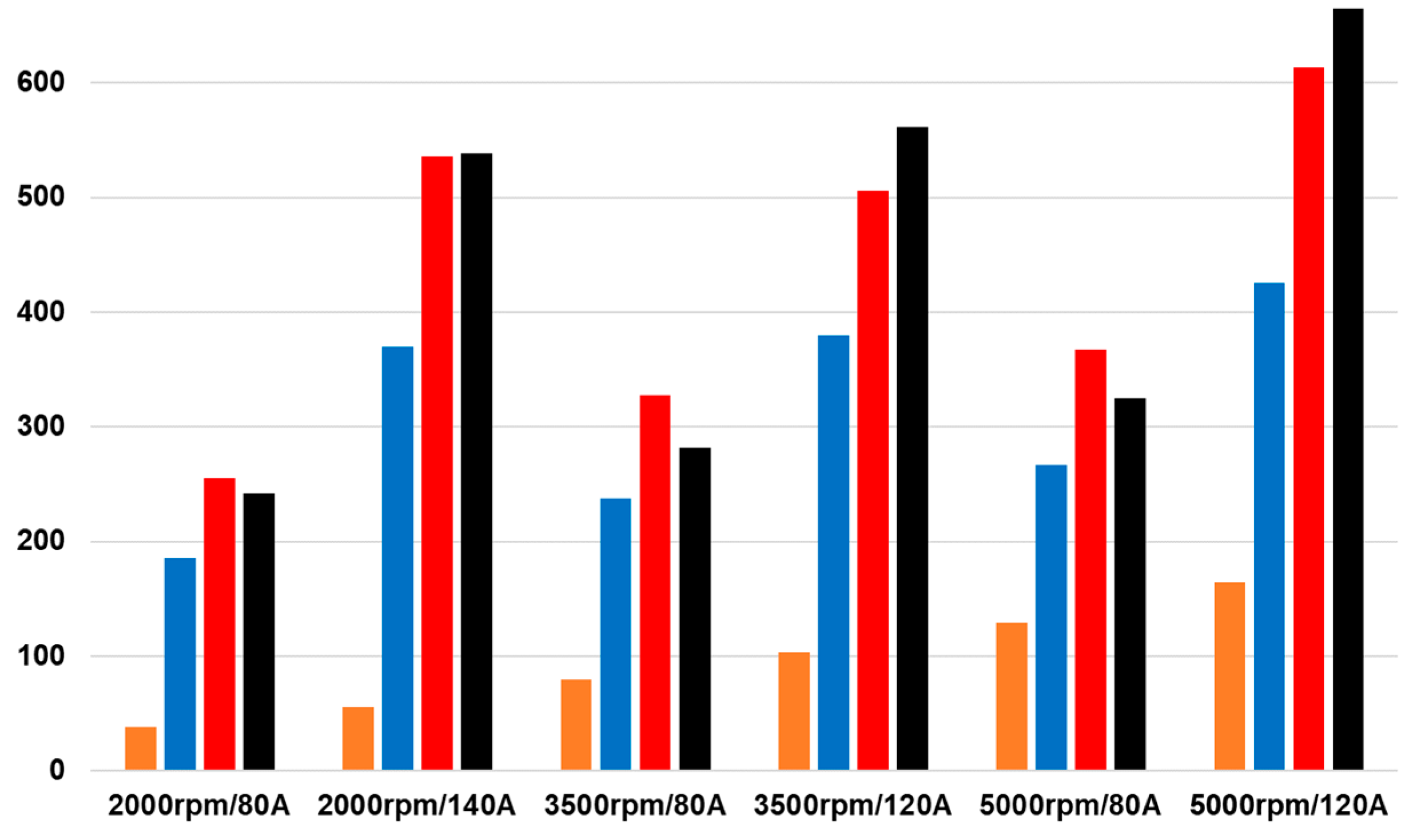
Figure 12 shows the copper loss calculated by the proposed copper loss calculation model at a speed of 4000 rpm under different current conditions, as well as the comparison with the experimental separation loss. The calculated results are consistent with the experimental separation results, which verifies the proposed method in this paper.

Table 3. Verification results of Litz wire motor and flat wire motor.

Current	Flat Wire Prototype Efficiency	Litz Wire Prototype Efficiency	Calculation Results	Experimental Results
40 A	93.38%	91.92%	200.45 W	196.03 W
50 A	94.16%	91.83%	309.12 W	293.30 W
60 A	93.51%	91.10%	454.33 W	464.49 W
70 A	93.63%	90.76%	611.46 W	591.73 W
80 A	91.01%	89.99%	806.96 W	805.85 W

takes 3000 rpm as an example to record in detail the efficiency of the flat wire and litz wire prototypes under different amplitude current operating points, as well as the comparison between the separated flat wire winding loss results and the calculated results.

The overall error between the experimental separation loss and the calculated flat wire loss remains within 40 W. The deviation between the measured separation results and the semi-analytical results at most operating points is less than 8%, and the deviation is less than 4% at operating points with larger current values. At low current operating points, due to the small output power of the prototype and the relatively small copper loss value, the relative error of the same loss difference in the low-loss operating range is relatively large, about 10~20%.

5.2.2. Permanent Magnet Eddy Current Loss Model

Three-dimensional FEM is considered to be able to accurately calculate the permanent magnet eddy current loss. Therefore, this paper will compare the improved 2D FEM results with the 3D FEM results to verify the accuracy of permanent magnet eddy current loss calculation.

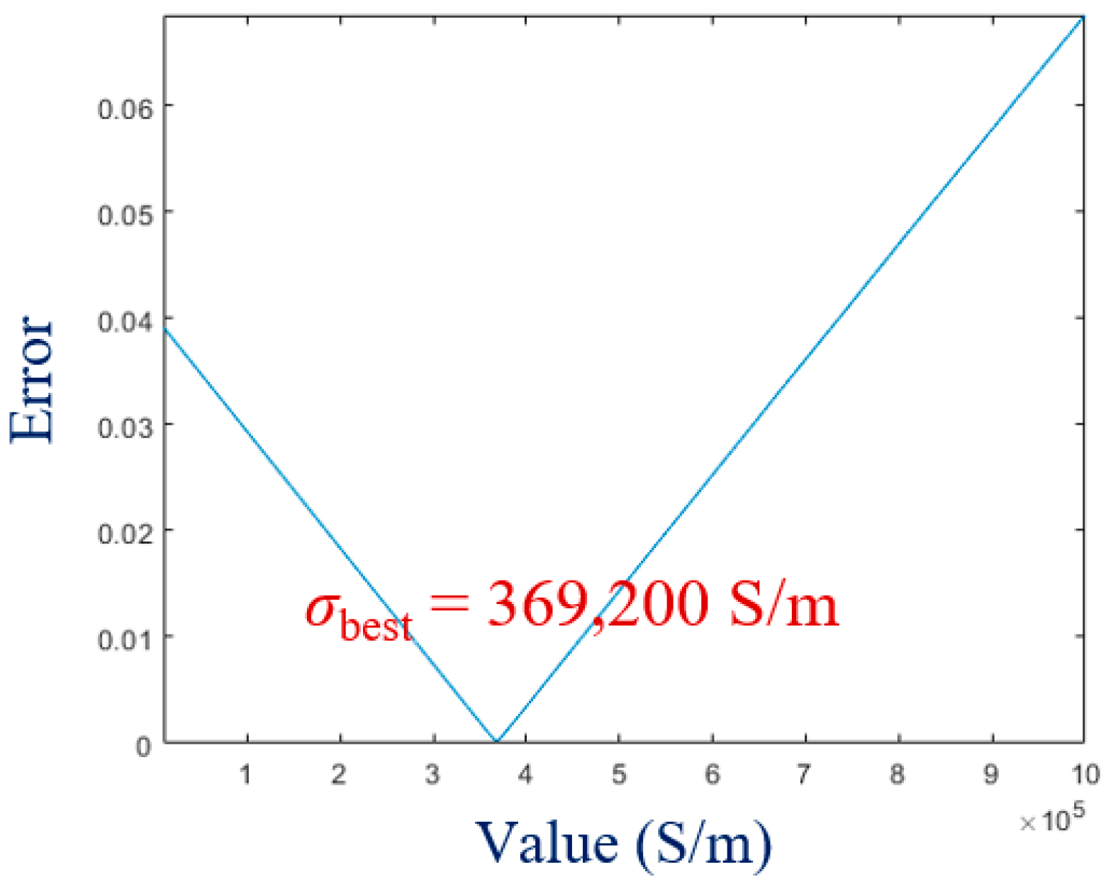
Under the working conditions (1500 rpm@50 A), simulations were conducted using both 2D FEM and 3D FEM. According to Equation (12), the conductivity correction results of the permanent magnet material in 2D FEM are shown in Figure 13.

When the conductivity σ_mod = 369,200 S/m, the error between ξ_2D and ξ_3D is minimized, and this value is the corrected conductivity. Substituting it into 2D FEM, the following results are obtained, as shown in

Table 4. Verification results of permanent magnet eddy current loss.

Condition	2D FEM (Before Correction)	2D FEM (After Correction)	3D FEM
1500 rpm@50 A	7.8443 W	4.1734 W	3.5111 W
3000 rpm@50 A	27.8054 W	14.5004 W	12.9264 W

. It can be observed that after correcting the conductivity of the permanent magnet, the 2D and 3D simulation results are very close, further verifying the effectiveness of this correction method.

To verify the segmentation factor, a segmented 3D FEM was also established at 1500 rpm, and the equivalent conductivity was calculated based on Equation (12) to be 170,500 S/m. After incorporating the 2D FEM, the results are shown in

Table 5. Calculation results of permanent magnet eddy current loss of segmented motor model.

Condition	2D FEM (Before Correction)	2D FEM (After Correction)	3D FEM
1500 rpm@50 A	7.8443 W	2.0588 W	1.8041 W

.

5.2.3. Mechanical Loss Test

Mechanical losses are difficult to model and calculate using simulation methods, so it is necessary to calculate them through experimental testing. Install Prototype 4 in Table 2 at the position of the tested motor in Figure 8, control the load motor to the specified speed, and read the torque sensor reading at this time. The absolute value of the product of the torque sensor reading and the speed is the mechanical loss at that speed. Mechanical losses are only related to rotational speed and not to the magnitude of current.

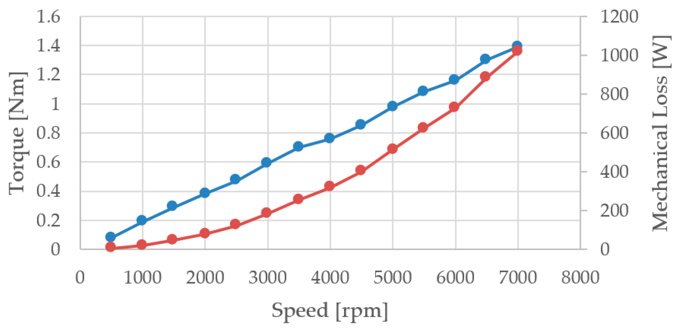
The calculation method for mechanical loss is to multiply the mechanical resistance torque by the rotational speed; that is, the mechanical loss is proportional to the rotational speed. This is obtained by fitting experimental test data, as shown in Figure 14. The red curve represents the relationship between mechanical loss and rotational speed, and the blue curve represents the relationship between mechanical resistance torque and rotational speed. After testing, the resistance torque coefficient was calculated to be 1.96 × 10⁻⁴ Nm/rpm through fitting.

5.2.4. Iron Core Loss Model

It is difficult to directly measure the iron core loss through experiments. Therefore, based on other loss measurements or calculations, an iron loss separation scheme as shown in Figure 9 was designed.

This paper extracted six typical operating points at low, medium, and high speeds for comparative analysis of iron loss. The calculation methods for iron loss are divided into three schemes:

Method-1: considering only the calculation of iron loss under sine current excitation (Sinusoidal excitation).

Method-2: considering the calculation of iron loss under PWM harmonic current excitation.

Method-3: considering both PWM harmonic current excitation and processing technology for iron loss calculation.

Finally, a comparative analysis is conducted with the iron loss separated from the experiment to verify the effectiveness of the iron loss calculation method. The comparison schemes for iron loss are shown in

Table 6. Verification results of iron loss.

Condition	Method-1	Method-2	Method-3	Experimental Results
2000 rpm@80 A	38.4 W	185.86 W	255 W	242.1 W
2000 rpm@140 A	56.2 W	369.63 W	536.1 W	538.6 W
3500 rpm@80 A	79.3 W	237.6 W	327.2 W	281.5 W
3500 rpm@120 A	103.6 W	379.91 W	505.8 W	561.8 W
5000 rpm@80 A	128.6 W	267.01 W	367 W	324.5 W
5000 rpm@120 A	164.6 W	425.52 W	613.7 W	664.6 W

. The comparison chart of iron loss is shown in Figure 15. From the table, it can be seen that compared to the iron loss calculation results under sinusoidal excitation, the iron loss calculation results under PWM harmonic current excitation are closer to the experimental separated iron loss, with a maximum error of about 30% compared to the experimental iron loss. When considering both PWM harmonic current excitation and the iron loss calculation method under processing technology, the iron loss calculation results are closer to the experimental separation iron loss results, with a maximum error of about 15%. At the same time, the percentage of iron loss deviation value to input power is within 0.45%, which basically meets the engineering requirements and verifies the effectiveness of the iron loss calculation method.

5.3. Verification of Motor Efficiency Map

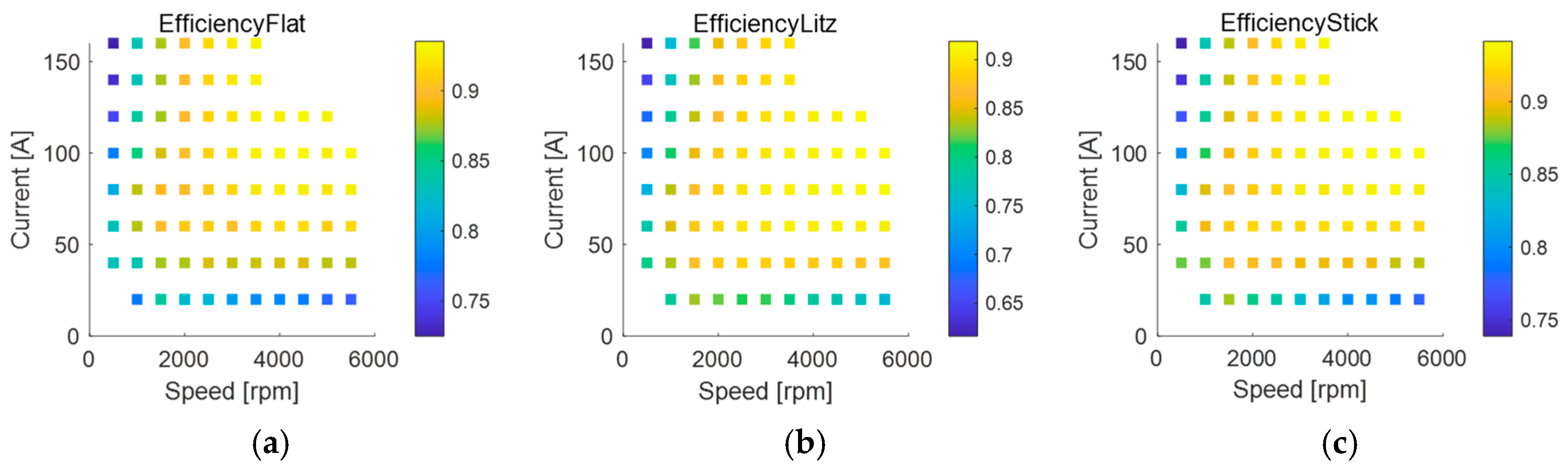
After verifying various loss calculation methods, it is necessary to integrate these models and generalize them for calculation under full speed domain conditions. Firstly, Prototypes 1, 2, and 3 were tested using a power analyzer, and the efficiency distribution of the three motors was obtained as shown in Figure 16. Among them, the efficiency of the cutting core motor is the highest, with a maximum of 94%, as cutting iron cores have lower iron loss, and the maximum efficiency of the flat wire motor is 93.5%. Due to the large DC copper loss, the Leeds line motor has the lowest efficiency, with a maximum of 92%.

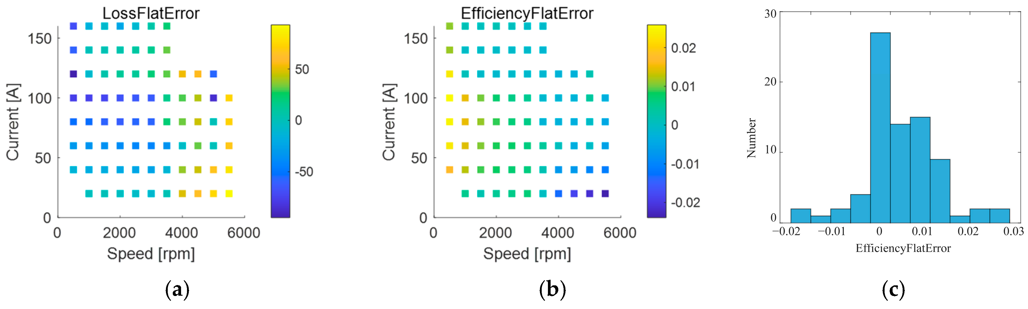
By calculating various loss models, the computational efficiency value of Prototype 1 within the full speed domain was obtained, and an error analysis was conducted with the experimental efficiency, as shown in Figure 17.

The difference between the simulated and tested losses of the flat wire motor is shown in Figure 17a. The efficiency error of the flat wire motor simulation is shown in Figure 17b between positive and negative 100 W, and its distribution pattern is shown in histogram 17c. It can be seen that among the 78 operating points, the efficiency calculation error of 70 operating points is within 1.5%.

6. Conclusions

This paper proposed an accurate efficiency calculation method for electric vehicle drive PMSMs within the full speed range of operating conditions. In order to achieve this goal, the research mainly focused on two aspects of work and contributions. Firstly, the research created an RT model based on high-precision FEM, which enables accurate simulation of motor input excitation under different operating conditions during the manufacturing stage. Secondly, separate models were developed for iron loss, copper loss, and permanent magnet eddy current loss. Regarding iron core loss, the research considered PWM current harmonic factors and shear and welding process factors on the basis of traditional 2D FEM, making the calculation of iron core loss more accurate and realistic. A more accurate analytical calculation method has been proposed for copper loss. Based on 2D magnetic field calculations, the AC copper loss of not only the conductors in the slot but also the end conductors has been fully considered, improving the calculation accuracy and speed. The concept of equivalent conductivity is proposed for the eddy current loss of permanent magnets, achieving the effect of equivalent 3D FEM using 2D FEM. At the same time, the axial segmentation factor can be considered to achieve rapid calculation of permanent magnet eddy current loss in the full speed domain. Finally, a loss separation scheme was designed, and the calculation accuracy of the motor’s efficiency over the entire operating range was verified through the integration of various loss models. The efficiency error of the vast majority of operating points was within 1.5%.