Article

Interpretable Machine Learning for High-Accuracy Reservoir Temperature Prediction in Geothermal Energy Systems

by
Mohammadali Ahmadi
Department of Chemical and Petroleum Engineering, Sharif University of Technology (SUT), Tehran P.O. Box 14588-89694, Iran
Energies 2025, 18(13), 3366; https://doi.org/10.3390/en18133366
Submission received: 10 May 2025 / Revised: 9 June 2025 / Accepted: 19 June 2025 / Published: 26 June 2025

Abstract

Accurate prediction of reservoir temperature is critical for optimizing geothermal energy systems, yet the complexity of geothermal data poses significant challenges for traditional modeling approaches. This study conducts a comprehensive comparative analysis of advanced machine learning models, including support vector regression (SVR), random forest (RF), Gaussian process regression (GP), deep neural networks (DNN), and graph neural networks (GNN), to evaluate their predictive performance for reservoir temperature estimation. Enhanced feature engineering techniques, including accumulated local effects (ALE) and SHAP value analysis, are employed to improve model interpretability and identify key hydrogeochemical predictors. Results demonstrate that RF outperforms other models, achieving the lowest mean squared error (MSE = 66.16) and highest R2 score (0.977), which is attributed to its ensemble learning approach and robust handling of nonlinear relationships. SVR and GP exhibit moderate performance, while DNN and GNN show limitations due to overfitting and sensitivity to hyperparameter tuning. Feature importance analysis reveals that SiO2 concentration as the most influential predictor, aligning with domain knowledge. The study highlights the interplay between model complexity, dataset size, and predictive accuracy, offering actionable insights for optimizing geothermal energy systems. By integrating advanced machine learning with enhanced feature engineering, this research provides a robust framework for improving reservoir temperature prediction, contributing to the sustainable development of geothermal energy in alignment with sustainable energy development.

1. Introduction

Geothermal energy is increasingly recognized as a sustainable and reliable source of power, with significant global potential for long-term energy production and decarbonization efforts [1], technological advancements supporting its integration into future energy systems [2], and demonstrated performance benefits in enhanced geothermal applications [3]. However, effective utilization of geothermal resources hinges on the accurate prediction of subsurface reservoir temperatures, a critical parameter that influences exploration, drilling, and energy extraction strategies [4]. Geothermal energy production is fundamentally influenced by the temperature of subsurface aquifers, which directly affects borehole temperatures and extraction rates [5]. Accurate determination of underground thermal conditions is therefore essential for optimizing the design and operation of geothermal plants, as higher temperatures enhance both performance and economic viability [3,6]. Precise subsurface temperature measurement has significant practical applications, guiding the development of efficient energy extraction strategies that maximize output while reducing environmental impacts [5,7]. To achieve this, various advanced techniques have been employed in geothermal exploration. Seismic tomography and electrical resistivity surveys, for instance, provide critical data on subsurface structures and temperature-dependent conductivity variations [8,9]. Additionally, numerical simulations and groundwater flow models offer valuable insights into heat transfer mechanisms and fluid dynamics [10,11,12], while geothermometric analyses of isotopic compositions enable the reconstruction of thermal histories [13]. Collectively, these methods contribute to a comprehensive understanding of geothermal resources, facilitating sustainable exploitation.
However, conventional geothermal exploration techniques are not without limitations. As highlighted by Guan et al. [14], seismic tomography and electrical resistivity surveys often struggle to provide direct temperature measurements due to their reliance on indirect proxies. Similarly, numerical models and groundwater simulations are prone to uncertainties arising from input parameter variability, which can compromise accuracy if not meticulously calibrated [15]. Furthermore, geochemical approaches, including geothermometry, are contingent on the assumption that elemental concentrations remain stable post-formation, a condition that, if unmet, can lead to erroneous temperature estimates [16]. These challenges underscore the importance of establishing robust petrophysical relationships and ensuring rigorous calibration of models to enhance the reliability of geothermal resource assessments. In contrast, machine learning (ML) approaches offer a promising alternative by enabling the integration of large and diverse datasets, such as geochemical and geological parameters, to develop predictive models that can more effectively capture the underlying dynamics of geothermal systems [17,18,19,20,21].
Dashtgoli et al. [22] evaluated six machine learning algorithms to enhance temperature prediction in the lower Friulian Plain, Italy, identifying eXtreme gradient boosting (XGBoost) as the most effective, with an R2 score of 0.9930 and low error metrics. Validated by statistical tests and Monte Carlo simulations, XGBoost demonstrated superior reliability and precision. Sensitivity analysis highlighted bicarbonate as the most influential parameter, followed by magnesium, electrical conductivity, and water depth, all critical for thermal properties [22].
Bassam et al. [23] were among the early adopters of using artificial neural networks (ANNs) for estimating static formation temperatures (SFT) in geothermal wells. The authors developed a three-layer ANN model using bottom-hole temperature (BHT) measurements and shut-in times as input variables. The model achieved a high prediction accuracy, with an R2 value greater than 0.95 and a percentage error of less than ±5%. The study validated the ANN model using synthetic experiments and actual BHT logs, demonstrating its reliability as a practical tool for SFT prediction in geothermal wells [23].
Pérez-Zárate et al. [24] expanded on the use of ANNs by predicting deep reservoir temperatures using the gas-phase composition of geothermal fluids. The study utilized a three-layer ANN architecture and evaluated various input variables, including CO2, H2S, CH4, and H2. The best-performing ANN architecture, ANN-33, achieved accurate temperature predictions with mean error differences ranging from 2% to 11% when validated against an external dataset from the Olkaria geothermal field in Kenya [24].
Tut Haklidir and Haklidir [25,26] further advanced the field by developing a deep learning model to predict reservoir temperatures using hydrogeochemical data from Western Anatolia geothermal systems. The study compared the performance of a deep neural network (DNN) with traditional regression methods, such as linear regression and linear support vector machines. The DNN model achieved the lowest root mean square error (RMSE) and mean absolute error (MAE) values, demonstrating superior accuracy in predicting reservoir temperatures compared to conventional methods.
Shahdi et al. [27] explored the application of machine learning methods for predicting subsurface temperatures and geothermal gradients in the Northeastern United States. The study evaluated several machine learning models, including XGBoost and random forest, and found that XGBoost provided the highest accuracy for subsurface temperature prediction. The authors also generated 2D continuous temperature maps at various depths, which can be used to identify prospective geothermal regions [27].
Altay et al. [28] introduced a hybrid artificial neural network model based on a metaheuristic optimization algorithm for predicting reservoir temperatures using hydrogeochemical data from different geothermal areas in Anatolia, Turkey. The study compared traditional machine learning methods, such as naïve Bayes classifier, K-nearest neighbor, linear discriminant analysis, binary decision tree, and support vector machine, with a hybrid metaheuristic ANN model. While traditional methods achieved accuracies between 71% and 82%, the proposed hybrid model achieved a significantly higher accuracy of 91.84%.
Most recently, Ibrahim et al. [29] conducted a study on the predictive performance and explainability of machine learning models for estimating reservoir temperatures in Western Anatolia, Turkey. The authors developed five machine learning models, including natural gradient boosting (NGB), extreme learning machine (ELM), group method of data handling (GMDH), generalized regression neural network (GRNN), and back propagation neural network (BPNN). The NGB model outperformed the others, achieving an R2 value of 0.9959 and the lowest RMSE and MAE values of 4.5938 and 3.9678, respectively. Additionally, the study employed Shapley additive explanations (SHAP) to interpret the model’s decision-making process, revealing that SiO2 concentration was the most influential variable in predicting reservoir temperatures [29].
Building upon the increasing complexity of geothermal reservoir systems, this study introduces a novel framework that integrates advanced machine learning algorithms with innovative feature engineering techniques to enhance the accuracy and robustness of reservoir temperature predictions. Unlike recent approaches, such as the XGBoost model in Dashigoli et al. [22] and the NGB algorithm in Ibrahim et al. [29], which focus primarily on single-model implementations and lack in-depth interaction feature design, this work adopts a comprehensive multi-model strategy. It systematically evaluates classical, ensemble-based, and deep learning architectures, including SVR, RF, GP, DNN, and GNN, while incorporating geochemically informed interaction features such as B–pH and K–SiO2. This combination not only improves predictive performance, but also enhances interpretability by employing SHAP values and partial dependence plots to reveal complex feature relationships. By leveraging multi-dimensional hydrogeochemical data and placing strong emphasis on model transparency, this research offers a more reliable and scientifically grounded tool for geothermal resource assessment. The outcomes aim to advance both the predictive and explanatory capabilities of machine learning in geosciences, thereby supporting more informed decision-making for sustainable geothermal energy development.

2. Theory

2.1. Support Vector Regression (SVR)

Support vector regression (SVR) is a supervised learning algorithm that extends the principles of support vector machines (SVMs) to regression problems [30,31]. The primary objective of SVR is to find a function f(x) that approximates the target variable y with a precision of ϵ, while maintaining model simplicity [32,33]. The optimization problem is formulated as [32]:
m i n w , b , ξ i , ξ i 1 2 w 2 + C i = 1 n ( ξ i + ξ i ) )
subject to [34]:
  y i w T ϕ x i + b ϵ + ξ i w T ϕ ( x i ) + b   y i ϵ + ξ i ξ i , ξ i 0 .
Here, w is the weight vector, b is the bias term, ϕ(xi) is a mapping to a higher-dimensional feature space, and ξ i and ξ i are slack variables that allow for deviations beyond the ϵ-insensitive tube. The regularization parameter C controls the trade-off between model complexity and the tolerance for errors. SVR employs kernel functions to handle nonlinear relationships, with the radial basis function (RBF) kernel being the most commonly used [35]:
K x i , x j = e x p ( γ | x i x j | 2 )
where γ is the kernel coefficient. Other kernels, such as the polynomial kernel K x i , x j = ( x i T x j + c ) d , can also be employed depending on the data characteristics.

2.2. Random Forest (RF)

Random forest (RF) is an ensemble learning method that constructs multiple decision trees during training and aggregates their predictions to improve accuracy and robustness [36,37]. Each tree in the forest is trained on a bootstrap sample of the data, and at each split, a random subset of features is considered [38]. This randomness reduces overfitting and enhances generalization. For regression tasks, the final prediction y ^ is the average of the predictions from all trees:
y ^ = 1 B b = 1 B T b ( x )
where B is the number of trees, and T b ( x ) is the prediction of the b-th tree. The feature importance in RF is computed as the mean decrease in impurity (Gini importance) across all trees [39]:
I m p o r t a n c e   f = 1 B b = 1 B t T b I m p u r i t y ( f , t )
where ΔImpurity (f, t) measures the reduction in variance due to splitting on feature f at node t. RF is particularly effective for high-dimensional data and can handle missing values and outliers robustly.

2.3. Deep Neural Network (DNN)

Deep neural networks (DNNs) are hierarchical models composed of multiple layers of neurons, each applying a nonlinear transformation to its inputs [40,41]. For regression tasks, the output layer consists of a single neuron with a linear activation function. The forward propagation for a DNN with L layers is defined as follows:
z ( l ) = W ( l ) a ( l 1 ) + b ( l ) a ( l ) = g ( l ) ( z l )
where W(l) and b(l) are the weight matrix and bias vector for layer l, a(l−1) is the activation from the previous layer, and g(l) is the activation function (e.g., ReLU). The final output is as follows:
y ^ = a ( l ) .
The loss function, typically mean squared error (MSE), is minimized using gradient-based optimization:
L y , y ^ = 1 n i = 1 n ( y i y i ^ ) 2 .
Regularization techniques, such as dropout and L1/L2 penalties, are applied to prevent overfitting [42]:
L r e g = L y , y ^ + λ 1 | W | 1 + λ 2 | W | 2 2 .
Dropout randomly deactivates neurons during training, forcing the network to learn redundant representations, while L1/L2 penalties constrain the magnitude of the weights [43].

2.4. Gaussian Process (GP)

Gaussian processes (GPs) are nonparametric Bayesian models that define a distribution over functions [44]. A GP is fully specified by its mean function m(x) and covariance function k(x,x′):
f ( x ) G P ( m ( x ) , k ( x , x ) .
For regression, the prior distribution over functions is combined with observed data to compute the posterior distribution. The predictive distribution for a new input x is Gaussian:
p f | x , X , y = N ( μ , σ 2 )
where
μ = k ( x , X ) ( K ( X , X ) + σ n 2 I ) 1 y
σ 2 = k ( x , x ) k ( x , X ) ( K ( X , X ) + σ n 2 I ) 1 k ( X , x ) .
Here, K (X, X) is the kernel matrix, and σ n 2 is the noise variance. Common kernels include the RBF, Matern, and rational quadratic kernels:
Matern   kernel :   k ( x , x ) = 2 1 v Γ ν ( 2 v x x l ) ν K ν ( 2 v x x l )
Rational   quadratic   kernel :   k ( x , x ) = ( 1 + x x 2 2 a l 2 ) a .
GPs provide a probabilistic framework for regression, offering uncertainty estimates alongside predictions.

2.5. Graph Neural Network (GNN)
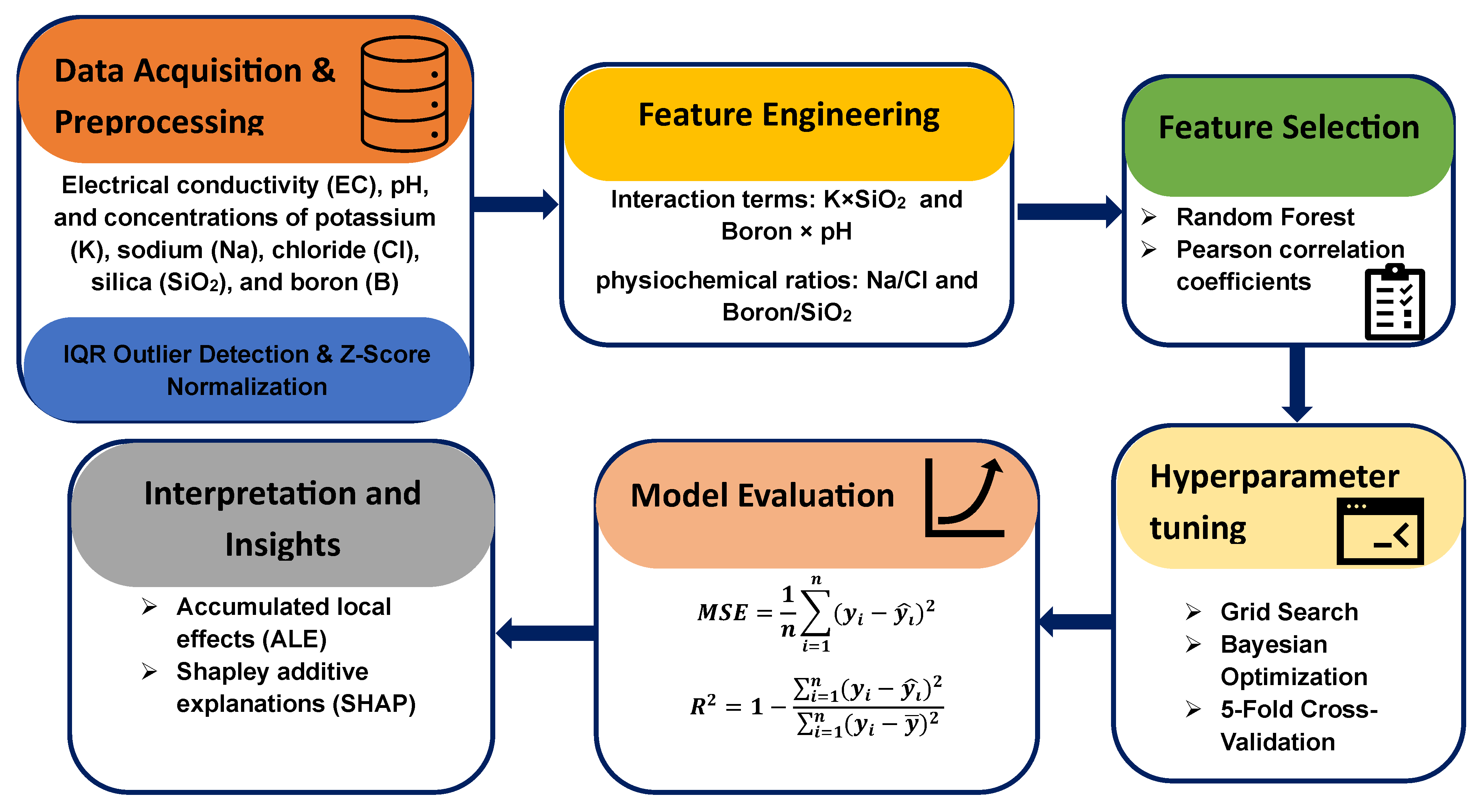
Graph neural networks (GNNs) extend neural networks to graph-structured data, enabling the modeling of relational dependencies [45,46]. In this study, a transformer-based GNN architecture was employed, leveraging self-attention mechanisms to aggregate information from neighboring nodes. The message-passing framework is defined as follows:
h i ( l + 1 ) = σ ( j N ( i ) α i j W ( l ) h i ( l ) )
where hi(l) is the feature vector of node i at layer l, N ( i ) is the set of neighbors of node i, αij is the attention coefficient, and W(l) is the weight matrix. The attention coefficients are computed as [47]:
α i j = e x p ( L e a k y R e L U ( a T [ W h i | | W h j ] ) ) k N ( i ) e x p ( L e a k y R e L U ( a T [ W h i | | W h j ] ) )
where a is a learnable attention vector, and ∥ denotes concatenation. The final node embeddings are used for regression:
y ^ = W o u t h i ( L ) + b o u t .
GNNs are particularly effective for datasets with inherent graph structures, such as molecular data or social networks.

3. Methodology

The dataset utilized in this study comprises 84 geothermal water samples collected from hydrothermal systems within Turkiye, Western Anatolia, encompassing a range of physicochemical conditions and reservoir types. The dataset consisted of hydrogeochemical parameters extracted from refs. [25,48,49,50,51], including electrical conductivity (EC), pH, and concentrations of key ions such as potassium (K), sodium (Na), chloride (Cl), silica (SiO2), and boron (B). The target variable was reservoir temperature. Figure 1 depicts the schematic of the workflow employed in this study. Outliers were identified and treated using interquartile range (IQR) analysis to prevent undue influence on model training. For each feature, the first quartile (Q1, 25th percentile) and third quartile (Q3, 75th percentile) were calculated. The IQR was defined as the difference between these quartiles:
I Q R = Q 3 Q 1 .
Outlier boundaries were then set using the common statistical thresholds:
L o w e r   b o u n d = Q 1 1.5 × I Q R
U p p e r   b o u n d = Q 3 + 1.5 × I Q R .
To ensure a consistent scale across all features, standardization was applied using the Z-score normalization technique:
X = X μ σ
where X represents the raw feature values, μ is the mean, and σ is the standard deviation. This step was particularly important for algorithms sensitive to feature magnitudes, such as SVR and DNN.
Feature engineering was conducted to enhance predictive capability. Interaction terms, including K × SiO2 and Boron × pH, were derived to capture nonlinear relationships. Additionally, physiochemical ratios, such as Na/Cl and Boron/SiO2, were introduced based on domain knowledge of geochemical processes. A small constant (1 × 10⁻¹⁰) was added to denominator terms to prevent division by zero errors. To identify the most informative features, a two-step selection approach was implemented. First, a random forest regressor was trained on the dataset, and feature importance scores were computed using the mean decrease in impurity (Gini importance). Second, absolute Pearson correlation coefficients between each feature and the target variable were calculated. The six most significant features, determined through a combination of these methods, were selected for model training to reduce redundancy and mitigate multicollinearity.
All models were trained on 80% of the dataset, while the remaining 20% was used for testing. Stratified sampling was applied to maintain the distribution of reservoir temperatures across the training and test sets. To ensure optimal model performance, hyperparameter tuning was conducted using a combination of grid search and Bayesian optimization.
The DNN was designed with multiple fully connected layers, ranging from three to five, each containing between 64 and 256 neurons. The input layer incorporated both original hydrogeochemical variables and their interaction terms explicitly, facilitating the model’s capacity to learn nonlinear dependencies. Rectified linear unit (ReLU) activation functions were employed to introduce nonlinearity within the network. The Adam optimizer was selected due to its efficiency and adaptive learning capabilities, with learning rates systematically explored in the range of 1 × 10⁻⁴ to 1 × 10⁻³. To prevent overfitting and improve generalization, dropout regularization was applied with rates varying between 0.2 and 0.5, and L2 weight decay was incorporated with regularization coefficients from 1 × 10⁻⁵ to 1 × 10⁻³. Additionally, batch normalization was implemented after each hidden layer to promote stable and accelerated training convergence. Training was performed with mini-batches of size 32, and early stopping based on validation loss was used to avoid overfitting.
The GNN approach sought to model the relational structure among hydrogeochemical features and their interactions by representing each feature and interaction as nodes within a graph. Edges were established based on expert knowledge regarding chemical affinities and statistical correlations, aiming to encode meaningful connections within the data. The GNN architecture comprised two to four graph convolutional layers, with hidden feature dimensions ranging from 32 to 128. Variants of graph convolutions, including graph convolutional networks (GCNs) and graph attention networks (GATs), were investigated to weigh neighbor contributions dynamically. Similar to the DNN, the Adam optimizer was utilized with learning rates between 1 × 10⁻⁴ and 1 × 10⁻³. Dropout and L2 weight decay regularization techniques were also applied to mitigate overfitting. Training employed early stopping criteria with mini-batch adjustments to optimize learning dynamics.
The models were evaluated through five-fold cross-validation, wherein the dataset was split into five subsets, each serving as a validation set once while the others were used for training. The evaluation metric was mean squared error (MSE):
M S E = 1 n i = 1 n ( y i y i ^ ) 2
where yi represents the actual temperature and y i ^ is the predicted value. The coefficient of determination (R2) was also computed to assess model explanatory power:
R 2 = 1 i = 1 n ( y i y i ^ ) 2 i = 1 n ( y i y ¯ ) 2
where y ¯ is the mean observed temperature. Models were selected based on their generalization performance, ensuring that they did not overfit the training data while maintaining high predictive accuracy.

4. Results and Discussion

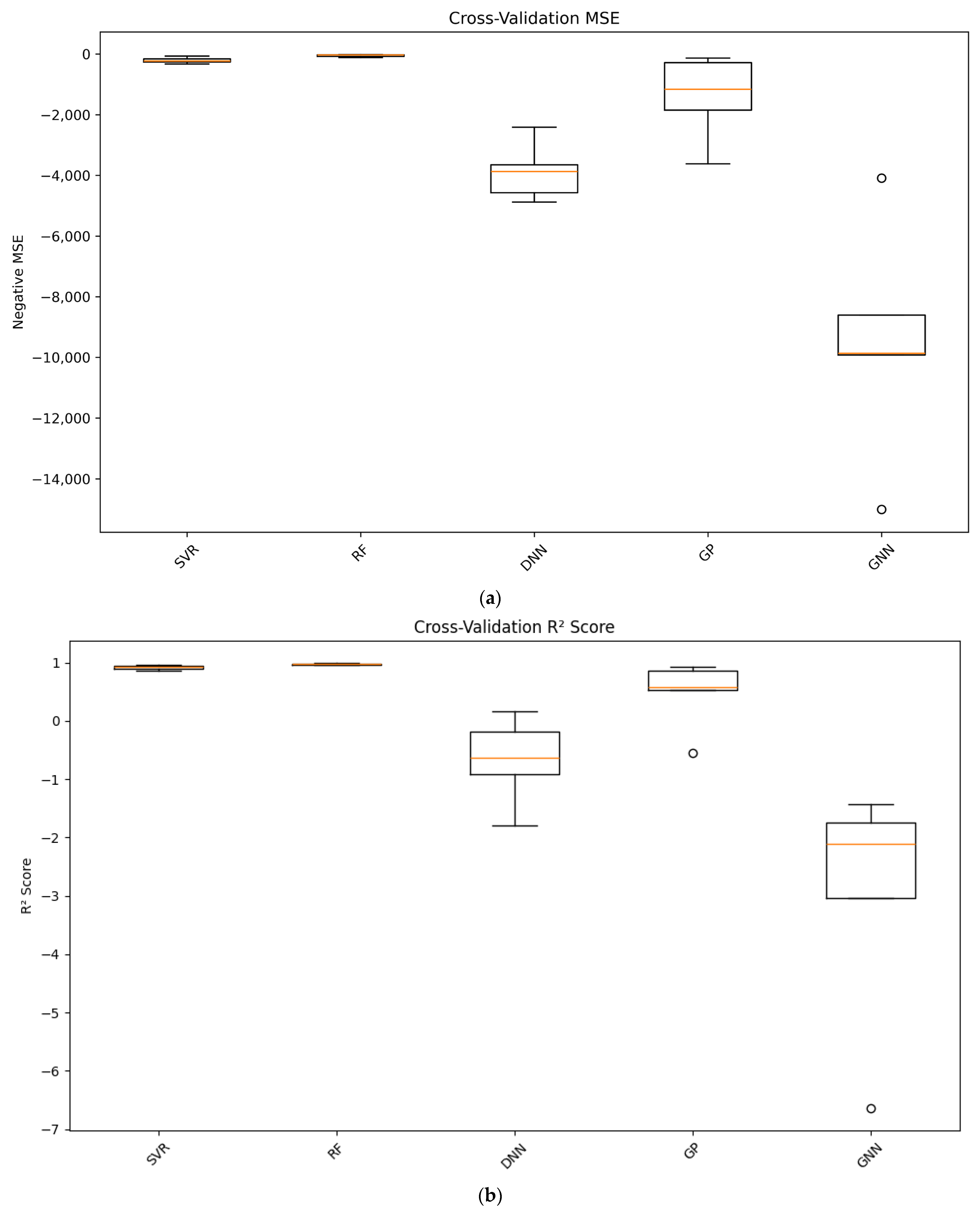
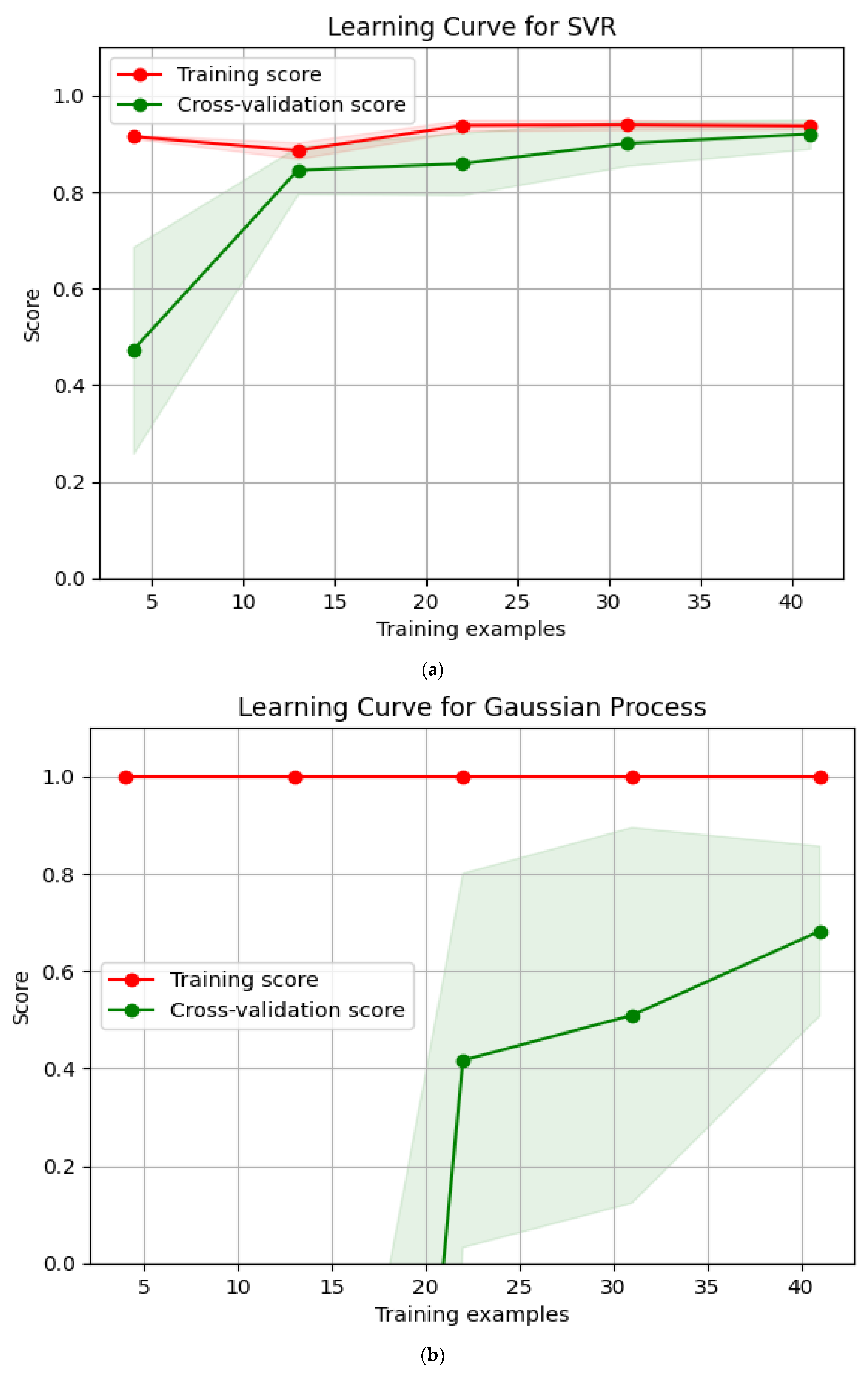
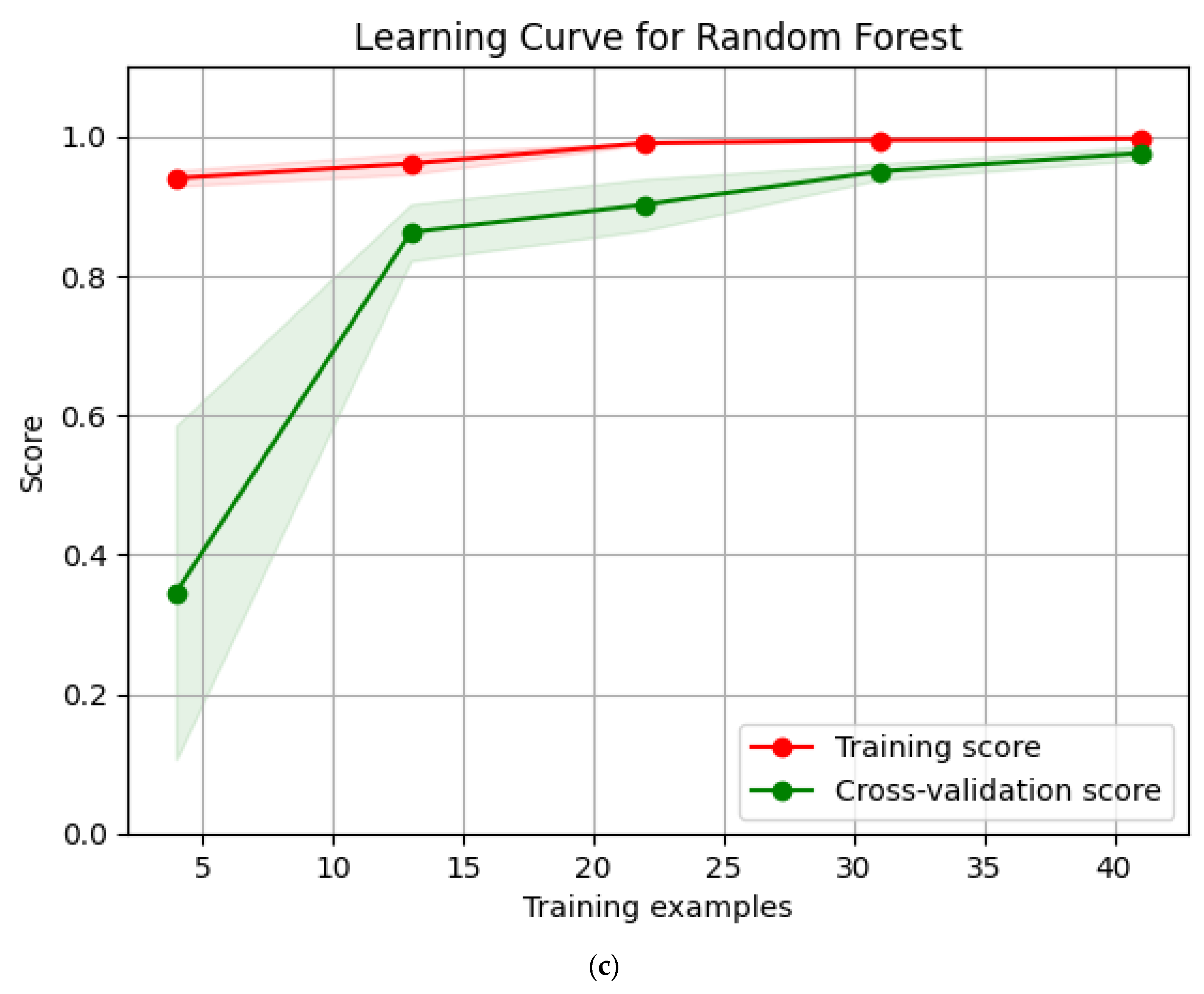
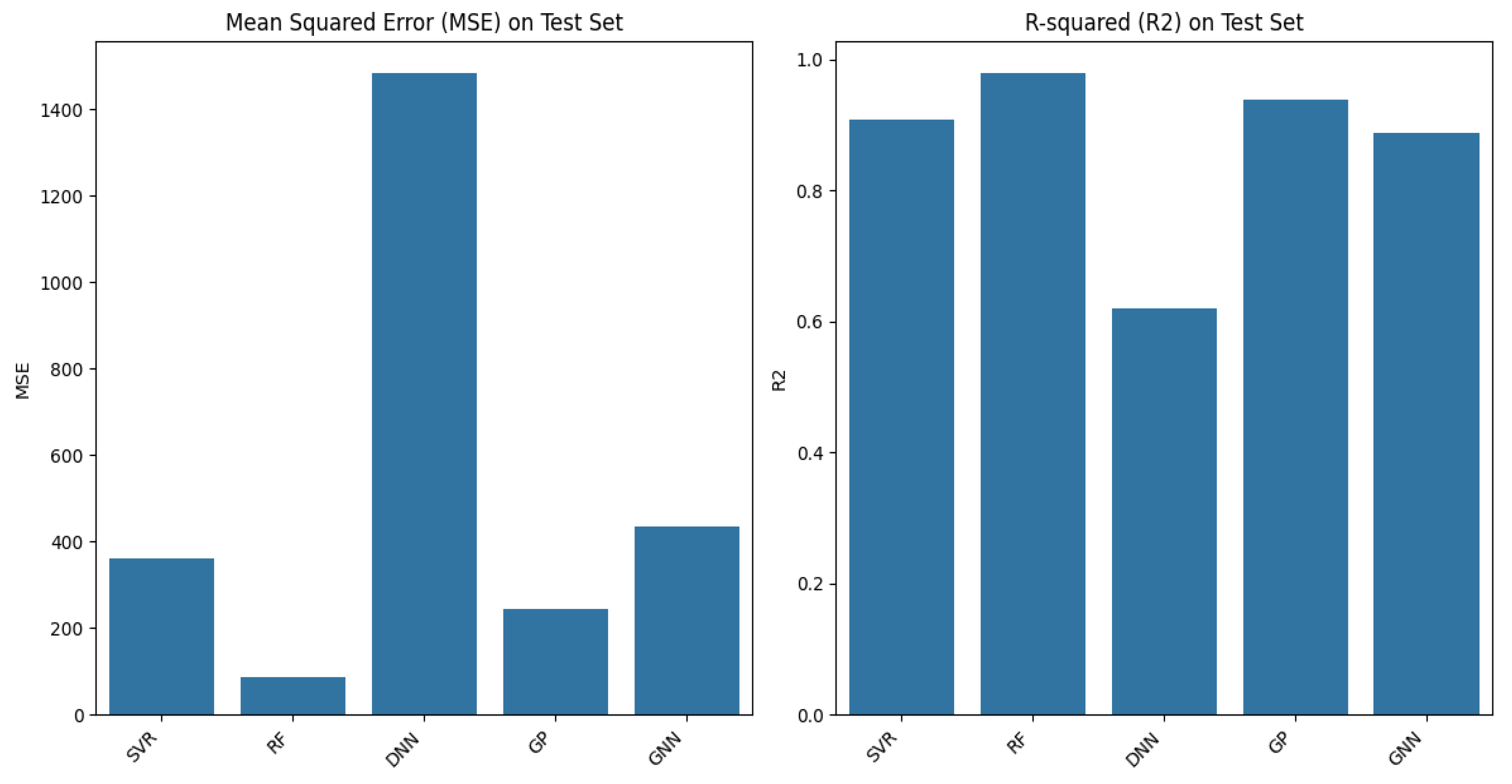
4.1. Comparison of Model Prediction Performance

Figure 2 presents the cross-validation results for multiple machine learning models, comparing their performance in terms of MSE and R2 score. In Figure 2a, the MSE values obtained from cross-validation for each machine learning model are illustrated. The RF model emerges as the clear frontrunner, exhibiting the lowest MSE, which substantiates its efficacy in minimizing prediction errors. This performance is attributed to the RF’s ensemble learning approach, which adeptly captures intricate nonlinear relationships that are characteristic of geothermal data. Contrastingly, the performance of the DNN and GNN models is marked by higher MSE values and greater variability. This suggests that these models may be prone to overfitting, undermining their reliability in terms of generalizability across diverse datasets. Furthermore, while the GP model showcases moderate performance with an MSE that is significantly higher than RF, it illustrates the potential for better handling data variability, although with limitations. Figure 2b presents boxplot representations of the R2 scores, further explaining the predictive performance of the evaluated models. The RF consistently achieves R2 scores approaching 1, reflecting its robust ability to explain the variance in reservoir temperature effectively. This aligns with the foundational principles of RF in harnessing multiple decision trees to synthesize insights from different facets of the data. The SVR model, while demonstrating commendable R2 scores, shows a slightly wider spread among its scores, suggesting its adaptability in varying scenarios, but with inherent uncertainties. In stark contrast, the DNN and GNN exhibit significantly lower and more inconsistent R2 scores, which indicates their susceptibility to issues related to bias and variance, primarily driven by the challenges of hyperparameter optimization and the sizes of the training datasets employed. The comparative performance trends illustrated in Figure 3, which compares both MSE and R2 across the models, highlight the critical trade-offs between bias and variance experienced by each predictive framework. The pronounced shifts depicted in the MSE and R2 for DNN and GNN exemplify the struggles these models face in achieving a balance between closely fitting the training data and maintaining generalizability. In contrast, the RF model is characterized by a relatively stable trajectory between MSE and R2, reinforcing its strength in striking a favorable bias-variance balance.
Figure 4 illustrates the learning curves for three machine learning models, SVR, GP, and RF, highlighting their training and cross-validation performance. As shown in Figure 4a, the SVR model maintains a consistently high training score, suggesting that it fits the training data well. However, its cross-validation score exhibits a steady upward trend, indicating that as more data become available, the model improves its ability to generalize. The relatively small gap between training and validation scores suggests that SVR is relatively stable, though the slight divergence may indicate mild overfitting, particularly when dealing with limited data. As depicted in Figure 4b, the GP model, on the other hand, initially exhibits significant performance instability, as seen in the wide variance of its cross-validation scores. With a small number of training examples, the model struggles to generalize, resulting in poor cross-validation performance. However, as additional training data are incorporated, the cross-validation score improves, and variance reduces, indicating that the model benefits substantially from larger datasets. The persistently high training score suggests that the GP model has high model complexity, which, when coupled with small datasets, leads to overfitting. The progressive convergence of training and validation scores with increasing data suggests that GP models require a substantial amount of training examples to enhance their predictive reliability. As demonstrated in Figure 4c, the RF model exhibits strong generalization characteristics compared to the other two models. While its training score remains consistently high, its cross-validation score also increases with additional training data, leading to a reduced gap between training and validation scores. This suggests that the RF model effectively learns from new data while maintaining robust generalization capabilities. The relatively narrow shaded region in the RF learning curve implies lower variance, suggesting that the model is less sensitive to fluctuations in training data compared to GP.
The evaluation of model performance, as illustrated in Figure 5, provides critical insights into the predictive accuracy and reliability of the machine learning algorithms employed in this study. The mean squared error (MSE) and R-squared (R2) metrics on the test dataset serve as robust indicators of model efficacy, with lower MSE values and higher R2 scores reflecting superior predictive capability. Among the models evaluated—support vector regression (SVR), random forest (RF), deep neural networks (DNN), Gaussian process regression (GP), and graph neural networks (GNN)—the results reveal a clear hierarchy in performance. RF emerged as the most accurate algorithm, achieving the lowest MSE (66.16) and the highest R2 score (0.977), highlighting its ability to effectively capture the complex, nonlinear relationships within the dataset. This superior performance can be attributed to RF’s ensemble learning approach, which leverages multiple decision trees to handle feature interactions and nonlinearities inherent in geothermal data. SVR, optimized with a linear kernel, demonstrated respectable accuracy (MSE 209.67, R2 0.919), reflecting its robustness for this dataset. In contrast, DNN struggled, with negative R2 values suggesting potential overfitting or an inadequate model structure for the data. Similarly, the GNN approach, though innovative, failed to deliver the expected predictive results, possibly due to the simplistic graph construction methodology employed. GP provided moderate performance, offering probabilistic insights into prediction uncertainties, but falling short of RF’s accuracy.
Figure 6 presents scatter plots comparing actual and predicted reservoir temperatures for each model accompanied by 95% confidence intervals. A strong alignment of data points along the 1:1 line indicates high predictive accuracy, while wider confidence bands signify greater uncertainty. As depicted in Figure 6a, SVR demonstrates a reasonable alignment between predicted and actual values with a moderate confidence interval width. The model exhibits acceptable predictive capability, but shows some deviation at extreme values, indicating possible limitations in capturing nonlinear dependencies within the dataset. As shown in Figure 6b, RF achieves improved performance over SVR, with predictions closely following the 1:1 line and narrower confidence intervals. The model effectively captures complex relationships in the data but may still be susceptible to slight overfitting. As demonstrated in Figure 6c, DNN shows a wider confidence interval than RF, suggesting variability in its predictions. This could be attributed to the model’s sensitivity to hyperparameter tuning and the need for extensive training data to generalize effectively. GP provides robust predictive performance, with narrower confidence intervals than DNN and reasonable alignment with actual values, as shown in Figure 6d. The probabilistic nature of GP contributes to well-calibrated uncertainty estimations. GNN exhibits comparable accuracy to GP, though the confidence interval width suggests slight inconsistencies in predictions (See Figure 6e).

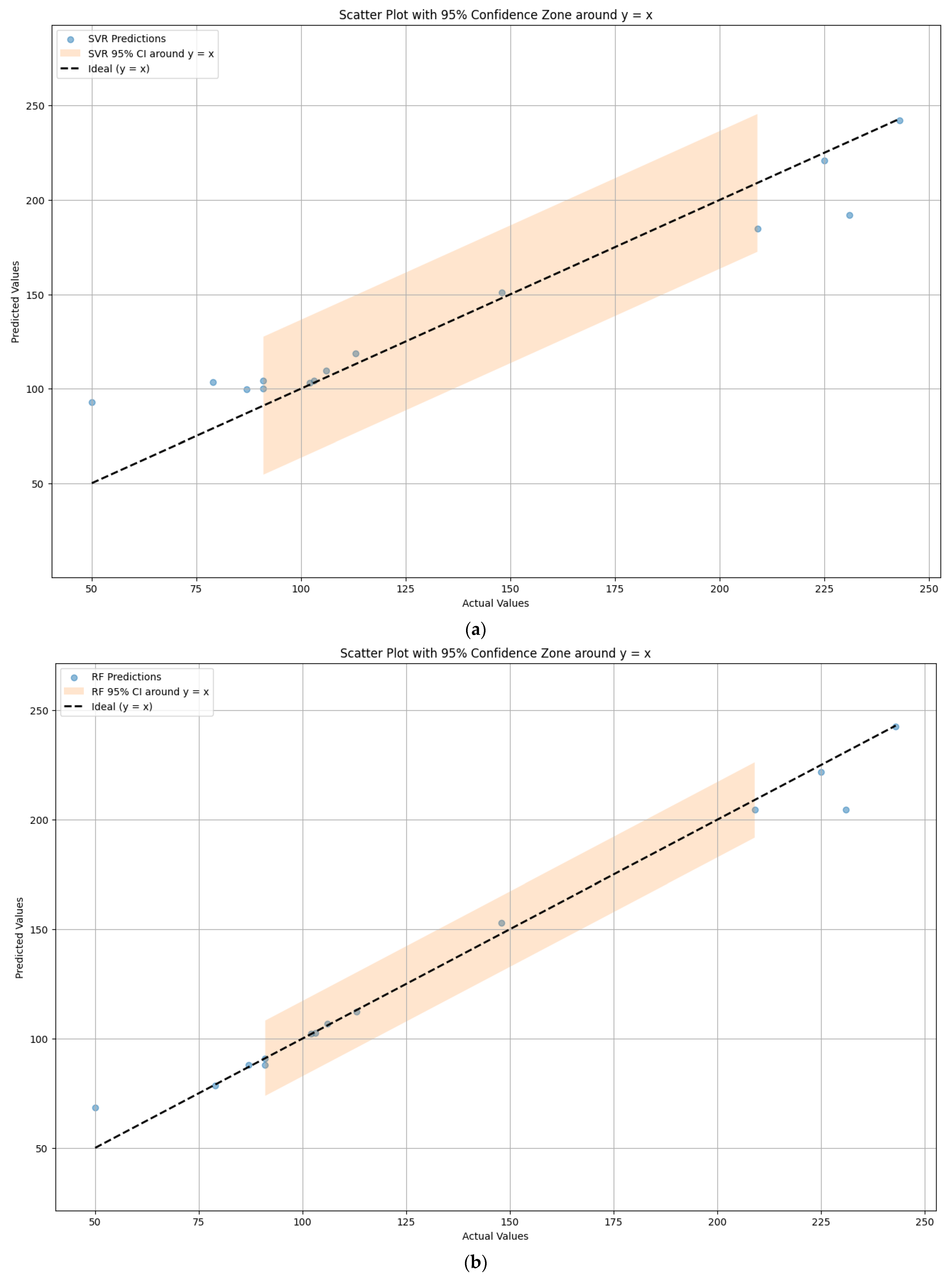
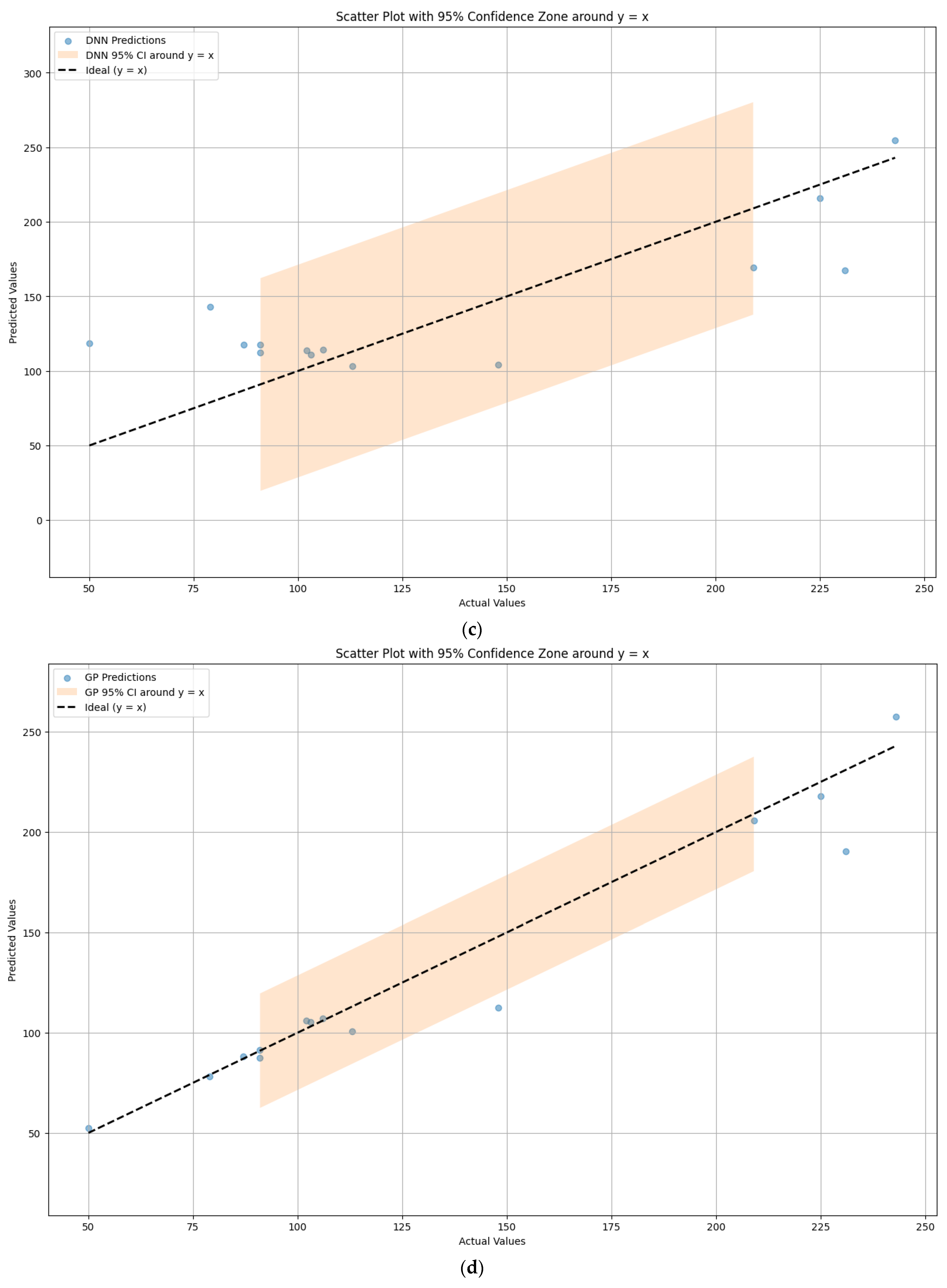
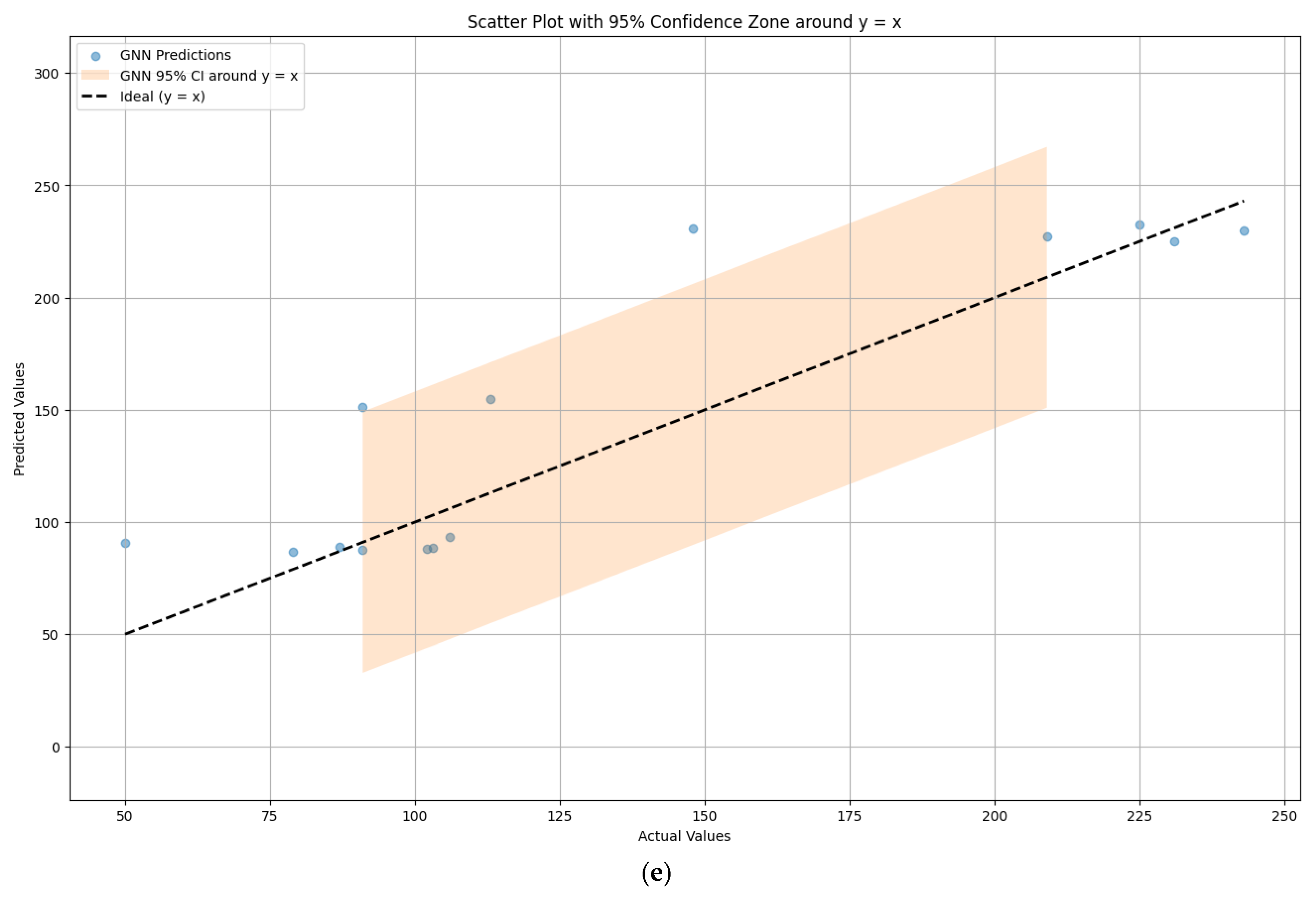
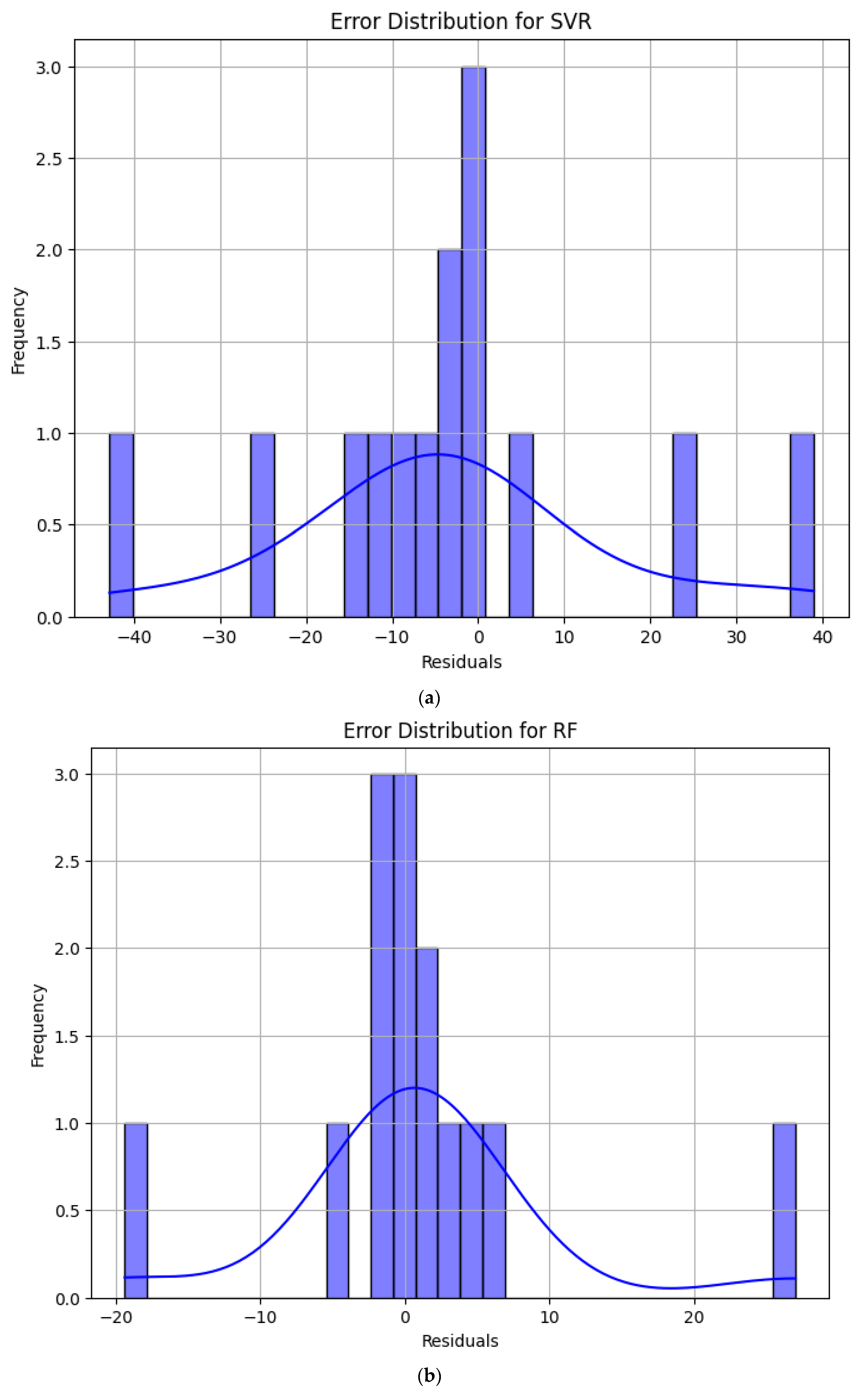
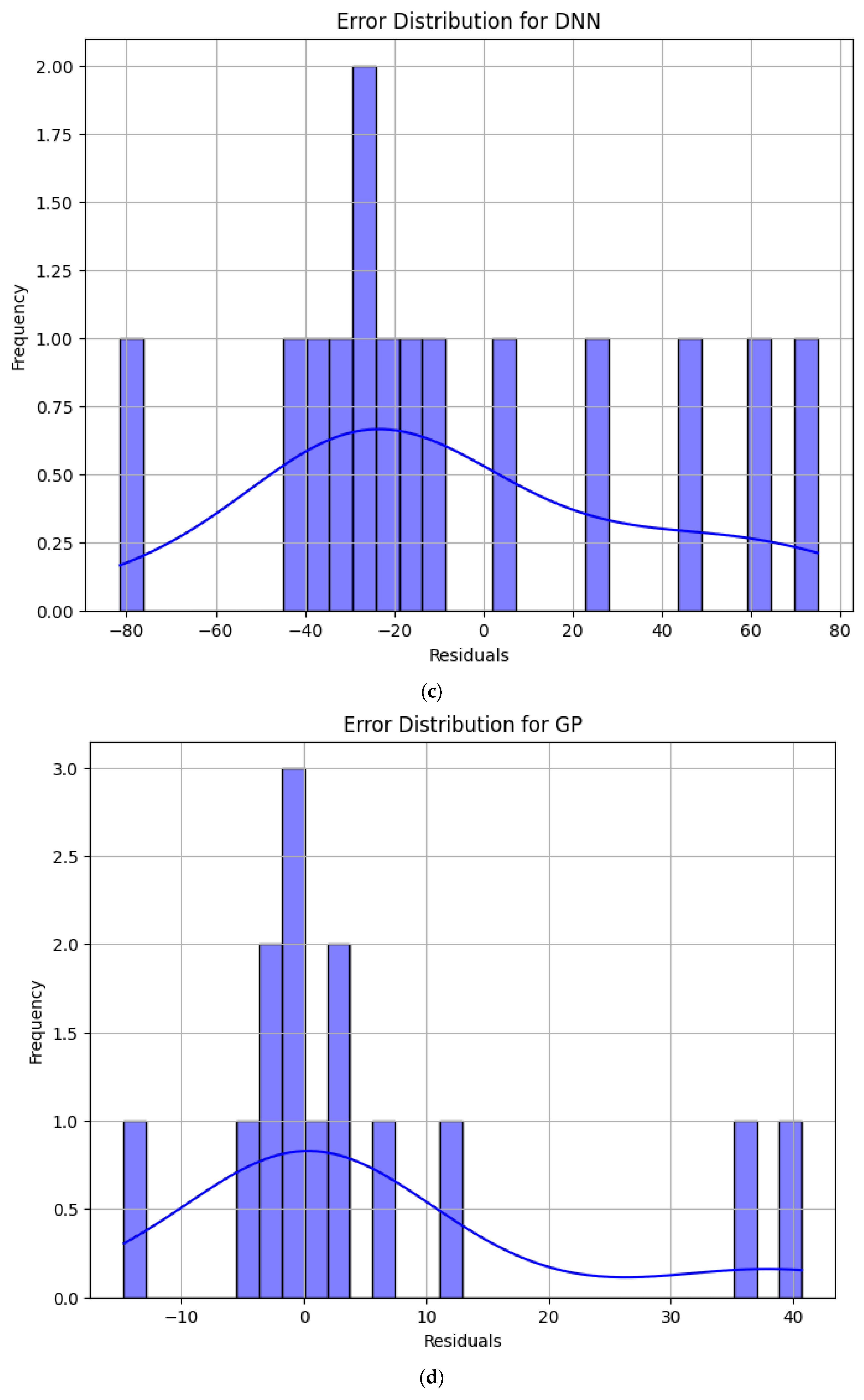
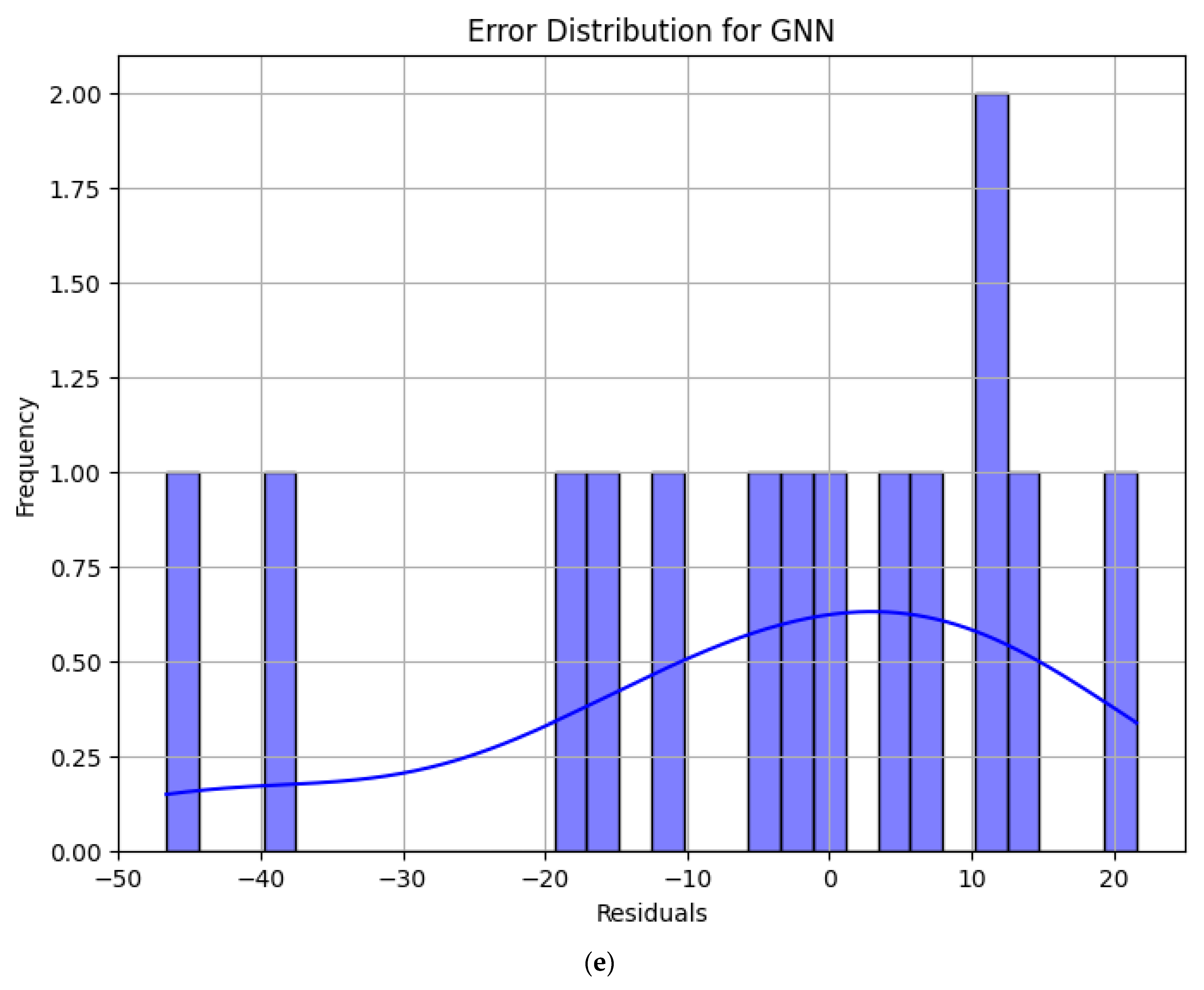
4.2. Error Analysis of Model Prediction Results

Figure 7 presents the error distributions (residuals) for each model, providing deeper insights into their predictive reliability and potential biases. As shown in Figure 7a, SVR displays a relatively dispersed error distribution, with a tendency toward overestimation and underestimation at extreme values. The non-Gaussian shape suggests model biases that could affect predictive reliability. As depicted in Figure 7b, RF exhibits a more symmetric error distribution centered around zero, indicating minimal systematic bias and better overall prediction stability compared to SVR. As demonstrated in Figure 7c, DNN presents a more dispersed residual distribution with noticeable skewness, reflecting instances where the model fails to generalize well. GP achieves a relatively balanced error distribution with a clear peak around zero, reinforcing its ability to capture underlying data trends effectively (See Figure 7d). GNN shows a wider and less structured residual distribution, as illustrated in Figure 7e, which may suggest sensitivity to complex spatial relationships within geothermal reservoirs.
Further validation is achieved using more extensive and geographically diverse datasets.
The wide confidence intervals observed in Figure 6, particularly for the DNN and GNN models, can be attributed to the variability and dispersion in their error distributions as shown in Figure 7. These broader confidence bands indicate a higher degree of predictive uncertainty, which aligns with the residual patterns evident in the corresponding models. For instance, the DNN’s error distribution (Figure 7c) reveals a noticeable skew and wider spread, suggesting inconsistencies in its generalization capability and increased sensitivity to specific input features or hyperparameter configurations. Similarly, GNN’s residuals (Figure 7e) demonstrate greater dispersion and lack of symmetry, which may stem from its architectural limitations in fully capturing the spatial dependencies within the geothermal dataset. These characteristics contribute directly to the wider predictive intervals observed in Figure 6, reflecting the models’ uncertainty in estimating reservoir temperature. In contrast, models such as RF and GP, which exhibit narrower and more symmetric error distributions centered around zero (Figure 7b,d), yield tighter confidence intervals in Figure 6. This reinforces the relationship between error distribution shape and predictive certainty, underscoring the importance of residual analysis in diagnosing uncertainty sources in model outputs.

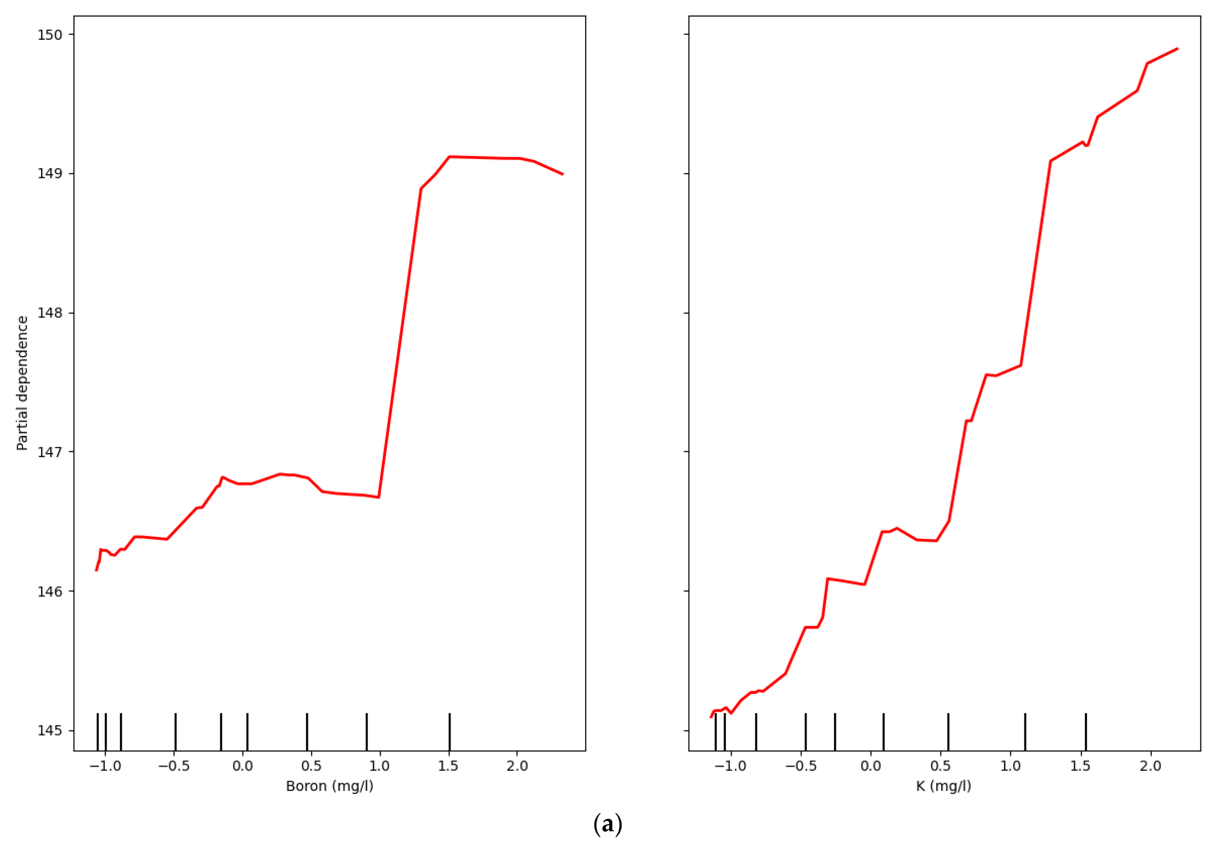
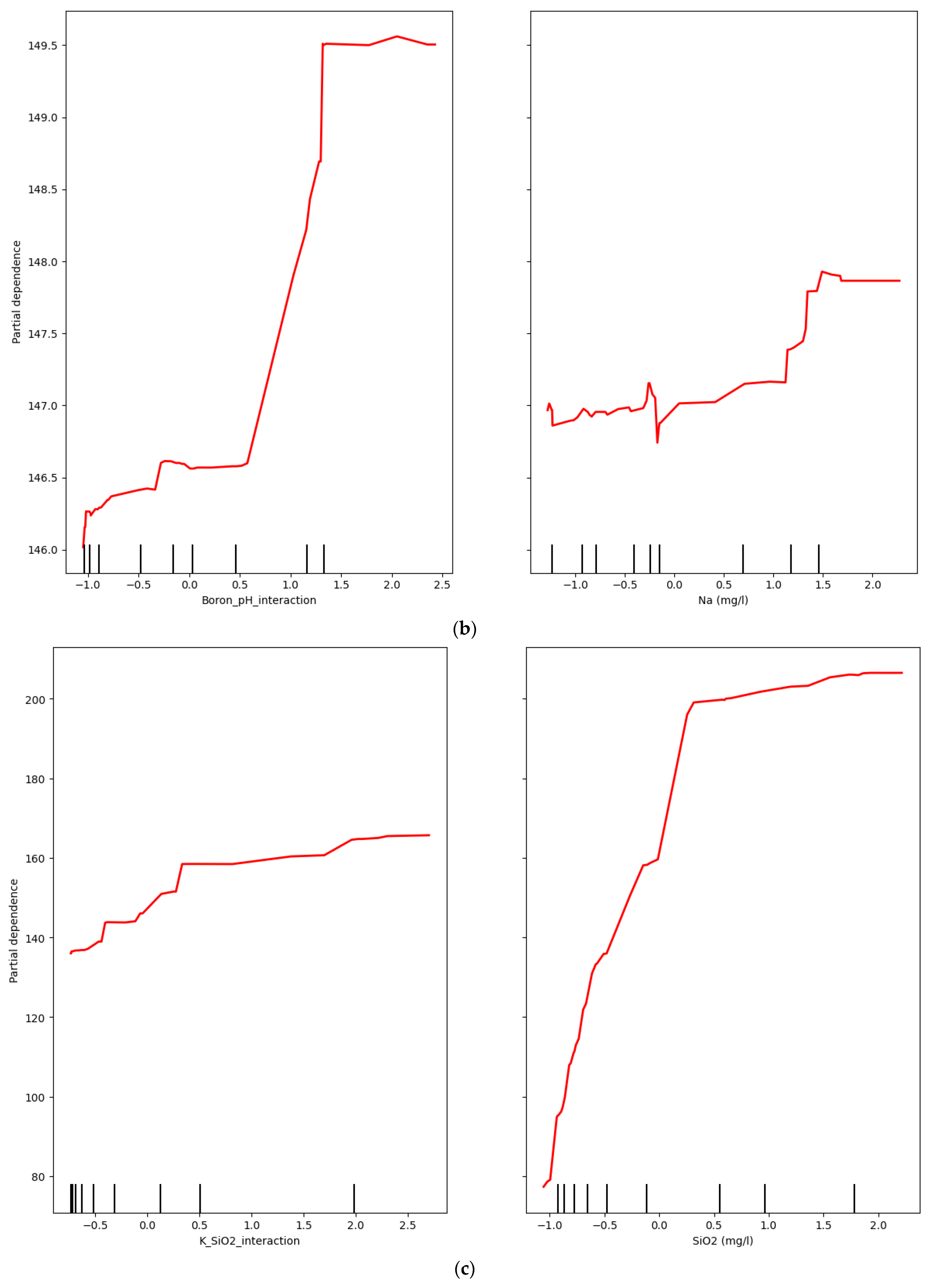
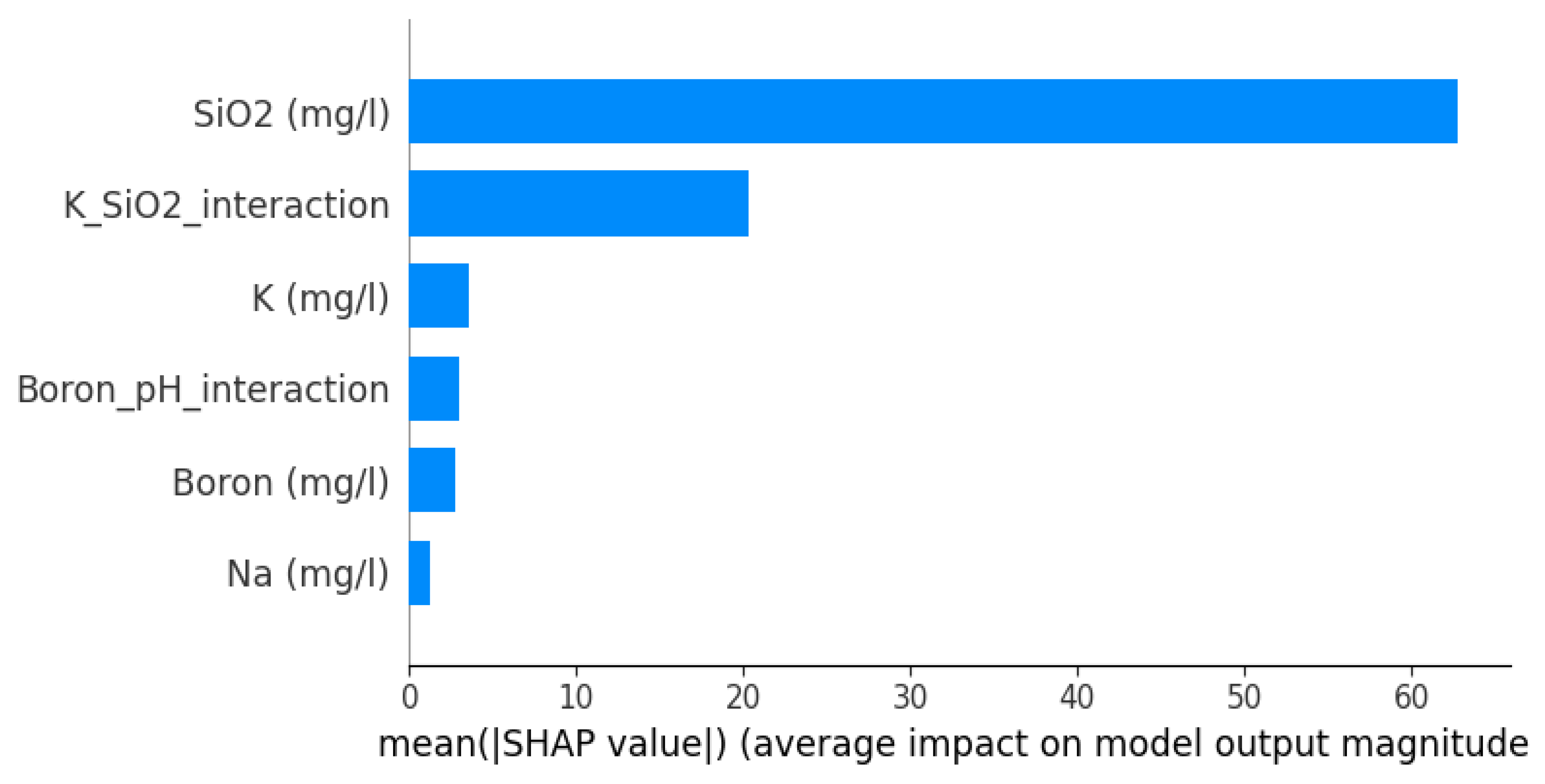
4.3. Analysis of Model Interpretability

Figure 8 presents the partial dependence plots (PDPs) illustrating the impact of individual hydrogeochemical features on the predicted reservoir temperature. These plots provide critical insights into the nonlinear relationships between key input variables and temperature predictions, enhancing model interpretability and validating domain knowledge in geothermal systems. In Figure 8a, the contributions of boron (B) and potassium (K) are analyzed. The observed trends indicate that higher concentrations of these elements positively influence predicted temperature, suggesting their strong correlation with geothermal processes. Boron exhibits a gradual increase in temperature response, followed by a sharp rise at higher concentrations, suggesting a potential threshold effect. Potassium demonstrates a more consistent upward trend, highlighting its relevance in geothermal fluid interactions and mineral equilibria. Figure 8b examines the effects of boron-pH interaction and sodium (Na) concentration. The boron-pH interaction displays a distinct threshold effect, where a sharp increase in temperature is observed beyond a specific concentration range, emphasizing the complex interplay between chemical equilibria and geothermal fluid dynamics. The Na concentration exhibits a moderate yet nonlinear influence on temperature, reflecting its role in deep hydrothermal circulation and mineral dissolution processes. Figure 8c focuses on the interaction between potassium and silica (K-SiO2), as well as the standalone effect of SiO2 concentration. The K-SiO2 interaction reveals a strong nonlinear influence, suggesting that their combined presence in geothermal fluids significantly impacts temperature prediction. SiO2 concentration exhibits a steep and nearly exponential increase in predicted temperature, reinforcing its role as a key geochemical indicator. This trend underscores the importance of silica solubility equilibria in geothermal reservoirs, where higher temperatures promote increased silica dissolution and transport. The sharp rise in temperature response at low SiO2 concentrations suggests a critical threshold effect, beyond which geothermal fluid equilibria shift significantly.
To enhance interpretability, SHAP values were employed to quantify the contribution of each feature to model predictions. Additionally, the SHAP values provide a more granular understanding of how individual features impact predictions, with certain features consistently exerting a positive or negative influence. This method enabled a deeper understanding of how hydrogeochemical variables influenced reservoir temperature estimation. The SHAP values were computed using the Python 3.9.21 SHAP library, which implements the tree explainer method optimized for ensemble tree-based models such as random forest. Default parameter settings were employed, except for setting “feature perturbation” to “tree path dependent”, to improve explanation accuracy specific to tree ensembles. The analysis involved generating SHAP values for the entire test dataset to capture the global impact of features, followed by the creation of summary plots to rank feature importance based on mean absolute SHAP values. This approach ensured reproducibility and facilitated comprehensive insight into feature interactions and their nonlinear effects on reservoir temperature predictions. Figure 9 presents the SHAP summary plot, ranking features by their mean absolute SHAP value, which quantifies their contribution to model predictions. SiO2 concentration emerges as the most influential predictor, followed by interaction effects between potassium and silica. The ranking aligns with domain knowledge, reinforcing the model’s ability to capture underlying geochemical processes.
While the RF model exhibited outstanding predictive accuracy in this study, evidenced by the lowest MSE and highest R2 scores across cross-validation and test datasets, it is essential to critically examine its inherent limitations and deployment challenges. A primary concern relates to computational efficiency and scalability. The RF algorithm constructs and aggregates numerous decision trees to form an ensemble, a process that, while effective in modeling nonlinear patterns typical of geothermal systems, suffers significant computational and memory demands as data dimensionality increases. This issue is especially relevant when dealing with large-scale or high-resolution hydrogeochemical datasets, where the computational burden may impede timely training and model updates. Furthermore, RF does not conduct embedded feature selection, often utilizing all input variables regardless of their predictive relevance. This can lead to inefficiencies in model computation and hinder interpretability, particularly in cases involving redundant or weakly informative features. In practical deployment scenarios, RF generally achieves faster inference than deep learning methods; however, the need to traverse multiple decision trees for each prediction can still cause latency, which may be problematic in real-time or resource-constrained environments such as field-deployed monitoring systems. Therefore, while the RF model offers a compelling balance of accuracy and generalizability, its computational demands and real-time deployment limitations must be carefully managed to ensure effective integration into operational geothermal exploration and monitoring frameworks.
While the dataset captures meaningful variability within the target geothermal region, its relatively limited sample size imposes certain constraints on the generalizability of the developed models. Specifically, the ability to extend the predictive framework to other geothermal provinces with different geological or tectonic settings may be limited without additional regional calibration. Therefore, the models demonstrate strong performance within the scope of the available data.

5. Conclusions

The present study undertook a thorough evaluation of various advanced machine learning models to predict reservoir temperature in geothermal systems based on hydrogeochemical parameters. The comparison focused on five models: random forest (RF), support vector regression (SVR), deep neural networks (DNN), Gaussian process regression (GP), and graph neural networks (GNN). Through rigorous cross-validation and performance assessment, several critical findings emerged, emphasizing the importance of model selection and feature engineering in the context of geothermal data.
The RF model distinguished itself as the most effective predictive algorithm, achieving the lowest MSE and the highest R2 score among the evaluated models. Its ensemble learning strategy enables the RF model to adeptly capture the complex, nonlinear relationships inherent in geothermal datasets. In contrast, the DNN and GNN models displayed higher MSE values and inconsistencies, suggesting challenges in generalizability and potential overfitting—a common concern with deep learning architectures reliant on hyperparameter tuning and extensive datasets.
The learning curves for SVR, GP, and RF further illuminated the predictive capacities of these models. The consistency and stability in RF’s performance highlight its capacity to generalize well with increasing data, unlike the GP model, which exhibited substantial improvements with larger datasets but struggled initially due to high model complexity. SVR, while indicative of moderate overfitting, maintained a steady trajectory in cross-validation scores, suggesting its adaptability.
Analysis of predictive accuracy through metrics such as MSE and R2 revealed a distinct hierarchy in performance. While SVR exhibited respectable results, the DNN and GNN models consistently failed to achieve satisfactory predictive accuracy. The evaluation reaffirms the necessity of choosing machine learning models not only based on their theoretical applicability, but also on performance outcomes in specific datasets. Another noteworthy aspect of this study was the exploration of error distributions across models. The RF model demonstrated a well-balanced error distribution, minimizing systematic bias, while the DNN and GNN models faced challenges regarding predictive variability and bias.
Additionally, the investigation into hydrogeochemical features through partial dependence plots (PDPs) and SHAP value analysis unveiled critical relationships influencing reservoir temperature predictions. Notably, silica concentration emerged as a key predictor, followed by interaction terms such as K × SiO2, underscoring the importance of geochemical factors in geothermal systems. The results align with established domain knowledge, suggesting that effective feature engineering can enhance both the predictive accuracy and interpretability of machine learning models in this field.
The findings of this research underscore the transformative potential of machine learning in geothermal reservoir characterization. The identification of key geochemical features and their influence on temperature estimation not only enhances predictive accuracy, but also contributes to a deeper understanding of hydrothermal system dynamics. This knowledge can be instrumental in optimizing geothermal exploration, facilitating the identification of promising geothermal sites, and improving reservoir management strategies.

Funding

This research received no external funding.

Data Availability Statement

Data will be made available on request to the author.

Conflicts of Interest

The author declares no conflict of interest.

Nomenclature

Abbreviations
ALE Accumulated local effects
ANNs Artificial neural networks
BHT Bottom-hole temperature
BPNN Back propagation neural network
DNN Deep neural networks
ELM Extreme learning machine
GMDH Group method of data handling
GNN Graph neural networks
GCNs Graph convolutional networks
GATs Graph attention networks
GP Gaussian process regression
GRNNGeneralized regression neural network
IQR Interquartile range
MAE Mean absolute error
ML Machine learning
NGB Natural gradient boosting
RF Random forest
RMSE Root mean square error
SFT Static formation temperatures
SHAP Shapley additive explanations
SVR Support vector regression
Variables
T b ( x ) Prediction of the b-th tree
y ^ Average of the predictions
σ n 2 Noise variance
aLearnable attention vector
a(l−1)Activation from the previous layer
bBias term
Bnumber of trees
b(l)Bias vector for layer l
g(l)Activation function
hi(l)Feature vector of node i at layer l
K (X, X) Kernel matrix
k(x,x′) Covariance function
m(x) Mean function
wWeight vector
W(l)Weight matrix
W(l)Weight matrix for layer l
XRaw feature value
αijAttention coefficient
γKernel coefficient
ΔImpurity (f, t)Reduction in variance due to splitting on feature f at node t
μMean of feature
ξi, ξiSlack variables
σStandard deviation of feature
ϕ(xi) Mapping to a higher-dimensional feature space
N ( i ) Set of neighbors of node i

References

  1. Younger, P.L. Geothermal Energy: Delivering on the Global Potential. Energies 2015, 8, 11737–11754. [Google Scholar]
  2. Anderson, A.; Rezaie, B. Geothermal technology: Trends and potential role in a sustainable future. Appl. Energy 2019, 248, 18–34. [Google Scholar] [CrossRef]
  3. Liu, Z.; Wu, M.; Zhou, H.; Chen, L.; Wang, X. Performance evaluation of enhanced geothermal systems with intermittent thermal extraction for sustainable energy production. J. Clean. Prod. 2024, 434, 139954. [Google Scholar] [CrossRef]
  4. Izadi, G.; Freitag, H.-C. Resource assessment and management for different geothermal systems (hydrothermal, enhanced geothermal, and advanced geothermal systems). In Geothermal Energy Engineering; Elsevier: Amsterdam, The Netherlands, 2025; pp. 23–72. [Google Scholar]
  5. Wang, K.; Yuan, B.; Ji, G.; Wu, X. A comprehensive review of geothermal energy extraction and utilization in oilfields. J. Pet. Sci. Eng. 2018, 168, 465–477. [Google Scholar] [CrossRef]
  6. Song, G.; Shi, Y.; Xu, F.; Song, X.; Li, G.; Wang, G.; Lv, Z. The magnitudes of multi-physics effects on geothermal reservoir characteristics during the production of enhanced geothermal system. J. Clean. Prod. 2024, 434, 140070. [Google Scholar] [CrossRef]
  7. Sharmin, T.; Khan, N.R.; Akram, M.S.; Ehsan, M.M. A state-of-the-art review on geothermal energy extraction, utilization, and improvement strategies: Conventional, hybridized, and enhanced geothermal systems. Int. J. Thermofluids 2023, 18, 100323. [Google Scholar] [CrossRef]
  8. Muñoz, G.; Bauer, K.; Moeck, I.; Schulze, A.; Ritter, O. Exploring the Groß Schönebeck (Germany) geothermal site using a statistical joint interpretation of magnetotelluric and seismic tomography models. Geothermics 2010, 39, 35–45. [Google Scholar] [CrossRef]
  9. Spichak, V.; Manzella, A. Electromagnetic sounding of geothermal zones. J. Appl. Geophys. 2009, 68, 459–478. [Google Scholar] [CrossRef]
  10. Bundschuh, J.; Arriaga, M.S. Introduction to the Numerical Modeling of Groundwater and Geothermal Systems; CRC Press: London, UK, 2010; Volume 10, p. b10499. [Google Scholar]
  11. Anderson, M.P.; Woessner, W.W.; Hunt, R.J. Applied Groundwater Modeling: Simulation of Flow and Advective Transport; Academic Press: Cambridge, MA, USA, 2015. [Google Scholar]
  12. Ranjbarzadeh, R.; Sappa, G. Numerical and Experimental Study of Fluid Flow and Heat Transfer in Porous Media: A Review Article. Energies 2025, 18, 976. [Google Scholar] [CrossRef]
  13. Huntington, K.W.; Lechler, A.R. Carbonate clumped isotope thermometry in continental tectonics. Tectonophysics 2015, 647, 1–20. [Google Scholar] [CrossRef]
  14. Guan, B.; Xia, J.; Liu, Y.; Zhang, H.; Zhou, C. Near-surface radial anisotropy tomography of geothermal reservoir using dense seismic nodal array. J. Phys. Conf. Ser. 2023, 2651, 012023. [Google Scholar] [CrossRef]
  15. Jia, X.; Lin, Y.; Ouyang, M.; Wang, X.; He, H. Numerical simulation of hydrothermal flow in the North China Plain: A case study of Henan Province. Geothermics 2024, 118, 102910. [Google Scholar] [CrossRef]
  16. Kadri, M.; Muztaza, N.M.; Nordin, M.N.M.; Zakaria, M.T.; Rosli, F.N.; Mohammed, M.A.; Zulaika, S. Integrated geophysical methods used to explore geothermal potential areas in Siogung-Ogung, North Sumatra, Indonesia. Bull. Geol. Soc. Malays. 2023, 76, 47–53. [Google Scholar] [CrossRef]
  17. Buster, G.; Siratovich, P.; Taverna, N.; Rossol, M.; Weers, J.; Blair, A.; Huggins, J.; Siega, C.; Mannington, W.; Urgel, A. A new modeling framework for geothermal operational optimization with machine learning (Gooml). Energies 2021, 14, 6852. [Google Scholar] [CrossRef]
  18. Khaled, M.S.; Wang, N.; Ashok, P.; van Oort, E.; Wisian, K. Real-time prediction of bottom-hole circulating temperature in geothermal wells using machine learning models. Geoenergy Sci. Eng. 2024, 238, 212891. [Google Scholar] [CrossRef]
  19. Otchere, D.A.; Latiff, A.H.A.; Taki, M.Y.; Dafyak, L.A. Machine-learning-based proxy modelling for geothermal field development optimisation. In Proceedings of the Offshore Technology Conference, Houston, TX, USA, 1–4 May 2023; p. D021S027R004. [Google Scholar]
  20. Ahmadi, M. Advancing Geotechnical Evaluation of Wellbores: A Robust and Precise Model for Predicting Uniaxial Compressive Strength (UCS) of Rocks in Oil and Gas Wells. Appl. Sci. 2024, 14, 10441. [Google Scholar] [CrossRef]
  21. Ahmadi, M. Artificial Intelligence for a More Sustainable Oil and Gas Industry and the Energy Transition: Case Studies and Code Examples; Elsevier: Amsterdam, The Netherlands, 2024. [Google Scholar]
  22. Dashtgoli, D.S.; Giustiniani, M.; Busetti, M.; Cherubini, C. Artificial intelligence applications for accurate geothermal temperature prediction in the lower Friulian Plain (north-eastern Italy). J. Clean. Prod. 2024, 460, 142452. [Google Scholar] [CrossRef]
  23. Bassam, A.; Santoyo, E.; Andaverde, J.; Hernández, J.; Espinoza-Ojeda, O.M. Estimation of static formation temperatures in geothermal wells by using an artificial neural network approach. Comput. Geosci. 2010, 36, 1191–1199. [Google Scholar] [CrossRef]
  24. Pérez-Zárate, D.; Santoyo, E.; Acevedo-Anicasio, A.; Díaz-González, L.; García-López, C. Evaluation of artificial neural networks for the prediction of deep reservoir temperatures using the gas-phase composition of geothermal fluids. Comput. Geosci. 2019, 129, 49–68. [Google Scholar] [CrossRef]
  25. Tut Haklidir, F.S.; Haklidir, M. Prediction of reservoir temperatures using hydrogeochemical data, Western Anatolia geothermal systems (Turkey): A machine learning approach. Nat. Resour. Res. 2020, 29, 2333–2346. [Google Scholar] [CrossRef]
  26. Haklıdır, F.S.T.; Haklıdır, M. The reservoir temperature prediction using hydrogeochemical indicators by machine learning: Western Anatolia (Turkey) case. In Proceedings of the World Geothermal Congress, Online, 26 April–1 May 2020; p. 1. [Google Scholar]
  27. Shahdi, A.; Lee, S.; Karpatne, A.; Nojabaei, B. Exploratory analysis of machine learning methods in predicting subsurface temperature and geothermal gradient of Northeastern United States. Geotherm. Energy 2021, 9, 18. [Google Scholar] [CrossRef]
  28. Altay, E.V.; Gurgenc, E.; Altay, O.; Dikici, A. Hybrid artificial neural network based on a metaheuristic optimization algorithm for the prediction of reservoir temperature using hydrogeochemical data of different geothermal areas in Anatolia (Turkey). Geothermics 2022, 104, 102476. [Google Scholar] [CrossRef]
  29. Ibrahim, B.; Konduah, J.O.; Ahenkorah, I. Predicting reservoir temperature of geothermal systems in Western Anatolia, Turkey: A focus on predictive performance and explainability of machine learning models. Geothermics 2023, 112, 102727. [Google Scholar] [CrossRef]
  30. Zhang, F.; O’Donnell, L.J. Support vector regression. In Machine Learning; Elsevier: Amsterdam, The Netherlands, 2020; pp. 123–140. [Google Scholar]
  31. Deng, N.; Tian, Y.; Zhang, C. Support Vector Machines: Optimization Based Theory, Algorithms, and Extensions; CRC press: Boca Raton, FL, USA, 2012. [Google Scholar]
  32. Basak, D.; Pal, S.; Patranabis, D.C. Support vector regression. Neural Inf. Process.-Lett. Rev. 2007, 11, 203–224. [Google Scholar]
  33. Clarke, S.M.; Griebsch, J.H.; Simpson, T.W. Analysis of support vector regression for approximation of complex engineering analyses. J. Mech. Des. 2005, 127, 1077–1087. [Google Scholar] [CrossRef]
  34. Smola, A.J.; Schölkopf, B. A tutorial on support vector regression. Stat. Comput. 2004, 14, 199–222. [Google Scholar] [CrossRef]
  35. Ngu, J.C.Y.; Yeo, W.S.; Thien, T.F.; Nandong, J. A comprehensive overview of the applications of kernel functions and data-driven models in regression and classification tasks in the context of software sensors. Appl. Soft Comput. 2024, 164, 111975. [Google Scholar] [CrossRef]
  36. Zhang, L.; Suganthan, P.N. Random forests with ensemble of feature spaces. Pattern Recognit. 2014, 47, 3429–3437. [Google Scholar] [CrossRef]
  37. Reis, I.; Baron, D.; Shahaf, S. Probabilistic random forest: A machine learning algorithm for noisy data sets. Astron. J. 2018, 157, 16. [Google Scholar] [CrossRef]
  38. Kotsiantis, S. Combining bagging, boosting, rotation forest and random subspace methods. Artif. Intell. Rev. 2011, 35, 223–240. [Google Scholar] [CrossRef]
  39. Menze, B.H.; Kelm, B.M.; Masuch, R.; Himmelreich, U.; Bachert, P.; Petrich, W.; Hamprecht, F.A. A comparison of random forest and its Gini importance with standard chemometric methods for the feature selection and classification of spectral data. BMC Bioinform. 2009, 10, 213. [Google Scholar] [CrossRef] [PubMed]
  40. Vieira, S.; Pinaya, W.H.L.; Garcia-Dias, R.; Mechelli, A. Deep neural networks. In Machine Learning; Elsevier: Amsterdam, The Netherlands, 2020; pp. 157–172. [Google Scholar]
  41. Montesinos López, O.A.; Montesinos López, A.; Crossa, J. Fundamentals of artificial neural networks and deep learning. In Multivariate Statistical Machine Learning Methods for Genomic Prediction; Springer: Berlin/Heidelberg, Germany, 2022; pp. 379–425. [Google Scholar]
  42. Kamalov, F.; Leung, H.H. Deep learning regularization in imbalanced data. In Proceedings of the 2020 International Conference on Communications, Computing, Cybersecurity, and Informatics (CCCI), Virtual, 3–5 November 2020; pp. 1–5. [Google Scholar]
  43. Mehdi, C.A.; Nour-Eddine, J.; Mohamed, E. Check for updates Regularization in CNN: A Mathematical Study for L1, L2 and Dropout Regularizers. In International Conference on Advanced Intelligent Systems for Sustainable Development: Volume 1-Advanced Intelligent Systems on Artificial Intelligence, Software, and Data Science; Springer: Berlin/Heidelberg, Germany, 2023; Volume 637, p. 442. [Google Scholar]
  44. Liu, H.; Ong, Y.-S.; Shen, X.; Cai, J. When Gaussian process meets big data: A review of scalable GPs. IEEE Trans. Neural Netw. Learn. Syst. 2020, 31, 4405–4423. [Google Scholar] [CrossRef] [PubMed]
  45. Khemani, B.; Patil, S.; Kotecha, K.; Tanwar, S. A review of graph neural networks: Concepts, architectures, techniques, challenges, datasets, applications, and future directions. J. Big Data 2024, 11, 18. [Google Scholar] [CrossRef]
  46. Wu, Z.; Pan, S.; Chen, F.; Long, G.; Zhang, C.; Philip, S.Y. A comprehensive survey on graph neural networks. IEEE Trans. Neural Netw. Learn. Syst. 2020, 32, 4–24. [Google Scholar] [CrossRef]
  47. Veličković, P.; Cucurull, G.; Casanova, A.; Romero, A.; Lio, P.; Bengio, Y. Graph attention networks. arXiv 2017, arXiv:1710.10903. [Google Scholar]
  48. Haklidir, F.T.; Sengun, R.; Haizlip, J.R. The geochemistry of the deep reservoir wells in Kizildere (Denizli City) geothermal field (Turkey). Geochemistry 2015, 19, 25. [Google Scholar]
  49. Avşar, Ö.; Altuntaş, G. Hydrogeochemical evaluation of Umut geothermal field (SW Turkey). Environ. Earth Sci. 2017, 76, 582. [Google Scholar] [CrossRef]
  50. Tut Haklıdır, F. Geochemical Study of Thermal, Mineral and Ground Water in Bursa City and Surroundings. Ph.D. Thesis, Dokuz Eylul University, İzmir, Türkiye, 2007. [Google Scholar]
  51. Gökgöz, A. Geochemistry of the Kizildere-Tekkehamam-Buldan-Pamukkale Geothermal Fields, Turkey; United Nations University: Tokyo, Japan, 1998. [Google Scholar]
Figure 1. Schematic of the workflow employed in this study.
Energies 18 03366 g001
Figure 2. Comparative performance of machine learning models for reservoir temperature prediction. (a) Boxplot of cross-validation MSE for different models, illustrating their predictive accuracy and variance. (b) Boxplot of cross-validation R2 scores, reflecting model performance in capturing variance in the target variable.
Energies 18 03366 g002
Figure 3. Performance trends of machine learning models across different evaluation metrics. The plot presents MSE and R2 scores, highlighting the trade-offs between bias and variance in predictive performance.
Energies 18 03366 g003
Figure 4. Learning curves for (a) SVR and (b) GP, and (c) RF model. The shaded regions represent the standard deviation (±1σ) of the scores across cross-validation folds, indicating the variability in model performance.
Energies 18 03366 g004aEnergies 18 03366 g004b
Figure 5. Model evaluation using MSE and R2 on the test dataset.
Energies 18 03366 g005
Figure 6. Actual vs. predicted reservoir temperature with a 95% confidence zone for (a) SVR, (b) RF, (c) DNN, (d) GP, and (e) GNN.
Energies 18 03366 g006aEnergies 18 03366 g006bEnergies 18 03366 g006c
Figure 7. Error distribution for (a) SVR, (b) RF, (c) DNN, (d) GP, and (e) GNN model.
Energies 18 03366 g007aEnergies 18 03366 g007bEnergies 18 03366 g007c
Figure 8. (ac) Individual feature contributions to predicted temperature, illustrating nonlinear dependencies and model interpretability.
Energies 18 03366 g008aEnergies 18 03366 g008b
Figure 9. Mean SHAP values indicating the overall feature importance in reservoir temperature prediction.
Energies 18 03366 g009
Disclaimer/Publisher’s Note: The statements, opinions and data contained in all publications are solely those of the individual author(s) and contributor(s) and not of MDPI and/or the editor(s). MDPI and/or the editor(s) disclaim responsibility for any injury to people or property resulting from any ideas, methods, instructions or products referred to in the content.

