Abstract
The activity of the present work is part of a research project aimed at proposing a solution for off-grid charging stations relying on the adoption of a reciprocating engine fuelled with alternative renewable fuels. This technology has as its main advantage the zero-carbon emissions impact of biofuels with small modifications to current ICE technology and refuelling infrastructure. This research is founded on preliminary experimental tests carried out on a six-cylinder spark-ignition engine adapted to pure ethanol fuelling with a single-point injection system. The experimental results obtained at different engine loads have been useful to build and validate a CFD model by testing several kinetic mechanisms and for the proper calibration of a flame speed model. Nevertheless, due to the chemical and physical properties of alcohols such as ethanol, this type of fuelling system leads to a significant non-uniformity of the mixture among the cylinders, and in some cases, to rich air-to-fuel ratio; numerical simulations are performed to address such an issue, and to evaluate performance and exhaust emissions, in terms of CO, CO2, and NOx. Finally, a study on spark timing variation is presented as well, to study its effect on performance and pollutants.
1. Introduction
The EU Green Deal demands to achieve the target of “zero” net CO2 emission by 2050 [1]. In this scenario the road transportation sector must foresee significant changes [2]. Indeed, sustainable mobility is fundamentally intended to be based on electric powertrains and alternative fuels. For light-duty vehicles especially, the most immediate solution is electrification. Nevertheless, currently, charging stations are directly powered from the grid, which in the EU mainly depends on fossil fuels [3]. Hence, the increased load demanded from electric vehicles (EVs) can negatively impact both the environment and the power distribution network, necessitating costly and extensive infrastructure upgrades [4]. Managing the scheduling of on-grid charging stations and EV charging behaviours is not always feasible due to their complexity [5]. Furthermore, relying on grid-powered charging limits access in remote areas, where the infrastructures are insufficient. Consequently, off-grid charging stations powered by renewable energy sources (RESs) present an optimal alternative.
Various solutions for stand-alone charging stations have been proposed in the literature, relying on solar photovoltaic panels or wind turbines [6,7]; the integration of several energy storage systems like batteries or hydrogen and ammonia are investigated as well [8,9]. Although the technical feasibility and CO2 reduction benefits of these systems are well established, studies indicate that the average price of 1 kWh of electricity produced from these systems is approximately four times higher than the average unit price of electricity from the EU grid [10].
On the contrary, the use of engines (ICEs) powered by bio- or e-fuels is still scarcely explored. This solution offers several advantages when applied to charging stations: the carbon-neutral impact of these fuels; minor modifications to the engine and fuelling infrastructure since, usually, such fuels are in a liquid state; flexibility and compactness of ICEs; unnecessary energy storage systems; ease of following the energy demand both at full and partial load; low running cost; rapid commercialization.
The Renewable Energy Directive Recast (RED II) of the European Union [11] imposes on each Member State that fuel suppliers must guarantee a minimum share of renewable energy of 14% in the transport sector by 2030. The contribution of biogas and biofuels should be at least 1% in 2025, and it should increase to 3.5% in 2030. In addition, since a continuous utilization of ICEs in heavy-duty applications is highly expected, research has been focused especially on the use of sustainable liquid alcohols like ethanol [12,13] due to their high compatibility with the existing fuelling. Ethanol can be considered a biofuel since it can be produced from a wide variety of renewable, alternative resources available in the form of waste and agricultural biomass, i.e., forest and crop residues, wood chips, seeds, grains or sugars [14,15].
Compared to gaseous carbon-free fuels like hydrogen, ethanol is liquid at ambient conditions, making its storage and transportation easy. In Table 1 the properties of ethanol and gasoline are reported to evidence the strengths and limitations of its operation.

Table 1.
Properties of ethanol and gasoline [16,17,18].
Generally, the presence of oxygen in the molecules of alcohols combined with the low carbon number results in near-zero soot [19]. It is noteworthy that ethanol features a latent heat of evaporation (LHE) almost 2.5 times greater than gasoline. The strong cooling potential and the reduced stoichiometric air-to-fuel ratio improve fuel efficiency could decrease CO2 emissions thanks to the downsizing and provide the possibility to enhance the compression ratio (CR) [20]. Knock tendency is reduced due to the superior Research Octane Number (RON) as well [21]. In addition, the higher laminar flame speed promotes a faster fuel burning rate with a consequent increase of thermal efficiency, extended flammability limits, and reduced unburned hydrocarbons (UHC) [22,23,24]. The same greater LHE, on the other hand, coupled with the reduced LHV, leads to a longer penetration length of the spray, so increasing the risk of inhomogeneous mixture and heavy impingement [25].
Given these considerations, alcohols can be valuable substitutes for fossil fuels in ICEs; however, there are still obstacles to overcome in mixing alcohol and gasoline at lower temperatures, like corrosion of metallic components of the fuel system, and unacceptable changes in vapour pressures [26]. For this reason, gasoline is generally blended with ethanol in percentages no more than 10% [27]. Nevertheless, researchers have been testing higher concentrations as well. Bai et al. [28] performed a lifecycle assessment of vehicles with gasoline/ethanol blends up to 85% (E85) in volume and they found out a reduction of 65% of greenhouse gas (GHG) emissions compared to a standard gasoline vehicle. This target is obtained thanks to the CO2 uptake from the atmosphere to grow the original agricultural feedstock.
In ref. [29], different blends of gasoline and ethanol (E0, E10, E20, and E30) were experimentally and numerically investigated to evaluate both emissions and performance. Emission measurements demonstrated that the addition of ethanol features a reduction not only of CO2, but also carbon monoxide (CO) and nitrogen oxides (NOx). However, the reduced temperature inside the cylinder and the reduced LHV of ethanol lead to the enhancement of UHC and specific fuel consumption, respectively. Moreover, the numerical exergy analysis of the performed tests demonstrated that combustion is the main cause of exergy losses.
Fan et al. [30] examined different blends (up to 15%), by varying air dilution levels in an engine with a CR of 12. Generally, ethanol promotes anti-knock behaviour, and it could reduce particulate emissions, except when the engine operates under stoichiometric conditions. Indeed, the rise of temperature favours particle nucleation, with a consequent enhancement of UHC and NOx. To overcome this problem, in ref. [17], a Dual Fuel (DF) solution in an SI engine is proposed: during transient operation, gasoline can be used, while the advantages of ethanol in reducing engine particulate emissions and improving knock performance can be exploited especially in lean conditions. As demonstrated by Ran et al. [31], even a small addition of ethanol (E10) helps to extend the lean misfire limit. Despite the high LHE, the high laminar flame speed ensures stable combustion even when exhaust gas recirculation (EGR) is performed [32]. This is also confirmed by Shetty and Shrinivasa Rao in ref. [18]; the authors experimentally examined the effect of ethanol contents on the cycle-by-cycle cylinder pressure variations. In particular, they evidenced a beneficial effect on the maximum in-cylinder pressure COV which is minimized with a percentage of 20%.
Thanks to its high resistance to knock, ethanol can be a valid alternative to convert compression ignition (CI) engines into SI ones to work with cleaner fuels [33], ensuring better performance even with respect to methane [34].
All the above-mentioned works examined blends of ethanol with gasoline; only recently have researchers been testing pure ethanol. Zapata-Mina et al. [16] demonstrated, via an exergy analysis, that by converting a CI engine into a SI one, performance improved operating with E100 mainly because of the oxygen content, which increases combustion efficiency. Liu et al. [35] experimentally investigated different direct injection strategies and lean combustion conditions in a SI engine featuring a CR of 15.5. The results demonstrated that increasing ethanol contents in the fuel allows for the prevention of autoignition, which is totally suppressed for E100; the main reason is the significant acceleration of the flame propagation. Also, the high oxygen fraction in pure ethanol produces a particulate emission smaller by two orders of magnitude compared to the E15 blend. The same research group [36] successively showed that, compared to gasoline, the indicated mean effective pressure (IMEP) and indicated thermal efficiency (ITE) can increase more than 6.3% and 6.8%, respectively, when pure ethanol is introduced at different air-to-fuel ratios. The increase of ethanol content leads to a longer ignition delay, and, for E50 and E100 blends, mild autoignition conditions are achieved. The most interesting result is the non-monotonic correlation between CO, UHC, and NOx and the percentage of ethanol in the blend. Indeed, emissions are generally affected by the competing effects of the presence of oxygen in the fuel, higher LHE, and the cooling of the intake charge.
In the framework of the Bio-FiRE-for-EVer project funded by the NRRP (National Recovery and Resilience Plan), the present work aims at building a CFD model of a SI engine converted to operate with pure ethanol, used to power an off-grid charging station.
As observed in the previous paragraph, only a few studies were conducted on engines supplied with pure ethanol and even fewer include experiments. In addition, due to the uncertainties about the vaporization process of alcohols in general, and therefore on the formation of the in-cylinder mixture, CFD models are difficult to build.
The layout of the engine under investigation is of the inline six-cylinder type and, as already pointed out, the longer time and higher heat required for the evaporation of fuel pose challenges for the creation of a homogenous mixture among the six cylinders with a PFI, single-point system. Experimental tests were conducted for two load levels: 85 kW and 161 kW. Both cases feature diverse distributions of the fuel among the cylinders, mainly with rich air-to-fuel ratios. Such a condition is not ideal, since to guarantee an efficient oxidation and reduce the fuel consumption, a lean mixture (excess of oxygen) is required; however, even if an optimization has not been carried out, the experimental data obtained from the only instrumented cylinder can be used for the validation of the CFD simulations performed with the ANSYS 2024 R1 Forte® code. The numerical methodology starts with both mesh sensitivity analysis and the screening of several kinetic mechanisms to find the best compromise between accuracy and reasonable computational costs. Due to limited experience in studying the combustion characteristics of this fuel, a well-established reaction mechanism has yet to be decided. In this phase, the calibration of the most significant parameters of the flame model is also carried out.
Once a satisfactory validation of the CFD model with experiments is checked, for each load level, performance and emissions of the unoptimized case are evaluated and compared with those of the cylinder featuring the best fuel supply conditions. Finally, a sensitivity analysis to the spark timing is performed for the low load cases with the aim of optimizing the engine operation.
2. Preliminary Experiments
2.1. Experimental Apparatus and Engine Specifications
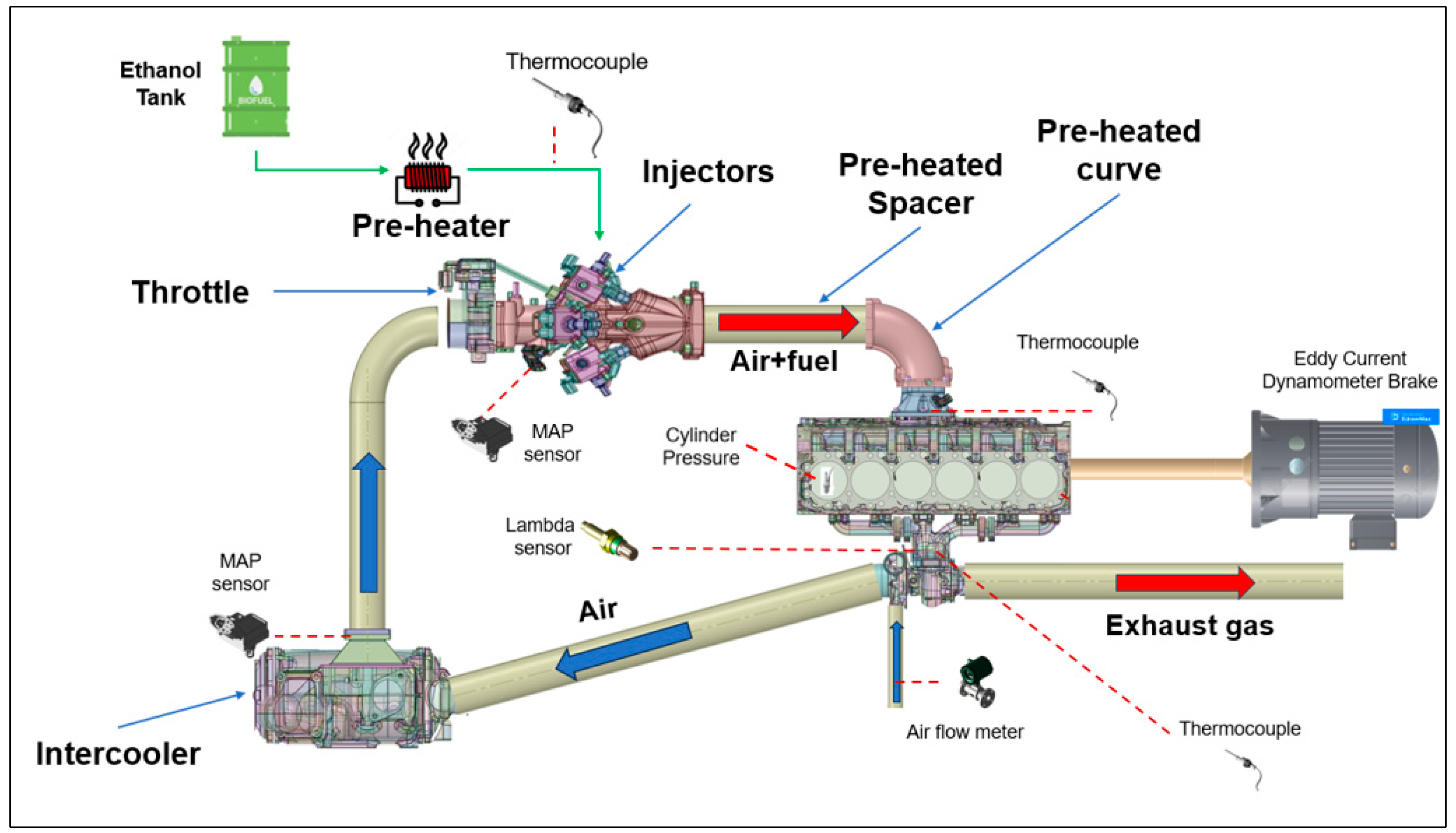
The engine under consideration is an FPT Cursor 9 SI version. The commercial version of this engine is natural gas-powered, so that some modifications were needed to operate with 100% ethanol. A schematic layout of the engine test bench is shown in Figure 1, whereas the engine specifications are reported in Table 2.

Figure 1.
Schematic layout of the engine test bench.
Table 2.
Engine specifications.
The fuel system modification regards the development of a novel single-point injection system characterized by 12 injectors mounted three by three along the circumference of the intake duct, placed sufficiently far from the intake manifold, with the main objective of enhancing the mixing between fuel and air. In addition, ethanol vaporization is favoured by pre-heating the fuel and the wall ducts. In particular, ethanol is pre-heated by hot water through a water/ethanol heat exchanger. The hot water, in turn, flows inside an external coaxial duct that covers a curved duct and a spacer, which are located downstream of the injectors, and contribute to further pre-heat the air–ethanol mixture. As the engine is turbocharged, an intercooler is included in the experimental apparatus. However, as ethanol requires a high temperature to evaporate, the operation range of the intercooler was properly managed. The intake duct was designed with a curved shape in order to reduce the system dimensions and to make the whole system compact enough to be enclosed in a box.
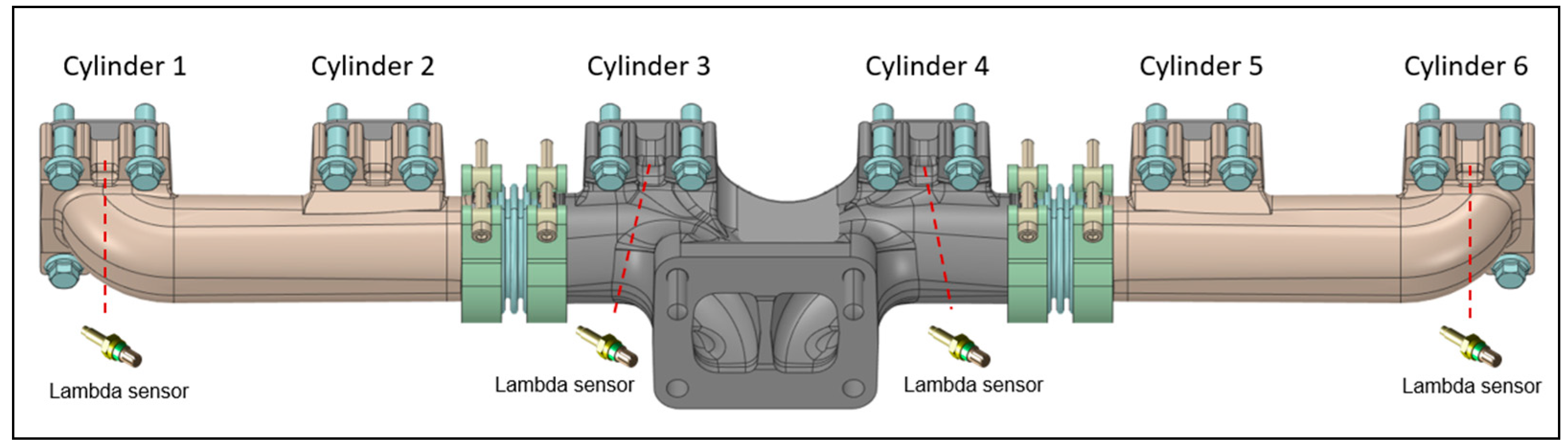
The engine was coupled with an eddy current engine torque dynamometer for measuring the brake torque and engine speed. An intake air flow meter was mounted upstream of the compressor. Two manifold air pressure (MAP) sensors were installed downstream from the intercooler for detecting the boost pressure and between the throttle valve and injectors to measure the air pressure before the injectors, while the in-cylinder pressure data were recorded using a measuring spark plug mounted only in Cylinder #1 (Figure 1). The overall air–fuel ratio was measured through a lambda sensor placed on the exhaust duct upstream of the turbine; in addition, the engine was equipped with lambda sensors arranged just upstream of the exhaust manifold for the detection of the air–fuel ratio in cylinders 1-3-4-6, as shown in Figure 2. Fuel, fresh charge, and exhaust gas temperatures were measured by means of k-type thermocouples. A detailed list of the measured parameters and the specifications of the devices used is reported in Table 3.
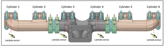
Figure 2.
Lambda sensors for measuring the air–fuel ratio in the cylinders 1-3-4-6.
Table 3.
Measured parameters and measuring device specifications.
The experimental tests performed which can provide the initial conditions of the calculation are described in the next section.
2.2. Experimental Tests
The experimental tests were carried out at low (85 kW) and medium-high (161 kW) loads obtained with 28% and 41% of WOT, respectively; based on the target application of the engine for this project, the engine speed is fixed at 1500 rpm. Before collecting any data, the engine was conditioned to ensure fully warmed and steady-state conditions. Table 4 summarizes the engine operating conditions adopted during the experimental tests.
Table 4.
Experimental operating conditions.
It is worth pointing out that the selected operating conditions represent preliminary tests to assess the reliability and stability of the engine, converted to 100% ethanol and equipped with the new injection system. For this reason, both the engine and the operating parameters are far from being optimized. This is evidenced by the λ values which indicate a rich fuel–air mixture, against the target of fuel consumption reduction. Nevertheless, the collected experimental data can be useful to preliminarily highlight the critical issues of the proposed system and to validate a CFD model helpful to describe the combustion features of ethanol as alternative fuel.
The experimental uncertainty was assessed by evaluating the repeatability of the measured data. Specifically, each test condition was repeated three times under identical operating settings. For each measured parameter, the mean and standard deviation were calculated based on the three repetitions. This statistical approach allows for the estimation of the experimental error due to random fluctuations and minor variations in boundary conditions, providing a direct measure of the repeatability of the experimental setup.
The recorded experimental data are summarized in Table 5 and Table 6 for the Low and Medium-high load, respectively. The tables include the engine performance in terms of brake parameters and indicate mean variables and their standard deviations.
Table 5.
Measured parameters at Low load: mean and standard deviation values.
Table 6.
Measured parameters at Medium-high load: mean and standard deviation values.
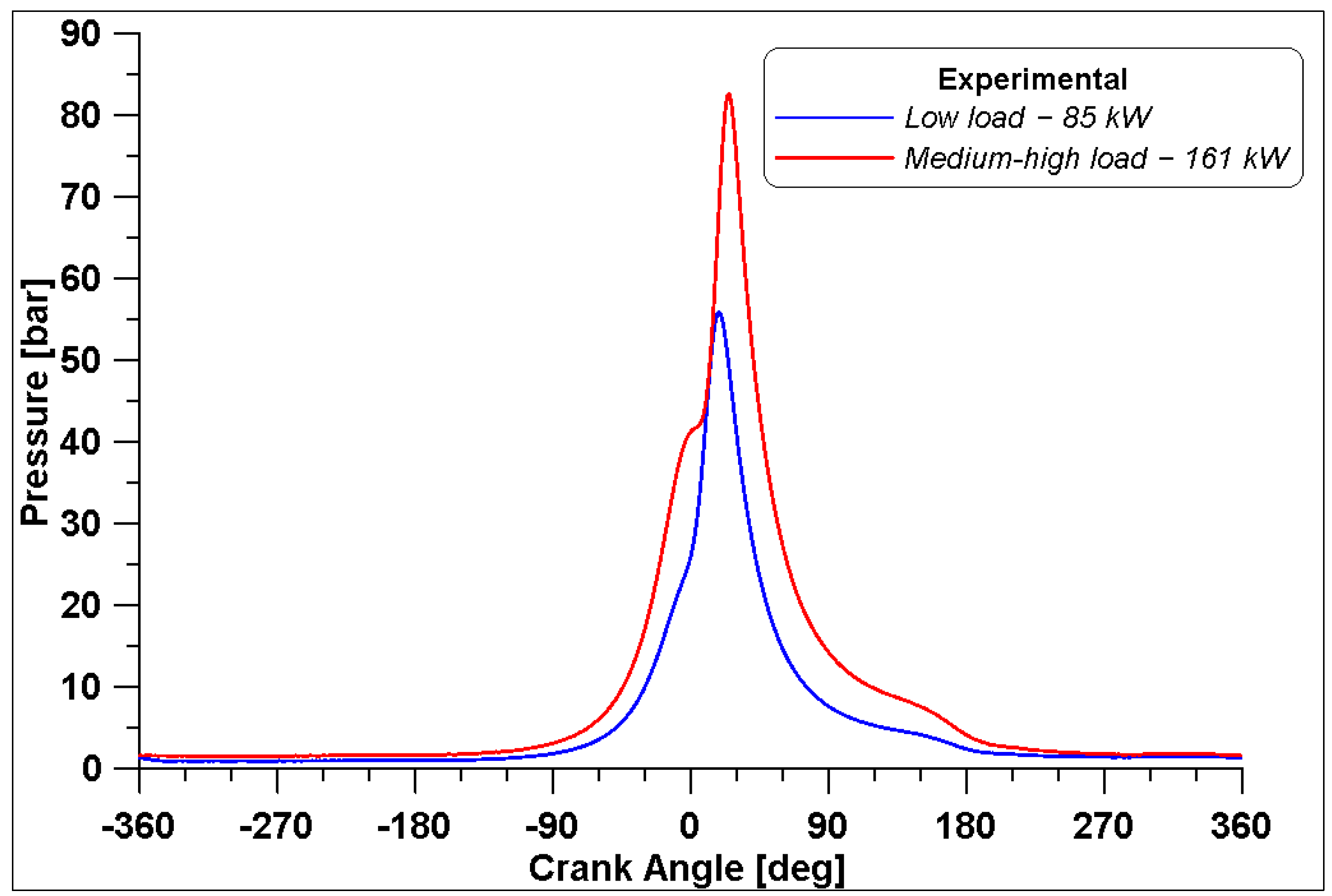
The in-cylinder pressure was measured with a measuring sparkplug only in Cylinder #1 for both operating conditions, and the average curves over 250 cycles are reported in Figure 3 for 85 kW and 161 kW.

Figure 3.
Measured in-cylinder pressure at two different loads.
As observed in Table 4, the different values of boost pressure lead to different air supply of the engine with consequent different compression curves. The maximum in-cylinder pressure inside Cylinder #1 is 55.9 bar for the low load case and it occurs at 18° ATDC, while the maximum pressure for the medium-high load is 82.5 bar at 25° ATDC. It must be noted that, due to the high-pressure level achieved for the medium-high case to prevent knock occurrence, the spark timing is set to 5° BTDC, which means it is delayed with respect to the low load case. Relatively low COV IMEP values of 1.63% and 1.64% were calculated for low load and medium-high load cases, respectively.
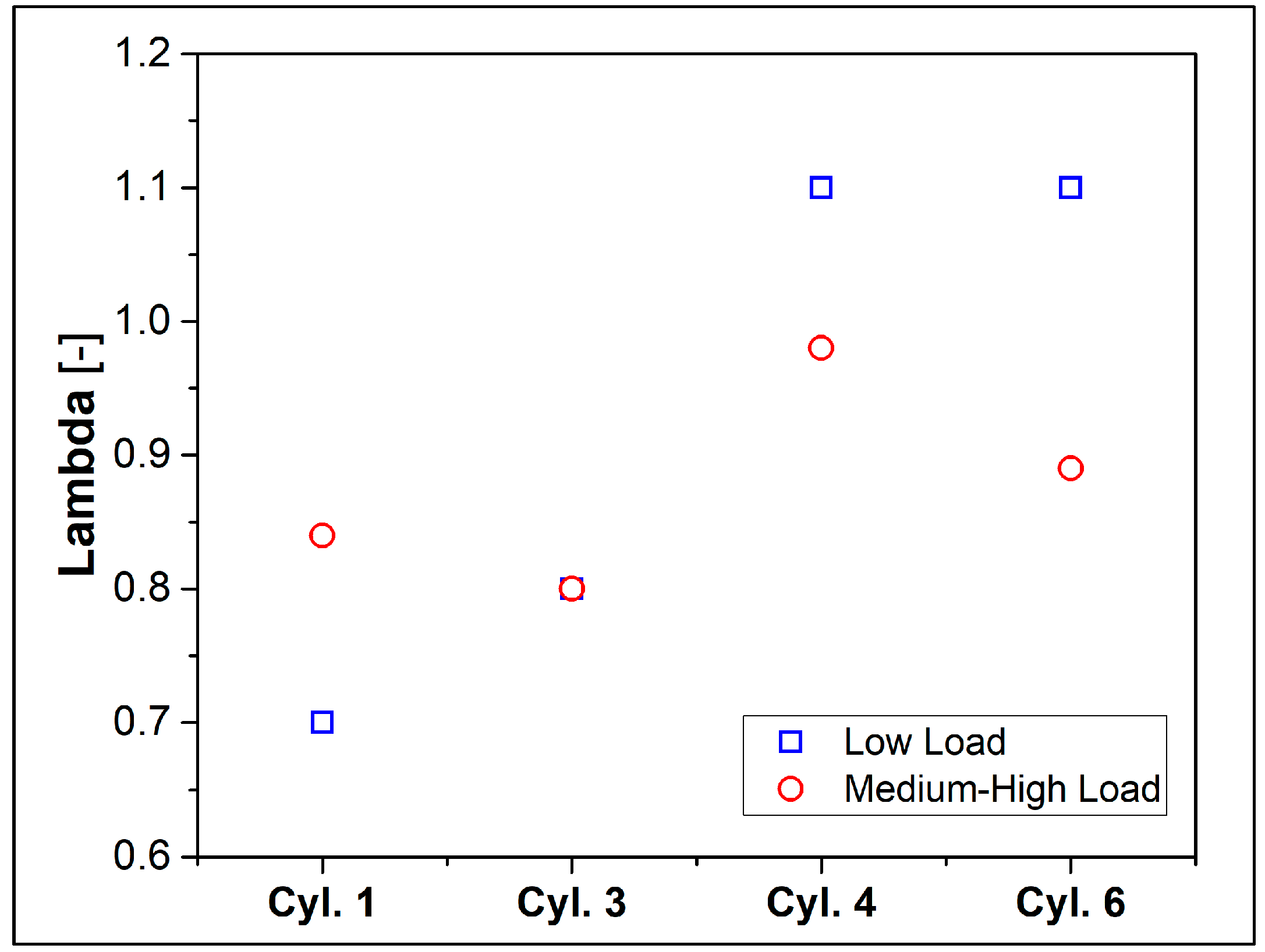
One aspect that deserves particular interest is the non-uniformity (maldistribution) of the mixture between the cylinders. This undesirable phenomenon is shown in Figure 4, in which the lambda values are plotted for each cylinder equipped with a lambda sensor. As already pointed out, the overall mixture features a rich fuel–air ratio. However, this situation becomes more critical in Cylinders #1 and #3 while the cylinders arranged diametrically opposite to the intake manifold (Figure 1), i.e., #4 and #6, can achieve higher air-to-fuel ratios, closer to stoichiometric value or typical of lean operation.
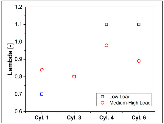
Figure 4.
Measure of the lambda over the cylinders.
However, this non-uniformity of the mixture will be considered as it could lead to incomplete combustion, especially if the local mixture is too rich or too lean, and it can play a crucial role in the unburned hydrocarbons and carbon monoxide emissions.
3. Numerical Simulation Setup
CFD represents a fundamental tool for the prediction of the in-cylinder phenomena especially when innovative fuels are introduced [37,38]. The computational activities were carried out to examine the in-cylinder combustion process and to explore the main characteristics of the ethanol-fuelled engine in terms of performance and pollutant formation.
The computational results were obtained by using the 3D code ANSYS Forte® and they refer to the set of experimental data at the operating conditions shown in Table 4. To this purpose, based on the geometry provided by the manufacturer, the computational closed valve domain was created for a 30° degrees sector including only the bowl, the head, and the cylinder liner (Figure 5).

Figure 5.
30° sector of cylinder geometry.
Generally, the initial calculation conditions were assigned at a crank angle within the closed valve period (132° ATDC) in accordance with data of the experimental campaign. Pressure is directly retrieved from experimental measurements while initial temperature is calculated to match the same measured trapped mass, considering the mass flow rate in Table 4.
Regardless, one of the main challenges to build a reliable model is the choice of the kinetic mechanism; especially when it aims at describing the combustion development of an innovative fuel. In this regard, five chemical kinetic mechanisms for ethanol oxidation were tested. All simulations are performed considering the initial condition in Table 7. Given the absence of the intake and exhaust duct domains and the valve lift movements, the mass exchange phase cannot be simulated. To characterize the initial flow field, a swirl ratio equal to 1 is assigned.
Table 7.
Simulation initial conditions.
The five kinetic mechanisms are listed in Table 8; the first two rows display the number of species and reactions since a more detailed and complex chain of reaction is expected to increase the computational efforts. In this regard, Table 8 includes the computational times required for the entire simulation and the time dedicated specifically to chemistry; the choice of the kinetic mechanism is also influence by this aspect. Naturally, to this aim, a reduced mechanism is considered reliable if it can provide the same results as a more detailed one. In Table 8 the main results in terms of performance and combustion characteristics are reported as well.
Table 8.
Ethanol fuel kinetic mechanisms and computational results.
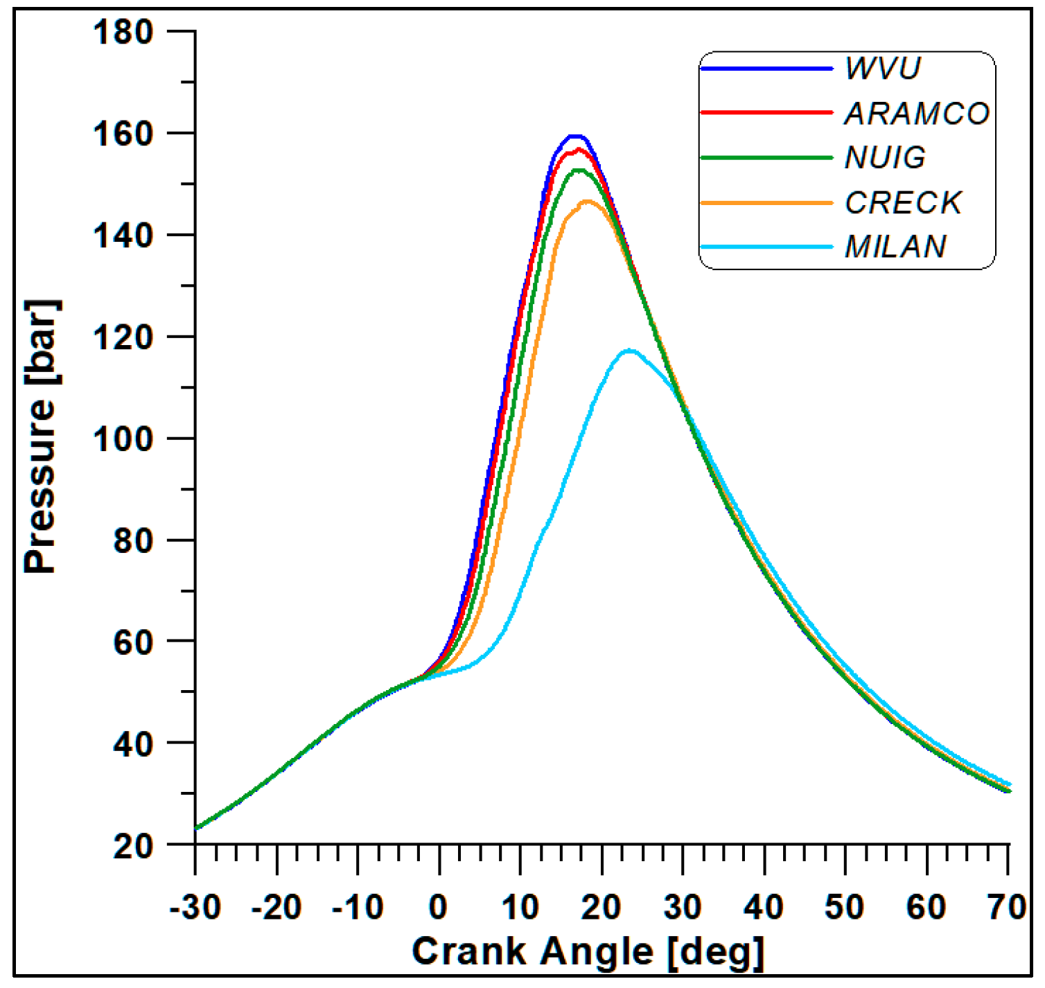
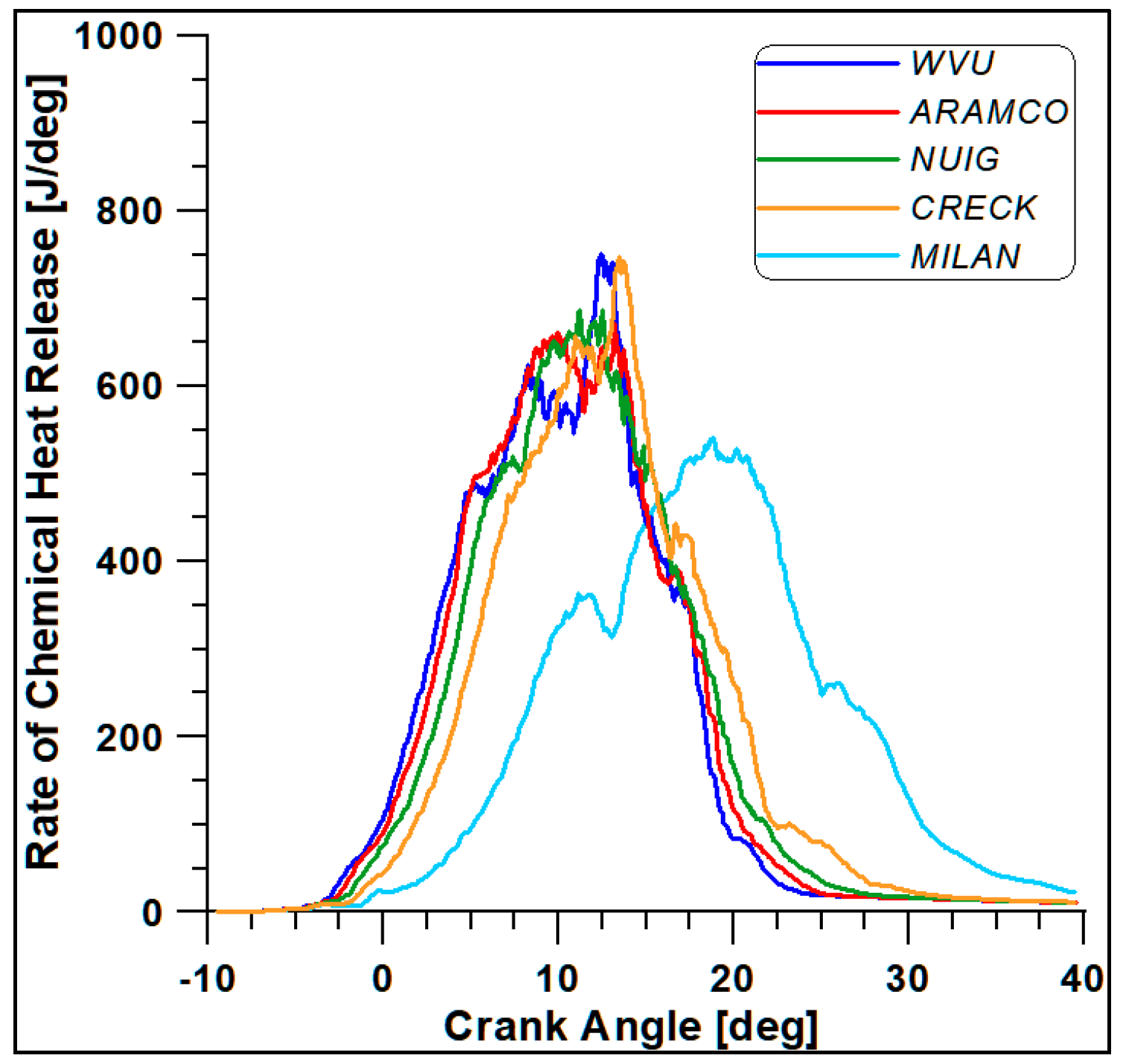
The first four mechanisms (WVU, ARAMCO, NUIG, and CRECK) provide almost similar results, while the fifth scheme (Milan-Merino) considerably differs from the others. Such a conclusion is confirmed by Figure 6 and Figure 7, where the in-cylinder pressure and rate of heat release (ROHR) display the overall combustion development described by the different oxidation mechanisms.
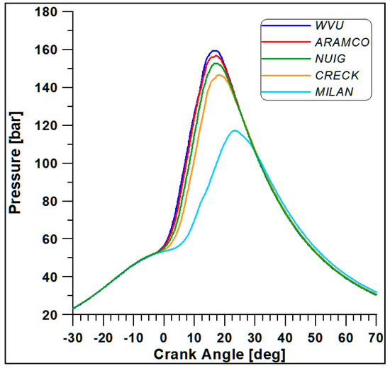
Figure 6.
In-cylinder pressure with different kinetic mechanisms.
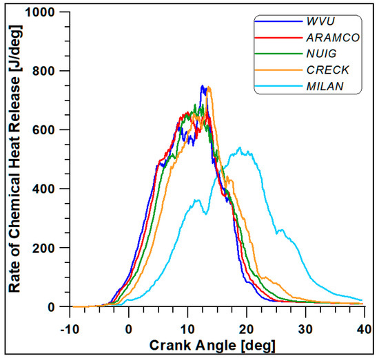
Figure 7.
Rate of heat release with different kinetic mechanisms.
Based on the computational costs and overall outcomes from this preliminary analysis, the WVU mechanism appears to be suitable for faster calculations, while the NUIG (Mech1.1), which includes a sub-mechanism for C2H5OH validated for high pressure values [43], provides the best compromise between accuracy and computational cost [44]. This mechanism also includes reactions for the NO and NO2 formation.
Mesh Sensitivity Analysis
Once the kinetic mechanism (WVU) is selected, in a second step, a mesh sensitivity analysis is performed to optimize the computational time and to ensure the reliability of the results. Six computational grids with different resolutions were built by using the Forte® sector mesh generator, and in Table 9, the number of cells and sizes are reported together with computational times. Simulations are performed on a workstation equipped with a 13th Gen Intel® Core™ i9-13900 2.00 GHz processor, 64 GB of RAM, a 64-bit operating system, and a total of 24 physical cores and 32 logical processors.
Table 9.
Mesh dimensions.
This analysis is performed by simulating the previous test case but using grids with different resolutions and assessing the variations of in-cylinder trends and overall results.
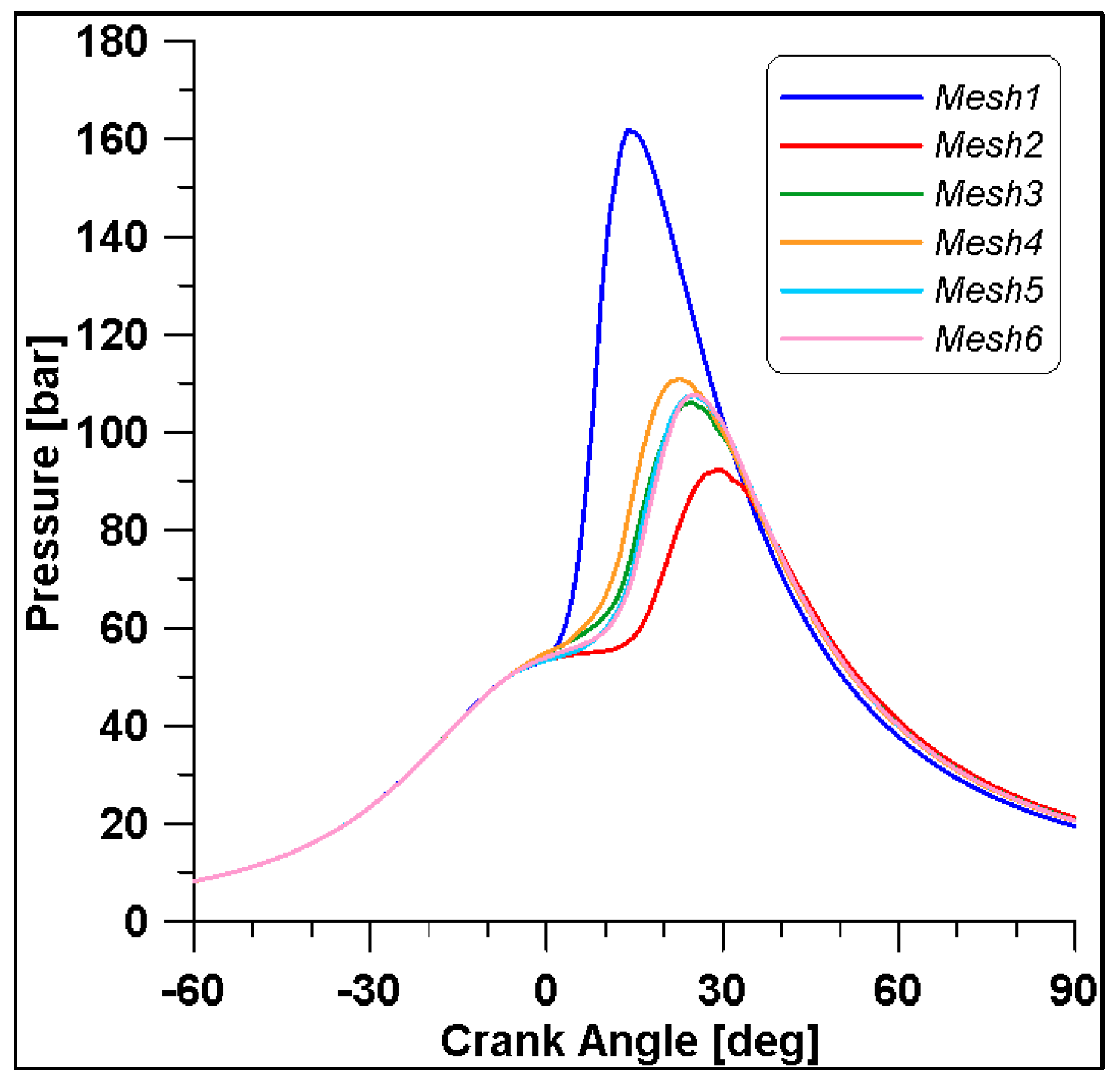
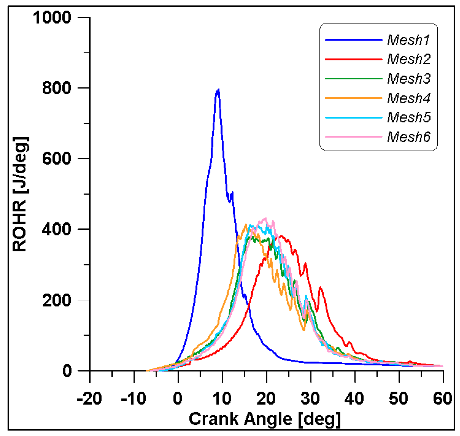
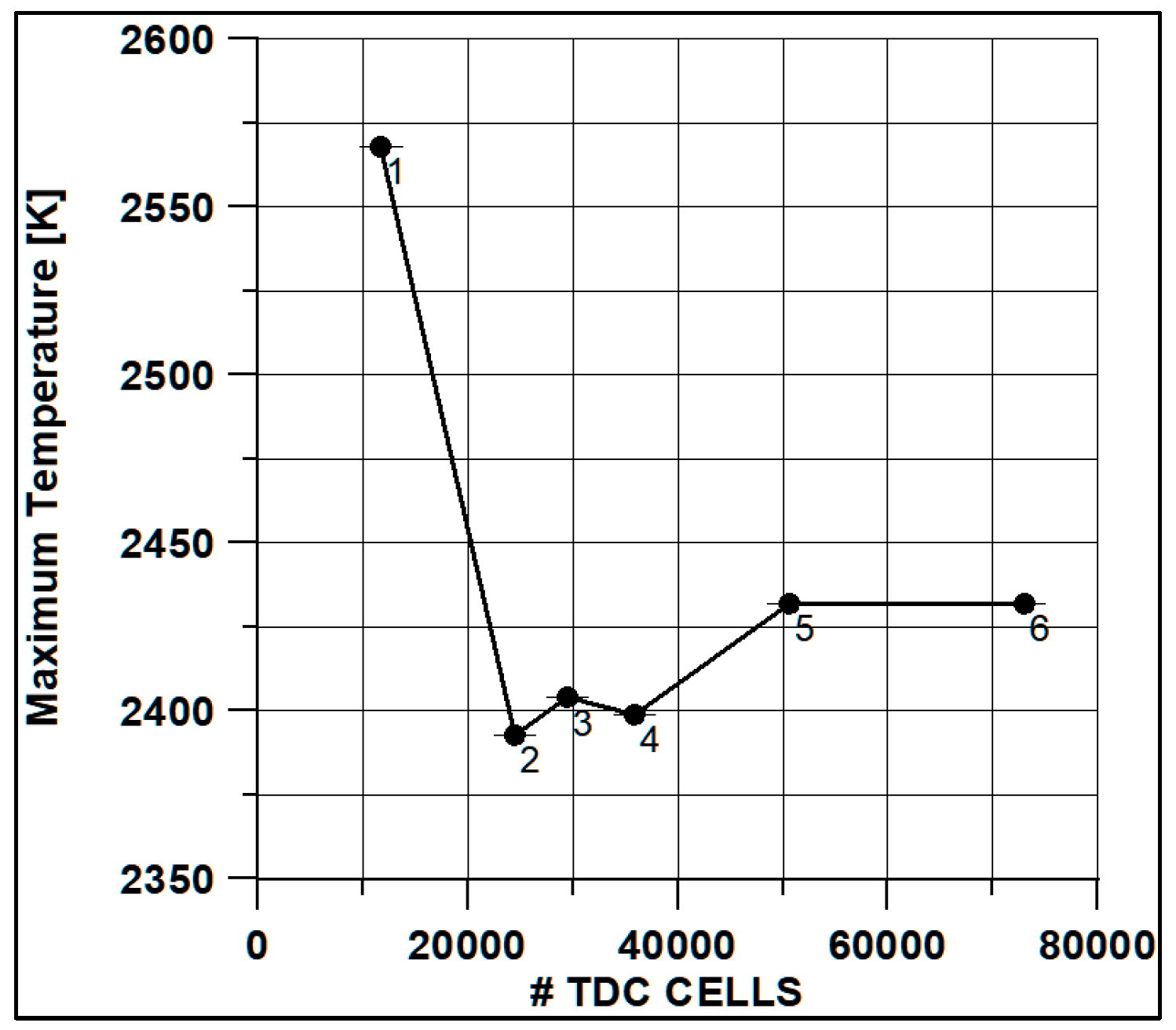
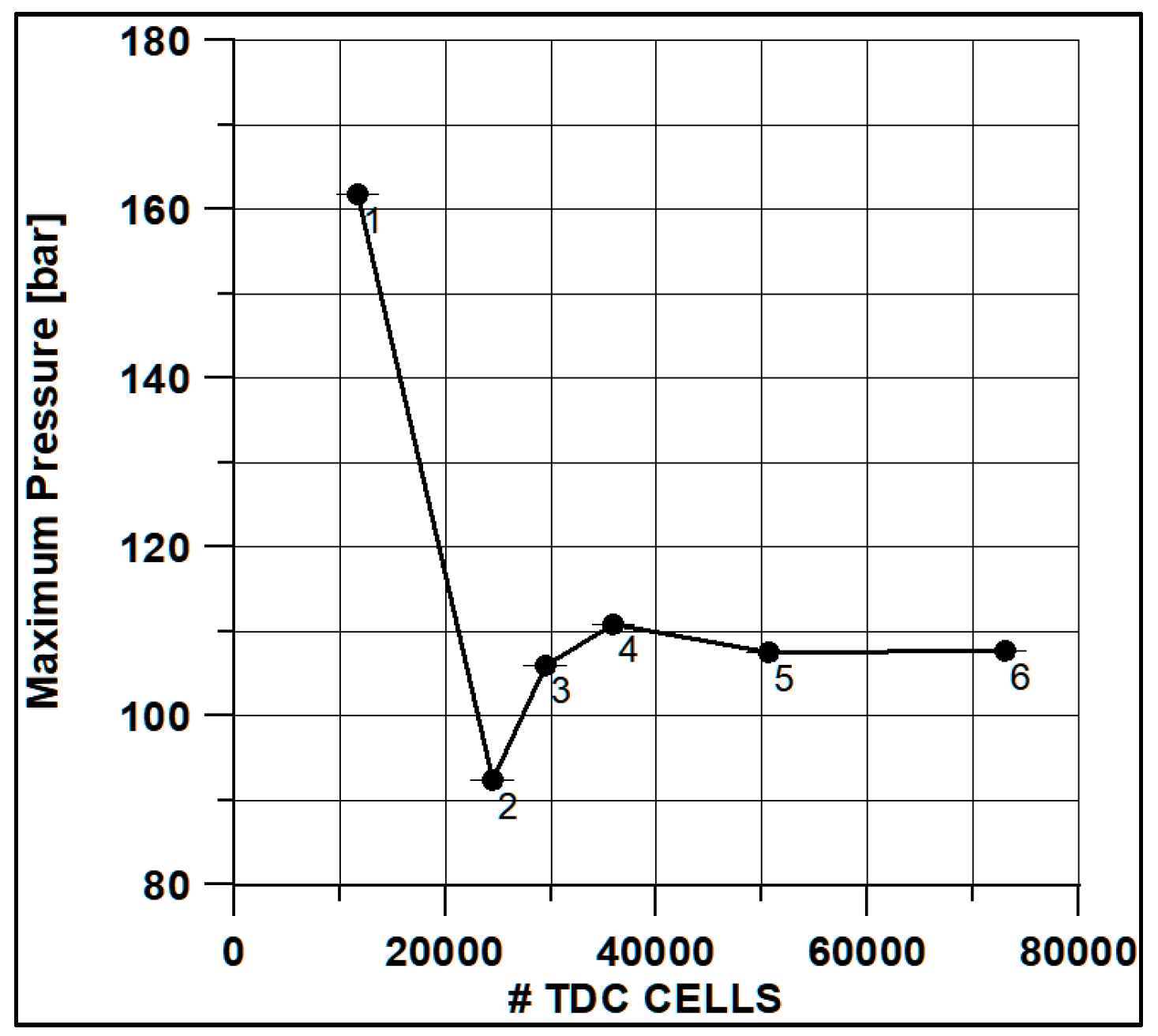
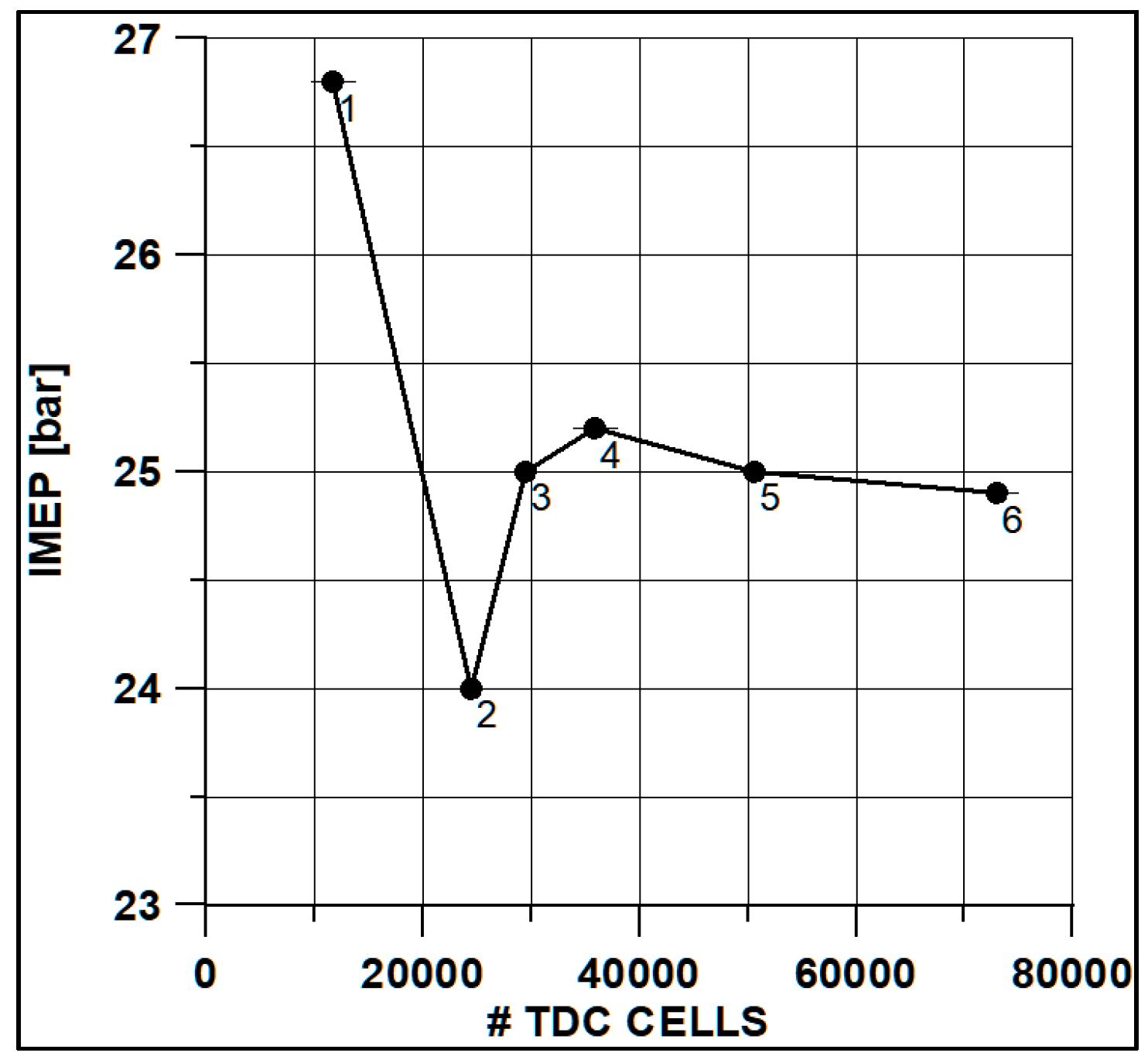
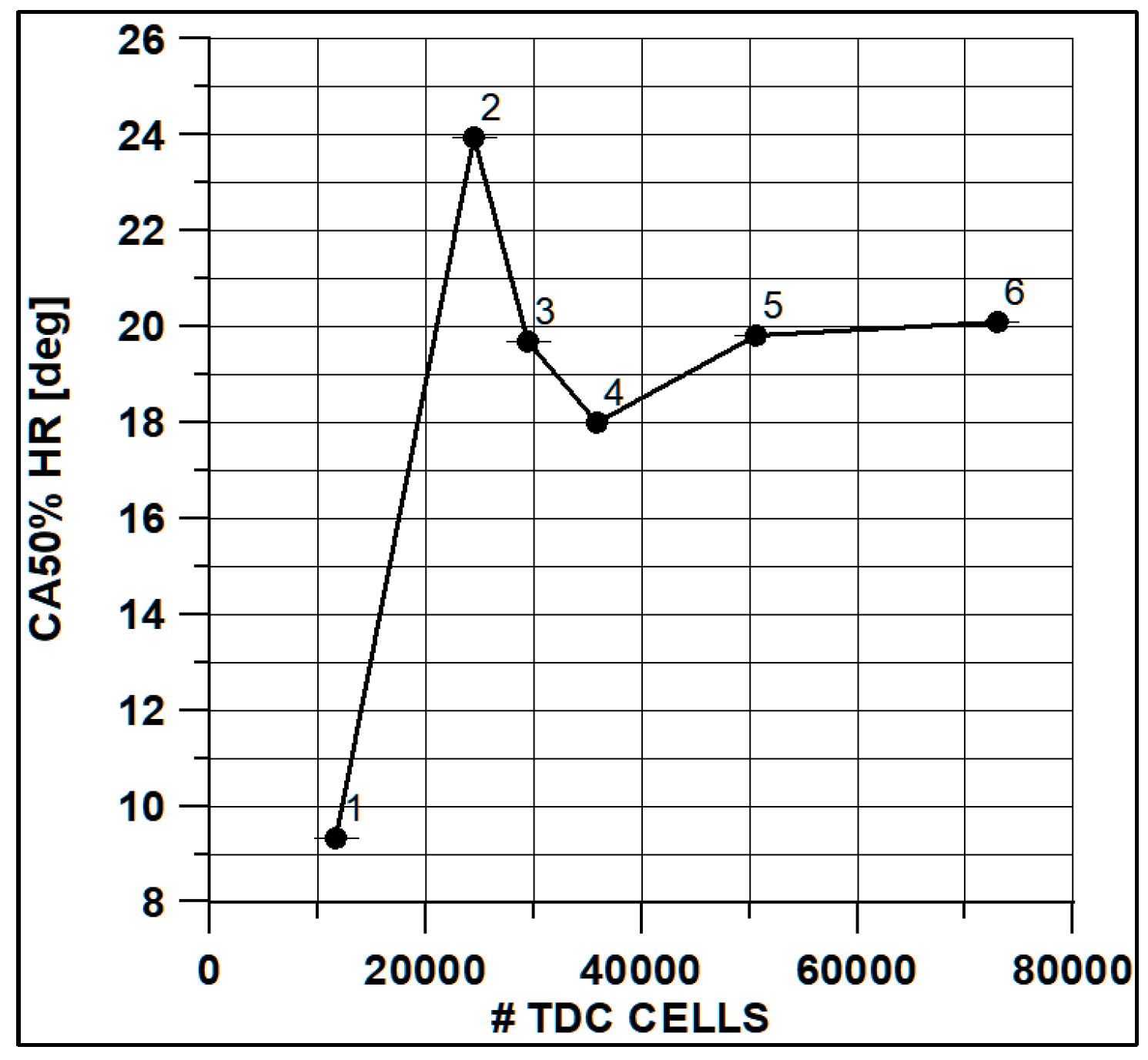
In Figure 8 and Figure 9, the results of pressure and ROHR show the sensitivity to the grid size. As displayed in the figures, the results of the coarsest grids (Mesh #1 and #2) present remarkable differences from the other ones, both in terms of pressure curves and heat release development. In Figure 10, Figure 11, Figure 12 and Figure 13, several characteristic engine parameters (i.e., IMEP, pressure, and temperature peaks, and crank angle at 50% of heat release) are reported as a function of the number of bowl cells in the six computational meshes. As mentioned above, coarser meshes lead to significant deviations from the results at grid convergence. The three finest meshes (Mesh #4, #5, and #6) reproduce quite similar results for each property considered. Nevertheless, to ensure the convergence of the results and to account for an acceptable computational time, Mesh #5, illustrated in Figure 14, is chosen for the next CFD calculations. The 30° sector grid features about 170,000 cells at IVC and 50,000 cells at TDC.
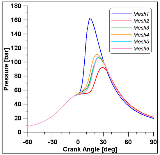
Figure 8.
In-cylinder pressures for different grid sizes.

Figure 9.
ROHRs for different grid sizes.
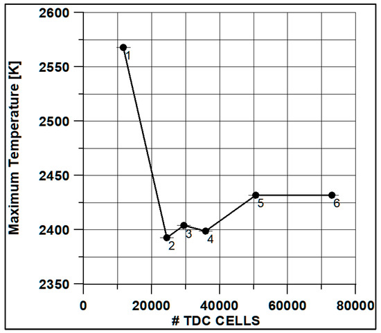
Figure 10.
Max temperature vs. cells number at TDC.
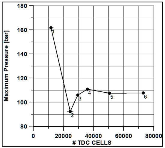
Figure 11.
Max pressure vs. cells number at TDC.
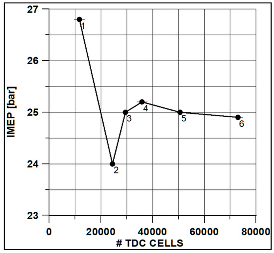
Figure 12.
IMEP vs. cells number at TDC.
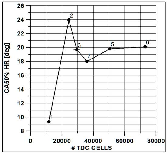
Figure 13.
Crank angle at 50% of HR vs. cells number at TDC.
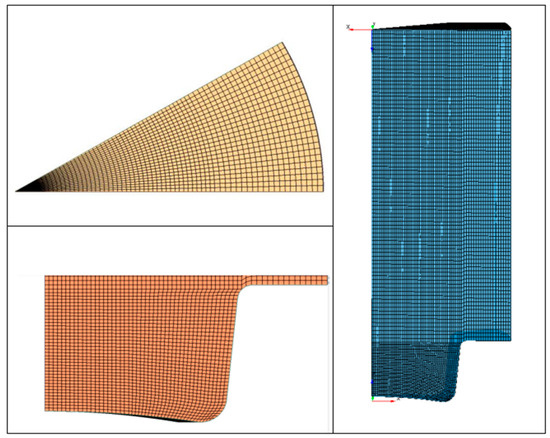
Figure 14.
Representation of Mesh#5.
4. Combustion Analysis and Experimental Validation
In this section, based on the experimental indications obtained from the engine at test bench (Cylinder #1), the numerical models developed for the study of ethanol combustion and pollutant formation are validated. It is worth mentioning that the experimental data do not provide information on combustion effectiveness and polluting emissions, but both global measurements and in-cylinder pressure are useful for validation purposes.
4.1. Combustion Modelling
As anticipated in Section 1, the validation of the CFD was carried out considering the λ value of the sole cylinder equipped with a pressure transducer (#1); subsequently, a comparison with the computations considering the λ of the cylinder featuring the best fuel supply, i.e., #4/6 for low load and #4 for medium-high load (see Figure 4) allowed for observing how the different air-to-fuel ratios affect the performance of the entire engine.
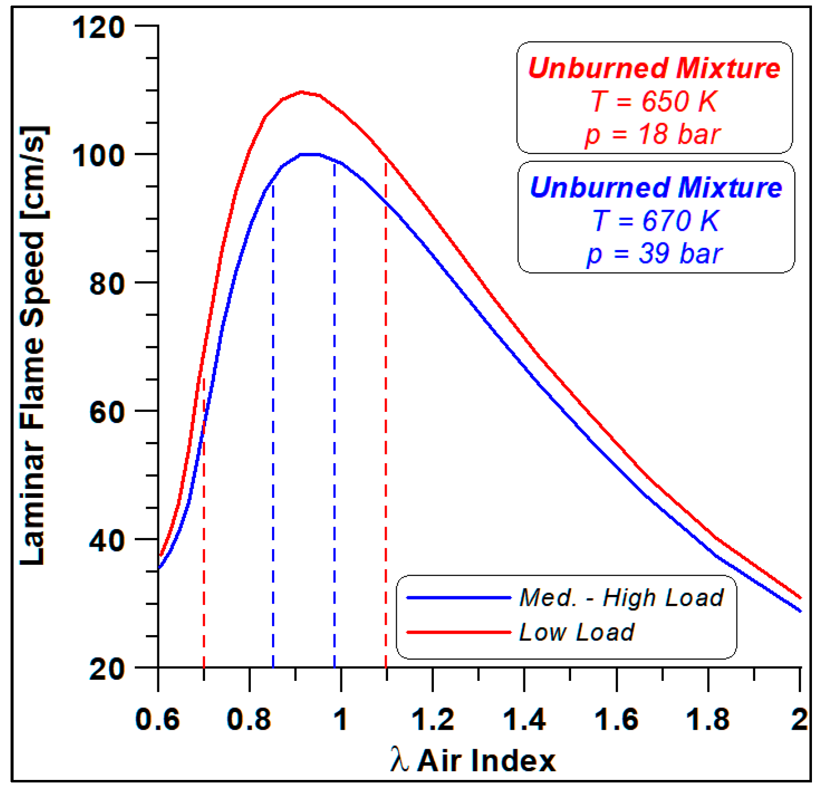
Firstly, the WVU mechanism is employed in the Chemkin environment for a first estimate of the laminar speed at the thermodynamic conditions of an ethanol–air unburned mixture close to spark-ignition events. Figure 15 displays the laminar flame speed (LFS) trends as a function of the air index (i.e., the inverse of fuel/air equivalence ratio).

Figure 15.
Ethanol laminar flame speeds at low and medium-high load spark conditions.
The curves refer to the two different load conditions, and the cylinder-to-cylinder shift of air index level is also displayed, that is, for each load, the dashed lines detect the LFS at the considered λ. Mainly in the low-load case, significant variations in flame speed are expected together with enhanced differences in NOx formation.
The CFD calculations are still performed with the ANSYS Forte® code using the models listed in Table 10 and by using the WVU kinetic mechanism, which is selected for an acceptable compromise between accuracy and computational costs. Based on the results obtained and reported in the previous section, for this analysis, this choice allows a faster assessment of the model constants to meet the experimental pressure curves. As previously stated, in a second phase, the NUIG mechanism will provide information about pollutant formation and contents at EVO.
Table 10.
CFD models.
For CFD simulation purposes, the full laminar flame speed library included in the ANSYS Forte® package is accessed. The simulation of the real flame propagation process, based on turbulent flow features, relies on the evaluation of the turbulent-to-laminar flame speed ratio and of a progress variable (G scalar function) [45]:
- -
- The turbulent-to-laminar flame speed ratio depends on the following relationship:
- -
- The G function allows the identification of the current location of the flame front and the G-equation model consists of a set of Favre-averaged equations as implemented in ANSYS Forte [47]:
4.2. Test Cases of Closed Valve Engine Simulation
The performed calculations refer to the two experimental cases described in the previous section, and they will be referred to as “Low load” and “Medium-High load”. As already evidenced by looking at Table 4 and Figure 4, both cases are characterized by a reach mixture (i.e., air index λ = 0.7 and 0.84, respectively) and strong disuniformity in fuel/air mixture among the cylinders. Therefore, the data available from Cylinder#1 (the only one equipped with pressure transducers) are used for the validation of the CFD model. However, a relevant production of carbon monoxide is expected due to the oxygen lack in the mixture. Conversely, the same Figure 4 shows that in the low load case, a maximum λ value of 1.1 is detected in cylinders #4 and #6 while at medium-high load conditions, a maximum air index of 0.98 is obtained in cylinder #4.
For this reason, a comparison of the two limit conditions is carried out to highlight the differences in terms of performance and emissions related to the different development of combustion processes and flame speed, as evidenced in Figure 15.
5. Results and Discussion
5.1. Low Load Case (85 kW)
The operating conditions investigated are shown in Table 4, related to the experimental low load (85 kW) test case. The analysis aims at validating the models by comparing numerical results with available experimental data. As stated, a more comprehensive description of the combustion development and noxious species formation is also addressed.
Since the CFD calculations are currently carried out in the closed valve period, the in-cylinder initial conditions should match the experimental information in terms of total trapped mass and fuel/air ratio. Consequently, while initial pressure and mixture composition are assigned, the temperature is calculated. A first trial value of 317.37 K allows a good approximation of the air trapped mass (1.523 g), and the lambda level is fairly preserved (λ = 0.72) referring to the first cylinder.
Particular attention should also be paid to the flame propagation modelling (Equations (1) and (2)) and therefore a sensitivity analysis has been carried out by varying the initial conditions of turbulent parameters, which are unknown when working with closed valve geometry.
Therefore, four preliminary test cases are carried out to analyse the combined effect of the initial TKE and the b1 factor (Equation (2)). It should also be observed that the first choice of initial conditions allows both trapped mass and mixture composition to be approached, but it also leads to an overestimation of the fuel mass with respect to the average experimental value. So, two additional test cases are performed by reducing the total trapped mass with the same lambda value, via an increased value of the temperature at the initial crank angle (344 K). In Table 11 the performed test cases setups are outlined. The variation of the TKE and b1 parameters induces great modifications to the combustion development and the pressure and ROHR evidence a non-linear trend with the TKE.
Table 11.
Case setup for CFD validation.
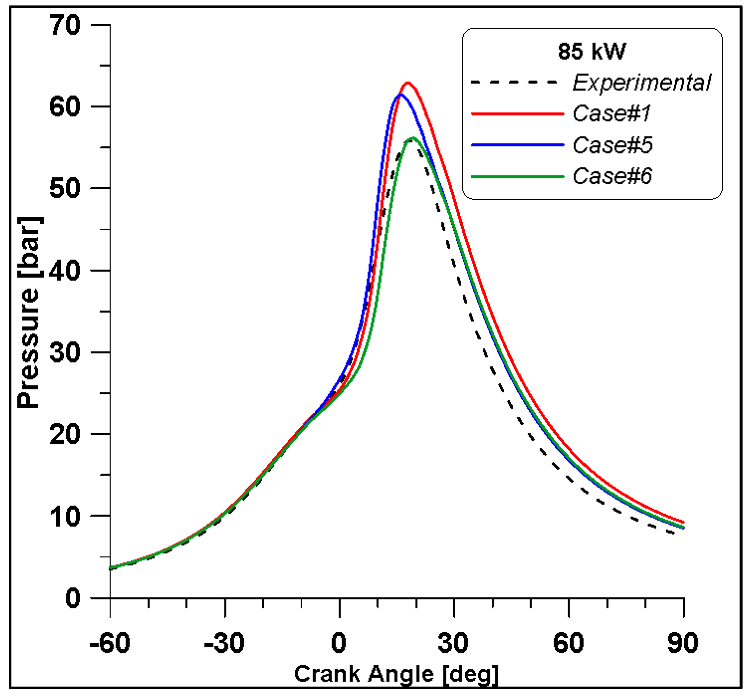
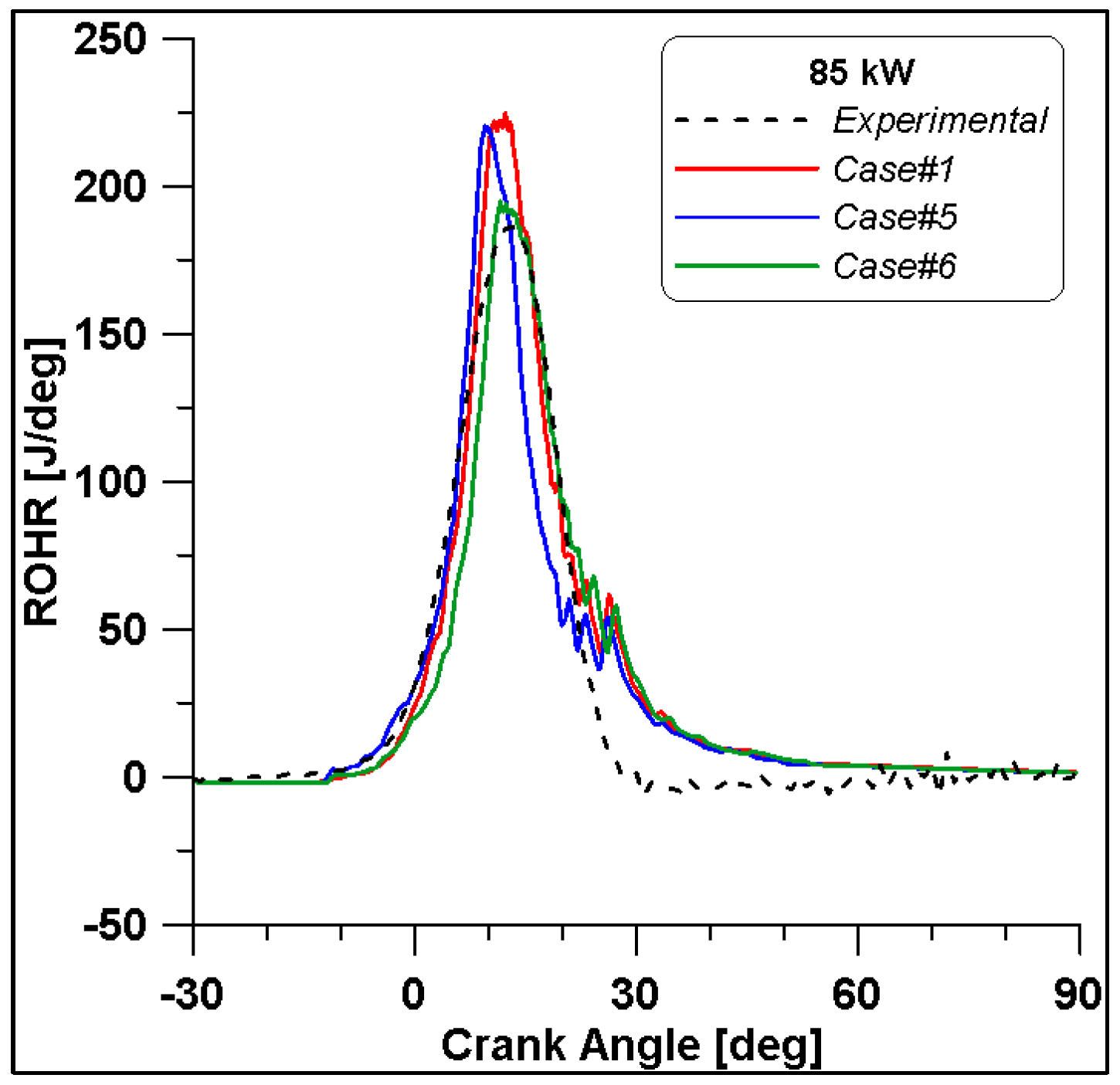
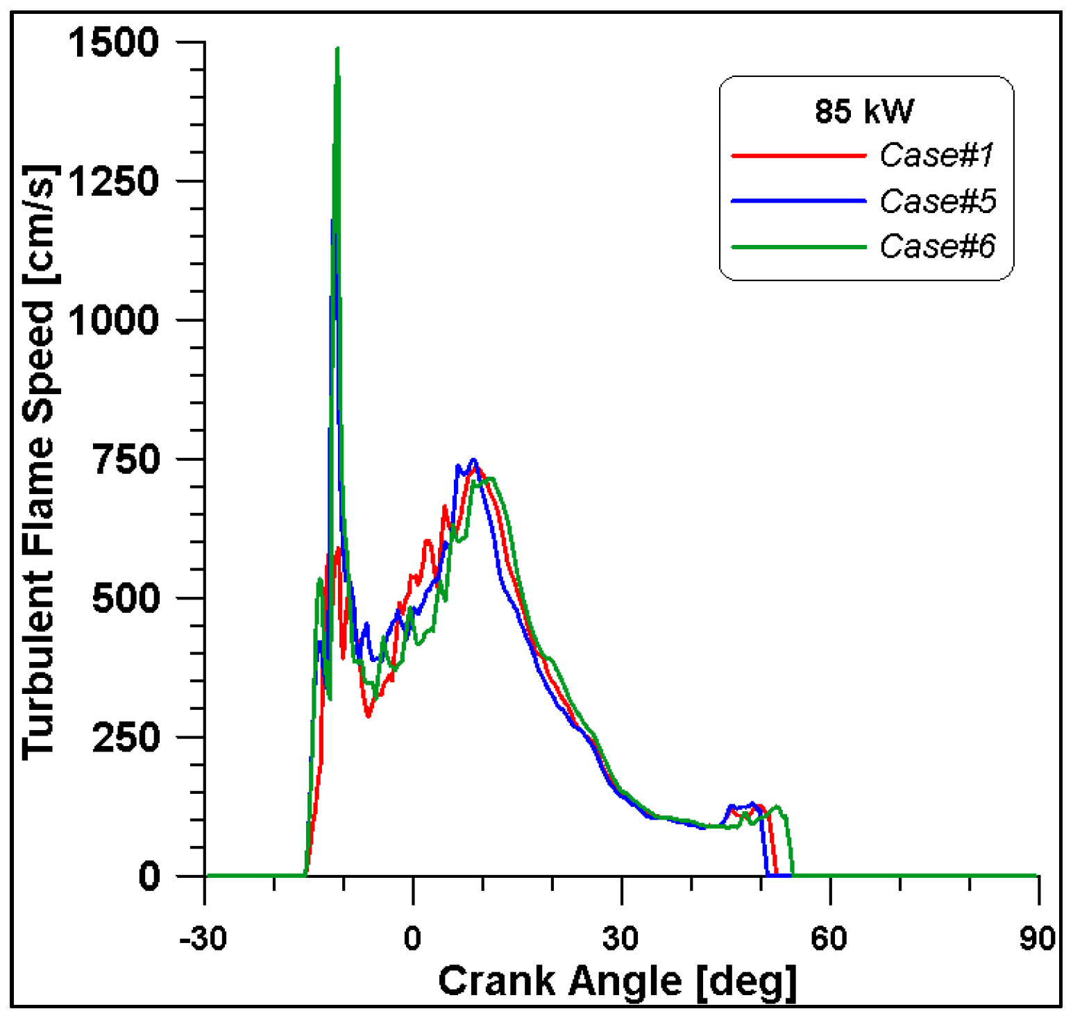
Figure 16, Figure 17, Figure 18 and Figure 19 display in-cylinder pressure, ROHR, laminar flame speed, and turbulent flame speed for Cases #1, #5, and #6 and a slight decrease in pressure and combustion duration is observable. Cases #5 and #6 feature a reduced mass of fuel (Table 11), but the lambda value is the same. In addition, focusing on Case #6, it is possible to conclude that the b1 factor plays a fundamental role in the flame propagation and combustion development. Indeed, a decreased value of 2.85 (Table 11) allows a good fit of the experimental results, achieving the same peak of pressure at the same crank angle and combustion duration. Furthermore, the laminar flame speed shows a slight enhancement for Cases #5 and #6 since it is a function of temperature and mixture composition, and only the former is varied. Apart from the first strong peak, the turbulent flame speed also undergoes the effects of b1 reduction evidenced by the lowest value observed across the TDC in Case #6.
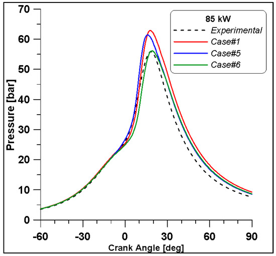
Figure 16.
In-cylinder pressure for cases #1, #5 and #6.

Figure 17.
Rate of Heat Release for cases #1, #5 and #6.
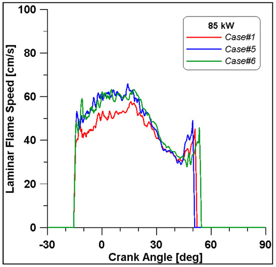
Figure 18.
Laminar flame speed for cases #1, #5 and #6.
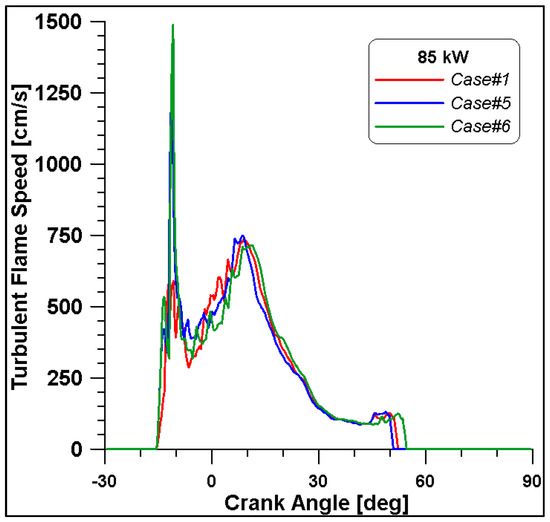
Figure 19.
Turbulent flame speed for cases #1, #5 and #6.
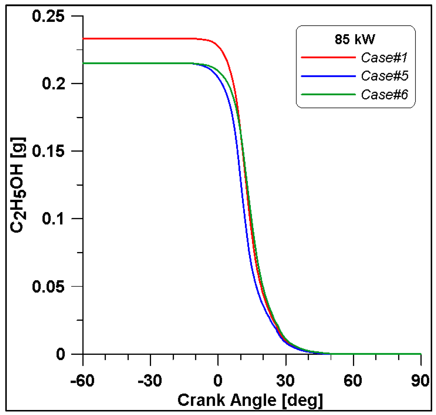
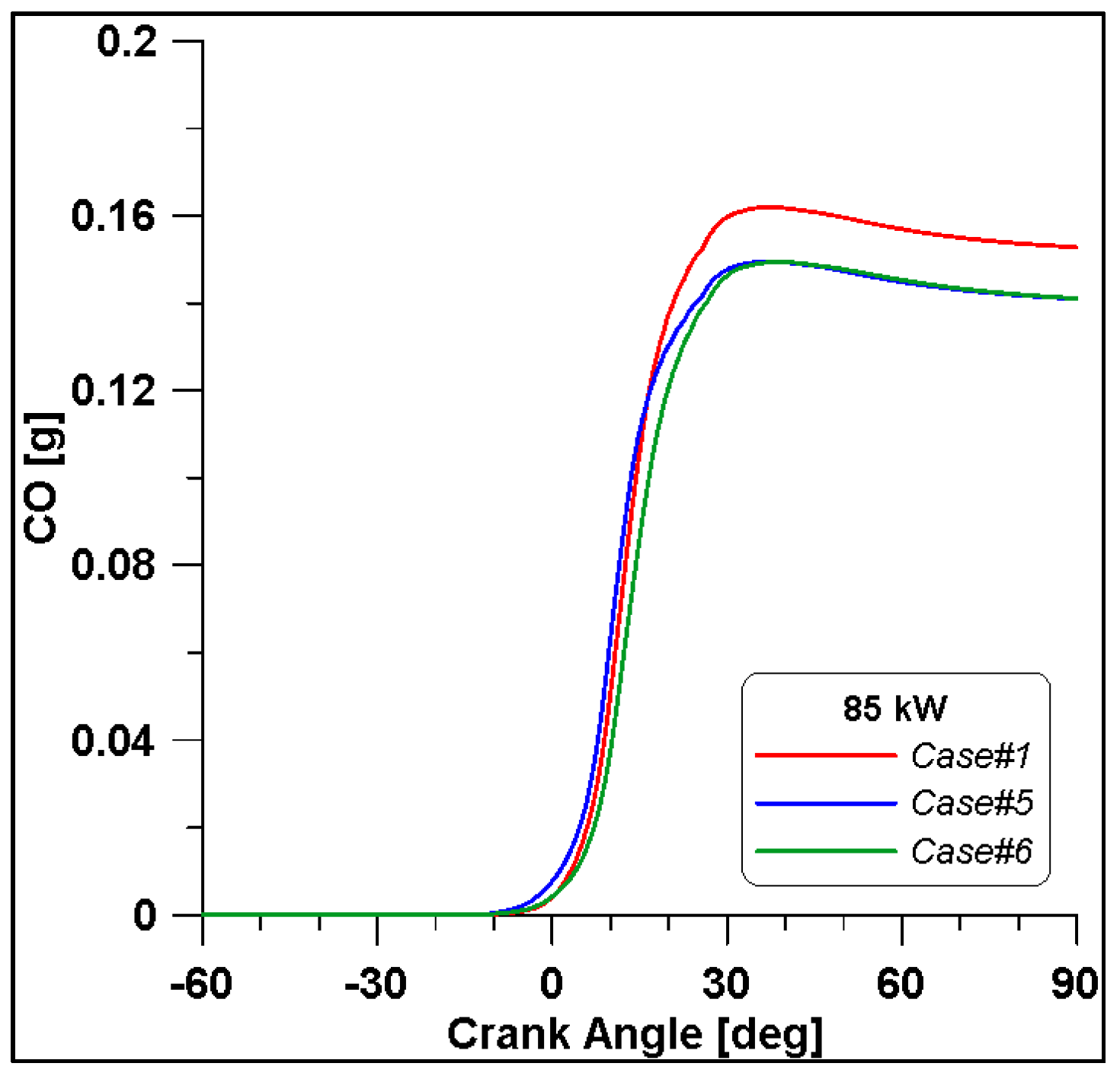
By looking at the ethanol mass trend in Figure 20, in Case #1, the initial value is higher than the other two. In any case, the rate of consumption follows a similar trend. As expected, lower CO emissions are reached at the end of combustion due to the reduced fuel mass introduced in the cylinder for Cases #5 and #6 (Figure 21).

Figure 20.
Ethanol mass trend for cases #1, #5 and #6.
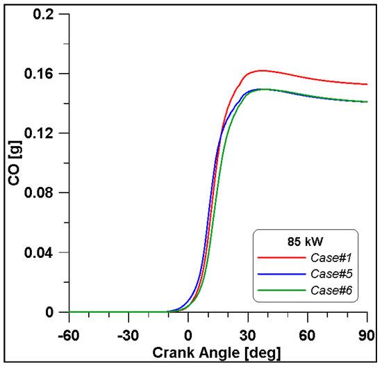
Figure 21.
CO mass trend for cases #1, #5 and #6.
It is interesting to notice that both laminar and turbulent flames in Figure 18 and Figure 19 appear to extinguish at nearly 50° ATDC; yet in Figure 21, a continued reduction of CO beyond this crank angle is shown. Since ethanol consumption is completed (Figure 20), it is evident that reaction activity not linked to the flame propagation is still occurring.
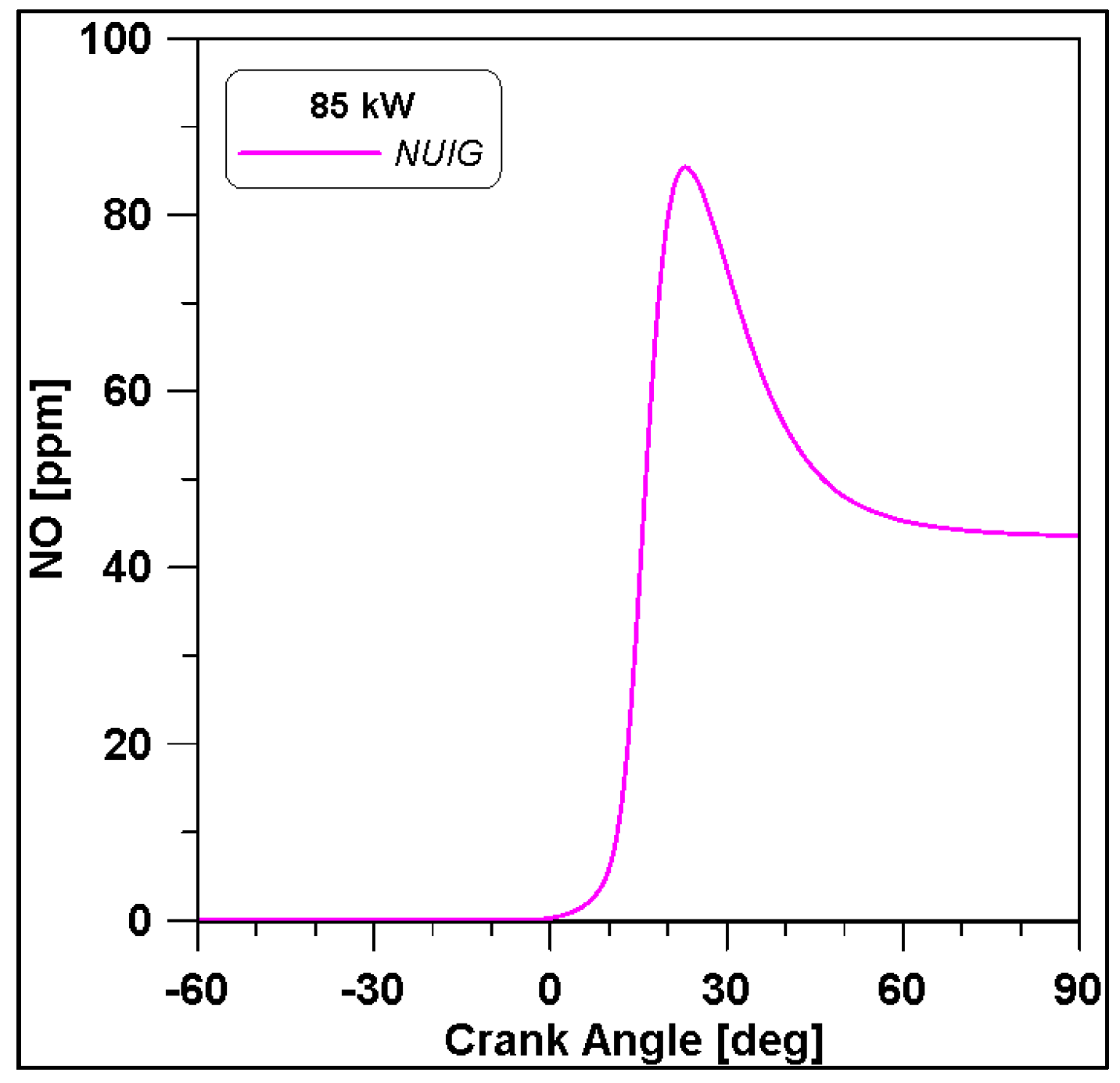
Based on the presented results, Case #6 represents the best experimental pressure data fitting. Therefore, this case is performed including the NUIG kinetic model both for an additional validation and for NOx species evaluation. Pressure results in Figure 22 demonstrate a perfect overlap with the WVU mechanism confirming the reliability of the WVU mechanism. In Figure 23 a first quantification of NO emissions is shown.
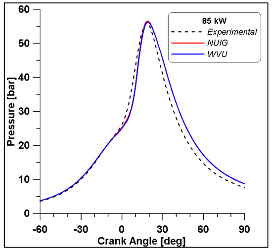
Figure 22.
Comparison between WVU and NUIG mechanisms.
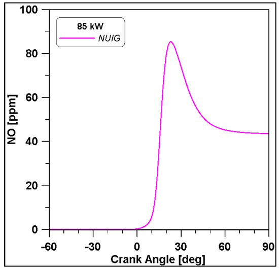
Figure 23.
NO emissions for cylinder#1. NUIG mechanism.
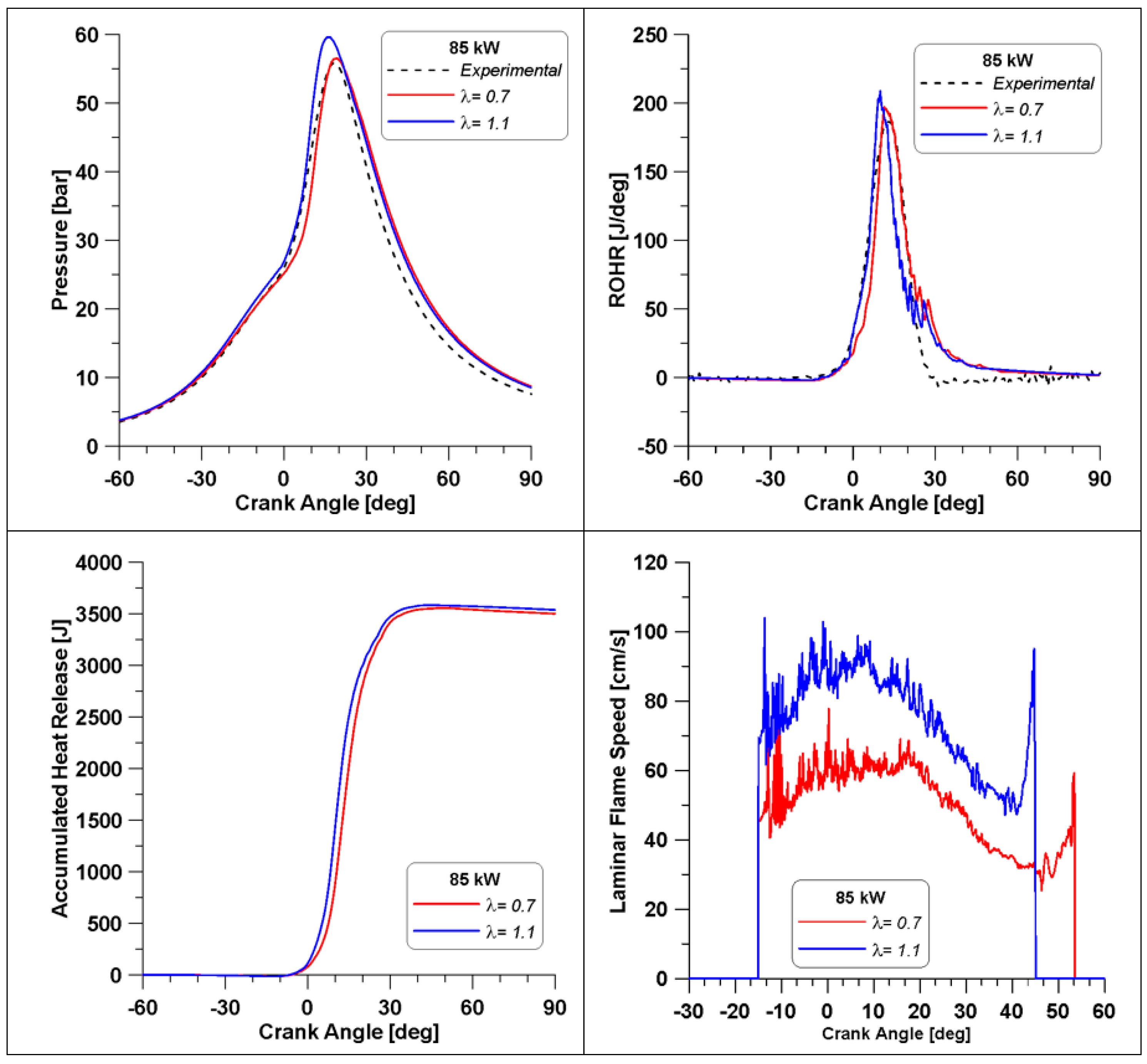
In Figure 24, a comparison between the combustion parameters for the two extreme conditions (λ = 0.7 and λ = 1.1) is reported. The λ value of 1.1 is achieved by reducing the mass of fuel. The experimental curve is displayed as well, recalling that it refers to λ = 0.7. The enhancement of the λ value leads to increased and anticipated peaks of pressure and of ROHR. This can be attributed to two factors: the first one is represented by the higher presence of oxygen that also facilitates the oxidation of the intermediate species and therefore has a higher overall combustion efficiency; the second reason was anticipated by Figure 15, the LFS under low load conditions (red curve) is higher for λ = 1.1, providing a faster combustion development. Indeed, the LFS in Figure 24 is higher for λ = 1.1 and it ceases almost 10 degrees before the one of the λ = 0.7 case. Furthermore, the accumulated heat release values are practically the same, but in the λ = 1.1 case, less fuel is introduced, evidencing once again the more efficient fuel consumption.
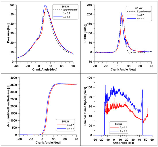
Figure 24.
Pressure, Rate of Heat Release, accumulated heat release and LFS in two cylinders.
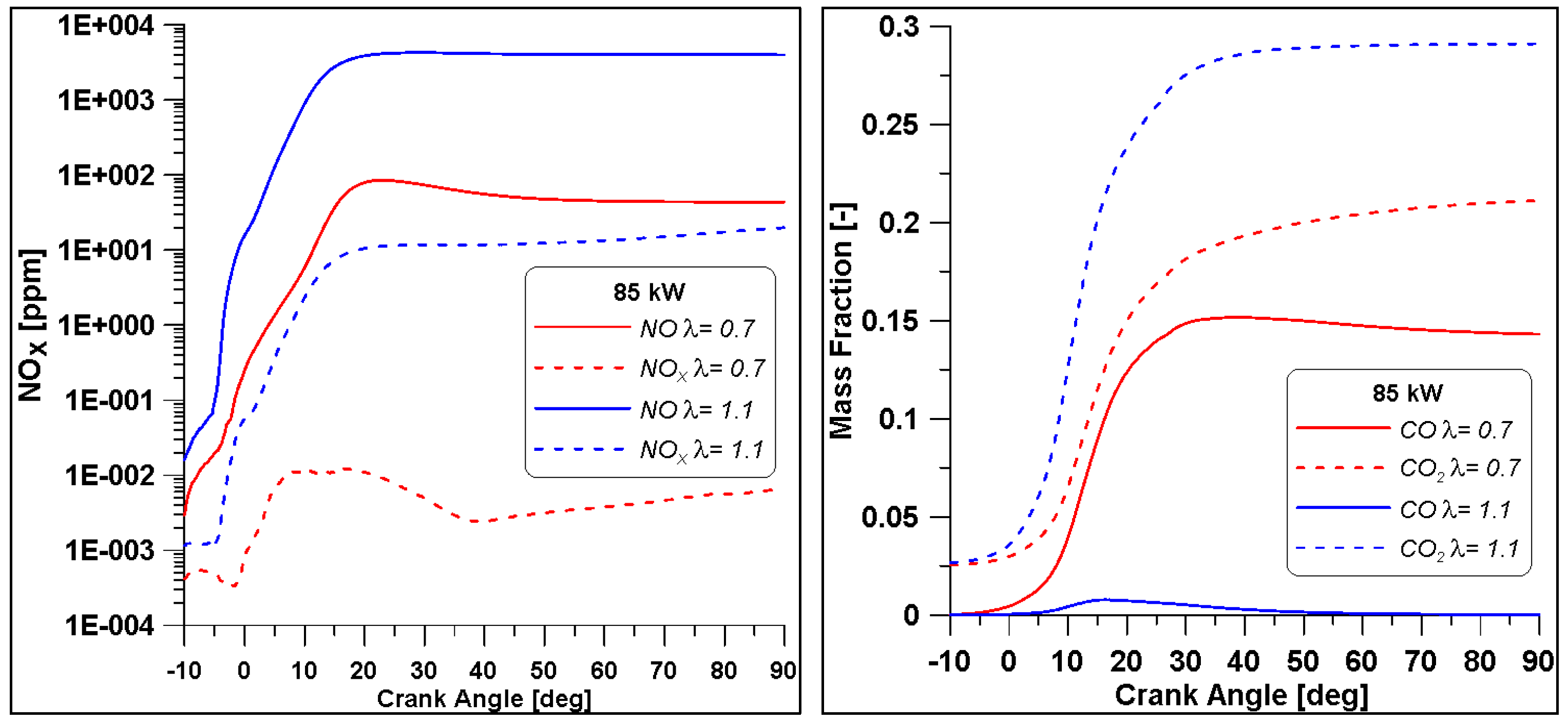
As said, another important aspect is represented by the pollutant emissions, reported in Figure 25. As expected, the cylinder which works with a higher λ foresees the formation of higher NOx; this is caused by the higher pressure and ROHR that imply an enhancement of temperature as well. Moreover, the higher concentration of oxygen favours the production of this pollutant. On the other hand, the same higher oxygen content in the mixture favours a significant reduction of CO production.
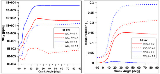
Figure 25.
Pollutant emissions for two cylinders. NUIG mechanism.
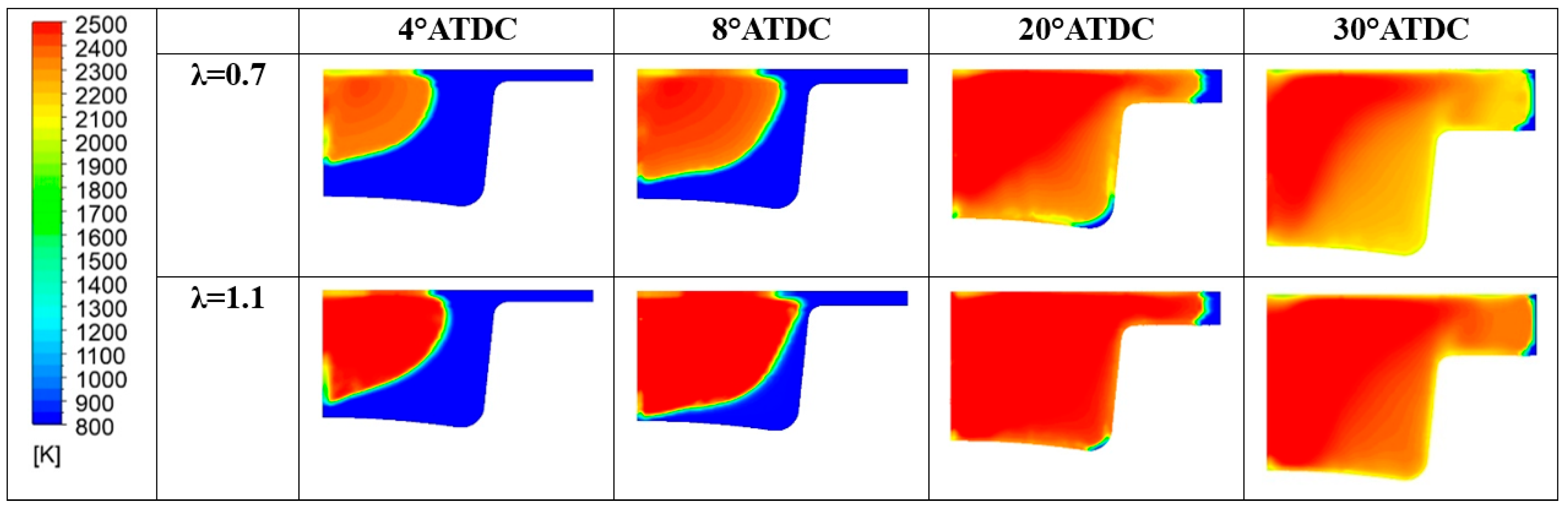
In Table 12, a summary of the main performance results for the two λ values is reported. Although the two cases feature a comparable level of gross IMEP, in the λ = 0.7 this is obtained at the expense of fuel consumption. Indeed, almost a double amount of fuel is introduced to achieve the same indicated work. Indeed, the λ = 0.7 demonstrates an inefficient conversion of the fuel represented by an unacceptable combustion and thermal efficiencies. As already evidenced the increase of the air-to-fuel ratio beyond slightly higher than the stoichiometric value leads to a beneficial drop of CO emission at the exhausts. Conversely, the high in-cylinder temperature (peak and extension of the region) illustrated in Figure 26 explains the increase of NOx emissions.
Table 12.
Results by varying λ value for the Low load.

Figure 26.
In-cylinder temperature distribution for different λ values.
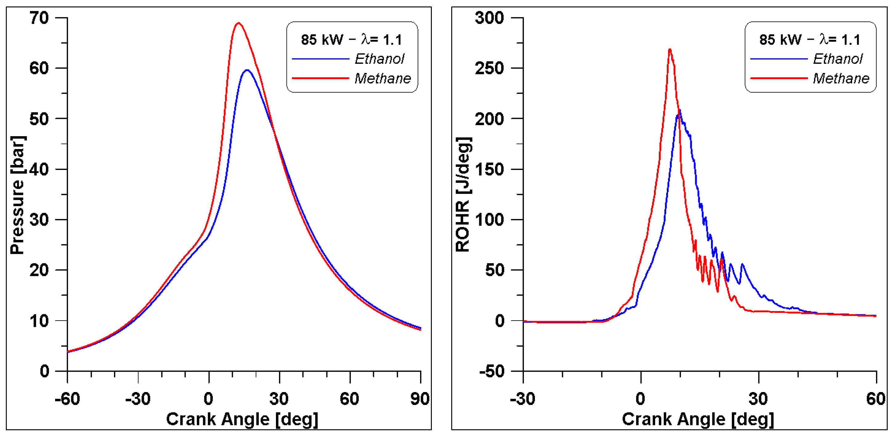
Finally, as mentioned in Section 1, the original engine was fuelled with natural gas (NG); therefore, a simulation is performed with NG which is considered pure methane, under the same operating conditions: λ equal to 1.1, and obtaining the same indicated work. From the comparison of the overall results in Table 13, it can be noted that there are no significant differences between the two fuels in terms of thermal efficiency. Pollutant emissions are on the same level, although methane produces slightly less CO and higher NOx. Nevertheless, as illustrated in Figure 27 by the in-cylinder pressure and the ROHR, the development of combustion features a different behaviour. The peak of pressure with methane is almost 10 bar higher with respect to ethanol, due to a faster ROHR, which can explain the slight increase in NOx in the exhaust gases.
Table 13.
Results by varying fuel at λ value fixed.
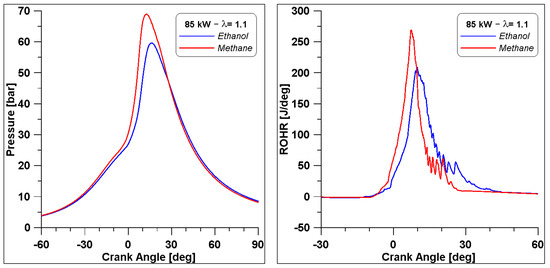
Figure 27.
Comparison of pressure and ROHR between ethanol and methane.
5.2. Medium-High Load Case (161 kW)
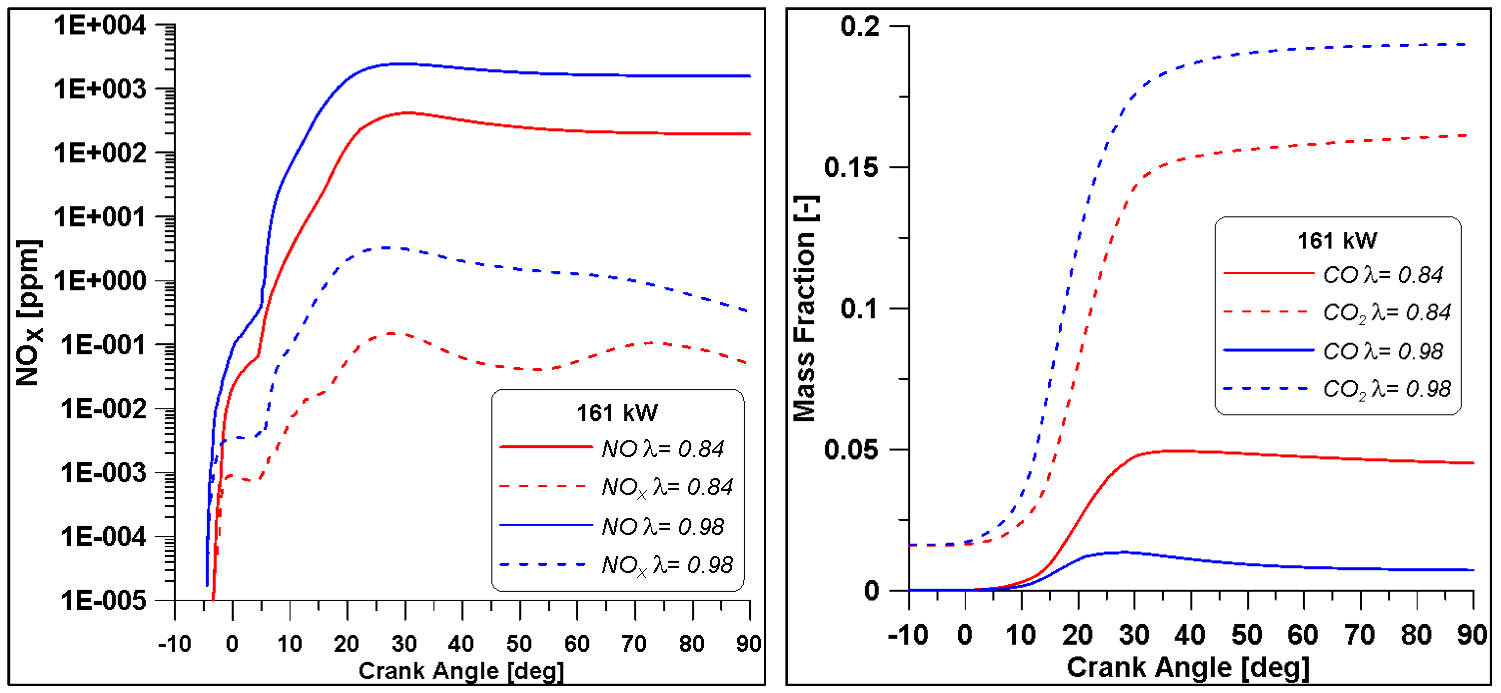
Similarly to the low load case, in the medium-high load case (161 kW), two cylinders with different λ values were examined. The cylinder #1 (equipped with the pressure transducer) features a λ = 0.84, while the best air-to-fuel ratio is found in cylinder #4 (λ = 0.98). In Table 14 a summary of the results is listed. With respect to the two cases analysed at low load level, these two λ values are closer, therefore fuel and energy inputs are comparable.
Table 14.
Results by varying λ value for the Medium-High load.
As previously observed, an air-to-fuel ratio closer to the stochiometric value allows for achieving better efficiency levels and again a trade-off between CO and NOx is observed. Nevertheless, in the reach case (λ = 0.84) the values of CO are halved with respect to low load case with λ = 0.7, while even in the λ = 0.98 lower NOx emissions are obtained.
The diagrams in Figure 28 demonstrate that the concentrations of NOx and CO are similar to those of the low load case but due to the increased load, the emission indices reported in Table 14 are reduced.
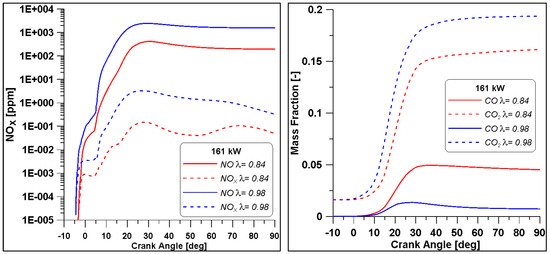
Figure 28.
Pollutant emissions by varying lambda for the Medium-High load.
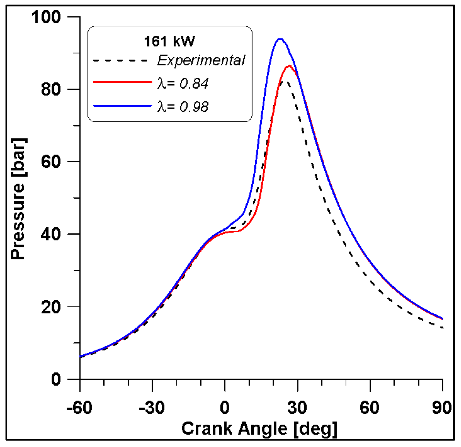
From Figure 29 it is observed that the in-cylinder pressure curve of the λ = 0.84 fairly reproduces the experimental trace until the peak, while an overestimation of the expansion phase occurs in the numerical simulations. By comparing the two λ values, if approaching the stoichiometric condition, the pressure levels increase by about 10 bar. In any case, from the ROHRs in Figure 30 the differences seem less evident. The numerical simulation describes a combustion duration almost equal to that obtained from the experimental measurements. In addition, this parameter shows that the increase of λ causes a reduction of the ignition delay that consequently leads to an increase of pressure.

Figure 29.
Pollutant emissions by varying lambda at Medium-High load.
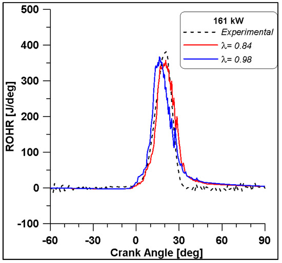
Figure 30.
ROHR by varying lambda at Medium-High load.
Finally, the LFS in Figure 31 highlight different values again, as anticipated by Figure 15; the λ = 0.98 features a faster speed that ceases slightly before the λ = 0.84 case (almost 3 degrees). In any case, all these differences are smaller with respect to the trends already observed in the low load case (Figure 24).
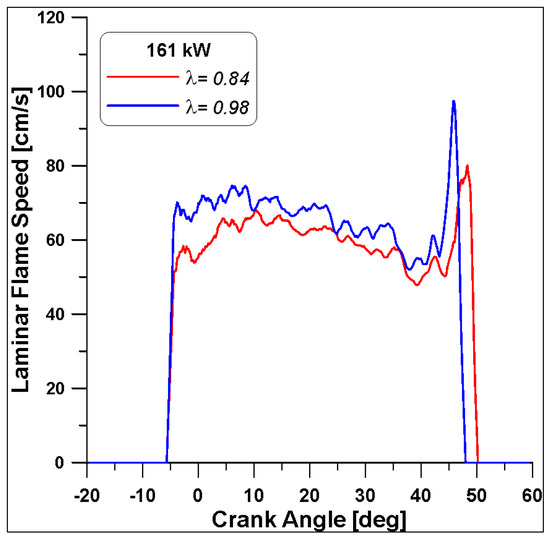
Figure 31.
Laminar flame speed by varying lambda at Medium-High load.
5.3. Sensitivity Analysis to Spark Timing—Low Load Case
With a view to optimizing the engine operation, in terms of reducing emissions, a sensitivity analysis of spark-ignition timing was carried out for the low load case for both λ values. In both cases, two advanced (25° and 30° BTDC) and one delayed (10° BTDC) SI timings are tested and compared with the value of 15° BTDC used in the experimental tests. In Table 15 and Table 16 a summary of the effect of spark timing is shown for the two λ values, while only for the λ = 0.7, trends of combustion parameters and emissions are illustrated in Figure 32 and Figure 33.
Table 15.
Results by varying spark timing, λ = 0.7.
Table 16.
Results by varying spark timing, λ = 1.1.
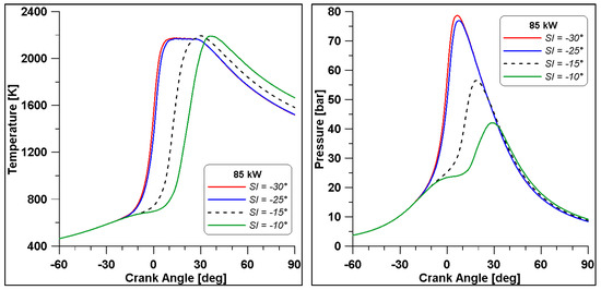
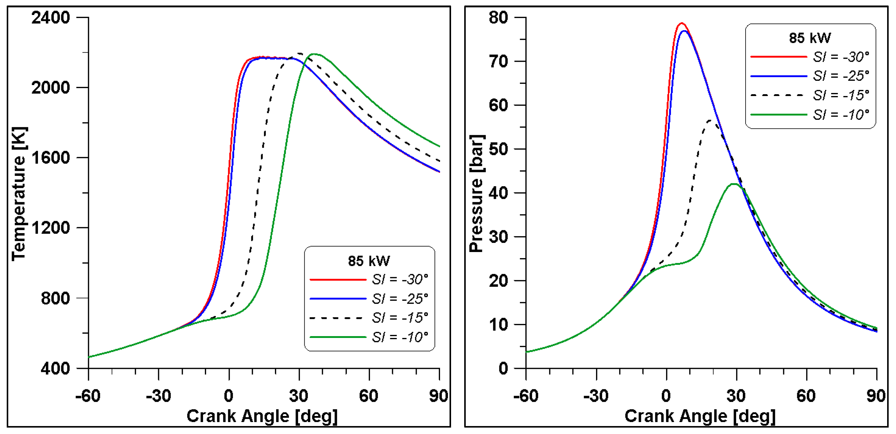
Figure 32.
In-cylinder temperature and pressure by varying the spark timing (λ = 0.7).
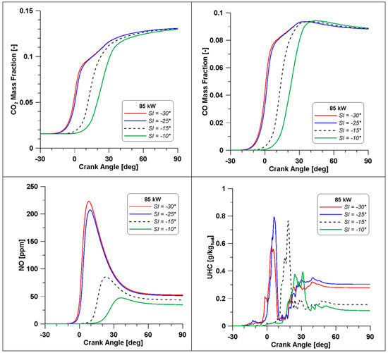
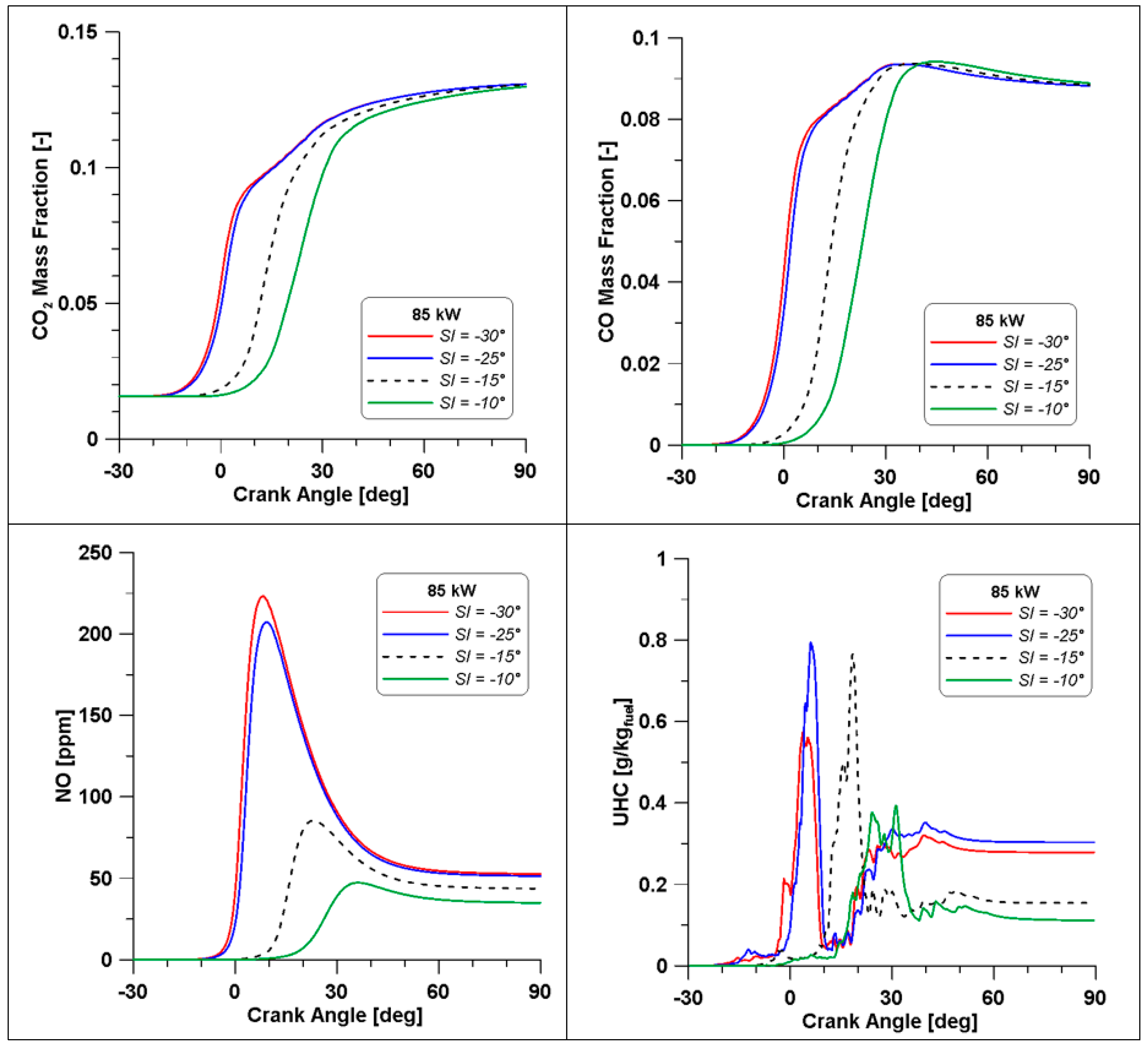
Figure 33.
Pollutant emissions by varying the spark timing (λ = 0.7).
The λ = 0.7 case is the most critical; the rich composition of the mixture does not allow significant improvements by changing the spark advance. From Table 15, it is clear that a delay of the spark event is only detrimental for performance while emissions are unaltered. Instead, a slight increase of gross IMEP and indicated work are observed for the anticipated cases. The most significant difference is represented by the maximum pressure, which rises to 20 bar. Emissions seem minimally affected by this strong enhancement of pressure. However, to better understand these results, it is necessary to analyse and discuss the in-cylinder curves displayed in Figure 32 and Figure 33.
In Figure 32 the in-cylinder mean temperature and pressure evidence that by advancing the SI, the maximum temperature and pressure are reached across the TDC. Temperature achieves a mean value of 2200 K, meaning that a great part of the domain is involved by this high temperature regime. This leads to a steep rise of pressure; however, there is no sign of knock occurrence.
As already mentioned, when referring to Table 15, emissions seem minimally affected by the strong enhancement of pressure, but the trends in Figure 33 demonstrate that high levels of temperature (and pressure) influence the formation of the most important species. Indeed, across the TDC, CO2 and CO displayed an evident change of slope; the higher temperatures cause a beneficial oxidation of CO but likely a dissociation of CO2 as well. Furthermore, a massive production of NO can be responsible for the drop in CO2, which is the natural product of combustion. In the end, at the exhaust, CO and CO2 emission converge for all cases to a similar value, as already observed in Table 15, while NO still features higher concentrations in the cases where temperature achieves the highest value.
Still, in the most advanced spark cases (30° and 25° BTDC), a significant residual fraction of unburned hydrocarbons is observed at the exhaust valve opening. The UHCs mainly consist of methane and other intermediate species whose formation is strictly related to ethanol decomposition. This phenomenon is temperature-dependent and, therefore, the wider crank angle interval that can be observed in the −30° and −25° cases (Figure 32) explains the enhanced formation of UHC. The same Figure 32 shows lower temperatures in the same cases during the expansion phase and this occurrence inhibits the final conversion of unburned species. The slightly lower values of combustion efficiency in Table 15 confirm these considerations.
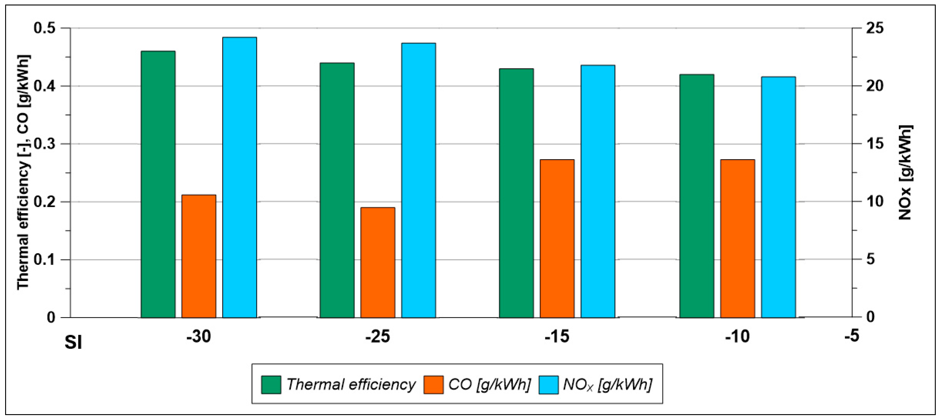
In the second case (λ = 1.1), a linear trend is observed for almost all parameters listed in Table 16. Again, although the greater amount of oxygen increases combustion and emissions formation rates with respect to λ = 0.7 case, a delayed spark advance presents the lowest engine performance, while the better results in terms of NOx emissions are the consequence of an unoptimized thermal cycle. The two advance cases lead to an enhancement of IMEPg and indicated work, an advanced barycentre of combustion, and a better exploitation of the fuel with more than acceptable thermal efficiency. Finally, since the scope of this section is the optimization of the engine performance, it is interesting to point out that the best results in terms of emissions are obtained for the spark ignition set at 25° BTDC.
6. Conclusions
In this work an ethanol-fuelled engine has been examined for two operating points (λ = 0.7 low and λ = 0.84 medium-high load) by using a commercial CFD code with an appropriate selection of sub-models and libraries for a thorough analysis of the main phenomena governing the in-cylinder process. The model has been validated via the available experimental data, which displayed rich air-to-fuel ratios and a non-uniformity fuel distribution among the six cylinders, consequent to the well-known difficulties of ethanol to vaporize. Such non-homogeneous configuration induced differences in both combustion developments and the pollutant emissions-based cylinder examined.
The model has been built after a proper sensitivity analysis of the computational mesh and of the most suitable chemical kinetic mechanism; in this regard, five kinetic mechanisms have been tested to find the best compromise in terms of accuracy and computational times.
For each load level, simulations have been performed for the two above-mentioned λ values because they were measured on the only cylinder equipped with a pressure transducer to prove the validity of the CFD model. Then, these cases were compared considering the best λ values measured on the other cylinders.
Finally, for the low load case only, a spark timing sensitivity analysis has been performed to define an optimal situation in terms of emissions and performance for the two mixture compositions (λ = 0.7 and 1.1).
Based on the results carried out, the main considerations are as follows:
- The WVU mechanism proved to be effective in the description of the combustion development; however, due to lacking a set of reactions specifically dedicated to the description of NOx formation, the NUIG mechanism is necessary.
- The calibration of the parameters of the flame speed demonstrated that the best value for the b1 factor is 2.85.
- For both loads, in the cylinder with a richer mixture, combustion occurs with delay and low thermal efficiency, the lower NOx values in the exhaust are given to the lower temperatures in the cylinder consequently to the inefficient combustion, unacceptable CO levels are also detected; on the contrary, where the mixture is lean or stoichiometric the greater presence of oxygen causes an enhancement of NOx and CO2 values but a beneficial reduction of CO.
- The operation of the cylinder with a low λ mixture is particularly critical especially at low load, resulting in incomplete combustion.
- To improve these results at low load, the spark timing is changed. However, when anticipating the ignition (SI = 25° BTDC and 30° BTDC) with respect to the reference value of 15° BTDC in the λ = 0.7, no significant improvements are obtained both in terms of performance and CO and NOx emissions. Instead, with a λ equal to 1.1 (see the histogram in Figure 34), the spark advance improves efficiency, the NOx index increases, while a minimum value of CO emissions is found for a SI of 25° BTDC.
 Figure 34. Pollutant emissions and combustion efficiency by varying spark timing (Low load; λ = 1.1).
Based on the outcomes from this analysis, authors’ work in the future will be carried out with more accurate fluid–dynamic simulations, including the open valve period for a more realistic prediction of the flow distribution inside the cylinders. This enhanced approach will also address different fuel injection strategies, in order to overcome the main drawbacks that have been evidenced in this paper.
Author Contributions
Conceptualization, M.C.C. and R.T.; methodology, M.C.C., R.D.R. and R.T.; software, R.D.R. and R.T.; validation, D.P. and T.C.; investigation, M.C.C., R.D.R. and R.T.; resources, M.C.C. and R.T.; data curation, R.D.R. and D.P.; writing—original draft preparation, R.D.R. and D.P.; writing—review and editing, M.C.C., R.D.R., R.T. and T.C.; visualization, R.D.R. and D.P.; supervision, M.C.C. and R.T.; project administration, T.C.; funding acquisition, M.C.C. and T.C. All authors have read and agreed to the published version of the manuscript.
Funding
This work was funded by the Next Generation EU—Italian NRRP, Mission 4, Component 2, Investment 1.1 “Fund for the National Research Program and Projects of Significant National Interest (PRIN)” (Directorial Decree n. 1409/2022) “PRIN 2022 PNRR” -Title of the Project: Bio-FIRed IC Engines for off-grid Electric Vehicles ChaRging Stations (Bio-FiRE-for-EVer), Project Code: P2022K9T2S, CUP E53D23017230001. This work reflects only the authors’ views and opinions, neither the Ministry for University and Research nor the European Commission can be considered responsible for them.
Data Availability Statement
The original contributions presented in this study are included in the article. Further inquiries can be directed to the corresponding author.
Acknowledgments
The CFD computations are licensed by ANSYS-Forte®. In memory of Professor Sergio Bova who encouraged and participated in this research.
Conflicts of Interest
The authors declare no conflicts of interest. The funders had no role in the design of the study; in the collection, analyses, or interpretation of data; in the writing of the manuscript; or in the decision to publish the results.
Abbreviations
| ATDC | After Top Dead Centre |
| BMEP | Brake Mean Effective Pressure |
| BSFC | Brake Specific Fuel Consumption |
| BTDC | Before Top Dead Centre |
| BTE | Brake Thermal Efficiency |
| CFD | Computational Fluid Dynamics |
| CI | Compression Ignition |
| COV | Coefficient of Variation |
| CR | Compression Ratio |
| DF | Dual Fuel |
| EGR | Exhaust Gas Recirculation |
| EV | Electric Vehicle |
| EVC | Exhaust Valve Close |
| EVO | Exhaust Valve Open |
| GHG | Greenhouse Gas |
| ICE | Internal Combustion Engine |
| IMEP | Indicated Mean Effective Pressure |
| ITE | Indicated Thermal Efficiency |
| IVC | Inlet Valve Close |
| IVO | Inlet Valve Open |
| LFS | Laminar Flame Speed |
| LHE | Latent Heat of Evaporation |
| LHV | Lower Heating Value |
| MAP | Manifold Air Pressure |
| NG | Natural Gas |
| PFI | Port Fuel Injected |
| RED | Renewable Energy Directive |
| RES | Renewable Energy Source |
| ROHR | Rate of Heat Release |
| SI | Spark Ignition |
| SPI | Single Point Injection |
| TDC | Top Dead Centre |
| TKE | Turbulent Kinetic Energy |
| UHC | Unburned Hydrocarbon |
| WOT | Wide Open Throttle |
References
- International Energy Agency Global Energy and Climate Model Documentation. Available online: www.iea.org (accessed on 5 May 2024).
- Henke, I.; Cartenì, A.; Beatrice, C.; Di Domenico, D.; Marzano, V.; Patella, S.M.; Picone, M.; Tocchi, D.; Cascetta, E. Fit for 2030? Possible Scenarios of Road Transport Demand, Energy Consumption and Greenhouse Gas Emissions for Italy. Transp. Policy 2024, 159, 67–82. [Google Scholar] [CrossRef]
- Electricity Generation in the European Union from 2020 to 2023, by Fuel. Available online: https://www.statista.com/statistics/800217/eu-power-production-by-fuel/ (accessed on 12 May 2024).
- Zou, Y.; Zhao, J.; Gao, X.; Chen, Y.; Tohidi, A. Experimental Results of Electric Vehicles Effects on Low Voltage Grids. J. Clean. Prod. 2020, 255, 120270. [Google Scholar] [CrossRef]
- Wang, Z.; Jochem, P.; Fichtner, W. A Scenario-Based Stochastic Optimization Model for Charging Scheduling of Electric Vehicles under Uncertainties of Vehicle Availability and Charging Demand. J. Clean. Prod. 2020, 254, 119886. [Google Scholar] [CrossRef]
- Fathabadi, H. Novel Standalone Hybrid Solar/Wind/Fuel Cell Power Generation System for Remote Areas. Sol. Energy 2017, 146, 30–43. [Google Scholar] [CrossRef]
- Domínguez-Navarro, J.A.; Dufo-López, R.; Yusta-Loyo, J.M.; Artal-Sevil, J.S.; Bernal-Agustín, J.L. Design of an Electric Vehicle Fast-Charging Station with Integration of Renewable Energy and Storage Systems. Int. J. Electr. Power Energy Syst. 2019, 105, 46–58. [Google Scholar] [CrossRef]
- Al Wahedi, A.; Bicer, Y. Assessment of a Stand-alone Hybrid Solar and Wind Energy-based Electric Vehicle Charging Station with Battery, Hydrogen, and Ammonia Energy Storages. Energy Storage 2019, 1, e84. [Google Scholar] [CrossRef]
- Al Wahedi, A.; Bicer, Y. Development of an Off-Grid Electrical Vehicle Charging Station Hybridized with Renewables Including Battery Cooling System and Multiple Energy Storage Units. Energy Rep. 2020, 6, 2006–2021. [Google Scholar] [CrossRef]
- Filote, C.; Felseghi, R.; Raboaca, M.S.; Aşchilean, I. Environmental Impact Assessment of Green Energy Systems for Power Supply of Electric Vehicle Charging Station. Int. J. Energy Res. 2020, 44, 10471–10494. [Google Scholar] [CrossRef]
- European Parliament and Council, Directive (EU) 2018/2001 of the European Parliament and of the Council on the Promotion of the Use of Energy from Renewable Sources. Available online: https://eur-lex.europa.eu/eli/dir/2018/2001/oj/eng (accessed on 11 June 2024).
- Li, Q.; Zhang, H. Spark-Ignited Kernel Dynamics in Fine Ethanol Sprays and Their Relations with Minimum Ignition Energy. Combust. Flame 2023, 249, 112622. [Google Scholar] [CrossRef]
- Örs, İ.; Yelbey, S.; Gülcan, H.E.; Sayın Kul, B.; Ciniviz, M. Evaluation of Detailed Combustion, Energy and Exergy Analysis on Ethanol-Gasoline and Methanol-Gasoline Blends of a Spark Ignition Engine. Fuel 2023, 354, 129340. [Google Scholar] [CrossRef]
- Salvi, B.L.; Subramanian, K.A.; Panwar, N.L. Alternative Fuels for Transportation Vehicles: A Technical Review. Renew. Sustain. Energy Rev. 2013, 25, 404–419. [Google Scholar] [CrossRef]
- Gainey, B.; Lawler, B. The Role of Alcohol Biofuels in Advanced Combustion: An Analysis. Fuel 2021, 283, 118915. [Google Scholar] [CrossRef]
- Zapata-Mina, J.; Restrepo, A.; Romero, C.; Quintero, H. Exergy Analysis of a Diesel Engine Converted to Spark Ignition Operating with Diesel, Ethanol, and Gasoline/Ethanol Blends. Sustain. Energy Technol. Assess. 2020, 42, 100803. [Google Scholar] [CrossRef]
- Li, X.; Li, D.; Liu, J.; Ajmal, T.; Aitouche, A.; Mobasheri, R.; Rybdylova, O.; Pei, Y.; Peng, Z. Exploring the Potential Benefits of Ethanol Direct Injection (EDI) Timing and Pressure on Particulate Emission Characteristics in a Dual-Fuel Spark Ignition (DFSI) Engine. J. Clean. Prod. 2022, 357, 131938. [Google Scholar] [CrossRef]
- Shetty, S.; Shrinivasa Rao, B.R. In-Cylinder Pressure Based Combustion Analysis of Cycle-by-Cycle Variations in a Dual Spark Plug SI Engine Using Ethanol-Gasoline Blends as a Fuel. Mater. Today Proc. 2022, 52, 780–786. [Google Scholar] [CrossRef]
- Blumreiter, J.; Johnson, B.; Zhou, A.; Magnotti, G.; Longman, D.; Som, S. Mixing-Limited Combustion of Alcohol Fuels in a Diesel Engine; SAE International: Warrendale, PA, USA, 2019. [Google Scholar]
- Stein, R.A.; Anderson, J.E.; Wallington, T.J. An Overview of the Effects of Ethanol-Gasoline Blends on SI Engine Performance, Fuel Efficiency, and Emissions. SAE Int. J. Engines 2013, 6, 470–487. [Google Scholar] [CrossRef]
- Wang, C.; Zeraati-Rezaei, S.; Xiang, L.; Xu, H. Ethanol Blends in Spark Ignition Engines: RON, Octane-Added Value, Cooling Effect, Compression Ratio, and Potential Engine Efficiency Gain. Appl. Energy 2017, 191, 603–619. [Google Scholar] [CrossRef]
- Thakur, A.K.; Kaviti, A.K.; Mehra, R.; Mer, K.K.S. Progress in Performance Analysis of Ethanol-Gasoline Blends on SI Engine. Renew. Sustain. Energy Rev. 2017, 69, 324–340. [Google Scholar] [CrossRef]
- Li, Y.; Gong, J.; Deng, Y.; Yuan, W.; Fu, J.; Zhang, B. Experimental Comparative Study on Combustion, Performance and Emissions Characteristics of Methanol, Ethanol and Butanol in a Spark Ignition Engine. Appl. Therm. Eng. 2017, 115, 53–63. [Google Scholar] [CrossRef]
- Almarzooq, Y.M.; Schoegl, I.; Petersen, E.L. Laminar Flame Speed Measurements of a Gasoline Surrogate and Its Mixtures with Ethanol at Elevated Pressure and Temperature. Fuel 2023, 343, 128003. [Google Scholar] [CrossRef]
- Catapano, F.; Di Iorio, S.; Magno, A.; Vaglieco, B.M. Effect of Fuel Quality on Combustion Evolution and Particle Emissions from PFI and GDI Engines Fueled with Gasoline, Ethanol and Blend, with Focus on 10–23 Nm Particles. Energy 2022, 239, 122198. [Google Scholar] [CrossRef]
- Elfasakhany, A. Investigations on the Effects of Ethanol–Methanol–Gasoline Blends in a Spark-Ignition Engine: Performance and Emissions Analysis. Eng. Sci. Technol. Int. J. 2015, 18, 713–719. [Google Scholar] [CrossRef]
- European Parliament and Council, Directive (EU) 2009/30/EC of the European Parliament and of the Council. Available online: https://eur-lex.europa.eu/LexUriServ/LexUriServ.do?uri=OJ:L:2009:140:0088:0113:EN:PDF (accessed on 12 June 2024).
- Bai, Y.; Luo, L.; van der Voet, E. Life Cycle Assessment of Switchgrass-Derived Ethanol as Transport Fuel. Int. J. Life Cycle Assess. 2010, 15, 468–477. [Google Scholar] [CrossRef]
- Doğan, B.; Erol, D.; Yaman, H.; Kodanli, E. The Effect of Ethanol-Gasoline Blends on Performance and Exhaust Emissions of a Spark Ignition Engine through Exergy Analysis. Appl. Therm. Eng. 2017, 120, 433–443. [Google Scholar] [CrossRef]
- Fan, Q.; Liu, S.; Qi, Y.; Cai, K.; Wang, Z. Investigation into Ethanol Effects on Combustion and Particle Number Emissions in a Spark-Ignition to Compression-Ignition (SICI) Engine. Energy 2021, 233, 121170. [Google Scholar] [CrossRef]
- Ran, Z.; Hariharan, D.; Lawler, B.; Mamalis, S. Exploring the Potential of Ethanol, CNG, and Syngas as Fuels for Lean Spark-Ignition Combustion—An Experimental Study. Energy 2020, 191, 116520. [Google Scholar] [CrossRef]
- Kolodziej, C.P.; Pamminger, M.; Sevik, J.; Wallner, T.; Wagnon, S.W.; Pitz, W.J. Effects of Fuel Laminar Flame Speed Compared to Engine Tumble Ratio, Ignition Energy, and Injection Strategy on Lean and EGR Dilute Spark Ignition Combustion. SAE Int. J. Fuels Lubr. 2017, 10, 2017-01-0671. [Google Scholar] [CrossRef]
- Suresh, D.; Porpatham, E. Influence of High Compression Ratio on the Performance of Ethanol-Gasoline Fuelled Lean Burn Spark Ignition Engine at Part Throttle Condition. Case Stud. Therm. Eng. 2024, 53, 103832. [Google Scholar] [CrossRef]
- Li, X.; Zhen, X.; Wang, Y.; Tian, Z. Numerical Comparative Study on Performance and Emissions Characteristics Fueled with Methanol, Ethanol and Methane in High Compression Spark Ignition Engine. Energy 2022, 254, 124374. [Google Scholar] [CrossRef]
- Liu, S.; Zhang, H.; Fan, Q.; Wang, W.; Qi, Y.; Wang, Z. Investigation of Combustion and Particle Number (PN) Emissions in a Spark Induced Compression Ignition (SICI) Engine for Ethanol-Gasoline Blends. Fuel 2022, 316, 123155. [Google Scholar] [CrossRef]
- Liu, S.; Lin, Z.; Zhang, H.; Fan, Q.; Lei, N.; Wang, Z. Experimental Study on Combustion and Emission Characteristics of Ethanol-Gasoline Blends in a High Compression Ratio SI Engine. Energy 2023, 274, 127398. [Google Scholar] [CrossRef]
- Mancaruso, E.; Sequino, L.; Vaglieco, B.M.; Cameretti, M.C.; De Robbio, R.; Tuccillo, R. CFD Analysis of the Combustion Process in Dual-Fuel Diesel Engine; SAE Technical Papers; SAE International: Warrendale, PA, USA, 2018. [Google Scholar]
- De Robbio, R.; Cameretti, M.C.; Mancaruso, E.; Tuccillo, R.; Vaglieco, B.M. CFD Analysis of Different Methane/Hydrogen Blends in a CI Engine Operating in Dual Fuel Mode; SAE Technical Papers; SAE International: Krakow, Poland, 2022. [Google Scholar]
- Roy, S.; Mishra, R.; Askari, O.; Jarrahbashi, D. Reduced Ethanol Skeleton Mechanism for Multi-Dimensional Engine Simulation. J. Energy Inst. 2023, 106, 101147. [Google Scholar] [CrossRef]
- University of Galway. Available online: https://www.universityofgalway.ie/combustionchemistrycentre/mechanismdownloads/ (accessed on 5 July 2024).
- Ranzi, E.; Frassoldati, A.; Stagni, A.; Pelucchi, M.; Cuoci, A.; Faravelli, T. Reduced Kinetic Schemes of Complex Reaction Systems: Fossil and Biomass-Derived Transportation Fuels. Int. J. Chem. Kinet. 2014, 46, 512–542. [Google Scholar] [CrossRef]
- Millán-Merino, A.; Fernández-Tarrazo, E.; Sánchez-Sanz, M.; Williams, F.A. A Multipurpose Reduced Mechanism for Ethanol Combustion. Combust. Flame 2018, 193, 112–122. [Google Scholar] [CrossRef]
- Wu, Y.; Panigrahy, S.; Sahu, A.B.; Bariki, C.; Beeckmann, J.; Liang, J.; Mohamed, A.A.E.; Dong, S.; Tang, C.; Pitsch, H.; et al. Understanding the Antagonistic Effect of Methanol as a Component in Surrogate Fuel Models: A Case Study of Methanol/n-Heptane Mixtures. Combust. Flame 2021, 226, 229–242. [Google Scholar] [CrossRef]
- Fagundez, J.L.S.; Sari, R.L.; Garcia, A.; Pereira, F.M.; Martins, M.E.S.; Salau, N.P.G. A Chemical Kinetics Based Investigation on Laminar Burning Velocity and Knock Occurrence in a Spark-Ignition Engine Fueled with Ethanol–Water Blends. Fuel 2020, 280, 118587. [Google Scholar] [CrossRef]
- De Robbio, R.; Cameretti, M.C.; Mancaruso, E.; Tuccillo, R.; Vaglieco, B.M. Combined CFD—Experimental Analysis of the In-Cylinder Combustion Phenomena in a Dual Fuel Optical Compression Ignition Engine; SAE Technical Papers; SAE International: Capri, Naples, Italy, 2021. [Google Scholar]
- Peters, N. Turbulent Combustion; Cambridge University Press: Cambridge, UK, 2000. [Google Scholar]
- ANSYS. Forte Theory Manual, Release 2024 R1; ANSYS: Canonsburg, PA, USA, 2024; Available online: http://www.ansys.com (accessed on 10 May 2024).


Disclaimer/Publisher’s Note: The statements, opinions and data contained in all publications are solely those of the individual author(s) and contributor(s) and not of MDPI and/or the editor(s). MDPI and/or the editor(s) disclaim responsibility for any injury to people or property resulting from any ideas, methods, instructions or products referred to in the content. |
© 2025 by the authors. Licensee MDPI, Basel, Switzerland. This article is an open access article distributed under the terms and conditions of the Creative Commons Attribution (CC BY) license (https://creativecommons.org/licenses/by/4.0/).