1. Introduction
The increasing demand for energy efficiency and sustainability in the building sector has led to substantial advances in smart building technologies. Smart Green Townhouses (SGTs) integrate Renewable Energy Sources (RESs), Internet of Things (IoT) devices, and advanced control systems to optimize energy consumption, reduce costs, and lower environmental impact. However, effective load management in residential buildings remains challenging due to the influence of occupant behavior on energy use patterns [
1,
2]. Occupant energy behavior is shaped by psychological and economic factors such as daily routines, comfort preferences, and decision-making habits [
3]. These factors are captured in the proposed framework by modeling occupancy patterns based on presence and usage tendencies. This enables real-time occupant-centric optimization for improved energy efficiency in dynamic residential environments.
Machine Learning (ML) has emerged as a powerful tool for managing the complexity of load forecasting and control in smart buildings [
4]. ML models allow for accurate prediction and effective control in real-time systems [
5,
6]. For example, hybrid deep learning architectures, such as the combination of Convolutional Neural Networks (CNNs) and Long Short-Term Memory (LSTM) networks, have been used for robust and accurate forecasting [
7]. CNN-LSTM models have been combined with metaheuristic algorithms like the Coati Optimization Algorithm for renewable energy forecasting [
8]. While these methods have proven effective, existing research does not sufficiently address the role of real-time occupant behavior in residential load optimization [
5,
6,
9].
Deep learning has been considered for equipment scheduling and energy control in dynamic systems [
10,
11]. However, few approaches provide real-time adaptability while balancing energy savings, cost efficiency, and occupant comfort. While occupancy-based HVAC prediction and control have been employed [
12,
13], integration with occupant-aware load forecasting has not been considered. Thus, a real-time, occupant-centric load optimization framework is proposed. This framework integrates a hybrid LSTM-CNN model with Multi-Objective Particle Swarm Optimization (MOPSO) to dynamically balance load demand, cost, emissions, and comfort. Public datasets and real-time IoT sensor data [
14,
15,
16] are used to enable intelligent control of systems such as HVAC and lighting based on actual occupancy and preferences. While LSTM-CNN models have been employed in energy forecasting, the integration with real-time occupant-centric data has not been considered. The results presented for Connected Smart Green Townhouses (CGSTs) demonstrate the applicability, scalability, and performance of the proposed framework in realistic residential scenarios.
The contributions of this work are as follows.
A hybrid LSTM-CNN model is proposed to predict load demand, cost, and emissions.
Occupant behavior is integrated into a dynamic multi-objective optimization framework.
The proposed framework is evaluated for four connected townhouses in Burnaby, British Columbia (BC), Canada. The results obtained indicate significant load reduction and cost savings while ensuring occupant satisfaction.
The remainder of this paper is structured as follows.
Section 2 presents the methodology and optimization algorithms. The performance is evaluated in
Section 3 and the results are discussed.
Section 4 provides some concluding remarks including the implications for residential load optimization.
2. Methodology
A hybrid LSTM-CNN model is employed for dynamic load, cost, and carbon emission prediction [
5,
6]. It was implemented using Python with Pandas for data manipulation, NumPy for calculations, and Matplotlib for visualization [
5]. Although the framework has been designed for real-time applications, model execution time and update frequency depend on available computational resources and sensor sampling rates. In the experiments, the hybrid LSTM-CNN model was used for prediction and optimization for a 24 h horizon within 12–18 s on a standard desktop computer which is sufficient for real-time hourly operation. The framework can be configured to run at hourly intervals for day-ahead optimization and at shorter intervals (e.g., 15 min) for finer control. An LSTM is used due to its ability to capture long-term dependencies and temporal patterns in sequential data, which is critical for accurate forecasting of loads influenced by occupant behavior and weather. A CNN is employed to extract local features and spatial correlations from multi-dimensional inputs such as occupancy and environmental data. In this paper, occupant behavior refers to measurable actions and patterns that affect residential energy consumption. This includes real-time presence detection (e.g., motion and door sensors), appliance usage habits (e.g., when and how long devices are used), HVAC and lighting preferences (e.g., thermostat setpoints, lighting usage), and feedback interactions with control systems. This behavior is inferred from IoT sensor data and smart devices to support dynamic load optimization.
The MOPSO algorithm is used to optimize the tradeoff between load efficiency, cost savings, and carbon emission reduction while ensuring occupant comfort. It was chosen considering the advantages and applicability to SGT systems [
5]. It is a well-established algorithm that has excellent convergence [
17], diversity preservation, and suitability for nonlinear, multi-objective problems. Here, MOPSO is used to effectively balance load, cost, and emissions while ensuring occupant comfort which is particularly challenging in real-time residential applications. This illustrates the practicality of MOPSO for the optimization of complex, dynamic building energy systems.
Real data from several sources is employed including occupancy and load demand data from [
14,
15], IoT sensor data from [
16], weather data from [
18,
19], and energy prices from [
18]. Data from IoT sensors (e.g., motion detectors, door sensors) and smart devices (e.g., thermostats) are integrated with utility data to infer occupancy patterns [
20]. The AMPds dataset [
14,
15] provides high-resolution time-series data on electricity, water, and natural gas consumption. This facilitates load demand modeling under seasonal and weather variations. IoT sensors support real-time adjustments due to changes in load [
16]. Energy-efficient technology such as heat pumps [
21] ensure efficient and sustainable SGTs [
22].
Although the focus here is on short-term, real-time occupant behavior, the proposed framework can easily be adapted to long-term patterns. Seasonal and holiday-related behavior can be captured using historical data to improve load prediction while maintaining adaptability to dynamic occupant profiles. However, the goal here is real-time prediction in a dynamic environment that is more challenging due to the very short time scale.
2.1. The Proposed Framework
The proposed framework uses publicly available datasets [
14,
15,
16] and real-time IoT data collected from SGTs [
5,
6]. To ensure consistency across diverse features, the data are normalized to the range [0, 1]. The normalization for load type
j (e.g., electricity, gas, water) and townhouse type
i is
where
is the load for townhouse type
i and load type
j at time
t,
is the maximum load for townhouse type
i and load type
j across the dataset, and
is the corresponding minimum load. This ensures that normalization is performed independently for each load and townhouse type to prevent any single parameter from dominating the total load profile due to differences in magnitude or units such as electricity (kWh), gas (m
3), and water (liters). The normalization for the
ith bedroom townhouse is
Normalization is critical for the performance of ML models so that features with a large numerical range do not disproportionately influence model learning. It also improves numerical stability and accelerates convergence, particularly for gradient-based optimizers such as ADAM used in the proposed LSTM-CNN model.
The electricity load in kilowatt-hours (kWh) is
where
,
, and
represent the demand from electrical appliances, lighting, and HVAC systems, respectively. The gas load is
where
is the volume of natural gas consumed and
is the calorific value of gas (kWh/m
3). The water load is
where
is the volume of water used and
is the energy required to pump, heat, and treat water (kWh/m
3).
The base (unoptimized) load demand at time
t is given by
where
is the total unoptimized load demand (kW) and
is the unoptimized renewable energy (e.g., PV power). The optimized load without occupant data at time
t is
where
is the optimized renewable energy (kW) and
is the battery energy used to offset grid demand (kW). The maximum limits for battery and grid power (
and
) are based on practical system design assumptions supported by real-world parameters.
is set in the range 5–10 kW. This aligns with commercially available residential-scale lithium-ion battery systems, and is consistent with industry-standard systems used in residential microgrids in Canada [
5,
6].
is set in the range 12–15 kW. This reflects typical urban service capacity in a townhouse unit in BC and aligns with empirical values used in predicting load management for smart grid applications [
9,
13]. These values are not dictated by specific regulations but are based on realistic operating conditions and previous research.
The optimized load with occupant data at time
t considers occupant-driven factors and is given by
where
accounts for real-time occupancy-based load optimization including HVAC demand adjustments considering presence, load shifting to avoid peak times, and adaptive appliance control (e.g., delayed washing machine cycles). Substituting (
7) in (
8) gives
2.2. LSTM-CNN Model
The LSTM is used to capture temporal patterns in the input data to learn dependencies over time. The hidden state at time
t is
where
is the input at time
t which includes features such as load demand and occupancy data,
and
are weight matrices for the input data and previous hidden state, respectively,
is the bias term, and
is the sigmoid activation function
This function limits values to the range
and helps the network learn complex, non-linear relationships by introducing smooth gradients and preventing large outputs.
The CNN extracts spatial features from multi-dimensional data. The CNN output is
where
x is the input data structured as a two-dimensional (2D) matrix,
is 2D convolution given by
where
W is the convolutional filter (kernel) used to extract local patterns, and
is the bias term. The kernel is a small matrix of learnable weights used to extract spatial features from the input data. During training, it slides across the input matrix to learn local patterns such as occupancy and appliance usage. This helps improve the prediction capability of the model. The bias terms are randomly initialized and updated each iteration via backpropagation using the ADAM optimizer.
The combined LSTM and CNN output is
where
is the fusion function which here is concatenation. The average training time was 4.6 h. A dropout rate of 0.2 is applied after each LSTM and CNN layer to prevent overfitting. The model was trained using the Adam optimizer with a learning rate of 0.001 and batch size of 64.
The MOPSO algorithm objective function is
where
is the total load demand in kWh that includes all electrical appliances, HVAC systems, and other energy-consuming devices within the building
is the operational costs
is the carbon emissions,
N is the number of time steps,
is the electricity cost per kWh,
is the carbon emission factor in kg CO
2/kWh, and
, and
are weights representing the importance of each objective. The weights used here are
,
, and
. They were selected empirically to balance the three goals: load efficiency, operational cost reduction, and carbon emission reduction and are the result of extensive evaluation across many scenarios. Parameter tuning was conducted to ensure that no single objective disproportionately dominates the optimization. The corresponding constraints are
where
is the load supplied by the grid (kWh),
is the load met by renewable sources (kWh), and
is the energy supplied from battery storage (kWh).
To maintain occupant comfort, the deviation between the actual and desired indoor temperature should be within an acceptable range
where
is the actual indoor temperature at time
t,
is the corresponding desired temperature, and Threshold is the maximum acceptable cumulative deviation over the
N time steps (optimization period). This ensures energy savings do not compromise thermal comfort so load scheduling decisions account for occupant preferences.
2.3. Performance Metrics
Occupant comfort satisfaction is based on thermal comfort, lighting adequacy, and feedback adherence. The thermal comfort measures how close the indoor temperature is to the desired temperature and is given by
where 5 °C is considered the maximum difference. The lighting adequacy assesses how well lighting levels meet occupant needs. It is based on the percentage of time that the lighting intensity stays within the desired range and is expressed as
where
is the actual lighting intensity in room
i at time
t,
and
are the minimum and maximum acceptable light levels,
is an indicator function that returns 1 if the lighting is within the desired range, and 0 otherwise, and
r is the number of rooms. Feedback adherence measures how well the building systems (e.g., HVAC, lighting) respond to occupant feedback and is given by
where
is the number of feedback requests that were implemented by the system at time
t and
is the corresponding number of feedback requests submitted by occupants.
The occupant comfort satisfaction at time
t is a weighted sum of thermal comfort, lighting adequacy, and feedback adherence and is expressed as
where
,
, and
. These weights are based on the relative importance of thermal comfort, lighting adequacy, and feedback adherence in the overall comfort of the occupants.
The performance evaluation metrics are
where
n is the number of data values,
is the
ith predicted value from the ML model,
is the corresponding actual value, and
is the mean of the actual values given by
The MAE is the average magnitude of the prediction errors so smaller values indicate better accuracy. The RMSE measures the standard deviation of prediction errors, penalizing larger errors more heavily than the MAE. Lower values indicate higher accuracy. indicates how well the model explains the variations in the actual data. Values closer to 1 signify better model performance.
3. Performance Results
The results presented in this section were generated using OpenStudio (v3.4.0) for load simulation with and without occupant input. Data analysis and optimization were performed using Python v3.11.5 with Pandas v2.1.1 and Matplotlib v3.8.0 [
5,
6]. Real-time occupancy data was collected with ThingSpeak v2.0 [
23].
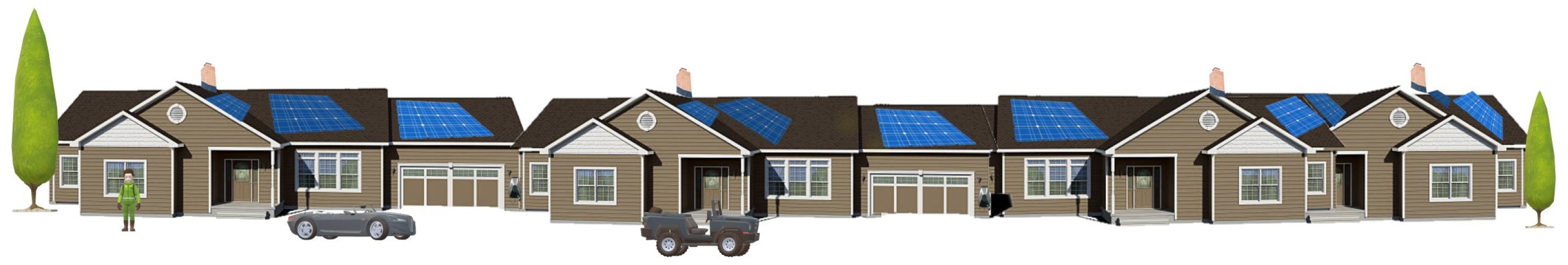
We consider a CSGT complex with 1-bedroom, 2-bedroom, 3-bedroom, and 4-bedroom units as shown in
Figure 1. Connected townhouses include two key components: connected water systems [
14,
24] and party walls [
25,
26]. Party walls are shared walls between adjacent properties and are jointly owned and maintained by property owners. Party wall agreements outline the responsibilities for maintenance, repairs, alterations, and dispute resolution.
Table 1 gives the SGT parameters including the number of residents, occupancy, hot water usage, lighting, EV charging, HVAC consumption, shared wall insulation, and fire safety.
Table 2 presents the base and optimization results with and without occupant data for the CSGT complex. The percentage reduction compared to the base results is also given. This indicates a significant improvement in load efficiency, cost savings, and carbon emission reduction. The load is decreased by 10.6% without occupant data and 14.3% with occupant data, confirming the effectiveness of real-time adaptive load management. Operational costs are reduced by up to 13.0% and carbon emissions are 11.0% and 15.5% lower, respectively. Peak load is reduced by 10.5% and 14.0% which helps grid stability and lowers peak-hour costs. Overall, occupant-centric optimization increases load efficiency, cost savings, and environmental performance, making CSGTs a practical solution for the future.
While the proposed framework benefits significantly from real-time occupant data, there are practical challenges in data acquisition. These include sensor inaccuracies, intermittent connectivity, and privacy concerns related to monitoring occupant presence and preferences. In this study, these issues were mitigated by using anonymized data collection protocols, leveraging non-intrusive IoT sensors (e.g., motion detectors, smart thermostats), and implementing local edge-processing to minimize data transmission risks.
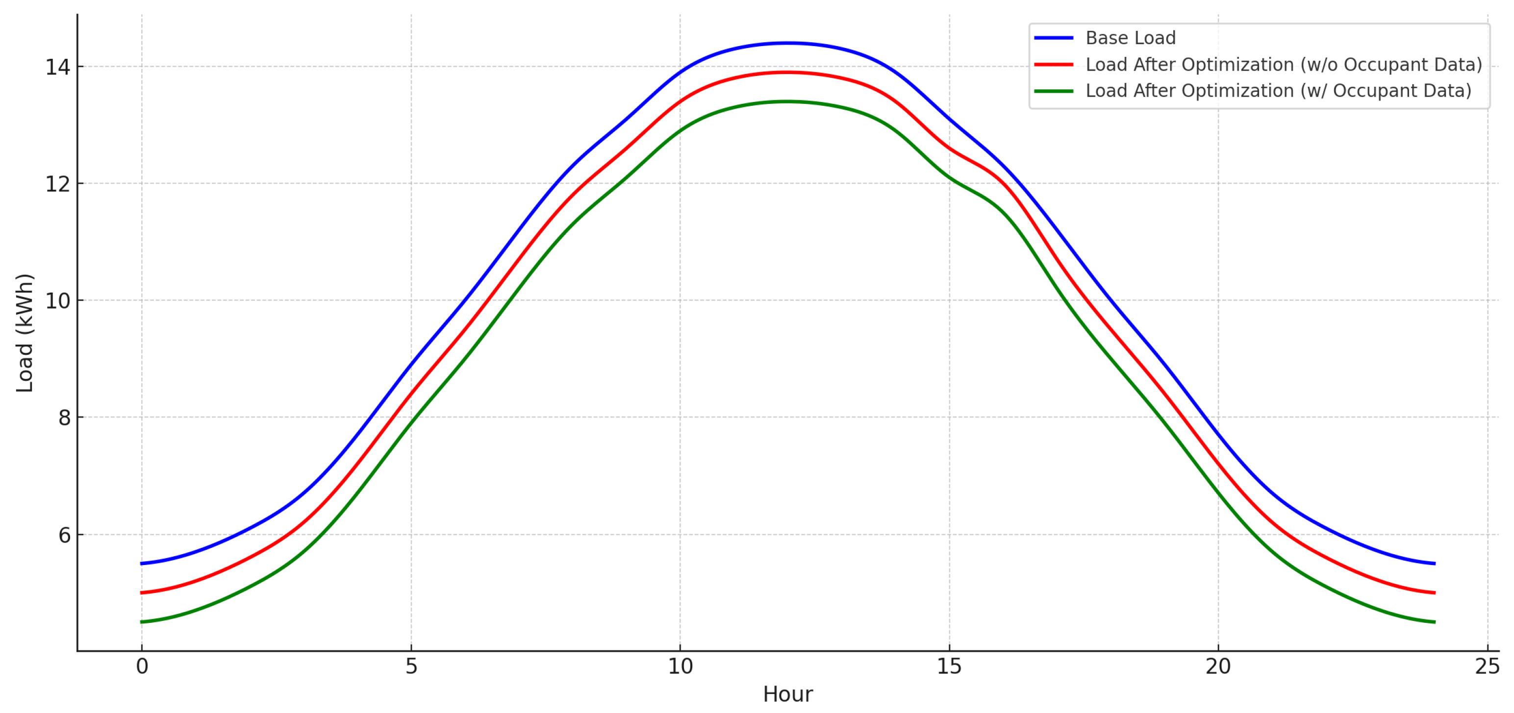
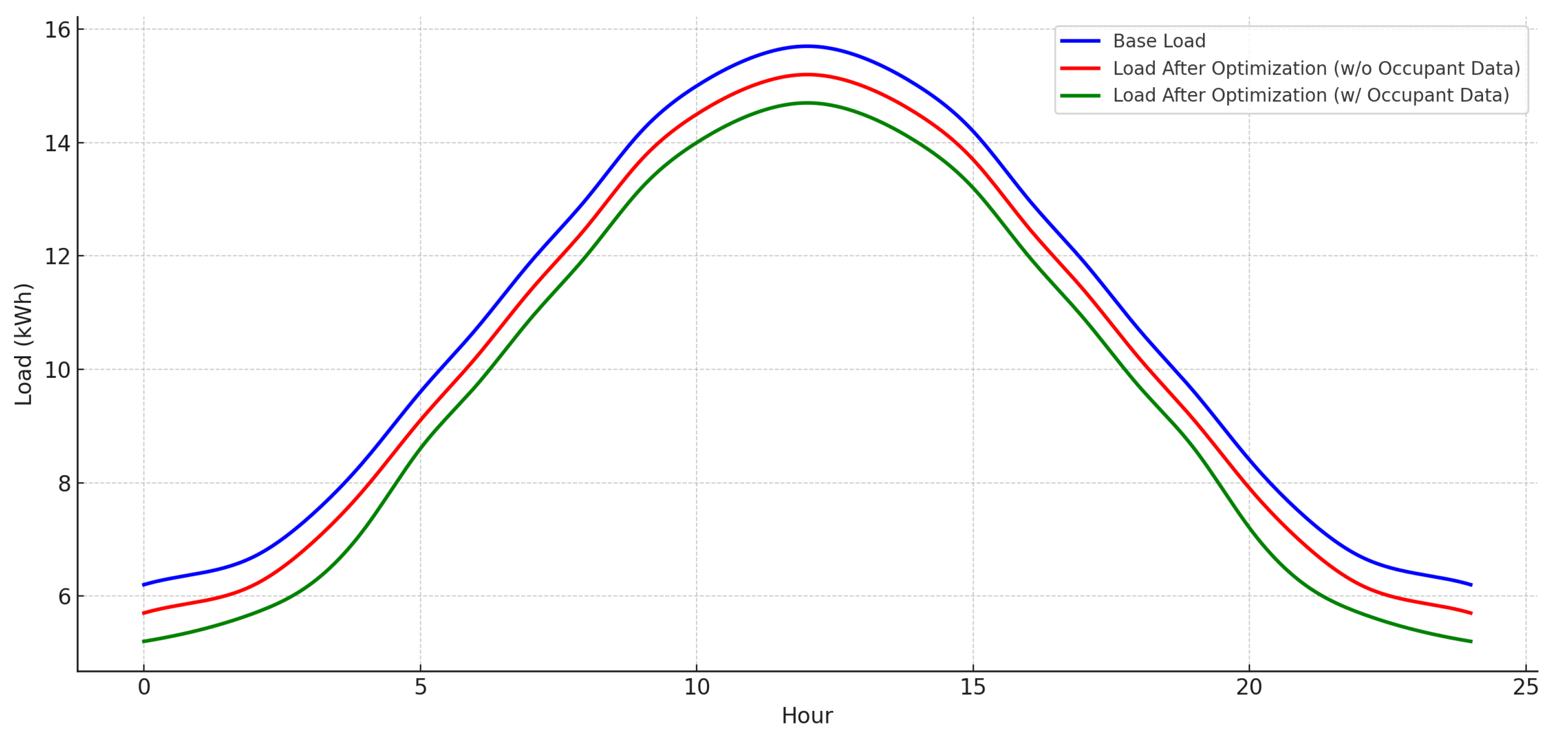
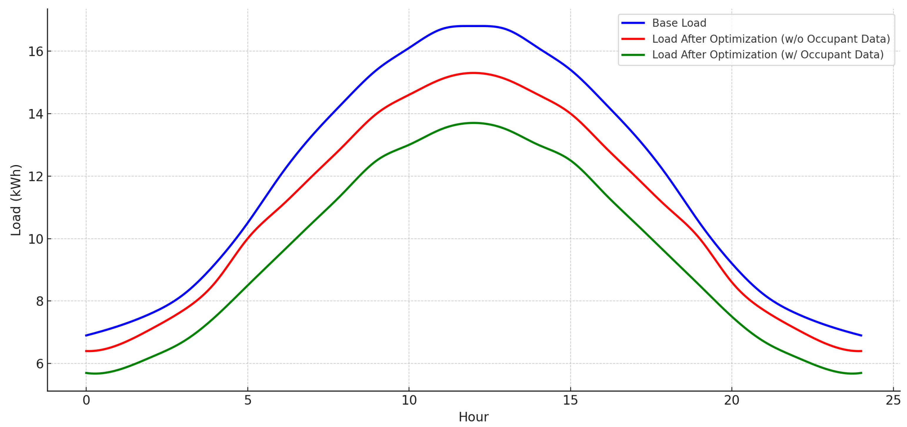
Figure 2,
Figure 3,
Figure 4 and
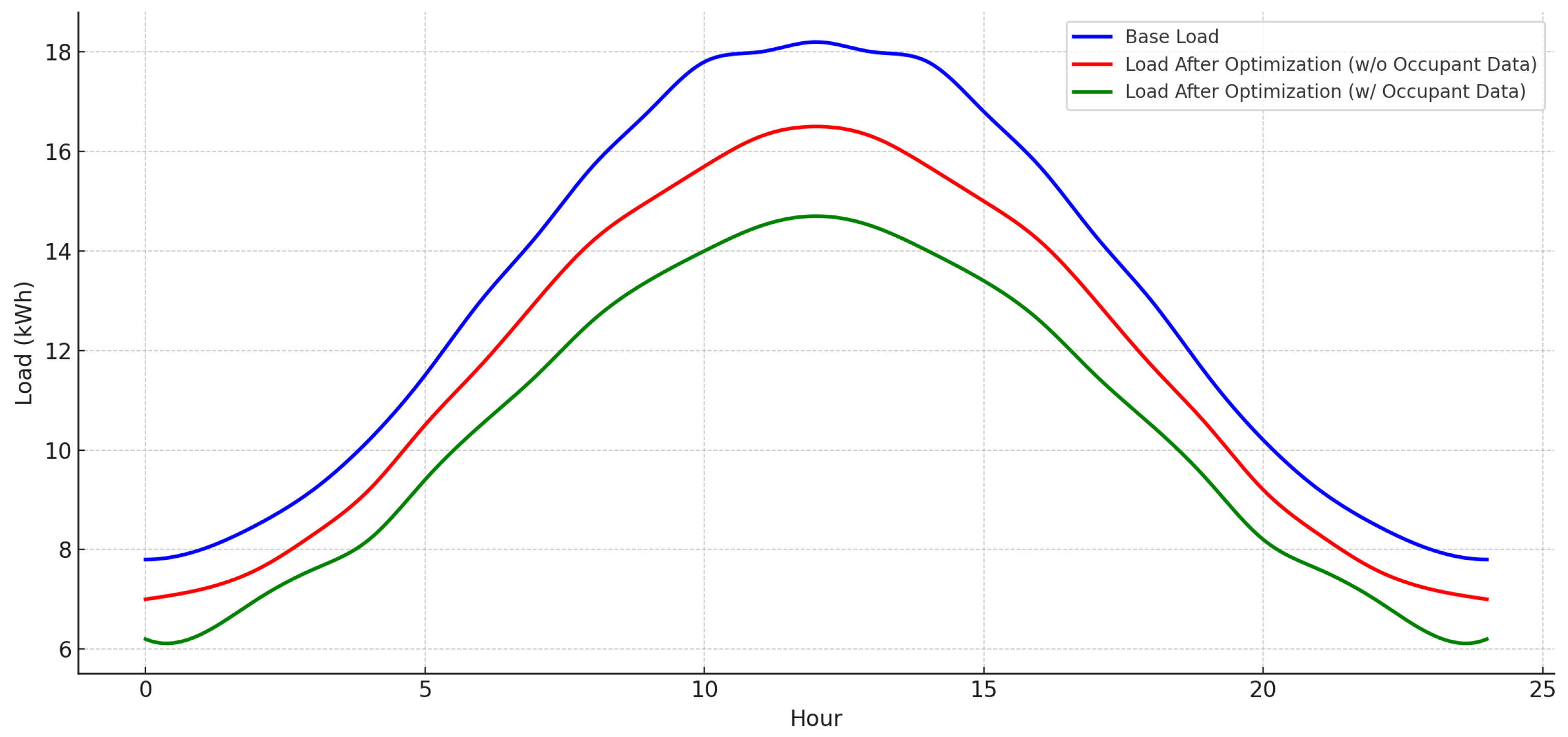
Figure 5 present the base load, optimized load without occupant data, and optimized load with occupant data for the individual CSGTs over a 24 h period.
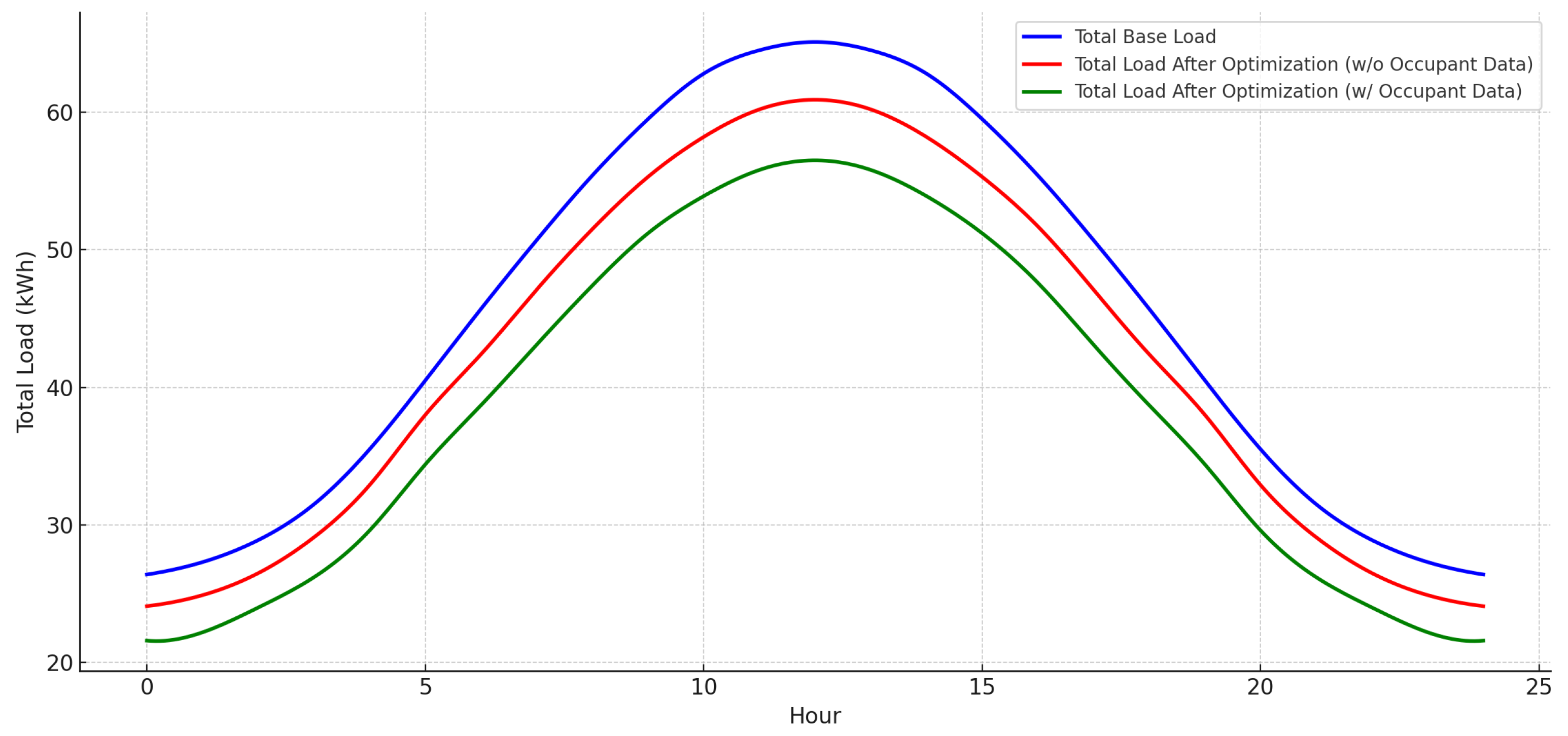
Figure 6 gives the corresponding results for the CSGT complex. Occupant data includes real-time and historical information on occupant presence, behavior, and preferences collected via sensors, IoT devices, smart meters, and user inputs [
5,
6,
14]. These results indicate that occupant-aware optimization improves load efficiency and reduces peak demand. For example, the 1-bedroom CSGT has a base load peak of 14.3 kWh, and this decreases to 13.9 kWh without occupant data and 13.3 kWh with occupant data. The 2-bedroom unit has a peak load reduction from 15.7 kWh to 15.2 kWh and 14.7 kWh. The 3-bedroom and 4-bedroom CSGTs have base peak loads of 16.8 kWh and 18.1 kWh, respectively, and they decrease to 15.3 kWh and 16.4 kWh without occupant data and 13.8 kWh and 14.5 kWh when occupant data is incorporated.
Figure 6 indicates that the cumulative effect is a significant decrease in the complex peak load from nearly 67 kWh to 61 kWh without occupancy data and 54 kWh with this data. These results demonstrate the value of real-time occupancy data in dynamic energy management, enabling control strategies that adapt load profiles to actual usage patterns and occupancy conditions. They also confirm that the proposed framework effectively improves load efficiency and lowers operational costs and carbon emissions while ensuring occupant comfort.
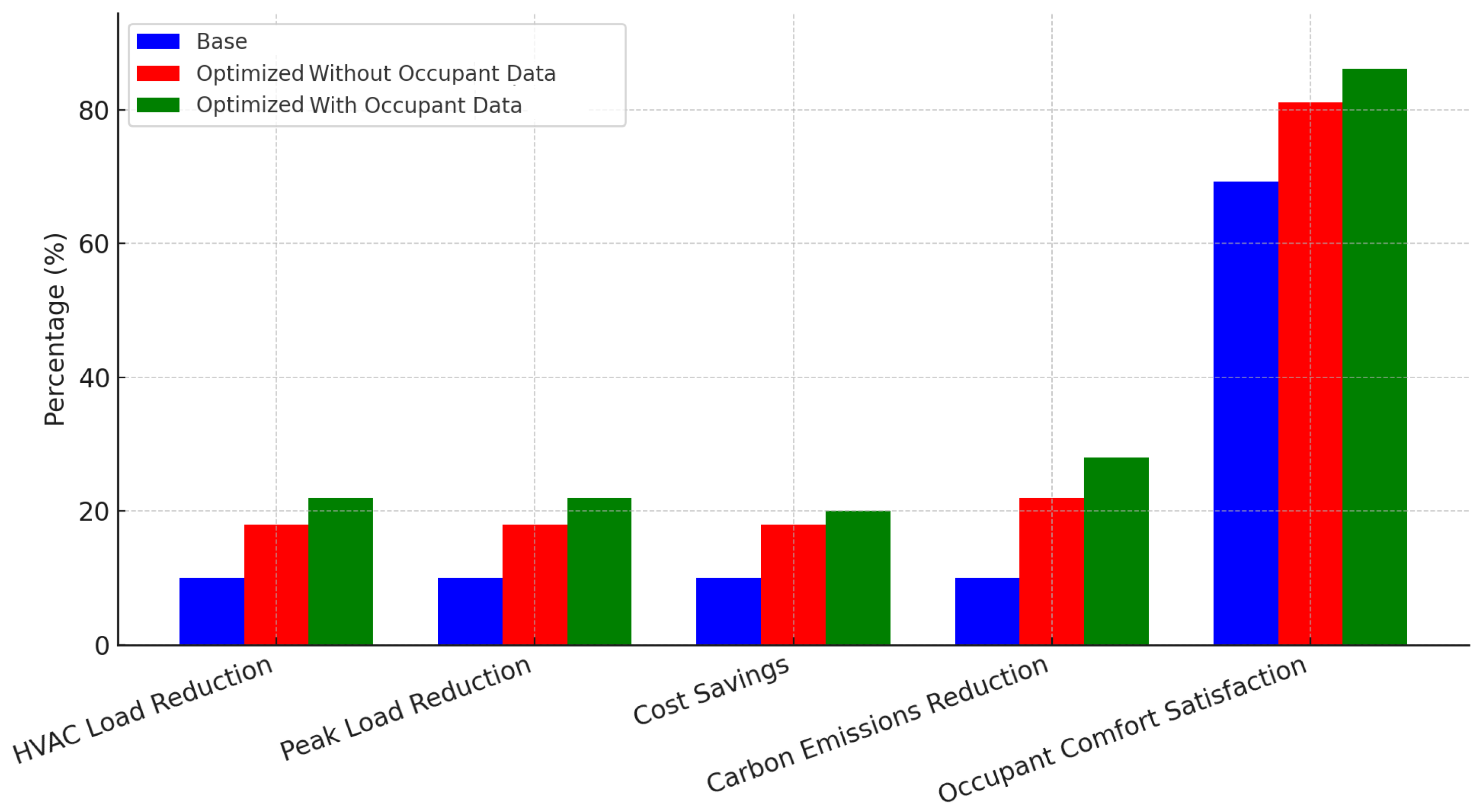
Figure 7 presents the townhouse complex base, optimized without occupant data, and optimized with occupant data HVAC and peak load reductions, cost savings, carbon emissions reduction, and occupant comfort satisfaction compared to the historical data in [
14,
15,
16]. The base results are the worst as optimization improves all five parameters. For example, optimization without occupant data provides an improvement in HVAC and peak loads of about 18%, and with occupant data there is an additional 2–6% improvement for all parameters. In particular, occupant comfort satisfaction is improved to over 85%. These results show the effectiveness of incorporating real-time occupant data into load management to improve efficiency, reduce costs, and lower environmental impact while maintaining a high level of occupant satisfaction.
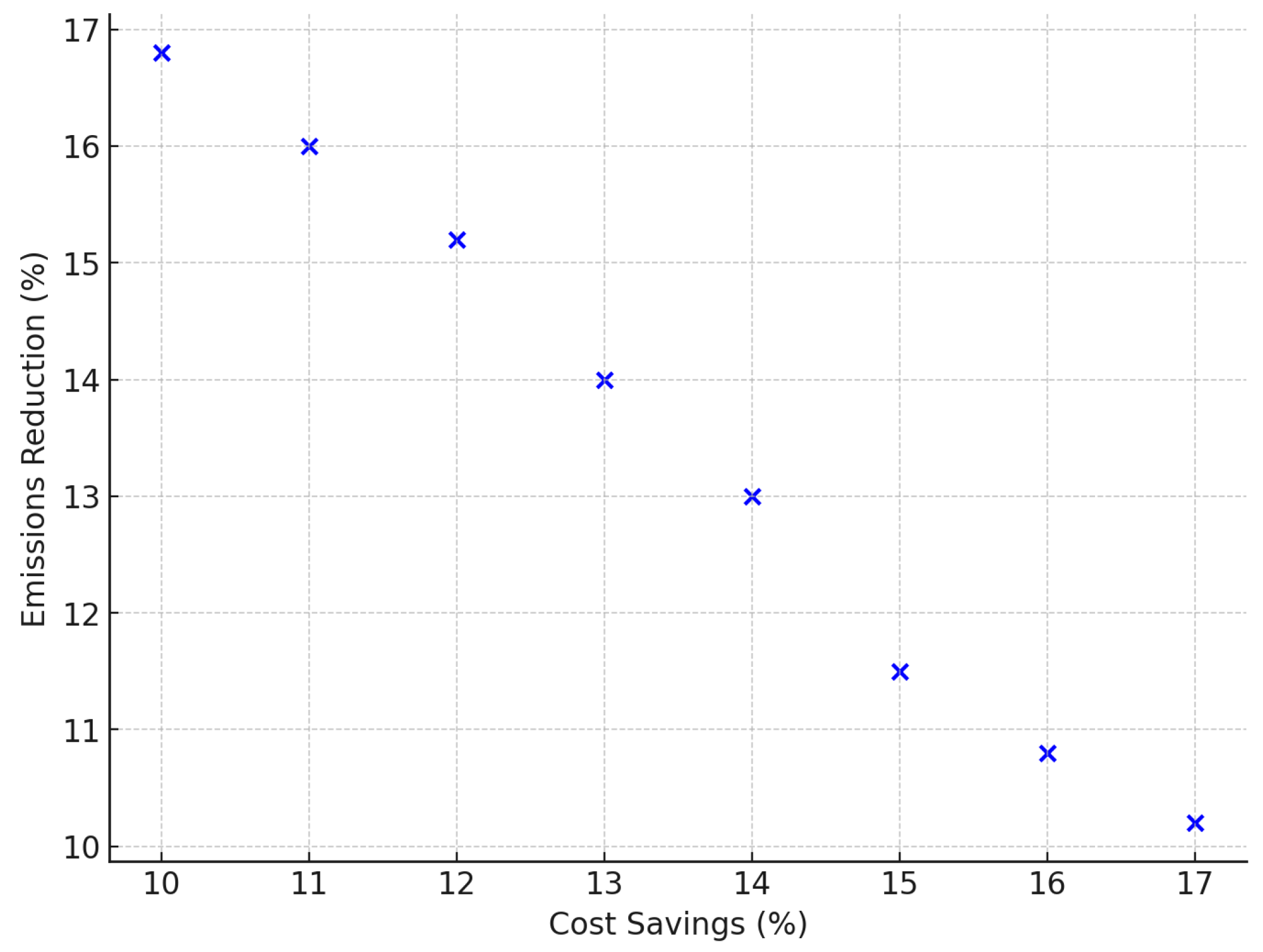
Figure 8 gives the cost savings versus emissions reduction for the townhouse complex optimized with occupant data. This shows the tradeoff between economic and environmental benefits with cost savings between 10% and 17%, and emission reductions between 10% and 17%. This reflects optimization considering load demand and occupant behavior and indicates an inverse relationship between the two parameters. Thus, reducing the environmental impact increases costs.
Figure 9 presents the townhouse complex occupant satisfaction in terms of thermal comfort, lighting adequacy, and feedback adherence for the base, optimized without occupant data, and optimized with occupant data cases. These results indicate optimization increases all three parameters. For example, thermal comfort increased from a base of approximately 67% to 80% optimized without occupant data and 86% optimized with occupant data. The corresponding lighting adequacy improved from 75% to 83% and 89%, and the feedback adherence from 60% to 72% and 82%. This confirms the effectiveness of occupant-aware energy optimization in improving occupant satisfaction.
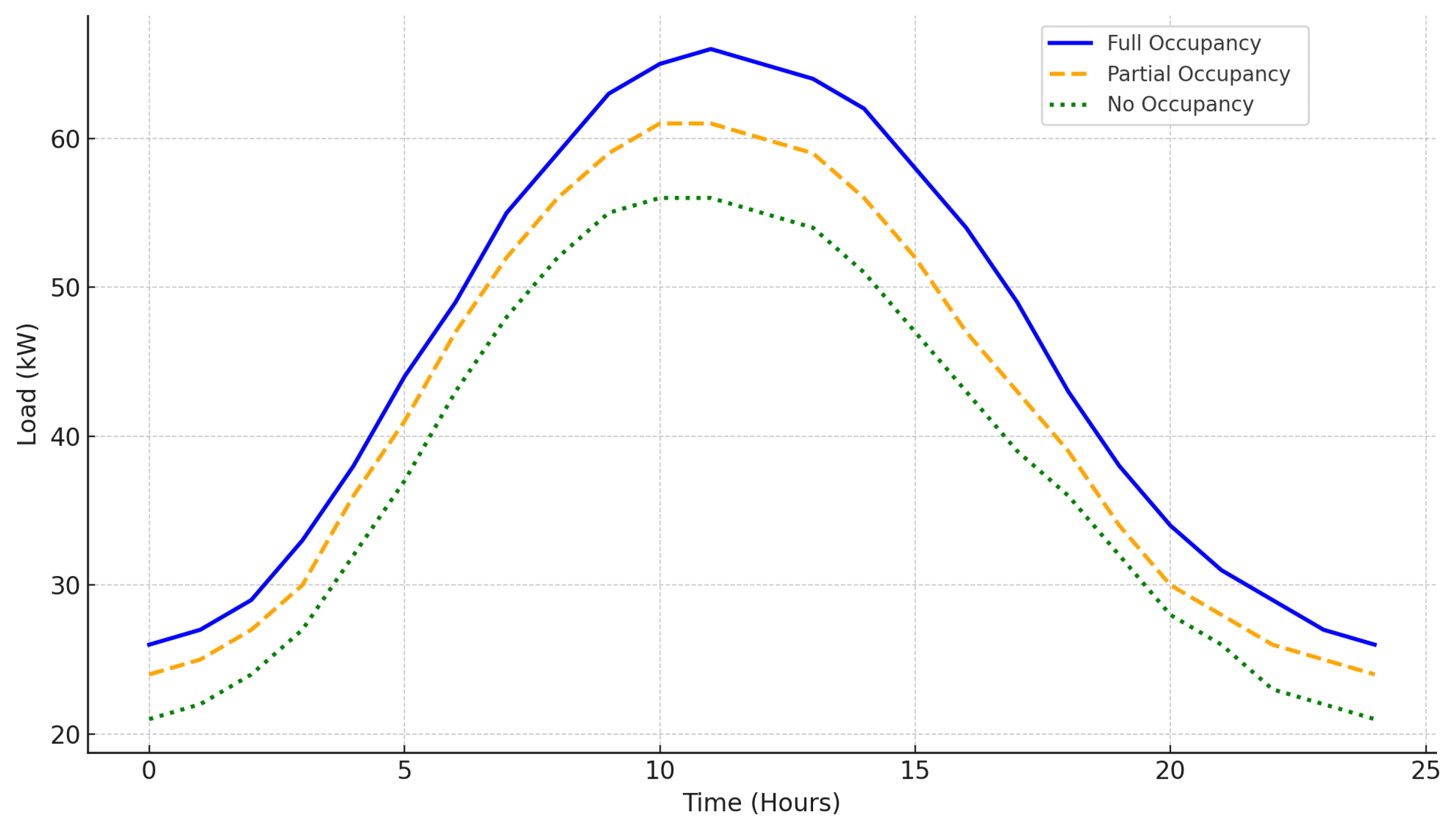
Figure 10 illustrates the impact of occupancy on the CSGT complex optimized load with occupant data over a 24 h period. Full occupancy indicates all residents are present which results in significant HVAC, lighting, and appliance use. With partial occupancy, there are fewer residents so energy consumption is lower. No occupancy means the building is unoccupied so only essential systems are running such as standby appliances, HVAC with setback control, and water heating. The results in
Figure 10 show that occupancy has a significant effect on load demand. With full occupancy, the peak load is about 66 kW at midday due to increased appliance and HVAC usage. Partial occupancy has a lower peak load of about 61 kW, reflecting moderate demand due to fewer residents. No occupancy has the lowest peak load which is below 57 kW. Thus, occupancy-driven load optimization is important to reduce peak demand and overall CSGT load. The performance improvements observed, i.e., reductions in load, operational cost, and carbon emissions, are a result of the integration of the prediction capability of the hybrid LSTM-CNN model and the dynamic capability of the MOPSO algorithm. The LSTM effectively captures time-dependent occupancy and load trends, while the CNN identifies spatial usage patterns from sensor inputs across multiple zones and townhouses. This reduces grid dependence during peak hours and aligns energy use with occupant presence, which lowers energy demand, utility costs, and greenhouse gas emissions.
Table 3 presents the MAE, RMSE, and
for the CSGT complex load optimization with the Linear Regression (LR), LSTM, CNN, and proposed hybrid LSTM-CNN models. The LR model has the worst performance with an MAE of 0.80 kWh and RMSE of 1.20 kWh, indicating poor prediction accuracy. The LSTM model has an MAE of 0.60 kWh and an RMSE of 0.72 kWh, which is lower. The CNN model improves on these results with an MAE of 0.56 kWh and an RMSE of 0.75 kWh. Further,
is 0.93 which is better than with the LR and LSTM models. The proposed model provides the best overall performance with the lowest MAE (0.47 kWh) and RMSE (0.68 kWh), and the highest
(0.95), indicating superior prediction accuracy and reliability. These results validate the effectiveness of the model in energy load forecasting. While the proposed model outperforms the others, its decisions are less interpretable due to the deep learning architecture. Incorporating explainable AI techniques can improve understanding of the input-output relationships, particularly for stakeholders seeking clarity in operational decisions.
Sensitivity of Key Parameters
The impact of key parameters is now considered.
Occupant Behavior Weights (, , ): Increasing the weight assigned to thermal comfort (e.g.,
from 0.4 to 0.6) will improve temperature satisfaction but also increase HVAC usage, potentially raising energy consumption by up to 8% [
12]. Similarly, a higher feedback adherence weight (
) will improve personalization but may introduce variations that will reduce energy efficiency.
Optimization Objective Function Weights (, , ): Adjusting the MOPSO weights shifts the balance between load, cost, and emissions. Prioritizing emissions (
) will reduce carbon emissions but increase reliance on storage and renewable energy, resulting in higher costs [
18,
19]. On the other hand, emphasizing cost (
) will improve affordability but may lower occupant satisfaction due to less flexible HVAC control.
MOPSO Parameters: As observed in [
17], larger swarm sizes or increased cognitive/social weights improve convergence but require longer computation times which may not be feasible for real-time applications.
Model Hyperparameters (e.g., depth, learning rate): Deep architectures such as LSTM and CNN can provide better accuracy but risk overfitting, especially with small datasets [
7,
8]. A properly tuned architecture balances prediction accuracy and generalizability. The hyperparameters used here are based on the results in [
5,
6].


 ,
, 

