Abstract
To address the charging demand challenges brought about by the widespread adoption of electric vehicles, integrated photovoltaic–storage–charging stations (PSCSs) enhance energy utilization efficiency and economic viability by combining photovoltaic (PV) power generation with an energy storage system (ESS). This paper proposes a two-stage data-driven holistic optimization model for the siting and capacity allocation of charging stations. In the first stage, the location and number of charging piles are determined by analyzing the spatiotemporal distribution characteristics of charging demand using ST-DBSCAN and K-means clustering methods. In the second stage, charging load results from the first stage, photovoltaic generation forecast, and electricity price are jointly considered to minimize the operator’s total cost determined by the capacity of PV and ESS, which is solved by the genetic algorithm. To validate the model, we leverage large-scale GPS trajectory data from electric taxis in Shenzhen as a data-driven source of spatiotemporal charging demand. The research results indicate that the spatiotemporal distribution characteristics of different charging demands determine whether a charging station can become a PSCS and the optimal capacity of PV and battery within the station, rather than a fixed configuration. Stations with high demand volatility can achieve a balance between economic benefits and user satisfaction by appropriately lowering the peak instantaneous satisfaction rate (set between 70 and 80%).
1. Introduction
Environmental pollution has become one of the most serious threats to human health in urban life. The transportation sector, as one of the primary contributors to pollution, exerts a particularly severe negative impact on the environment [1]. Therefore, reducing greenhouse gas emissions such as carbon dioxide from this sector has become an urgent and critical task. Among the various solutions, the promotion of electric vehicles (EVs) is regarded as one of the most feasible and effective measures [2]. With their advantages of zero emission, low noise, and high energy efficiency, EVs not only contribute to substantial reductions in environmental pollution but also play a crucial role in advancing carbon peaking and achieving the goals of carbon neutrality.
Currently, China, the world’s largest EV market, has seen a surge in EV ownership, rising from 2.11 million in 2018 to 18.13 million by June 2024 [3]. While this rapid growth significantly contributes to reducing environmental pollution, it also brings new challenges—most notably, the increasing regional and temporal concentration of charging demand. As EV users are primarily concentrated in urban areas and tend to charge their vehicles at night or during peak electricity consumption periods, this centralized charging behavior results in sharp spikes in grid load. This phenomenon may lead to localized power shortages and drive up electricity costs. Moreover, the uneven distribution of charging infrastructure exacerbates the problem, with some areas facing a shortage of charging stations, while others experience low utilization rates.
In order to mitigate the impact of EV charging on the distribution grid, initiatives to connect EV charging stations (EVCSs) to local renewable energy sources have been proposed and implemented in some regions [4]. For instance, Karmaker et al. [5] integrated solar photovoltaic (PV) panels and biogas generators into EVCS in Bangladesh, taking into account local resource availability. Among various renewable sources, solar PV is particularly favored due to its wide availability and the ease of installation on flat rooftops. Mouli et al. [6] explored the feasibility of integrating solar PV with workplace-based EVCS in the Netherlands and analyzed the corresponding PV system design. Zhang et al. [7] proposed a distributed PV-based EVCS layout. PV is not only readily available but can also be effectively integrated with charging stations to improve efficiency on both the grid side and the user side. On the grid side, Hung et al. [8] examined the efficiency of PV generation and the potential of grid-interactive PV systems to reduce energy loss and peak demand. They also developed a set of formulas for determining the optimal size of workplace PV charging stations. On the user side, Satya et al. [9] designed and modeled a plug-and-play solar PV power plant capable of charging an EV up to 80% within 10.25 min.
However, the PV industry faces the challenge of a high solar curtailment rate due to mismatches between generation and consumption. To address this issue, it is essential to incorporate an energy storage system (ESS) into PV charging stations, which can store excess solar energy during peak generation periods and release it during peak demand [10]. By combining PV stations with ESSs, integrated photovoltaic–storage–charging stations (PSCSs) can effectively utilize solar resources to supply clean energy for EVs during daylight hours, while ensuring a stable power supply at night or during peak demand periods through stored energy. Such stations not only enhanced solar energy utilization [11] but also mitigated the stochastic and intermittent nature of PV generation [12]. Therefore, this study conducts an in-depth investigation into the optimal siting and capacity configuration of PSCS.
In conducting siting and capacity optimization research for PSCS, it is essential to first accurately and reliably characterize EV charging demand. The existing studies primarily adopt two types of approaches to achieve this: simulation-based and data-driven methods. The simulation-based approach relies on prior assumptions about user behavior to construct probabilistic models. For example, Yang et al. [13] assumed that charging behaviors follow Gaussian distributions; Gómez [14] assumed that EV arrival times at charging stations follow a normal distribution. Wang et al. [15] further developed probabilistic models based on multiple behavioral dimensions, such as charging start time and duration. Once the distribution curves are defined, system simulation or Monte Carlo methods are used to simulate large-scale virtual vehicle charging demand under various travel scenarios, producing statistically stable load forecasts. For instance, Kim et al. [16] employed Monte Carlo simulation to evaluate the steady-state reliability of wind-powered EV charging stations by constructing a joint probabilistic model of EV load and wind power output under uncertainty. Dai et al. [17] applied the Erlang-B queuing model to simulate EV arrivals in their capacity optimization of PSCS, analyzing the trade-off between service quality and system capacity. Although this category of methods is straightforward and well-suited for preliminary planning, it often lacks fidelity to real-world user behavior due to its reliance on hypothetical assumptions, limiting its ability to capture the complexity of actual charging patterns. In contrast, data-driven approaches mine real-world charging behaviors by analyzing historical data such as GPS trajectories, charging records, and parking duration and location. For example, Kong et al. [18] integrated points of interest and vehicle dwelling data using an improved DBSCAN algorithm to identify optimal station locations. Li et al. [19] combined geographical constraints and energy efficiency metrics within a K-means clustering framework to detect high-demand charging zones. Zhang et al. [20] constructed a temporal distribution model of taxi movements based on representative time-period location data, revealing temporal variation in charging demand. Junker et al. [21] analyzed PV and battery storage configuration strategies based on operational data. While data-driven approaches offer greater realism, most of the above studies focus on either the temporal dimension [20,21] or the spatial dimension [19,20] in isolation, without systematically modeling the joint spatiotemporal effects that influence EV charging behavior.
In fact, spatiotemporal heterogeneity in EV charging demand is prevalent in urban environments. Charging behavior varies significantly across functional areas—for instance, residential zones typically experience peak demand during non-working hours (18:00 to 08:00), while commercial zones concentrate demand during working hours (08:00 to 17:00) [22]. Ignoring such differences can lead to unbalanced load distributions—some stations may be overloaded while others remain underutilized—thereby reducing both operational efficiency and economic viability of the integrated system. Therefore, considering only temporal or spatial factors in isolation is insufficient to support high-quality siting and configuration decisions.
After determining the EV charging demand, PSCSs are primarily optimized through siting [23,24], charge/discharge scheduling [25,26], or capacity planning [27,28] to achieve grid-side management objectives—such as reducing peak–valley load differences [23,24,25,26] and improving the utilization efficiency of renewable energy sources [27,28]. For instance, Deeum et al. [23] proposed an optimization model for siting charging stations integrated with PV and ESS in active distribution networks, focusing on grid stability and operational efficiency. Liu et al. [25] developed a controlled EV charging strategy considering demand-side response and local wind/PV resources, guiding users to charge during off-peak hours via time-of-use pricing. Sun et al. [27] proposed a multi-objective design framework for fast-charging stations integrating PV and ESS, targeting minimal operational cost and pollutant emissions.
These studies contribute significantly to enhancing grid resilience, reducing peak loads, and promoting energy conservation. However, they still face two major limitations:
First, there is a lack of economic assessment and commercial feasibility analysis from the operator’s perspective. The high investment cost and long payback period of PV and ESS necessitate the careful consideration of factors such as equipment utilization, economic return, and dynamic electricity pricing. Without this, such systems risk high capital expenditure with limited financial return, hindering large-scale deployment under market-oriented mechanisms. As direct investors in charging infrastructure, operators’ profitability directly influences their willingness to adopt PV-ESS solutions.
Second, many studies treat siting and capacity planning as separate problems, ignoring the influence of siting on demand characteristics, which further affects optimal configuration strategies. In reality, siting determines the potential user base and significantly shapes the demand pattern, which, in turn, affects the feasibility and economic rationale of integrating PV or ESS. For example, a site serving mainly daytime demand with high electricity prices is ideal for PV deployment; in contrast, stations with nighttime demand may require larger storage systems, raising construction costs. Therefore, siting decisions and load profiles directly inform supply scheme requirements. Reference [28] is one of the few studies that considers the impact of demand pattern variations across different areas on the capacity optimization of PSCS. However, it assumes fixed demand patterns for the same type of functional areas across different regions without accounting for the influence of siting decision variables.
To address these challenges, jointly optimizing siting and capacity planning while uncovering the spatiotemporal patterns of charging demand is essential to enhancing the operational efficiency of PSCSs. Thus, this paper proposes a two-stage integrated optimization model: the first stage determines station sitings and charging piles configurations based on responsive charging demand; the second stage optimizes the capacities of PV panels and ESSs in accordance with on-site demand distribution to minimize the operator’s total cost. The main contributions of this study are as follows:
- Driven by large-scale EV trajectory data, this study reveals the spatiotemporal heterogeneity of charging demand and its impact on the configuration of PSCS, thereby enhancing the accuracy of demand-driven planning.
- From an operator perspective prioritizing operational cost, we propose a capacity optimization model for PSCS. The existing studies often overlook the compatibility of PV panels and ESSs with specific charging sites—a gap this study addresses through a tailored framework. Furthermore, by ensuring operator profitability, the proposed approach supports charging network expansion and accelerates EV adoption.
- From a system-wide perspective, this study synergistically optimizes the site selection and capacity configuration of PSCS. This integrated strategy overcomes limitations in the existing studies—separating site selection and capacity planning (“siting-on-siting” or “capacity-on-capacity”).
The remainder of this paper is organized as follows: Section 2 introduces the system architecture of the PSCS. Section 3 details the solution approach for the two-stage optimization model, covering siting and capacity configuration. Section 4 presents a real-world case study in Shenzhen to demonstrate the applicability of the model, while the sensitivity analysis of key parameters is detailed in Section 5. Finally, the conclusion summarizes the main findings and outlines future research directions.
2. Data-Driven Two-Stage Siting and Capacity Optimization Model
To achieve the comprehensive optimization of PSCS, this study proposes a data-driven two-stage optimization framework that sequentially tackles the siting and capacity planning problems. At a high level, the first stage focuses on identifying optimal siting for charging stations based on observed EV travel behavior, while the second stage determines the most cost-effective ESS configuration for each selected site, considering the temporal dynamics of charging demand.
In the first stage, the goal is to uncover where charging stations should be sited to best serve actual demand patterns. Thus, spatiotemporal trajectory data of EVs are analyzed to detect regions of high travel density, which serve as proxies for charging needs. The spatiotemporal density-based spatial clustering of applications with noise (ST-DBSCAN) algorithm is employed to identify these high-frequency travel areas. Once clusters are formed, their centroids are extracted using the K-means algorithm to define candidate station sitings. For each site, the number of potential charging demands is aggregated on an hourly basis, creating a temporal demand profile. The peak-hour demand is then used to estimate the minimum number of charging piles required to ensure acceptable service quality during high-load periods.
In the second stage, the identified demand patterns are translated into station-specific dynamic load curves, which serve as input for a coordinated capacity planning model. This model jointly optimizes the configuration of PV panels and ESSs at each site, aiming to minimize the total cost of the energy supply infrastructure. The result is a cost-efficient allocation of PV modules and battery units tailored to the load characteristics of each charging station.
2.1. Siting Model for PSCS Based on Drop-Off Point Data
Based on the large-scale spatiotemporal trajectory data of EVs, this paper explores and evaluates the potential charging demand and optimizes the siting of charging stations following the principle of maximizing demand coverage. The potential demand points extracted from the trajectory data exhibit high-density hotspots in the spatial distribution; however, the overall distribution remains relatively dispersed, with significant differences in density. Therefore, the siting strategy prioritizes locations near urban travel hotspots while ensuring spatial uniformity to reduce service blind spots and improve charging accessibility.
To analyze areas with concentrated charging demand, this section employs the ST-DBSCAN algorithm to cluster the extracted drop-off points and identify high-demand zones. The use of K-means following ST-DBSCAN is motivated by the characteristics of the filtered clusters. ST-DBSCAN effectively detects and preserves high-density regions while filtering out noise and outliers, resulting in compact and well-separated clusters. These clusters exhibit relatively centralized spatial distributions, making them well-suited for further refinement using centroid-based methods.
Since the goal is not to capture arbitrarily shaped clusters but rather to identify representative central locations for facility deployment, K-means provides a computationally efficient approach to determine the optimal centroid of each high-demand zone. This hybrid method—combining density-based clustering with centroid refinement—has also been adopted in related studies on trajectory-based facility location [29]. Subsequently, K-means is applied to extract the centroid of each cluster, which serves as a candidate site for charging station deployment. The resulting siting in high-density areas is then further refined to optimize the overall station layout. The detailed process is illustrated in Figure 1.
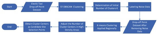
Figure 1.
GPS trajectory point clustering process.
2.1.1. Drop-Off Point Clustering Based on ST-DBSCAN
The ST-DBSCAN algorithm [30] is an enhanced density-based spatiotemporal clustering method that builds upon the traditional DBSCAN by incorporating multidimensional attributes—such as geographic coordinates, timestamps, speed, and movement direction—of trajectory points. This integration allows for a more accurate representation and clustering of moving object behaviors. Compared with the standard DBSCAN algorithm, which relies solely on spatial distance, ST-DBSCAN significantly improves the expressiveness of data attributes, the identification of noise points, and the evaluation of boundary point densities, thereby enhancing overall clustering accuracy.
The traditional DBSCAN algorithm groups data points into clusters based on spatial distance similarity, by identifying regions where the number of points within a given radius exceeds a predefined density threshold. ST-DBSCAN builds upon this framework by simultaneously incorporating temporal attributes and non-spatial features [30]. It models the time axis as a linearly increasing function, enabling the calculation of spatiotemporal distance with a solid theoretical foundation. Additionally, ST-DBSCAN introduces the concept of a density factor to dynamically adjust the boundary density threshold of clusters, effectively addressing the issue of misclassifying noise and boundary points in datasets with uneven density distributions. By comparing the average density within a cluster to the locally recalculated density, the algorithm further refines cluster boundaries, thereby enhancing its adaptability and clustering quality under complex mobility patterns.
In the clustering analysis of electric taxi drop-off points, ST-DBSCAN emphasizes two core attributes: space and time. It evaluates the density distribution of drop-off points based on the constructed spatiotemporal neighborhoods.This quantification of spatiotemporal density provides a reliable basis for the division of clusters, which achieves a reasonable classification and optimization of drop-off points.
Definition 1.

Spatiotemporal neighborhood. For any drop-off point in the trajectory point dataset S, its spatiotemporal neighborhood is illustrated in Figure 2. This neighborhood resembles a cylindrical region, where the radius of the base is defined by the spatial threshold parameter , and the height is determined by the temporal threshold . This cylindrical range captures nearby points that are not only spatially close to but also occur within a specific time window, enabling effective clustering of spatiotemporally correlated data.
Figure 2.
Spatiotemporal neighborhood of stay points.
In the above equation, represents the spatial distance and temporal distance between and q, respectively.
The set of drop-off points within the spatiotemporal neighborhood of is represented as follows:
Definition 2.
Spatiotemporal density. For any given drop-off point , its spatiotemporal density is defined as the number of drop-off points contained within the specified time and spatial thresholds, i.e., . Specifically, spatiotemporal density represents the total number of drop-off points whose spatial distance from the current drop-off point is less than the set spatial threshold and whose time difference is smaller than the set time threshold.
2.1.2. Determination of the Number of Charging Piles for Electric Taxis Based on Drop-Off Point Clustering
The K-means clustering algorithm [31] is a classical partition-based method characterized by its generation of spherical clusters. It achieves clustering by minimizing the intra-cluster distances while maximizing the inter-cluster distances, thereby satisfying the optimization criterion for clustering. Owing to its high computational efficiency and strong performance in finding local optima, the K-means algorithm is widely applied in trajectory data analysis and hotspot detection. Leveraging these advantages, this section employs the K-means algorithm to extract the centroid of each cluster obtained from the ST-DBSCAN results as the candidate location for charging stations.
In order to satisfy the charging needs of most electric taxi drivers, the number of drop-off points per unit of time is collected based on the resultant data after clustering the drop-off point data in the previous subsection, using a time resolution of one hour. The number of charging piles at charging station i is denoted as follows:
In the above equation, represents the number of drop-off points at charging station i during the t-th time interval, and is the peak-time immediate charging demand satisfaction coefficient.
2.2. System Design
The proposed PSCS consists of PV panels, ESSs, EVs, and the national grid. The primary power supply is provided by PV energy generation and ESSs to meet the vehicle charging needs, while backup power is supported through a connection to the national grid. The station is designed to maximize the use of renewable energy sources to ensure the stability and flexibility of the energy supply, and to supplement power through the grid when necessary for efficient energy management and deployment.
The charging stations are centrally regulated by the Energy Management Control Center, which coordinates power generation, transmission, and dynamic interaction with the grid to ensure the efficient and orderly operation of the station. The functions of each component of the charging station will be elaborated in the following sections.
- The PV panels are connected to the battery through a DC/AC module, which converts the generated energy into AC power via a charge controller for storage in the ESS.
- The battery is connected to the PSCS via a DC bus, enabling it to store the energy generated by the PV panels and supply power to EVs.
- The EV charging unit facilitates the transfer of electrical energy from the ESS and the utility grid into the EVs.
- The utility grid serves as a backup energy source for the charging station. When the energy stored in the battery is insufficient to meet the charging demand of EVs, the station directly purchases electricity from the grid to maintain supply–demand balance.
2.2.1. Modeling of PV Generation Unit
PV generation is directly influenced by meteorological conditions, especially fluctuations in solar irradiance. To improve the efficiency of solar energy utilization and support sustainable development, it is essential to systematically analyze and quantify these environmental factors. Considering the stochastic variability and time-dependent characteristics of solar resources, this section presents a modeling approach for PV power generation, aiming to accurately evaluate its output capacity and provide a reliable foundation for power generation forecasting.
Assuming that the behavior of solar irradiance follows a Beta probability distribution function [32], the probability density function of solar irradiance varying with time t is calculated as shown in Equation (3):
where represents the solar irradiance at time t; and denote the shape and scale parameters of the Beta function, respectively. In this study, the shape and scale parameters of the Beta function are set to 2.57 and 1.6, respectively [33].
In addition, the PV generation calculated using the generated irradiance values is shown in Equation (4):
where represents the PV generation under solar irradiance , kW; k denotes the efficiency of the PV panel; is the area of the installed PV panel, m2; is the solar irradiance at time t, in kW/m2; is the cell temperature of the PV panel, °C.
2.2.2. ESS Model
In the PSCS, the ESS is used as an energy storage unit to balance power supply and demand. The optimization model aims to determine the optimal capacity of the ESS and its charge/discharge schedule. The mathematical expression of the energy stored in the ESS at each time interval is given by Equation (5):
where represents the amount of energy stored in the ESS at t. is the self-discharge rate. and denote the charging power and charging efficiency at t, respectively. and denote the discharging power and discharging efficiency at time t, respectively. is the time interval.
As shown in Equation (6), at the initial and final hours, the energy should be the same to prevent energy accumulation.
The charging and discharging rates of the ESS are also subject to certain limitations and cannot exceed the rated power specified by the manufacturer.
where denotes the rated power.
2.3. Capacity Optimization Model for PSCS
The sets, parameters, and decision variables in the model are shown in Table 1 below.

Table 1.
Tables of sets, parameters, and decision variables.
This section develops a bi-variable optimization model with the number of PV panels and the number of batteries as decision variables, aiming to minimize the total cost F. The total cost comprises two components: (1) the upfront investment cost for PV panels and batteries and (2) the operational cost of purchasing electricity from the grid. By jointly considering these cost components, the model seeks to optimize the economic efficiency of resource allocation.
The optimization objective is shown in the following equation:
The constraints are shown below:
Constraints (13) and (14) represent the upfront investment costs for PV panels and ESSs, respectively; Constraint (15) is used to calculate the charging load of the station at time t; based on this temporal load profile; Constraint (16) further computes the annual cost of electricity purchased from the grid; and Constraint (17) defines the amount of electricity procured from the grid at time t.
3. Algorithms
3.1. Clustering Algorithm-Based Solution for Siting and Capacity Planning
The first stage of the model addresses the classical coverage localization problem [34], which is NP-hard and computationally intractable for large-scale instances. To overcome this, we exploit the spatiotemporal distribution of charging demand using a two-stage clustering approach.
First, the ST-DBSCAN algorithm identifies high-density demand regions by clustering charging events in both space and time, effectively capturing typical usage patterns such as commuter peaks in residential or commercial areas. As ST-DBSCAN may produce irregular cluster shapes and imprecise centroids, we further apply K-means within each cluster to refine station sites by minimizing intra-cluster distances.
Based on the final cluster centers, we extract the hourly demand profile over a 24-h period for each candidate site. The number of required charging piles is then determined using the peak hourly demand and a given satisfaction coefficient, ensuring adequate service capacity at each station.
The algorithm for its solution is as Algorithm 1.
| Algorithm 1 ST-DBSCAN + K-means for charging station siting |
| Input Data: Charging demand dataset where: • Location: • Timestamp: Parameters: • ST-DBSCAN: , , MinPts • K-means: K (number of clusters) • Charging coefficient: Initialize: • Mark all as unvisited • cluster_id , noise • Initialize empty cluster set for each unvisited point do Mark as visited if then Label as noise else cluster_id ← cluster_id + 1 Create new cluster ExpandCluster(, , ) for each cluster where do Randomly select K initial centers repeat Assign each to nearest center Update centers: until cluster assignments stabilize Compute peak hourly demand: Calculate required charging piles: Output: • Optimal selections: for each qualified cluster • Demand point sets: for all clusters • Required charging piles: per selection |
3.2. Genetic Algorithm (GA)-Based Solution for PSCS Capacity Optimization
Because the capacity optimization model for PSCS involves nonlinear relationships between the number of PV panels () and battery units (), as well as their impact on grid electricity consumption, solving it analytically becomes computationally intensive. To address this complexity, we adopt a GA to efficiently search for near-optimal solutions.
Before presenting the algorithm in detail, we briefly outline the rationale. The objective is to minimize the total cost of installing and operating PV panels and ESSs at each charging station. This cost includes both the capital investment in hardware and the cost of purchasing electricity from the grid, which is influenced by the PV output and battery discharge over a 24-h period. The optimization is further complicated by the time-varying nature of charging demand and the stochastic state-of-charge (SOC) of incoming vehicles.
To handle these nonlinearities, the GA iteratively evolves a population of candidate configurations. Each individual in the population represents a pair . The fitness of each individual is evaluated based on the total daily cost. Standard evolutionary operators such as selection, crossover, and mutation are applied to guide the population toward lower-cost solutions. This evolutionary strategy allows the model to flexibly explore the complex decision space without relying on gradient information or convexity assumptions.
The detailed steps of the GA-based optimization are provided in Algorithm 2.
| Algorithm 2 GA for PV panel and battery selection |
| Input: • Charging stations with charging pile counts • Cost parameters: , , , • GA parameters: Population size M, generations G, crossover prob. , mutation prob. , mutation range Initialize: • Population random individuals (size M) • Generation counter while do for each station and hour do Sample initial SOC: , clipped to Compute load: for each individual do PV output: Battery power: Grid power: Total cost: Fitness: Sort by ascending fitness Select parents via tournament selection Crossover (prob. ): child Mutation (prob. ): , Form new population Update best solution: Output: • Optimal configuration: • Minimum cost: |
4. Case Study
The spatiotemporal trajectory data generated by electric taxis during daily operations provide crucial support for the charging station siting methodology proposed in this study. As a form of individual-level spatiotemporal big data, taxi GPS records are extensively used in contemporary research due to their high continuity, reliability, and the abundance of publicly available resources. For electric taxi studies, the primary authoritative public dataset is the Shenzhen taxi trajectory dataset, released by the research group of Assistant Professor Desheng Zhang at Rutgers University, USA. This dataset comprises over 40 million trajectories collected from 14,728 vehicles in a single day, with passenger-loaded trajectory data totaling 1.74 GB [35]. Consequently, Shenzhen is chosen as the case study region for validation.
4.1. Siting and Capacity Configuration Results of PSCS
In this section, the charging demand selections of electric taxis are approximated as popular travel areas for Shenzhen residents. The core objective is to analyze the spatial and temporal distribution characteristics of drop-off points within the spatiotemporal trajectory data of electric taxis and to reveal their aggregation patterns. This analysis ultimately supports the determination of optimal charging station selections.
After an in-depth analysis and filtering of attributes such as latitude, longitude, timestamp, and speed within the trajectory dataset—as well as the processing of redundant, missing, offset, and anomalous data—the specific spatial distribution of drop-off points is obtained, as illustrated in Figure 3.
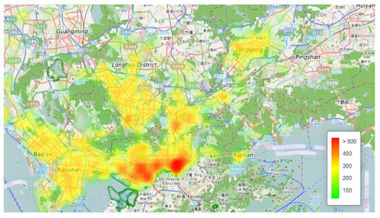
Figure 3.
Heat map of drop-off point distribution.
4.1.1. Charging Station Siting Results
In this paper, the spatial threshold , temporal threshold , and MinPts parameters for the ST-DBSCAN algorithm are set to 1000 [36], 120 [37], and 8 [38], respectively. The clustering process was executed on a standard workstation and completed in approximately 37 min. After filtering out 1087 noise points, a total of 21 spatiotemporal clusters were identified, with their spatial distribution illustrated in Figure 4.

Figure 4.
ST-DBSCAN clustering results (before filtering).
Subsequently, clusters with fewer than 10 dwell points are filtered out, resulting in 15 final clustering centers, as shown in Figure 5. Compared with the original dwell point data, these centers effectively cover areas with dense spatiotemporal distributions, while scattered points are treated as noise and excluded. This approach prevents clustering centers from deviating from high-density areas.The clustering results reveal significant differences in dwell point densities across the clusters. One cluster alone accounts for nearly 70% of all dwell points, whereas the sparsest cluster contains only 11 points. Spatially, the clustering centers are mainly concentrated in Nanshan and Bao’an Districts, with only one cluster located in Futian District. This is attributed to the uneven data distribution in Futian, where ST-DBSCAN fails to adequately identify high-density areas. Therefore, K-means algorithm optimization is applied to enhance site selection in Futian District.
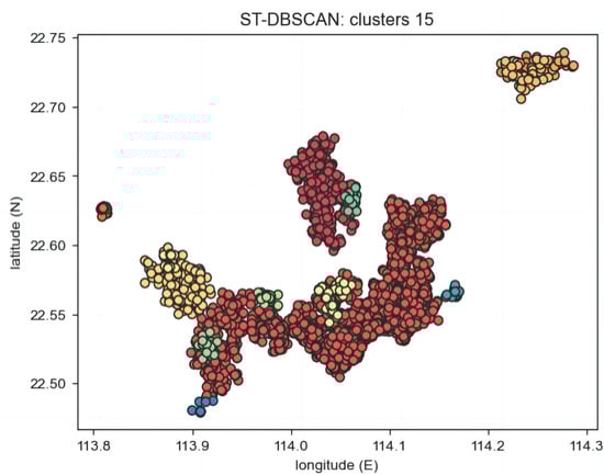
Figure 5.
ST-DBSCAN clustering results (after filtering).
To further refine the station siting process and account for intra-cluster variation in dwell point density, we analyze the distribution characteristics of each identified cluster. Among these clusters, Class Cluster 3 exhibits a significantly higher distribution density. Therefore, based on the elbow method, its K value is set to 6, while the K values for the remaining clusters are set to 1. As a result, a total of 20 charging station siting points are determined, with their spatial distribution illustrated in Figure 6.
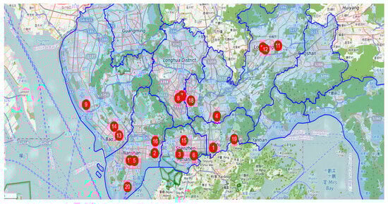
Figure 6.
Distribution of charging station site selection results. (Note: The numbers in the red circles represent site identifiers, which are consistent with the numbering in Figures 10, 14, and 15).
From the above site selection results, it is evident that the strategy effectively considers both dwell point density and regional charging demand. This can be seen in the distribution of stations, where most stations are concentrated in central urban areas like Bao’an, Longgang, Futian, and Nanshan. For example, Nanshan hosts five stations: 2, 5, 16, 17, and 20. These locations, often in high-demand areas, not only meet taxi charging needs but also improve charging convenience during passenger activities, enhancing operational efficiency.
4.1.2. Charging Piles Allocation
After determining the selections of the charging stations, a spatiotemporal analysis of the ST-DBSCAN clustering results was conducted to better meet the charging demands of electric taxis, enhance driver satisfaction, and enable timely response to charging needs. Specifically, the drop-off point data within each cluster were aggregated by hourly intervals to reveal the temporal distribution patterns of taxi drop-offs over a 24-h period. As illustrative examples, the temporal distribution patterns for Site 1, Site 10, and Site 13 are shown in Figure 7, Figure 8, and Figure 9, respectively.
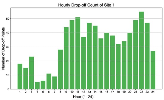
Figure 7.
Distribution of drop-off point counts at site 1.
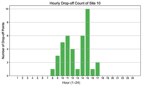
Figure 8.
Distribution of drop-off point counts at site 10.

Figure 9.
Distribution of drop-off point counts at site 13.
From the time distribution of single-day (weekday) drop-off points, Site 1, located in Luohu District, exhibits high-frequency travel between 8:00 and 23:00, with a peak occurring around 22:00 and minimal activity during the early morning hours. This pattern closely mirrors the typical daily travel behavior of residents in the area. Site 10, situated in Longgang District—a region characterized by the presence of factories, office buildings, and schools—shows travel demand primarily concentrated during daytime hours, aligning with the working and schooling schedules of the local population. Site 13, located in Nanshan District, demonstrates a travel peak in the evening, attributed to the abundance of recreational facilities in the vicinity. This spatiotemporal pattern reflects the functional characteristics of the district.
Based on the above temporal demand distributions, the number of charging piles allocated to each charging station can be determined using the method described in Section 2. The specific scale of allocation is illustrated in Figure 10 below.
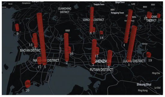
Figure 10.
Charging pile scale. (Note: The horizontal lines represent the height of a single charging pile, and the number of layers reflects the total number of piles at each station).
From the above charging pile allocation results, the strategy effectively optimizes infrastructure layout and service efficiency based on demand distribution. Specifically, in districts like Bao’an, Luohu, Futian, and Nanshan, the high density of drop-off points correlates with increased charging pile deployment at local stations. This distribution mirrors the spatial patterns observed in raw taxi trajectory data, where charging demand naturally concentrates in densely populated, high-traffic areas.
4.2. Electric Taxi Demand Simulation
The primary service targets of the proposed PSCS are electric taxis. The charging station load is simulated based on the number of drop-off points at each station. It is assumed that the initial SOC of each electric taxi arriving at the station follows a normal distribution . By combining this with the number of drop-off points obtained from the hourly post-processed clustering results, and assuming a probability of 0.8 that a taxi will proceed to charge, the corresponding electricity demand load profiles can be generated. These are illustrated in Figure 11, Figure 12 and Figure 13, using Stations 1, 10, and 13 as examples.
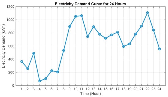
Figure 11.
Charging demand load map for site 1.
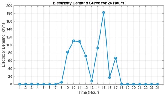
Figure 12.
Charging demand load map for site 10.

Figure 13.
Charging demand load map for site 13.
4.3. Results of PV and Battery Capacity
The model parameters (Table 2) and GA settings (Table 3) are as follows. The GA was used to solve the optimization model ten times for each site, and the target minimum was selected from the ten results as the required PV panels and batteries for each site. The results are presented in Figure 14 and Figure 15, with detailed numerical data summarized in Table 4.
Table 2.
Model parameters.
Table 3.
GA parameters.
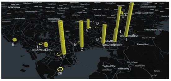
Figure 14.
Distribution of the number of PV panels at each site. (Note: The horizontal lines represent the height of a single PV, and the number of layers reflects the total number of PV at each site).
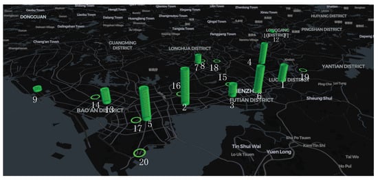
Figure 15.
Distribution of the number of batteries at each site. (Note: The horizontal lines represent the height of a single battery, and the number of layers reflects the total number of battery at each site).
Table 4.
Quantity of equipment configuration at charging stations.
In the following, we observe the rationality of the PV module configuration from two perspectives: first, whether the scale of PV panel and battery configuration aligns with the corresponding level of charging demand; and second, whether the ratio between PV and storage system configurations remains fixed or varies according to the structure of the charging demand. We obtain the following conclusions:
(1) Configuration levels are generally in line with demand levels. Overall, the number of PV panels and batteries is positively correlated with the charging demand at each site. Selections with higher demand are typically equipped with more PV panels and batteries, whereas sites with lower demand require fewer components. For instance, Site 8 is situated in an area with a relatively high level of demand and is therefore configured with a greater number of PV panels and storage units. In contrast, Site 13 experiences lower demand, necessitating only minimal equipment to satisfy its operational requirements.
(2) The ratio of PV to battery allocation varies according to the charging demand structure, showing a non-fixed characteristic. For instance, although Site 2 and Site 4 have similar total configurations, their PV-to-battery ratios differ noticeably. Analyzing the configuration results reveals that the allocation of PV panels and batteries is influenced by the temporal distribution of charging demand. Site 2 is located in an area with high daytime charging demand and relatively low nighttime usage, making it suitable for meeting energy needs directly through PV generation. Consequently, it is configured with more PV panels and fewer batteries (48:31). In contrast, Site 4 experiences a higher load during nighttime hours, requiring greater reliance on battery storage to ensure power supply after sunset. As a result, it is equipped with more batteries and slightly fewer PV panels (51:22). These differences demonstrate that the diurnal characteristics of charging demand play a significant role in determining the optimal PV-to-battery configuration ratio.
Overall, the allocation ratio of PV panels to storage should be flexibly adjusted according to the actual demand structure of each site. In this study, the observed ratio ranges approximately from 1.5:1 to 0.5:1, reflecting a strategic adjustment driven by load characteristics. Specifically, sites with predominantly daytime charging demand tend to be equipped with a higher number of PV panels, while those with significant nighttime demand emphasize increased storage capacity. This demand-driven configuration enhances the synergy between PV generation and energy storage systems, thereby improving overall system operational efficiency and ensuring a more reliable power supply.
4.4. Analysis of Typical PSCS
While the above is an overall analysis of PV panels and battery configuration models, this section will focus on equipment configurations and cost analysis for typical PSCS with different demand types, using Sites 1, 10 and 13 as examples.
(1) All-day Load-type Sites (Site 1)
At Site 1, the EV charging demand is distributed throughout the entire day, with a pronounced surge between 08:00 and 24:00, peaking at 23:00. As illustrated in Figure 16 and Figure 17, the total energy supply at this site largely aligns with the load demand. Notably, the PV accounts for 58% of the total electricity supply. Of this, 2.2% is stored in batteries during peak generation hours and discharged between 16:00 and 19:00 to support EV charging. The remaining 42% of the demand is met by the power grid. During periods of high solar irradiance—especially from 12:00 to 16:00—PV generation is sufficient to fully cover the charging demand, and excess power is directed to battery storage. As irradiance decreases in the evening, PV output declines, prompting the system to discharge stored energy. If the battery output is insufficient, the system switches to grid power to meet the remaining demand. These findings suggest that in cases of strong and continuous daily charging demand, the system tends to favor a larger PV configuration, enabling solar energy to play a leading role in supplying the charging load. This not only reduces dependence on grid electricity but also supports cost-effective and sustainable energy utilization.
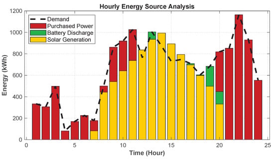
Figure 16.
Site 1—energy source analysis diagram.
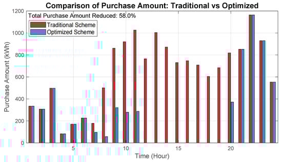
Figure 17.
Site 1—power purchase comparison chart.
In addition, Figure 18 shows the results of the purchased power versus the annualized total cost for Site 1 with and without the PV system. In the traditional scenario, the system is completely dependent on the grid for power supply, while the optimized scenario achieves local power supply for part of the load by introducing PV modules. The results show that the annualized total cost of the optimized scenario is reduced by 13.4% compared to the traditional scenario, in which the purchased power cost is reduced from RMB 2,835,000 to RMB 1,191,000, which is a significant improvement in economy.
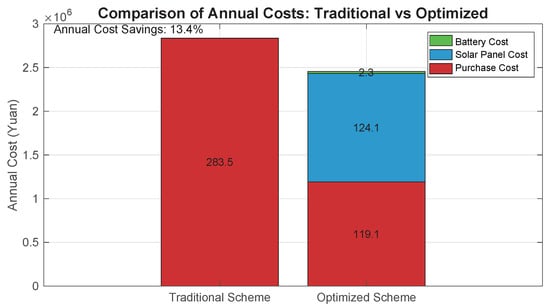
Figure 18.
Site 1—cost comparison chart.
(2) Daytime-dominated Sites (Site 10)
The energy distribution of Site 10 is shown in Figure 19 and Figure 20. For this site, where the charging demand is mainly concentrated during daytime hours, the energy allocation strategy tends to prioritize increasing the installation size of PV panels while reducing the number of batteries. However, due to the overall low level of charging demand at this site, the number of PV panels configured is significantly lower than that at high-load sites. During the daytime peak load period, the PV system undertakes most of the energy supply task, with an energy supply ratio of 66.9%, effectively meeting the immediate load demand and greatly alleviating the pressure on the grid power supply. Nevertheless, due to the limited capacity of the PV system, its generation is still insufficient to fully cover the entire demand gap.
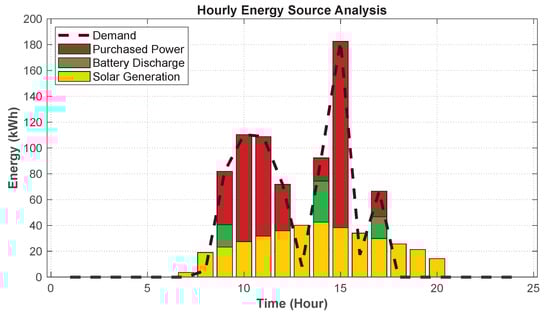
Figure 19.
Site 10—energy source analysis diagram.
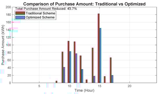
Figure 20.
Site 10—power purchase comparison chart.
Figure 21 further demonstrates the results of the site’s power purchase versus annualized total cost before and after the deployment of PV modules. The results show that the cost of purchased electricity was significantly reduced from RMB 136,000 to RMB 77,000 after the introduction of the PV system. The main reasons for this are as follows: on the one hand, the overall charging load at Site 10 is low, so even if it relies entirely on grid power, the purchased power cost is relatively small; on the other hand, the higher initial investment cost of the PV system is difficult to be fully amortized in low-load scenarios, which results in limited room for economic improvement.
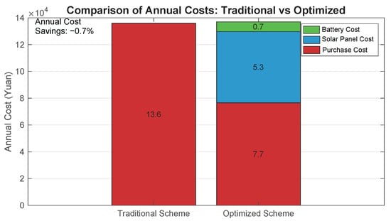
Figure 21.
Site 10—cost comparison chart.
(3) Nighttime-dominated Sites (Site 13)
The energy distribution at Site 13 is shown in Figure 22, Figure 23 and Figure 24. For sites where charging demand is mainly concentrated in the evening and nighttime, the configuration strategy favors increasing the capacity of the batteries, while the number of PV panels configured is relatively small. The core of this configuration scheme is to utilize the PV power generation during the daytime when there is sufficient light and store the power in the battery for release in the evening or nighttime when there is insufficient light, so as to provide energy security for electric taxis. The results of the system optimization show that the annual purchased power at Site 13 is reduced by 21.3% after the deployment of the PV modules, alleviating the dependence on the grid to a small extent. However, the reduction in total system cost is more limited at 2.4% compared to the significant reduction in purchased power.

Figure 22.
Site 13—energy source analysis diagram.
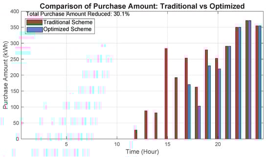
Figure 23.
Site 13—power purchase comparison chart.

Figure 24.
Site 13—cost comparison chart.
This phenomenon is mainly due to a combination of several factors. First, the discharge capacity of the batteries is constrained by their storage time and efficiency. As the main load of Site 13 is concentrated in the evening to night, after discharging during the day, the battery cannot complete the charging and re-discharging process in a short period of time, making it difficult to fully cover the continuous growth of the load demand at night and still requiring supplemental energy from the grid. Second, the battery itself has a capacity limit and high investment cost, which largely limits the feasibility of its large-scale configuration. Although theoretically increasing the number of batteries can further reduce the demand for electricity, the corresponding cost will rise significantly, affecting the overall economic efficiency.
In this section, the energy allocation strategies and operational effectiveness of PSCS under different charging demand characteristics are analyzed using Sites 1, 10, and 13 as representative cases. The analysis highlights the profound impact of both the temporal distribution and intensity of load demand on system configuration and economic performance. The key findings are as follows:
- The temporal characteristics of charging load are critical determinants of the PSCS configuration strategy. For all-day load-type sites (e.g., Site 1), where charging demand spans both daytime and nighttime, the PV system and energy storage devices operate synergistically. This coordination enables high utilization of renewable energy and yields favorable economic outcomes. In contrast, for daytime-dominated sites (e.g., Site 10), the PV system can directly meet peak demand during high irradiance hours, effectively reducing reliance on grid power. However, the improvement in total cost remains limited due to the relatively low overall load level. For nighttime-dominated sites (e.g., Site 13), although part of the load can be shifted by deploying energy storage, the economic benefits of storage are difficult to realize due to the significant mismatch between PV generation capacity and nighttime demand. As a result, the reduction in total system cost is constrained.
- The overall charging load level plays a decisive role in determining the return on system investment. At high-load sites, the higher utilization rates of PV panels and ESSs contribute to spreading out the initial investment costs over a larger energy output, thereby significantly enhancing the overall economic efficiency. Conversely, at low-load sites, although a higher proportion of the energy supply may come from local sources, the return on investment per unit of capacity is prolonged, and the potential for economic improvement remains limited.
In conclusion, the optimal design of PSCS must carefully account for both the temporal distribution characteristics and the scale of the charging load. Achieving efficient coordination between the PV, ESS, and grid power is essential.
5. Sensitivity Analysis
After calculating the above example, in order to identify the key factors affecting the model, a sensitivity analysis was performed next to extract three important parameters: peak instantaneous service satisfaction of electric taxi demand and cost of PV and battery.
5.1. Peak Instantaneous Satisfaction Rate () of Demand for Electric Taxis
The is a direct reflection of the service quality of the charging station, indicating the probability that a user will receive instant service when the station is most congested, thus ensuring a minimum quality standard of service. At the same time, the loss rate has a direct impact on the revenue of the operator, who seeks to maximize the number of vehicles served while maintaining a certain level of service quality. is closely related to loss rate, but they are not identical.
For example, under the same , for charging stations with smooth demand, the overall vehicle loss rate roughly matches 1 − , and the charging pile utilization rate is higher. For charging stations with fluctuating demand, the loss rate is often much lower than 1 − , resulting in lower utilization of charging piles, which directly affects the operator’s revenue.
This section sets the waiting time for charging that is acceptable to users at 1 h, meaning users who fail to charge within 1 h will choose to leave, leading to a loss of customers. As a result, the number of charging piles cannot be determined by simply relying on the satisfaction rate during peak hours. A more reasonable resource allocation should be made by comprehensively considering the spatial and temporal distribution characteristics of charging demand, the utilization rate of charging piles, and the overall operational efficiency of the station.
Therefore, this study conducts a sensitivity analysis of the instantaneous charging satisfaction rate during peak periods for representative stations with different demand scales, using Station 1 and Station 13 as case studies. The specific analysis is presented below.
(1) Impact Analysis for Site 1
Figure 25 shows the changes in the number of station facilities and total cost for Site 1 (all-day loaded site) under different . When the is 50%, the numbers of charging piles, PV panels, and batteries are 22, 41, and 7, respectively. As the increases, the numbers of charging piles, PV panels, and batteries, as well as the total cost, show an upward trend, but there are variations in the magnitude of the growth across different facilities. In the process of increasing the from 50% to 80%, the increase in the number of PV panels is significantly higher than in the stage from 80% to 100%, while the growth trend of storage batteries shows the opposite change. This suggests that as the improves, the allocation of PV panels initially increases at a faster pace compared to storage batteries, but the trend reverses at higher satisfaction rates, with the battery allocation growing more gradually. This finding highlights the different roles that PV panels and storage batteries play in meeting the charging station’s operational requirements, with PV panels primarily addressing daytime demand and batteries helping to balance the energy supply during peak charging times.
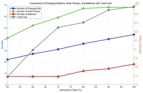
Figure 25.
Site 1—changes in facilities.
Figure 26 reveals the trend in loss rate at different for Site 1. Initially, when the is 50%, the vehicle loss rate reaches a high level of 79.31%. As the increases, more charging piles are configured, the total number of vehicles served rises, and the number of vehicles that fail to receive charging services—i.e., the loss rate—decreases significantly. When the reaches 100%, all vehicle charging needs can be fully met, effectively eliminating loss. The figure further illustrates that the most substantial drop in loss rate occurs as the increases from 50% to 80%, whereas the rate of decline slows considerably in the 80% to 100% range. This trend suggests diminishing returns in loss reduction as the station approaches full satisfaction. Therefore, in balancing cost and service efficiency, configuring Site 1’s facilities to achieve approximately 80% satisfaction appears to be the optimal point—ensuring relatively high service quality while maintaining economic feasibility.
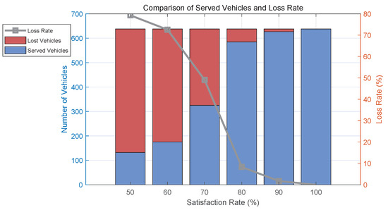
Figure 26.
Site 1—changes in satisfaction rates.
Figure 27 illustrates in greater detail how variations in the affect the number of vehicle loss per hour. For a site like Site 1, characterized by an uneven demand distribution throughout the day, increasing the from 50% initially reduces vehicle loss most significantly during the peak hour at 22:00. Additionally, a substantial decrease in vehicle loss is observed during daytime hours, while the change in demand loss during nighttime remains relatively limited. This stage is accompanied by a more pronounced increase in the number of PV panels compared to battery units. However, when the increases from 80% to 100%, the reduction in the number of vehicles failing to receive charging services is more pronounced during nighttime hours, whereas the change during the daytime is relatively limited.
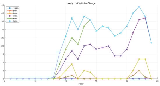
Figure 27.
Site 1—Vehicle Loss per Hour Comparison Chart.
(2) Impact Analysis for Site 13
Figure 28 illustrates the relationship between station facility configurations and service efficiency for Site 13 (a centralized nighttime site) under varying . Due to the concentration of charging demand during nighttime hours, changes in the have a more pronounced impact on battery configuration than on PV panel allocation. Nonetheless, the overall trends in the configurations of PV panels and batteries are similar: during the phase where the increases from 50% to 70%/80%, there is a significant rise in facility deployment. However, as the continues to rise from 80% to 100%, the growth in facility numbers slows down considerably, with the number of PV panels even tending to stabilize, indicating no further increase.
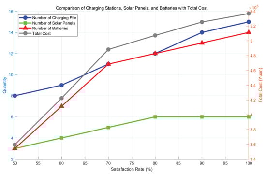
Figure 28.
Site 13—changes in facilities.
Figure 29 further reveals the variation in the charging demand loss rate at different for this site. As the increases from 50% to 70%, the loss rate drops significantly from 74.60% to 19.05%, indicating a substantial enhancement in charging service capacity. To observe the improvements across different time periods more precisely. Figure 30 analyzes the temporal distribution of the number of lost vehicles. During the stage where the increases from 50% to 70%, the number of missed vehicles between 15:00 and 24:00 is significantly reduced, demonstrating improved service capability during this period. As the continues to rise from 70% to 100%, changes in the number of lost vehicles are mainly concentrated after 20:00, highlighting that service capacity during the late-night peak still faces limitations. More specifically, when increasing the from 70% to 80%, noticeable improvements are still observed between 15:00 and 20:00. However, in the 80% to 100% range, nearly all improvements in lost vehicle numbers occur after 20:00. This suggests that PV panel configuration may still slightly increase during the 70% to 80% stage, while remaining essentially unchanged from 80% to 100%. At this point, the burden of meeting the nighttime peak charging demand is primarily borne by expanding battery capacity. Nevertheless, compared to the 50% to 70% stage, the growth in battery deployment slows down in the 80% to 100% range, and the marginal benefit of further investment in energy storage diminishes.
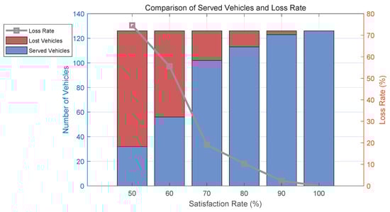
Figure 29.
Site 13—changes in satisfaction rates.
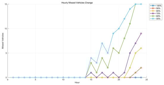
Figure 30.
Site 13—vehicle loss per hour comparison chart.
In summary, the above analysis demonstrates that stations with different charging demand profiles exhibit significantly distinct response mechanisms to variations in the . For all-day load-type stations, resource allocation must account for both daytime and nighttime service capabilities. This necessitates a flexible combination of PV panels and battery storage to address varying temporal demand pressures. In contrast, for stations with demand concentrated at night, batteries emerge as the critical resource to ensure nighttime service quality, with improvements in the primarily achieved through increased energy storage capacity. Therefore, in the planning and operation of charging infrastructure, it is essential to accurately identify the demand characteristics of each station. By coupling this understanding with the sensitivity of , a tailored resource allocation strategy can be developed to achieve an optimal balance between service efficiency and economic cost.
5.2. Cost of PV and Battery
To comprehensively evaluate the impact of cost fluctuations in PV panels and batteries on station economics and facility configuration, a sensitivity analysis was conducted in this study. Given the relatively high cost of PV panels, scenarios were designed with 10% and 20% increases and decreases in panel costs. In contrast, battery costs are comparatively lower, so a wider range of scenarios was considered, including 40%, 60%, and 80% cost increases, as well as 20% and 40% cost reductions.
To further explore the synergistic effects of concurrent cost variations in both PV panels and batteries, additional combined scenarios were examined, including the following:
- 10% increase in PV panel cost with a 20% increase in battery cost;
- 20% increase in PV panel cost with a 40% increase in battery cost;
- 10% decrease in PV panel cost with a 20% decrease in battery cost;
- 20% decrease in PV panel cost with a 40% decrease in battery cost.
These simulation and comparative analyses provide valuable insights and robust decision support for the optimal design and cost control of EVCS.
(1) Impact of Changes in PV panel Cost
As shown in Figure 31, rising PV panel cost significantly impacts high-demand sites like Site 1. As cost increases, the number of PV panels decreases from 86 to 59, and batteries from 79 to 6. This reflects higher upfront investment pressure, prompting sites to scale back PV installations to stay within budget—especially when the marginal gains from PV generation no longer offset the added cost. As PV capacity declines, generation-side volatility is reduced, leading to a sharp decrease in battery demand.
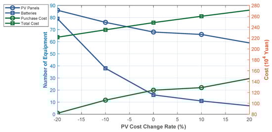
Figure 31.
PV panel cost-facility and cost change chart.
Figure 32 demonstrates the time-series impact of rising PV panel cost on station configuration. When cost increases slightly (baseline to +10%), the PSCS relies more on grid power and ESSs between 19:00 and 21:00, leading to higher electricity purchase costs. As cost rises further (+10% to +20%), daytime PV generation (07:00–12:00) also declines, further increasing grid dependence. The reduction in PV capacity prompts adjustments in ESS configuration. Initially, reduced PV output leads to increased ESS capacity to maintain service levels. When PV costs are low, the system minimizes ESS investment to control capital expenditure. However, as PV costs exceed the baseline, PV and ESS capacities begin adjusting in tandem to balance cost and performance. At higher cost levels (+20%), the system significantly reduces both PV and battery installations, shifting toward grid reliance as a cost-saving measure.
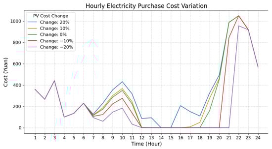
Figure 32.
PV panel cost—hourly purchased power cost change chart.
Figure 32 also shows that rising PV costs significantly increase total cost, driven by both higher equipment investment and electricity purchases. In contrast, cost reductions yield larger savings, indicating the system is more responsive to decreases than increases. Overall, higher PV panel costs reduce solar utilization, increase grid dependence, and undermine both sustainability and cost-effectiveness.
(2) Impact of Changes in Battery Cost
Figure 33 shows the battery cost sensitivity results for Site 1. As battery costs rise, the number of batteries deployed drops sharply, indicating the system reduces storage investment to control capital cost. When costs increase by 80%, battery deployment nearly ceases, reflecting a shift toward grid reliance. In contrast, PV panel configurations remain largely stable regardless of battery cost changes. This suggests that PV investments are prioritized and relatively insensitive to battery pricing, highlighting their central role in the system’s energy strategy.
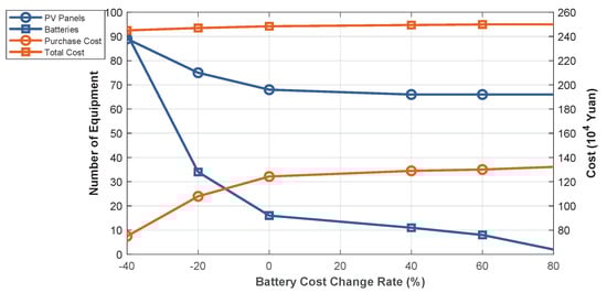
Figure 33.
Battery cost-facility and cost change chart.
Figure 34 illustrates how changes in battery cost affect system configuration. As costs rise from −40% to the baseline, noticeable shifts occur in energy supply during 7:00–12:00 and 18:00–23:00. To reduce capital investment, the system cuts back on batteries, which, in turn, limits ESS capacity. To avoid excess solar energy that cannot be stored, PV installations are also reduced. However, the limited storage weakens load-shifting capability, increasing reliance on grid electricity. As a result, savings in equipment cost are offset by higher power purchases, keeping total system cost nearly unchanged.
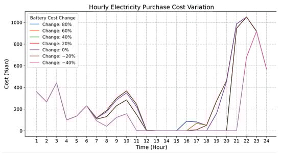
Figure 34.
Battery cost—hourly purchased power cost change chart.
As battery costs continue to rise, battery deployment further declines. Yet, increased power costs are balanced by reduced investment in storage, resulting in a relatively stable overall cost. This indicates that the system adapts its configuration to maintain economic efficiency and operational stability under high battery cost scenarios, with purchased power playing a key balancing role.
(3) Synergistic Impact of PV panel and Battery Cost Changes
Figure 35, Figure 36 and Figure 37 demonstrate the synergistic impact of PV panel and battery cost changes on the system configuration at Site 1. As the cost of PV panels and batteries decreases (e.g., from +20% and +40% to the baseline values), the number of PV panel configurations increases from 59 to 68, while the number of batteries increases to 16 sets, a relatively small change. However, when the cost continues to decline, the configuration changes become more pronounced: the number of PV panels rises substantially to 108 units, and battery configurations increase markedly to 187 units. This highlights the strong responsiveness of system design to cost reductions, particularly when both components become significantly more affordable.
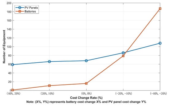
Figure 35.
Synergies with changes in equipment cost—number of pieces of equipment.
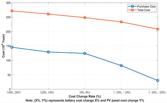
Figure 36.
Synergy of equipment cost changes—cost changes.
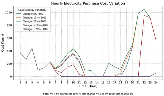
Figure 37.
Synergies in equipment cost changes—purchased power cost per hour.
This change indicates that as the cost of PV panels decreases, the system tends to increase PV panel installations to maximize the utilization of solar energy. Simultaneously, due to the relatively lower cost of batteries, the system significantly expands battery capacity to enhance energy storage and reduce dependence on grid electricity. With the expansion of the ESS, a larger share of the energy demand can be met by the PV-ESS, thereby reducing grid reliance. Consequently, the cost of purchased electricity drops markedly from RMB 1,242,682.38 to RMB 301,531.14, while the total system cost declines from RMB 2,483,911.98 to RMB 2,084,927.46. These results demonstrate that low-cost equipment configurations can effectively lower electricity purchase expenses, thus reducing overall cost. However, the reduction in total cost is less pronounced than the decline in power purchase cost, primarily because the savings in electricity expenses are partially offset by increased investment in system equipment.
The above sensitivity analysis reveals that changes in the cost of PV panels and batteries have a significant influence on system configuration and economic performance. In single-cost scenarios, fluctuations in the PV panel cost exert a more direct impact on system configuration, primarily determining the share of renewable energy supply and the level of self-sufficiency during daytime hours. In contrast, battery cost variations mainly affect the system’s nighttime operation strategy and load balancing during peak demand periods. In synergistic cost-change scenarios, the system exhibits a more pronounced coupling response: when both PV and battery cost decrease simultaneously, the system tends to adopt large-scale integrated PV-ESS configurations, significantly enhancing energy self-sufficiency and operational resilience. Conversely, when the costs of both components increase, the system progressively shifts toward greater reliance on grid electricity to contain total expenditures, reflecting a clearly cost-driven configuration strategy.
6. Conclusions and Outlook
6.1. Conclusions
In this paper, a siting and capacity optimization method for integrated PSCS, which considers the spatiotemporal distribution of charging demand, is proposed based on the GPS trajectory data of electric taxis in Shenzhen. The proposed approach involves constructing a two-stage framework: a siting model based on spatiotemporal clustering (ST-DBSCAN and K-means) and a capacity configuration model that accounts for the heterogeneous demand structure. A GA is used to solve the model and evaluate the economic and operational performance of different deployment strategies.
This study also addresses several key limitations in the prior research, especially in [28], where charging demand is modeled using aggregated station-level load profiles and uniform assumptions across functional zones. Specifically, reference [28] applies a fixed demand model for similar land-use types (e.g., hospitals, malls) across different regions, neglecting intra-zone variations in user behavior. In contrast, our data-driven approach utilizes high-resolution GPS trajectory data to reveal localized demand dynamics, enabling more precise and adaptive planning.
From a methodological standpoint, unlike previous studies [24,25,26,27] that optimize PV and ESS deployment from a grid-side—typically assuming uniform installation across all sites to enhance grid resilience—our model adopts an operator-side framework. It aims to minimize total cost while maintaining service reliability, allowing for selective deployment of resources based on localized demand profiles and investment feasibility. This shift in modeling logic leads to significantly different outcomes. For example, Sites 7 and 11 are identified as non-viable in our study due to insufficient returns under localized conditions, whereas prior grid-focused models would still mandate PV and ESS deployment at these locations.
Furthermore, most existing PSCS planning studies assume a fixed number of charging piles per station, focusing primarily on PV and ESS sizing without explicitly accounting for service-level performance. For instance, reference [39] assumes ten charging piles per site regardless of demand variations. Similarly, Castillo et al. [40] estimate charging pile requirements based on average daily traffic volumes without addressing peak-time fluctuations or queuing effects. Such simplifications risk underestimating congestion and lead to inefficient infrastructure use. In contrast, our study introduces a demand-responsive approach by determining charging pile counts as the product of peak-hour demand and (e.g., 80%). This explicitly integrates service quality into the planning process, balancing investment efficiency with user experience. Sensitivity analyses based on demand loss rates further validate this strategy. For example, Site 1 is configured to satisfy 80% of peak-hour demand, whereas 70% suffices for Site 13 due to its more evenly distributed load.
Using typical charging stations in Shenzhen as a case study, the following key conclusions are drawn from the sensitivity analysis on and equipment cost:
- The has a significant impact on both service level and system economics. As the volatility of charging load increases, the acceptable satisfaction threshold declines. By tailoring the number of stations to match the spatial demand distribution, the model effectively balances user satisfaction with equipment investment, enhancing overall economic viability.
- In high-demand areas, deploying more PV and ESS resources is economically justified to alleviate peak load stress. Conversely, in low-demand areas, reduced or no configuration is recommended to minimize cost. Since different urban functional zones exhibit distinct temporal charging profiles, the PV and storage capacity ratios should be jointly optimized according to area-specific energy usage patterns.
In summary, the proposed data-driven and demand-responsive framework offers a scientifically grounded and practically implementable solution for PSCS deployment. Due to the fundamental differences in demand acquisition and decision-making structure, this study is not directly comparable with earlier methods but rather represents a methodological advancement beyond their scope.
6.2. Limitations and Future Work
Although this study has achieved the expected results in exploring electric taxi charging station siting based on spatiotemporal trajectory data mining, there remains a gap between the current methodology and practical applications. Future research can be improved in the following three aspects:
- The solar irradiance data used in the current study are limited to a single representative day, which may not capture seasonal or weather-induced variations.Future work: Incorporate long-term historical meteorological data (e.g., spanning months or years) to improve the accuracy and robustness of PV power generation estimation.
- The energy cost model assumes a fixed electricity price and does not consider time-of-use pricing, which is widely adopted in real-world power markets.The model also does not include charge/discharge scheduling strategies for charging stations with energy storage, limiting the system’s flexibility.Future work: Introduce dynamic electricity pricing models and integrate charging/discharging scheduling strategies to better reflect operational realities and enhance economic performance.
- The ST-DBSCAN clustering algorithm demonstrates satisfactory performance on the current dataset of over 5572 demand points, with each complete clustering process taking approximately 27 min. This indicates the method’s computational feasibility for city-level planning. However, for larger-scale regions with more extensive data, the computation time is expected to increase roughly linearly. For example, when the number of demand points increases to 8840, the runtime extends to approximately 52 min.Future work: Explore more scalable and adaptive algorithms, such as reinforcement learning or surrogate-assisted optimization, to improve solution efficiency and quality in complex, real-world settings.
Author Contributions
Conceptualization, D.H. and D.Y.; methodology, D.Y.; software, D.Y.; validation, D.H. and D.Y.; formal analysis, D.H.; investigation, D.Y.; resources, D.Y.; data curation, D.Y.; writing—original draft preparation, D.H.; writing—review and editing, D.H., D.Y. and Z.-W.L.; visualization, D.Y.; supervision, D.H.; project administration, D.H.; funding acquisition, D.H. All authors have read and agreed to the published version of the manuscript.
Funding
This research is funded by National Social Fund of China grant 22BGL273.
Data Availability Statement
Dataset available on request from the authors.
Conflicts of Interest
The authors declare no conflict of interest.
References
- Ritchie, H.; Rosado, P.; Roser, M. CO2 and Greenhouse Gas Emissions. Our World in Data. 2023. Available online: https://ourworldindata.org/co2-and-greenhouse-gas-emissions (accessed on 17 April 2025).
- Thomas, C.E.S. How green are electric vehicles? Int. J. Hydrogen Energy 2012, 37, 6053–6062. [Google Scholar] [CrossRef]
- Lin, Q.Y.; Hong, Z.Y. Key technology design of integrated photovoltaic-storage-charging station. China New Telecommun. 2020, 22, 80. [Google Scholar]
- Fathabadi, H. Novel grid-connected solar/wind powered electric vehicle charging station with vehicle-to-grid technology. Energy 2017, 132, 1–11. [Google Scholar] [CrossRef]
- Karmaker, A.K.; Ahmed, M.R.; Hossain, M.A.; Sikder, M.M. Feasibility assessment & design of hybrid renewable energy based electric vehicle charging station in Bangladesh. Sustain. Cities Soc. 2018, 39, 189–202. [Google Scholar]
- Mouli, G.C.; Bauer, P.; Zeman, M. System design for a solar powered electric vehicle charging station for workplaces. Appl. Energy 2016, 168, 434–443. [Google Scholar] [CrossRef]
- Zhang, J.; Liu, C.; Yuan, R.; Li, T.; Li, K.; Li, B.; Li, J.; Jiang, Z. Design scheme for fast charging station for electric vehicles with distributed photovoltaic power generation. Glob. Energy Interconnect. 2019, 2, 150–159. [Google Scholar] [CrossRef]
- Hung, D.Q.; Dong, Z.Y.; Trinh, H. Determining the size of PHEV charging stations powered by commercial grid-integrated PV systems considering reactive power support. Appl. Energy 2016, 183, 160–169. [Google Scholar] [CrossRef]
- Satya Prakash Oruganti, K.; Vaithilingam, C.A.; Rajendran, G. Design and sizing of mobile solar photovoltaic power plant to support rapid charging for electric vehicles. Energies 2019, 12, 3579. [Google Scholar] [CrossRef]
- Rehman, A.U.; Ullah, Z.; Shafiq, A.; Hasanien, H.M.; Luo, P.; Badshah, F. Load management, energy economics, and environmental protection nexus considering PV-based EV charging stations. Energy 2023, 281, 128332. [Google Scholar] [CrossRef]
- Agbodjan, Y.S.; Liu, Z.Q.; Wang, J.Q.; Yue, C.; Luo, Z.Y. Modeling and optimization of a multi-carrier renewable energy system for zero-energy consumption buildings. J. Cent. South Univ. 2022, 29, 2330–2345. [Google Scholar] [CrossRef]
- Yang, M.; Zhang, L.; Zhao, Z.; Wang, L. Comprehensive benefits analysis of electric vehicle charging station integrated photovoltaic and energy storage. J. Clean. Prod. 2021, 302, 126967. [Google Scholar] [CrossRef]
- Yang, S.; Wu, M.; Jiang, J.; Zhao, W. An approach for load modeling of electric vehicle charging station. Power Syst. Technol. 2013, 37, 1190–1195. [Google Scholar]
- Hernández-Gómez, O.M.; Abreu Vieira, J.P. Probabilistic assessment of the impact of electric vehicle fast charging stations integration into MV distribution networks considering annual and seasonal time-series data. Energies 2024, 17, 4624. [Google Scholar] [CrossRef]
- Wang, S.; Liu, B.; Li, Q.; Han, D.; Zhou, J.; Xiang, Y. EV charging behavior analysis and load prediction via order data of charging stations. Sustainability 2025, 17, 1807. [Google Scholar] [CrossRef]
- Kim, S.; Hur, J. A probabilistic modeling based on Monte Carlo simulation of wind powered EV charging stations for steady-states security analysis. Energies 2020, 13, 5260. [Google Scholar] [CrossRef]
- Dai, Q.; Liu, J.; Wei, Q. Optimal photovoltaic/battery energy storage/electric vehicle charging station design based on multi-agent particle swarm optimization algorithm. Sustainability 2019, 11, 1973. [Google Scholar] [CrossRef]
- Kong, Y.; Wu, J.; Xu, M.; Hu, K. Charging pile siting recommendations via the fusion of points of interest and vehicle trajectories. China Commun. 2017, 14, 29–38. [Google Scholar] [CrossRef]
- Li, M.; Jia, Y.; Shen, Z.; He, F. Improving the electrification rate of the vehicle miles traveled in Beijing: A data-driven approach. Transp. Res. Part Policy Pract. 2017, 97, 106–120. [Google Scholar] [CrossRef]
- Zhang, S.; Wang, H.; Zhang, Y.F.; Li, Y.Z. A novel two-stage location model of charging station considering dynamic distribution of electric taxis. Sustain. Cities Soc. 2019, 51, 101752. [Google Scholar] [CrossRef]
- Junker, J.S.; Hu, R.; Li, Z.; Ketter, W. Data-driven optimization of EV charging station placement using causal discovery. arXiv 2025, arXiv:2503.17055. [Google Scholar]
- Steen, D.; Carlson, O.; Bertling, L. Assessment of electric vehicle charging scenarios based on demographical data. IEEE Trans. Smart Grid 2012, 3, 1457–1468. [Google Scholar] [CrossRef]
- Deeum, S.; Charoenchan, T.; Janjamraj, N.; Romphochai, S.; Baum, S.; Ohgaki, H.; Mithulananthan, N.; Bhumkittipich, K. Optimal placement of electric vehicle charging stations in an active distribution grid with photovoltaic and battery energy storage system integration. Energies 2023, 16, 7628. [Google Scholar] [CrossRef]
- Ravi, A.; Bai, L.; Wang, H. Optimal siting of EV fleet charging station considering EV mobility and microgrid formation for enhanced grid resilience. Appl. Sci. 2023, 13, 12181. [Google Scholar] [CrossRef]
- Liu, H.; Zeng, P.; Guo, J.; Wu, H.; Ge, S. An optimization strategy of controlled electric vehicle charging considering demand side response and regional wind and photovoltaic. J. Mod. Power Syst. Clean Energy 2015, 3, 232–239. [Google Scholar] [CrossRef]
- Jin, H.; Lee, S.; Nengroo, S.H.; Har, D. Development of charging/discharging scheduling algorithm for economical and energy-efficient operation of multi-EV charging station. Appl. Sci. 2022, 12, 4786. [Google Scholar] [CrossRef]
- Sun, B. A multi-objective optimization model for fast electric vehicle charging stations with wind, PV power and energy storage. J. Clean. Prod. 2021, 288, 125564. [Google Scholar] [CrossRef]
- Sun, C.; Zhao, X.; Qi, B.; Xiao, W.; Zhang, H. Economic and environmental analysis of coupled PV-energy storage-charging station considering location and scale. Appl. Energy 2022, 328, 119680. [Google Scholar] [CrossRef]
- Kremers, B.J.J.; Citrin, J.; Ho, A.; Plassche, K.V.D. Two-step clustering for data reduction combining DBSCAN and k-means clustering. Contrib. Plasma Phys. 2023, 63, e202200177. [Google Scholar] [CrossRef]
- Birant, D.; Kut, A. ST-DBSCAN: An algorithm for clustering spatial–temporal data. Data Knowl. Eng. 2007, 60, 208–221. [Google Scholar] [CrossRef]
- Bui, V.H.; Hussain, A.; Zarrabian, S.; Kump, P.M.; Su, W. Clustering-based optimal operation of charging stations under high penetration of electric vehicles. Sustain. Energy Grids Netw. 2023, 36, 101178. [Google Scholar] [CrossRef]
- Kayal, P.; Chanda, C.K. Strategic approach for reinforcement of intermittent renewable energy sources and capacitor bank for sustainable electric power distribution system. Int. J. Electr. Power Energy Syst. 2016, 83, 335–351. [Google Scholar] [CrossRef]
- Rawat, M.S.; Vadhera, S. Maximum penetration level evaluation of hybrid renewable DGs of radial distribution networks considering voltage stability. J. Control. Autom. Electr. Syst. 2019, 30, 780–793. [Google Scholar] [CrossRef]
- Toregas, C.; Revelle, C.; Bergman, L. The location of emergency services. Oper. Res. 1971, 19, 1363–1365. [Google Scholar] [CrossRef]
- Zhang, D.; Zhao, J.; Zhang, F.; He, T. UrbanCPS: A cyber-physical system based on multi-source big infrastructure data for heterogeneous model integration. In Proceedings of the ACM/IEEE Sixth International Conference on Cyber-Physical Systems, Seattle, WA, USA, 14–16 April 2015; pp. 238–247. [Google Scholar]
- Zheng, Y.; Liu, Y.; Yuan, J.; Xie, X. Urban computing with taxicabs. In Proceedings of the 13th International Conference on Ubiquitous Computing, Beijing, China, 17–21 September 2011; pp. 89–98. [Google Scholar]
- Yang, L. Research on Charging Station Location Selection for Electric Taxis Based on Spatio-Temporal Trajectory Data. Master’s Thesis, Xi’an University of Technology, Xi’an, China, 2023. [Google Scholar]
- Ester, M.; Kriegel, H.P.; Sander, J.; Xu, X. A density-based algorithm for discovering clusters in large spatial databases with noise. In Proceedings of the Second International Conference on Knowledge Discovery and Data Mining (KDD’96), Portland, OR, USA, 2–4 August 1996; Volume 96, pp. 226–231. [Google Scholar]
- Khazali, A.; Al-Wreikat, Y.; Fraser, E.J.; Naderi, M.; Smith, M.J.; Sharkh, S.M.; Sharkh, S.M.; Wills, R.G.; Gladwin, D.T.; Stone, D.A.; et al. Sizing a Renewable-Based Microgrid to Supply an Electric Vehicle Charging Station: A Design and Modelling Approach. World Electr. Veh. J. 2024, 15, 363. [Google Scholar] [CrossRef]
- Castillo, O.; Álvarez Fernández, R.; Porru, M. A Stochastic Approach to the Power Requirements of the Electric Vehicle Charging Infrastructure: The Case of Spain. Energies 2024, 17, 5314. [Google Scholar] [CrossRef]
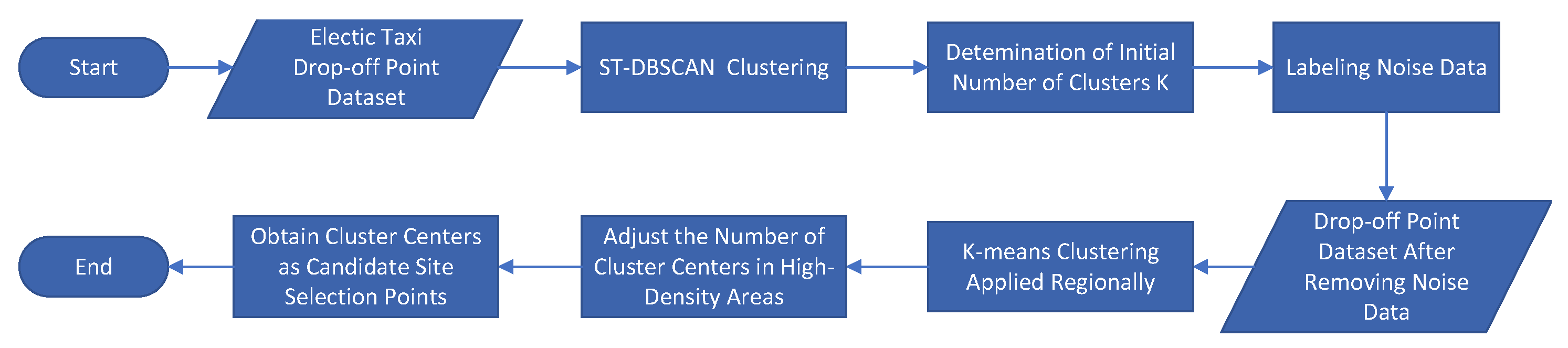
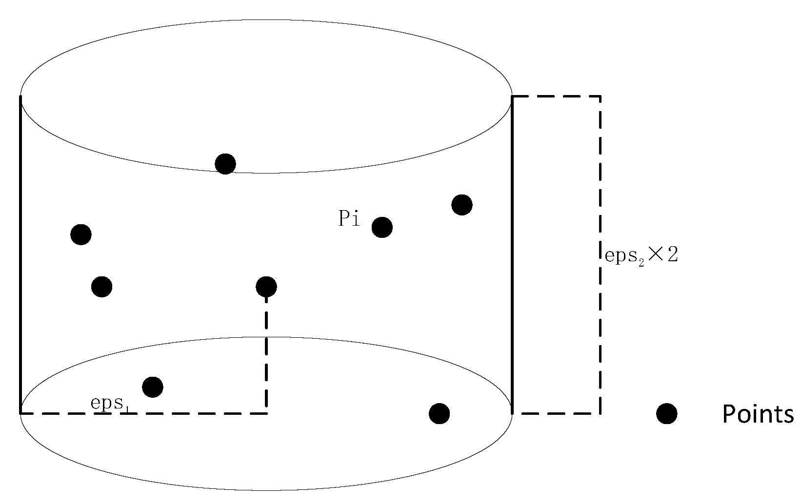
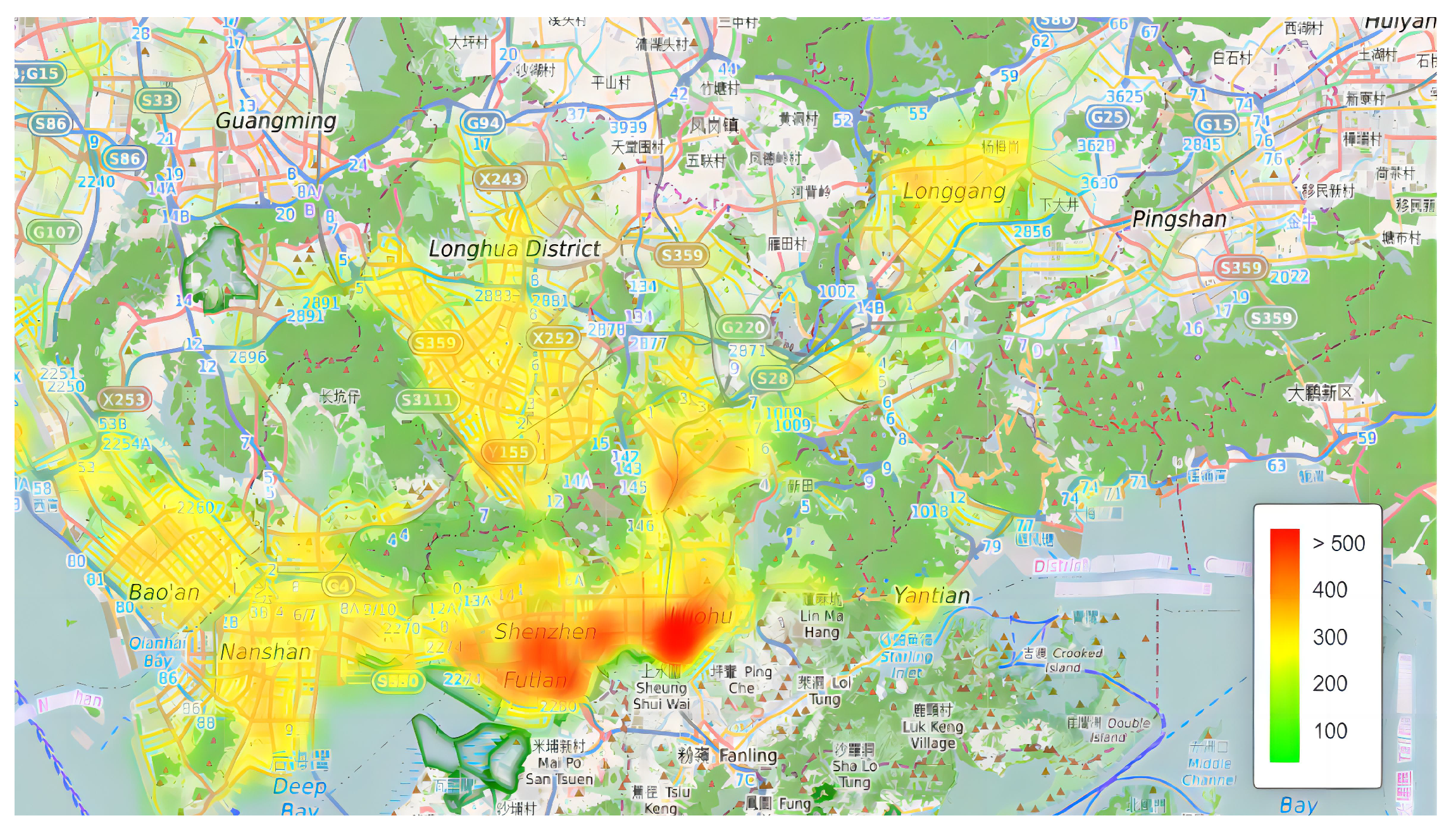
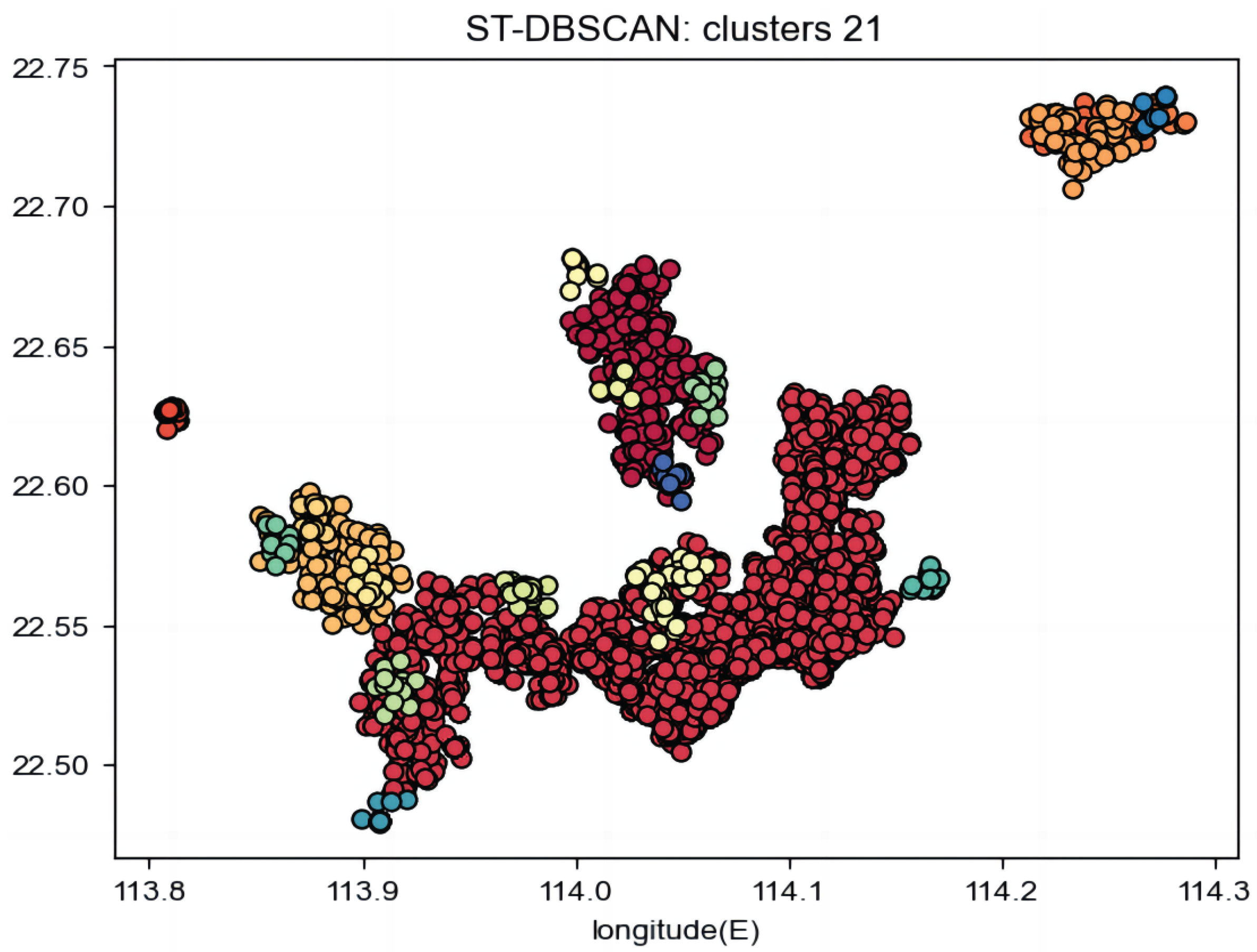


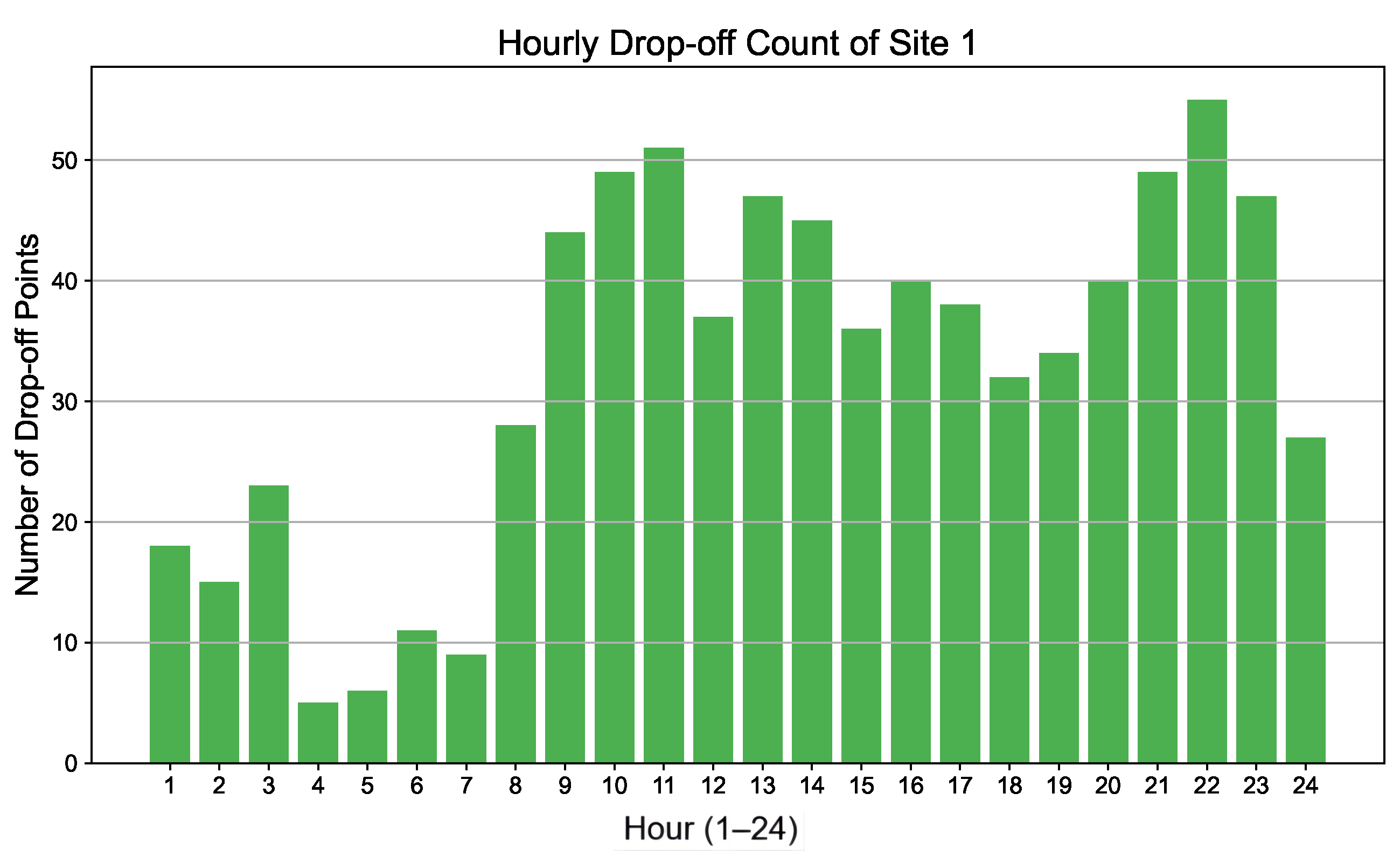
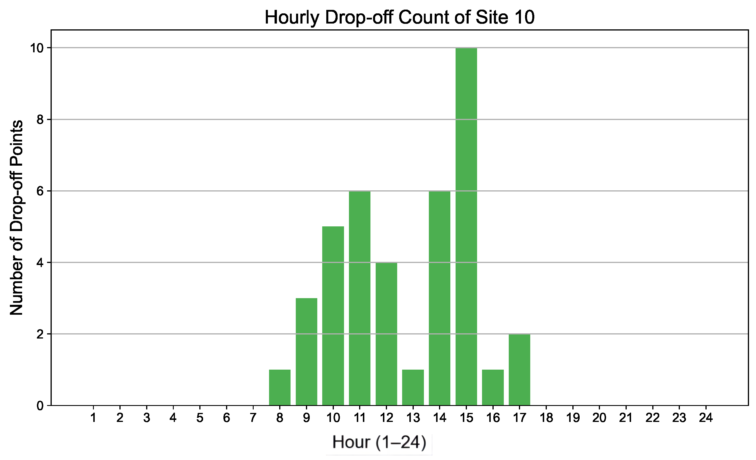
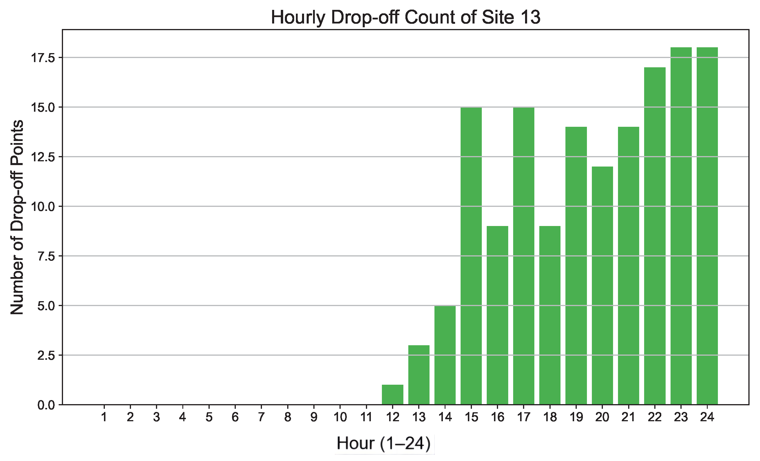
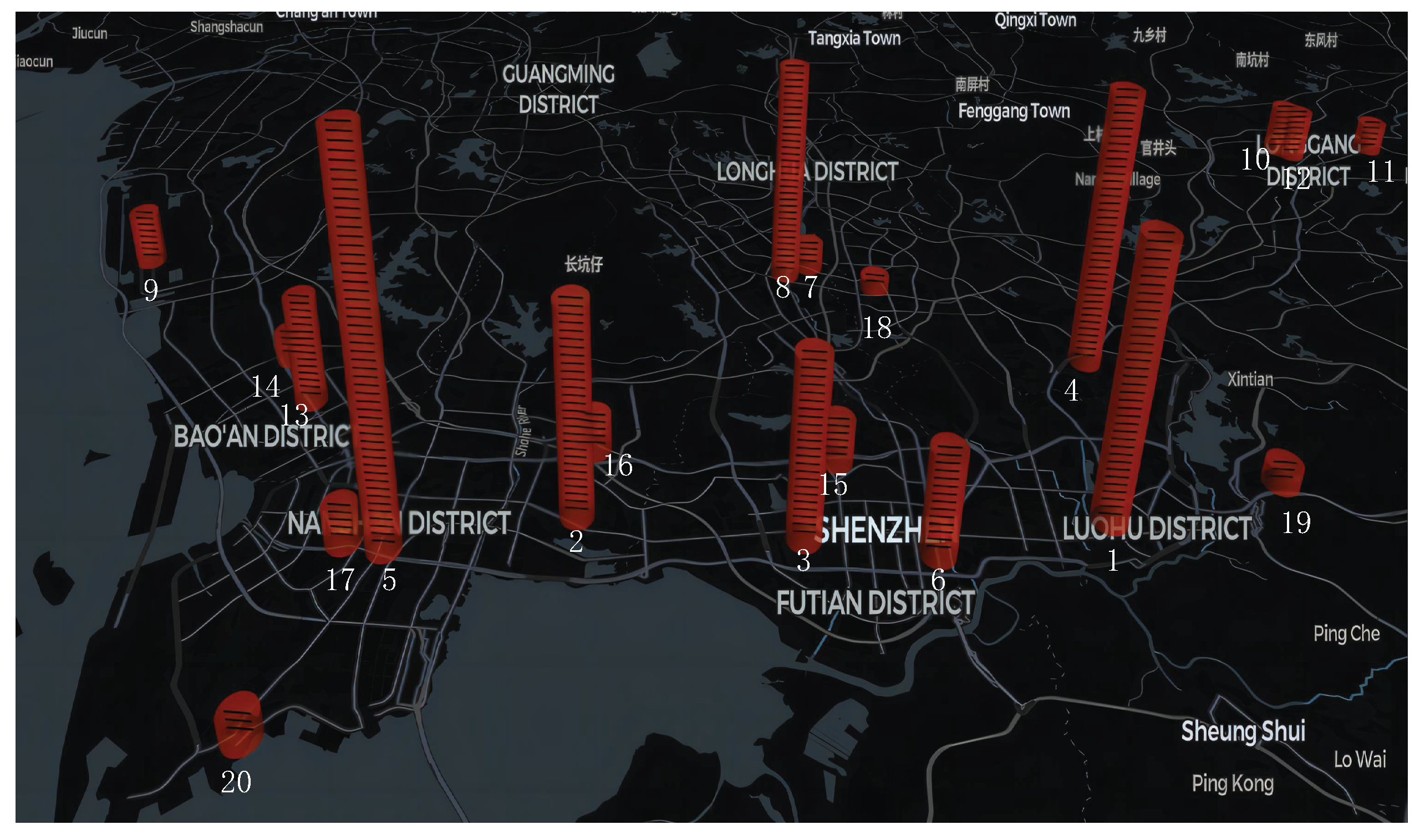
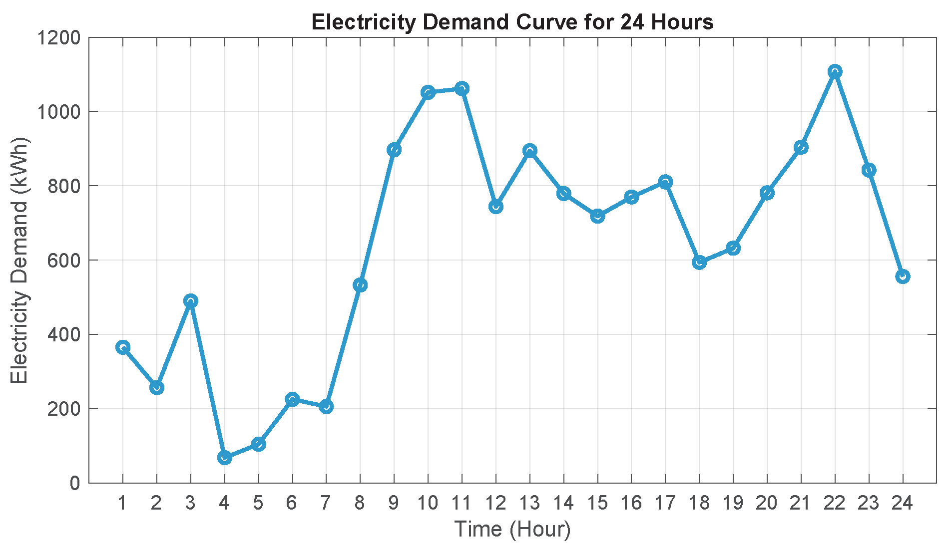
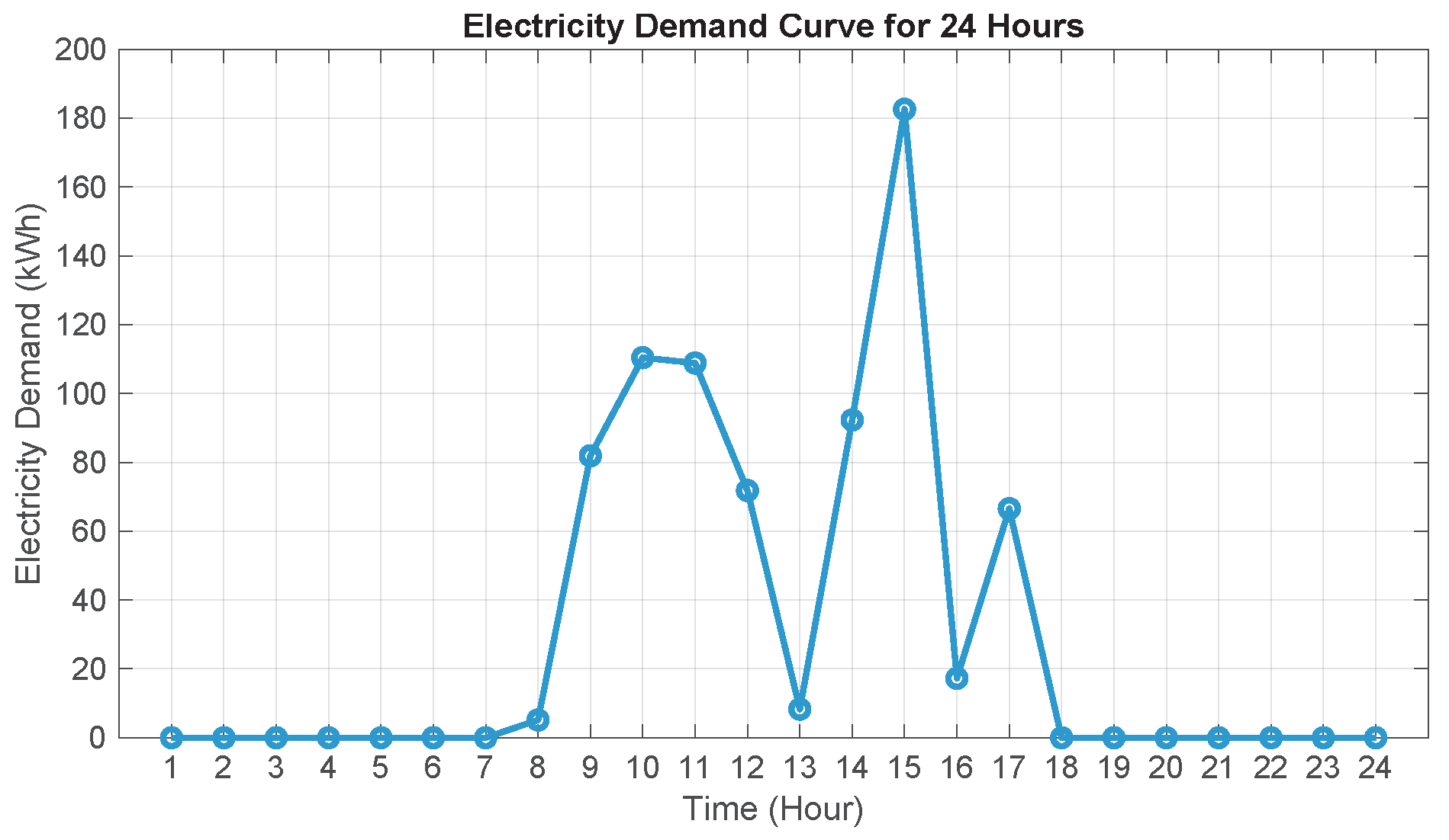
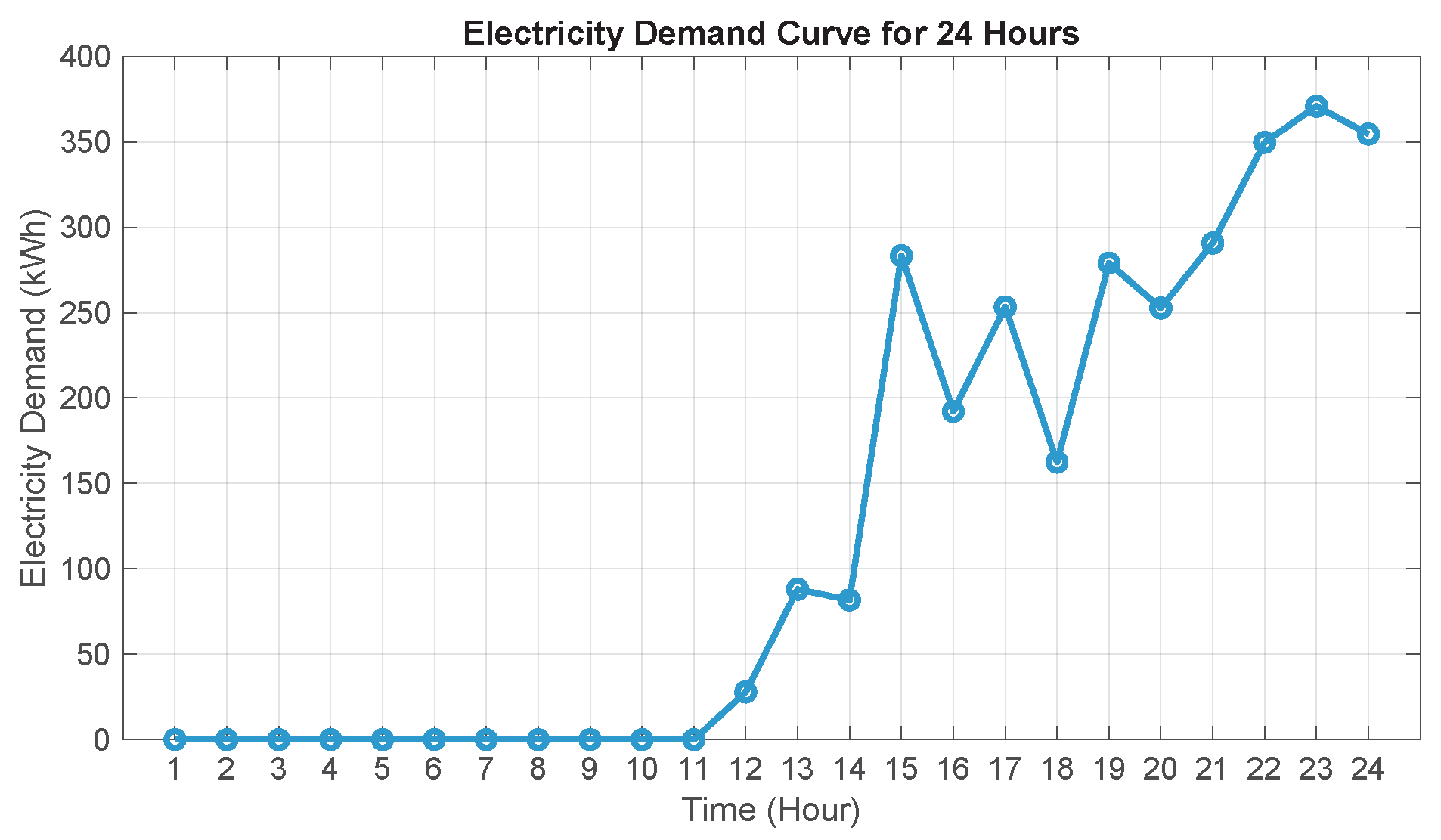
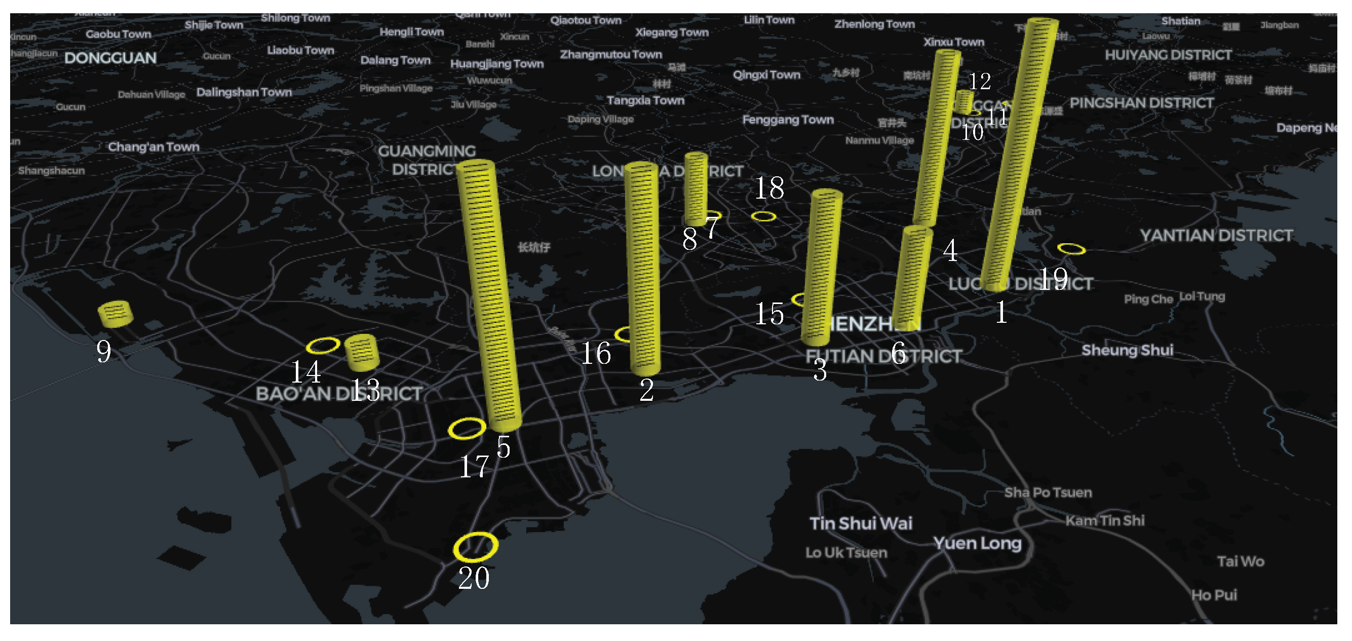
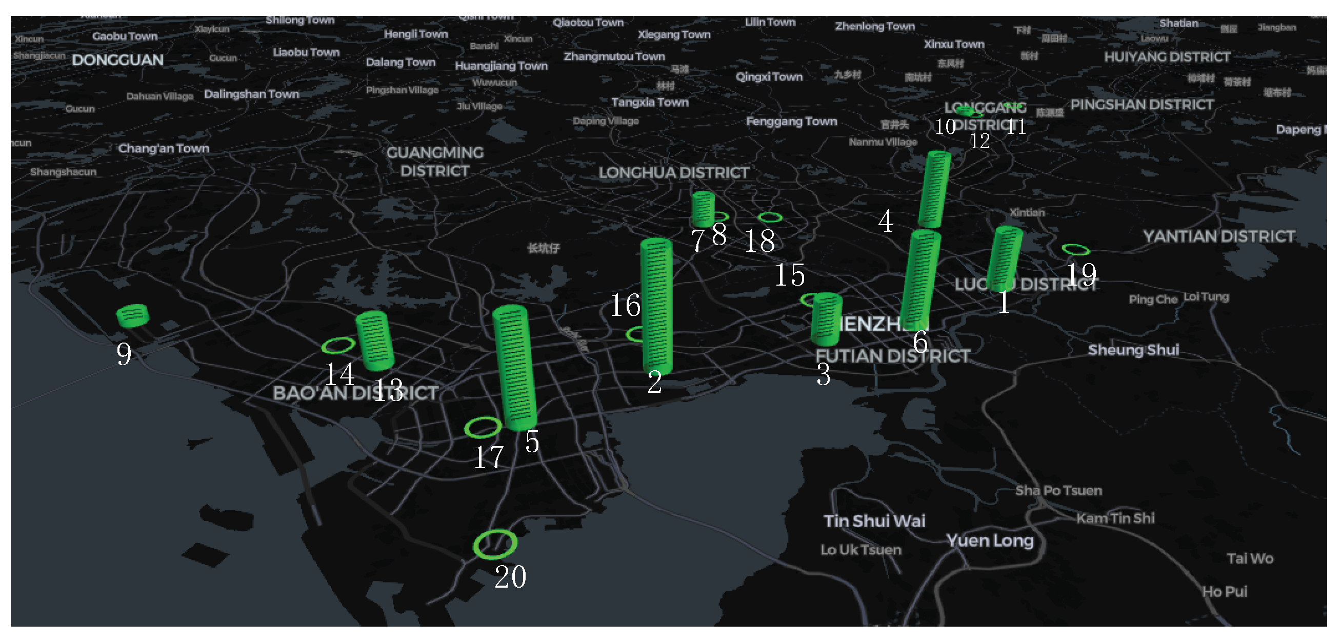

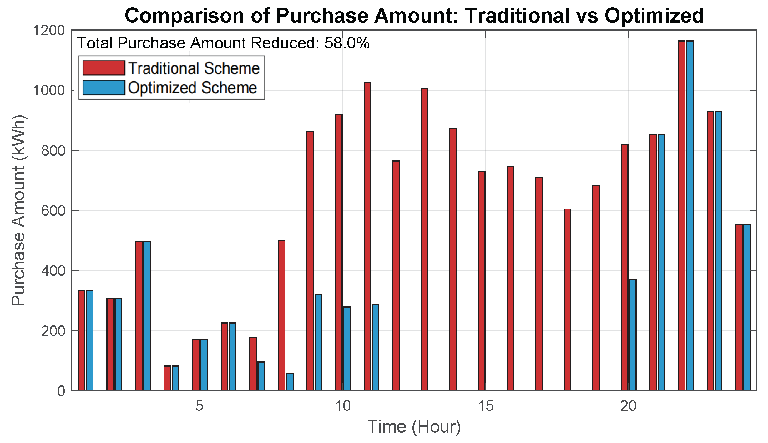
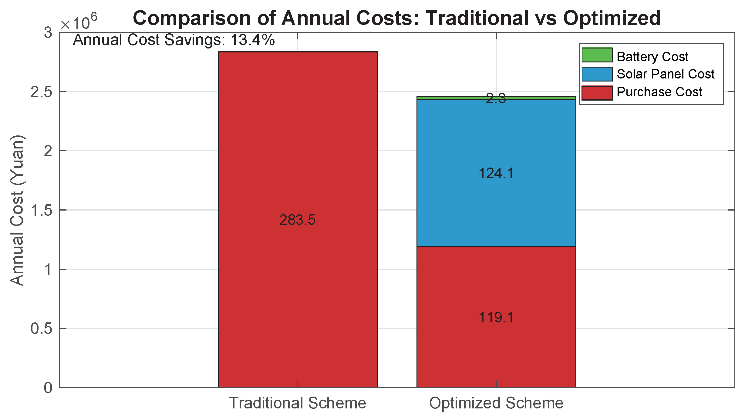
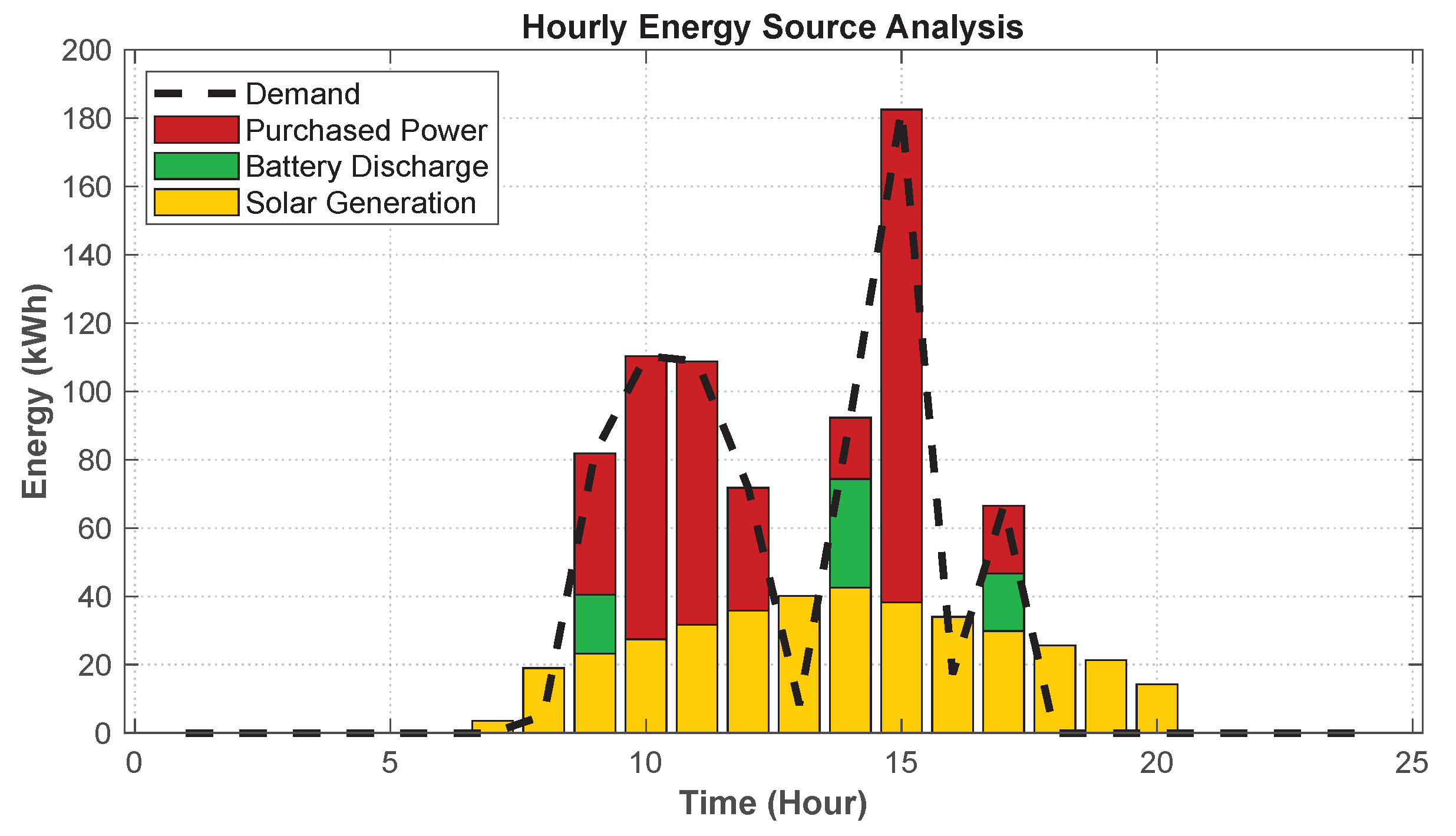
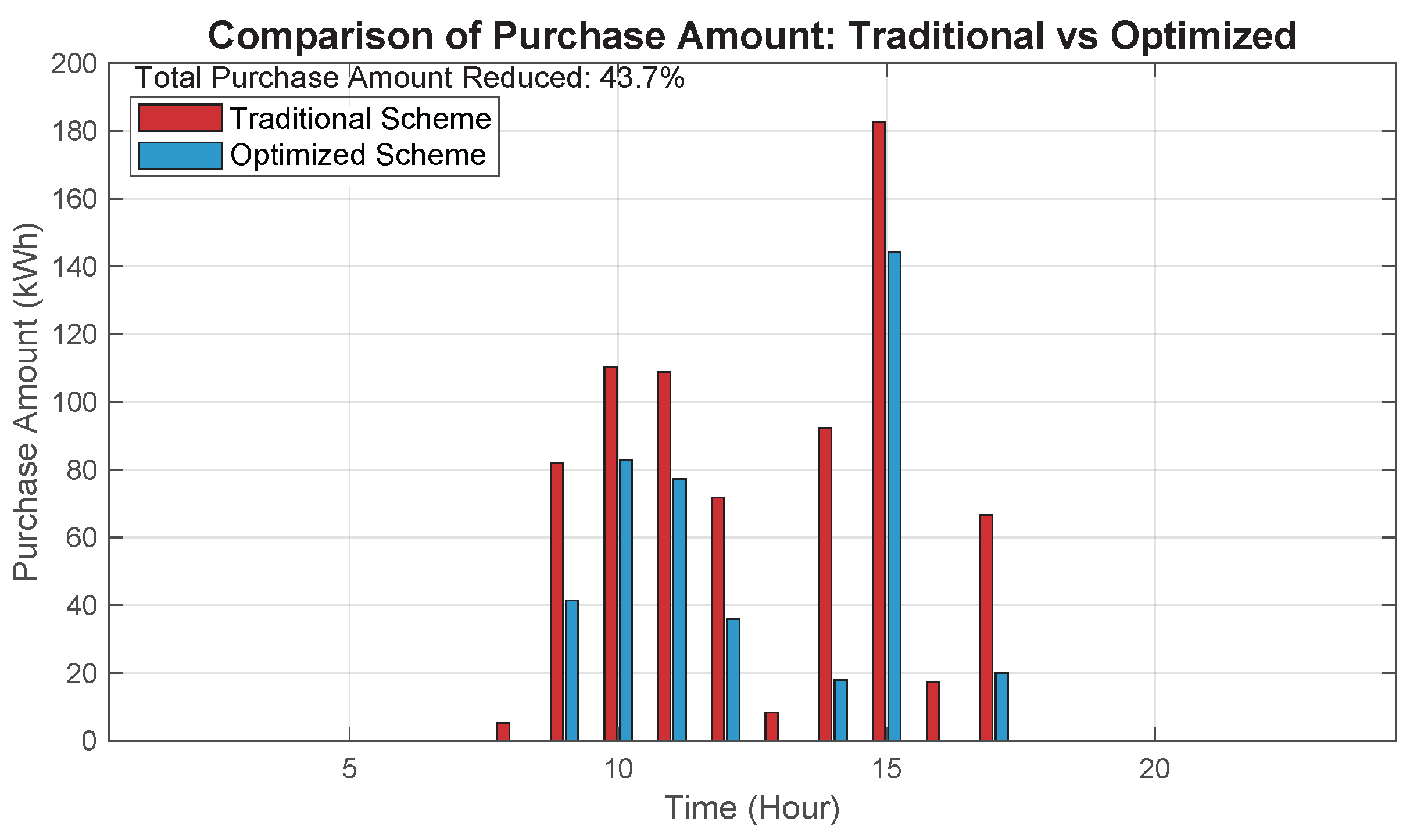
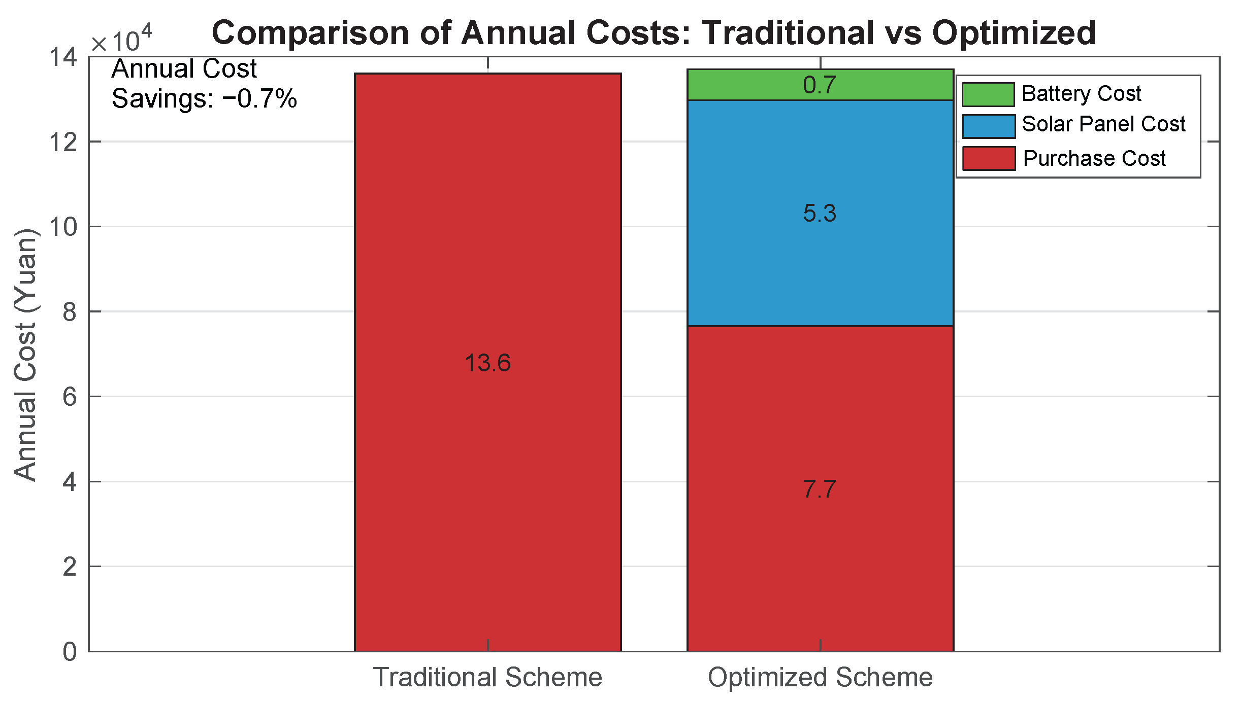
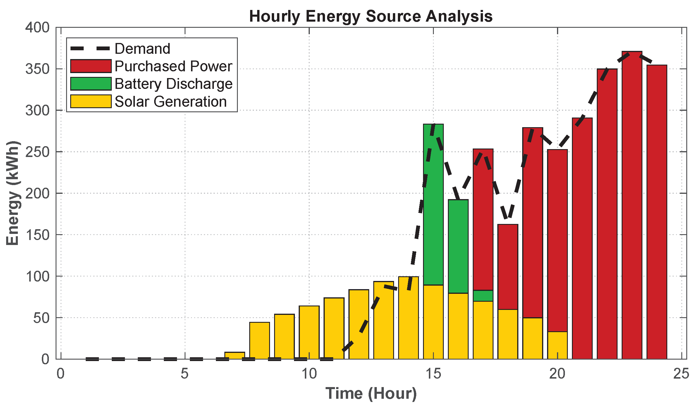
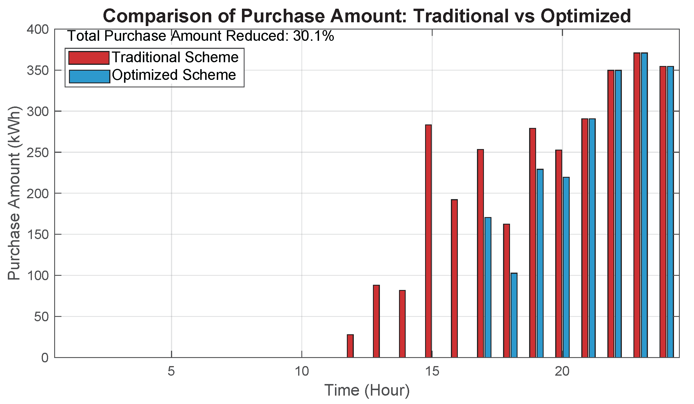
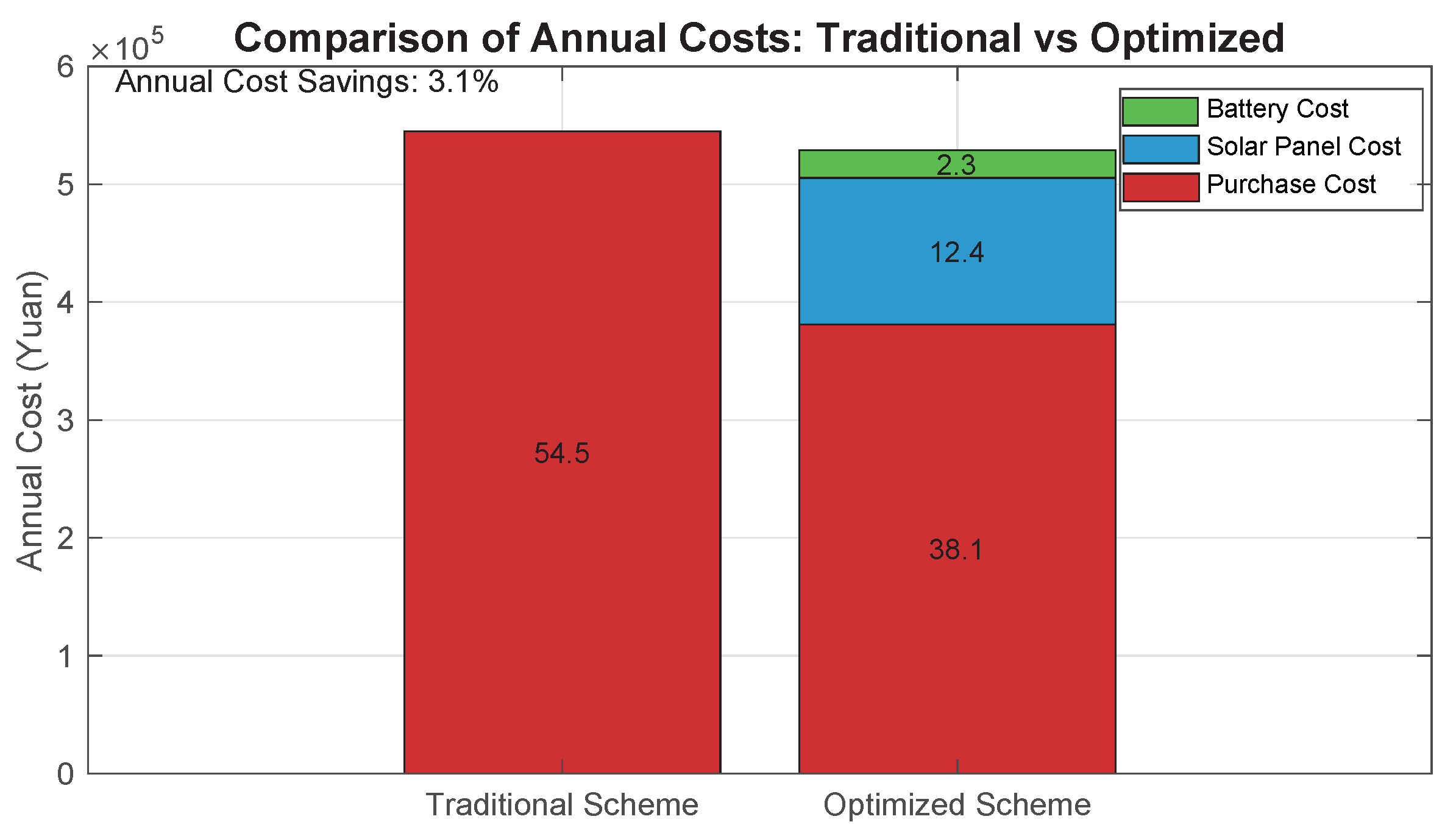
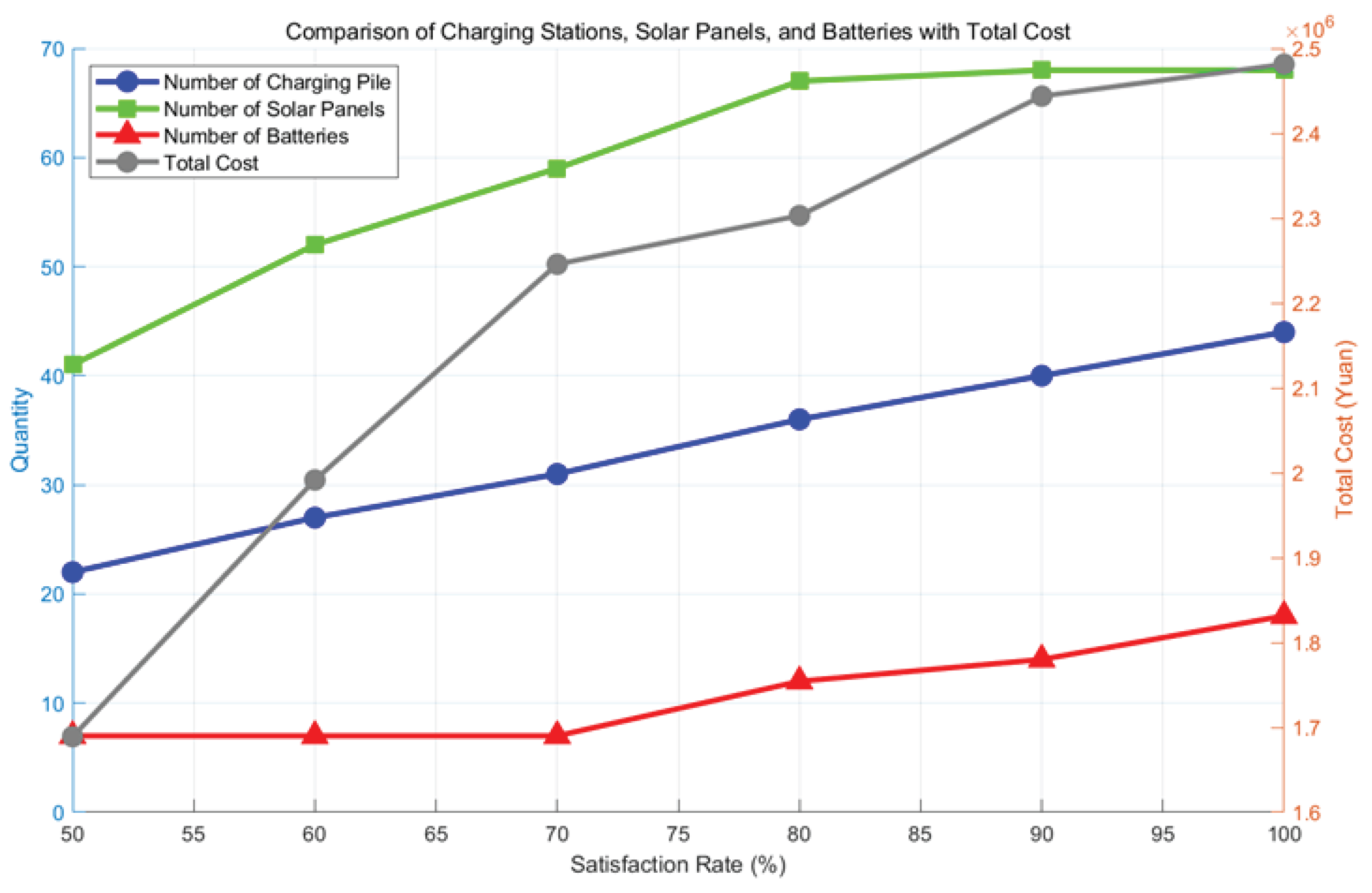

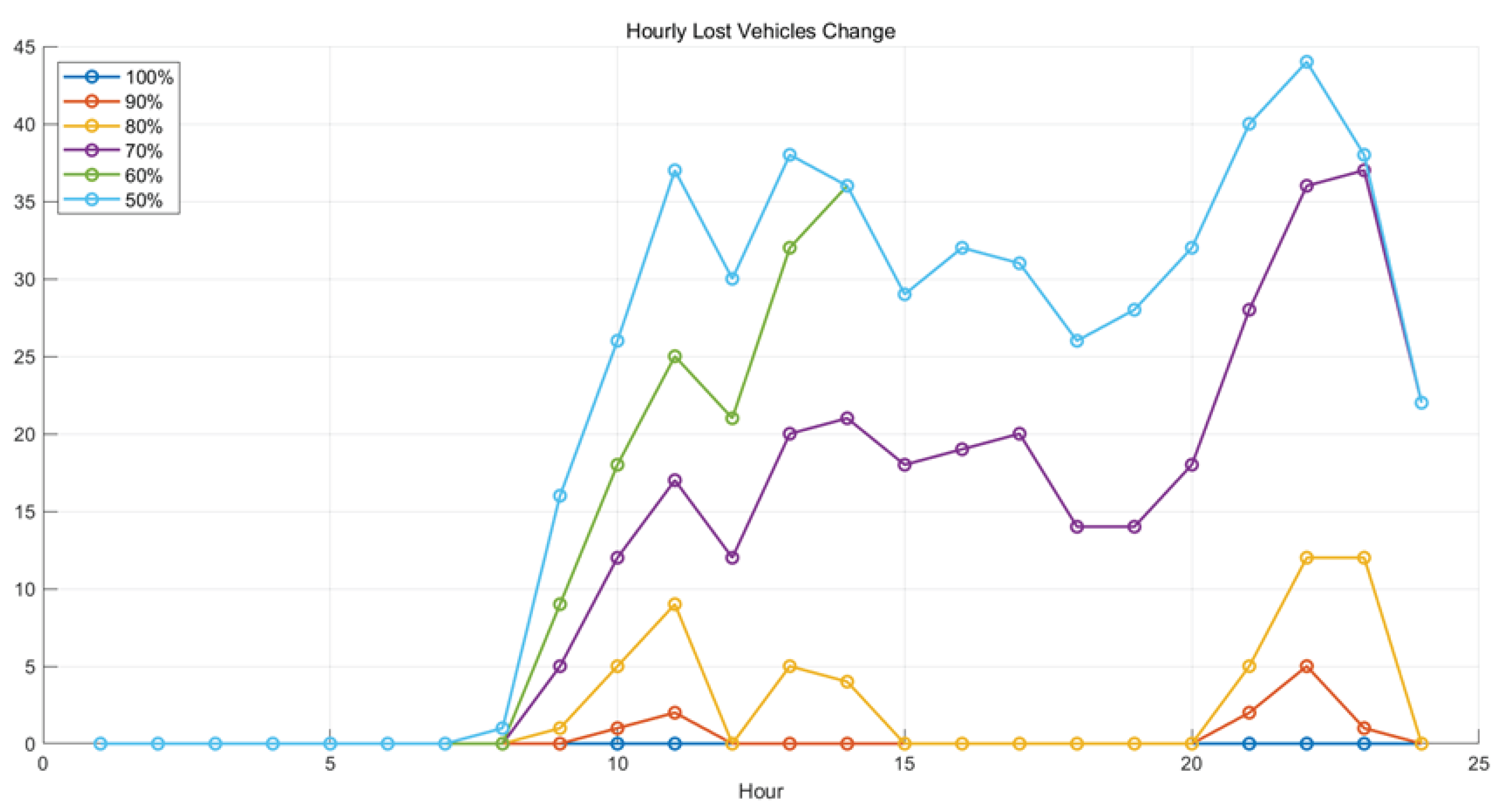
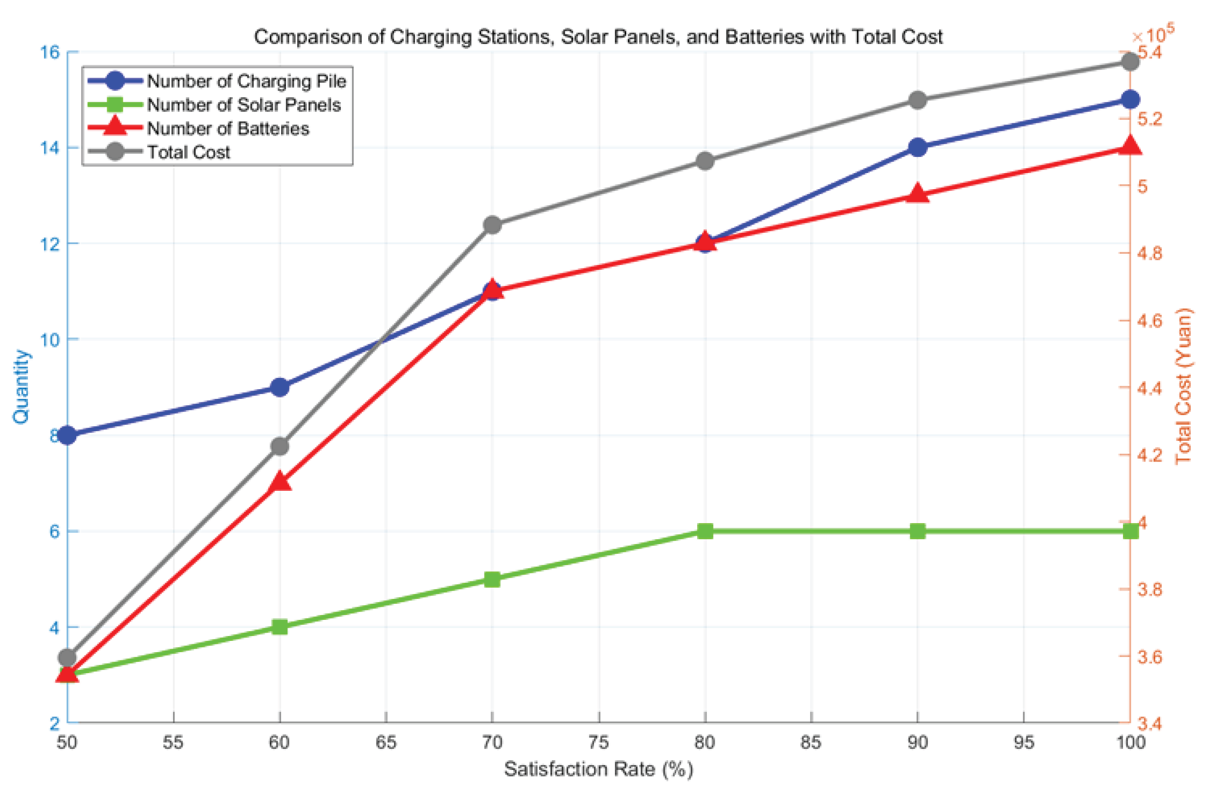
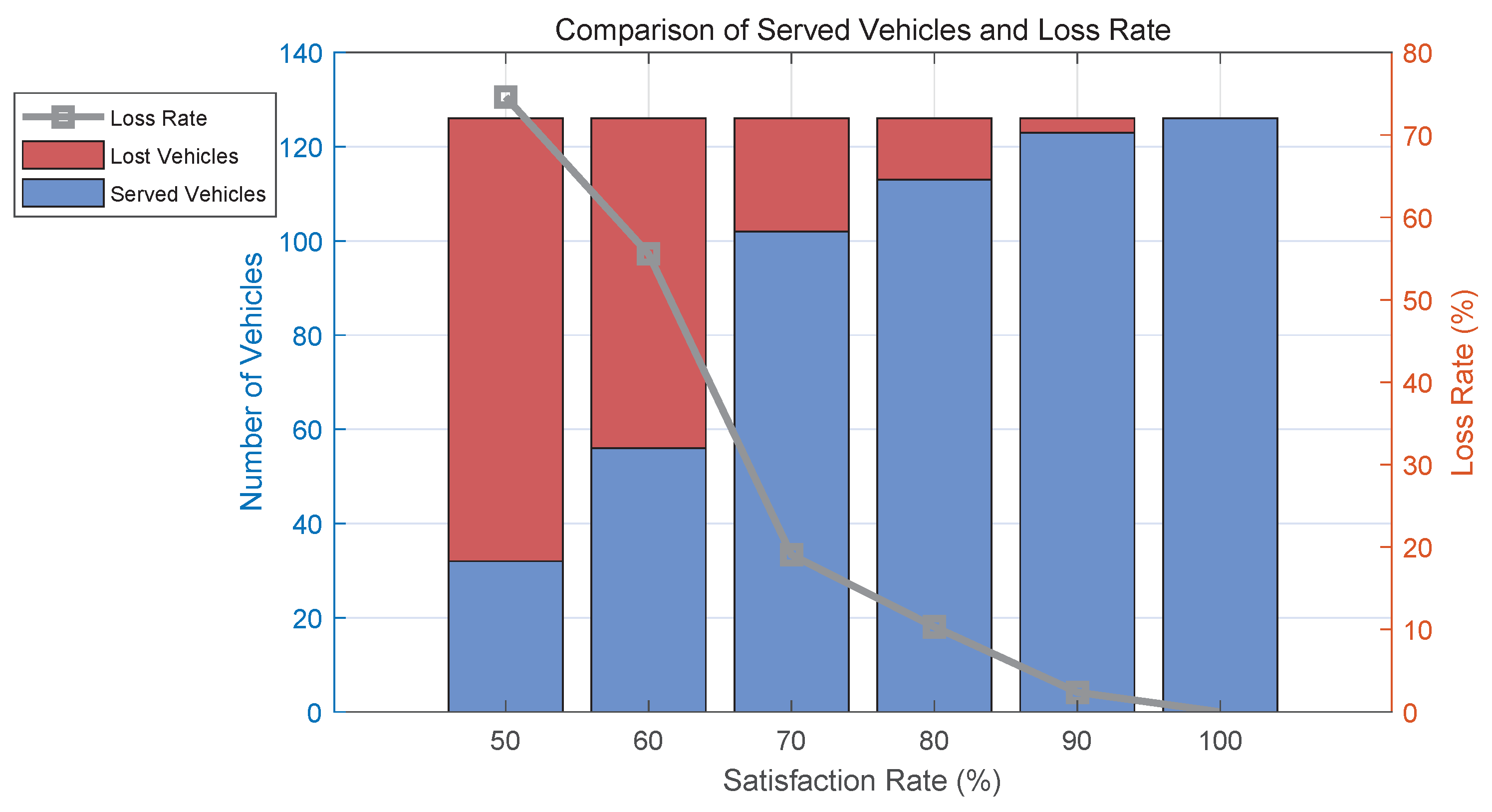
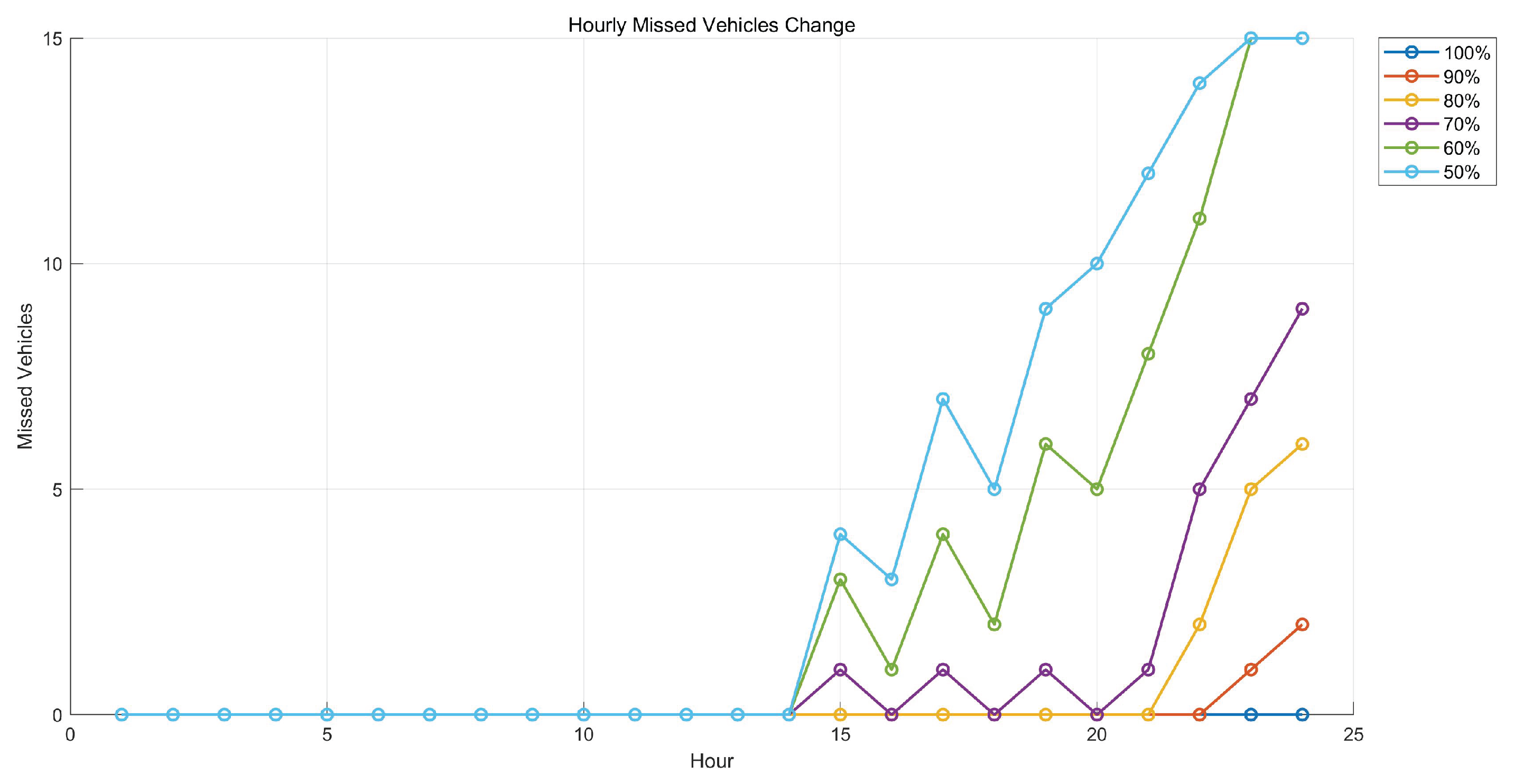
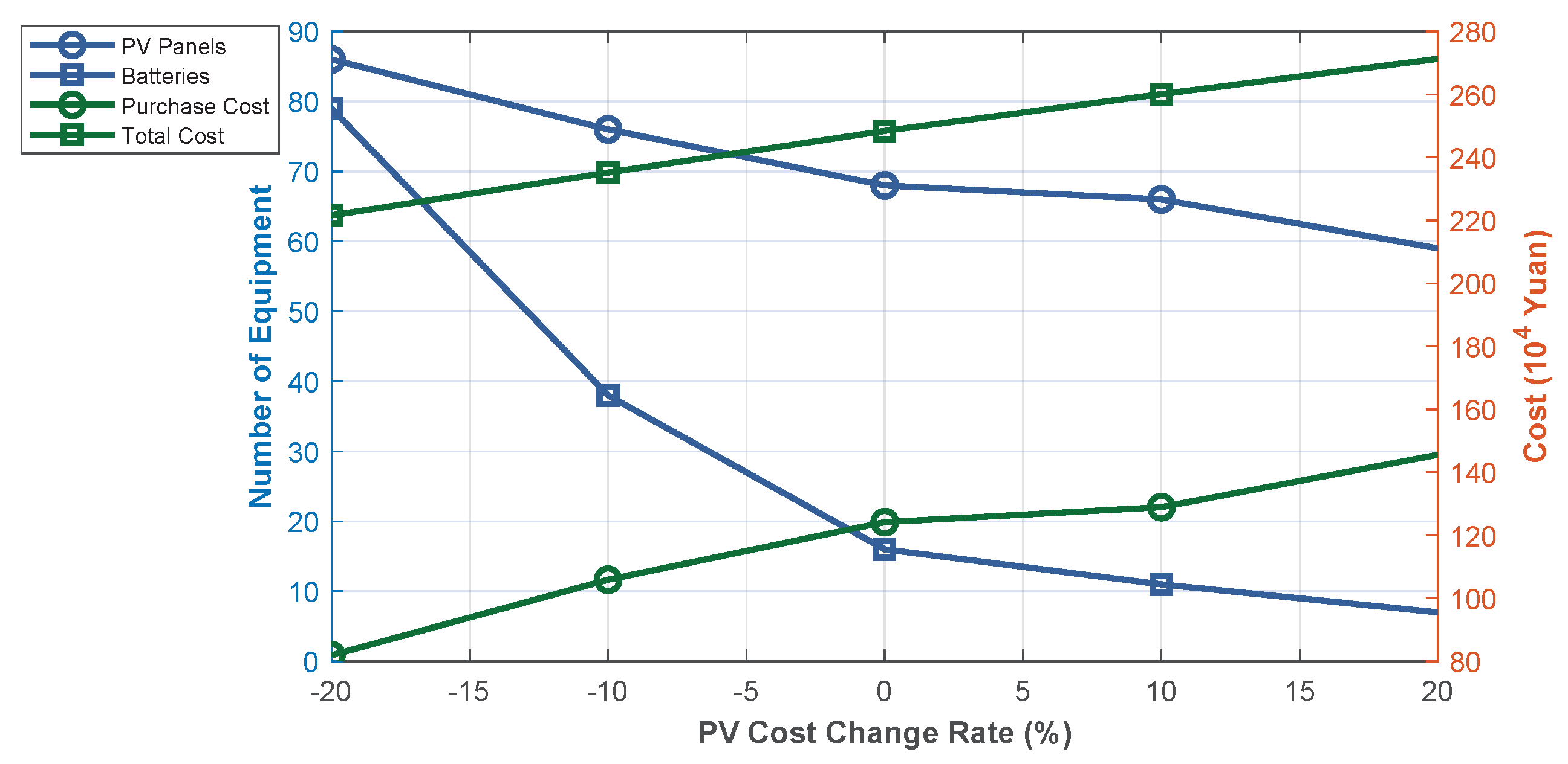
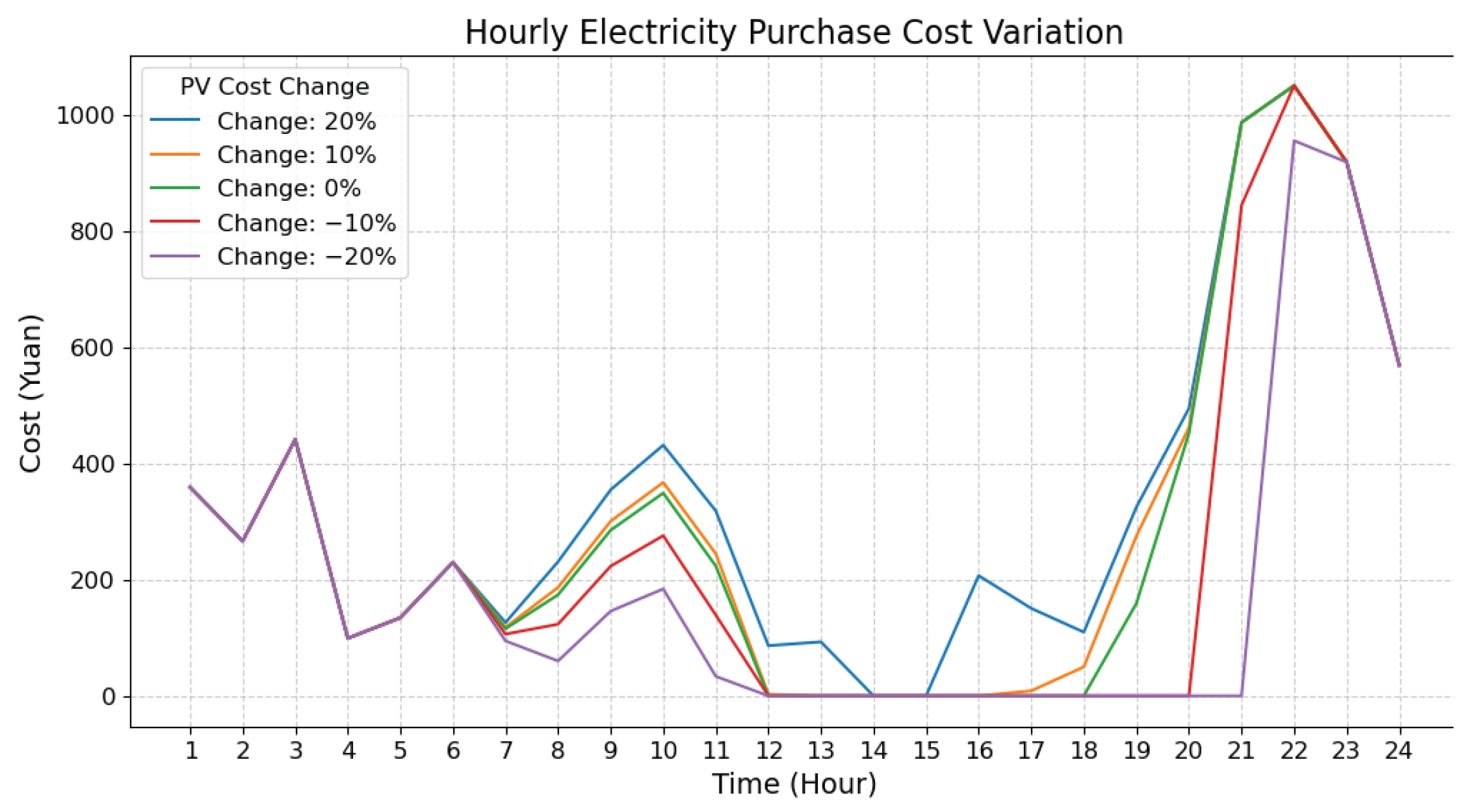
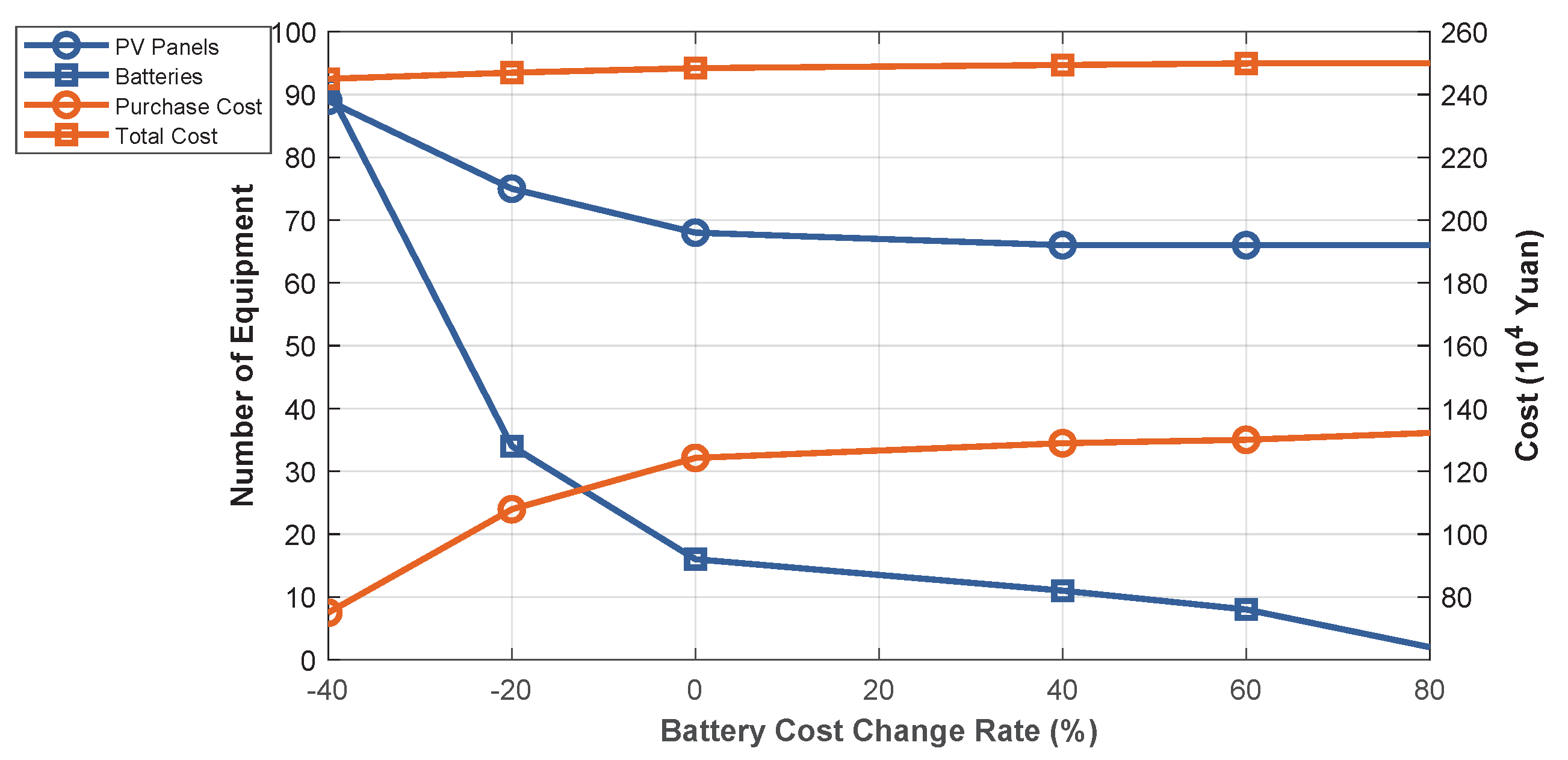
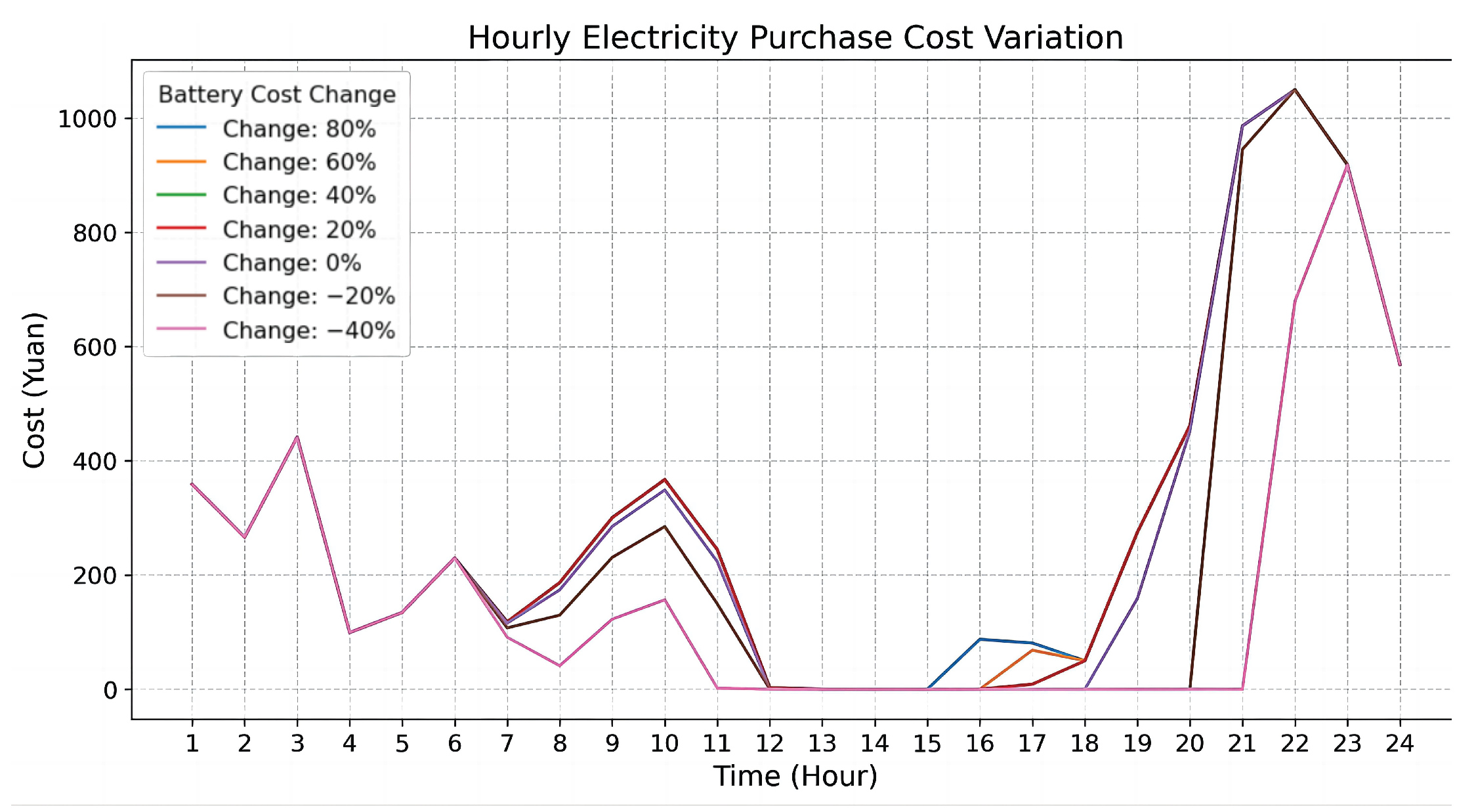
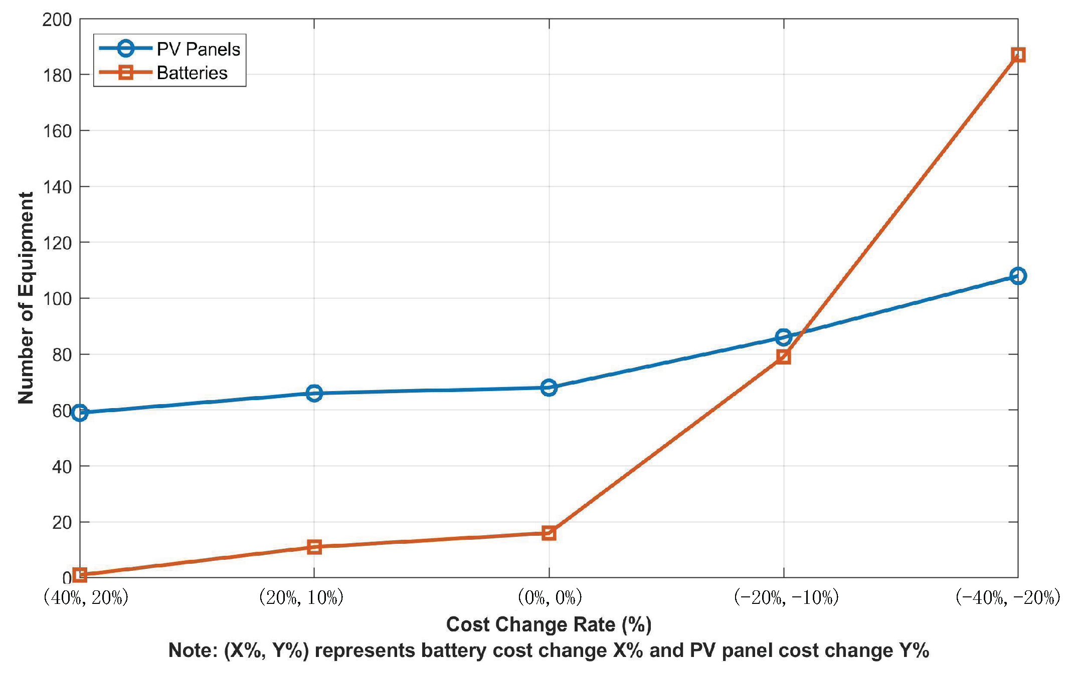
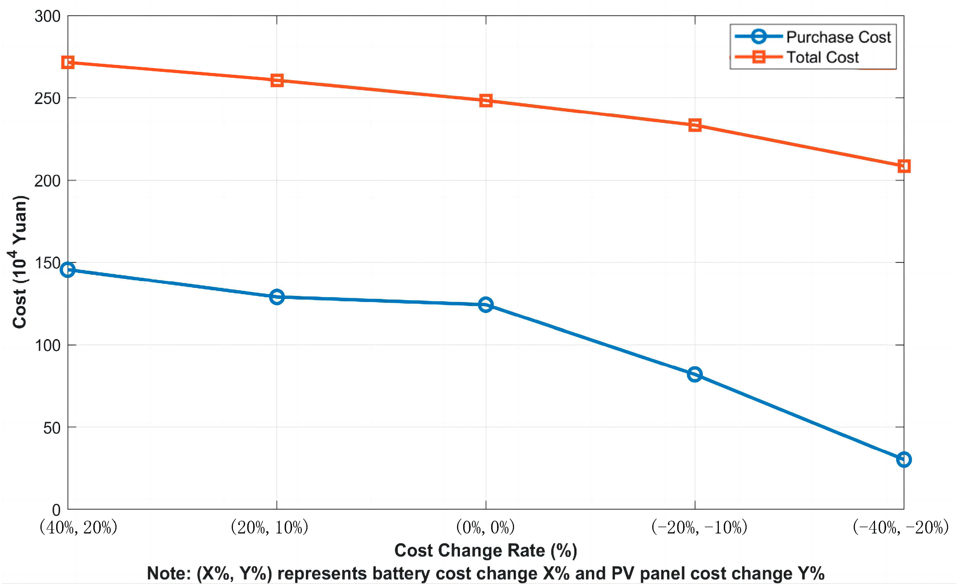
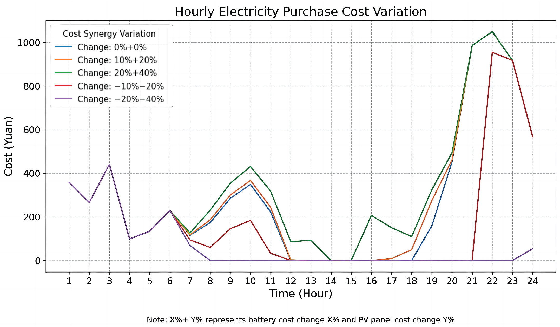
Disclaimer/Publisher’s Note: The statements, opinions and data contained in all publications are solely those of the individual author(s) and contributor(s) and not of MDPI and/or the editor(s). MDPI and/or the editor(s) disclaim responsibility for any injury to people or property resulting from any ideas, methods, instructions or products referred to in the content. |
© 2025 by the authors. Licensee MDPI, Basel, Switzerland. This article is an open access article distributed under the terms and conditions of the Creative Commons Attribution (CC BY) license (https://creativecommons.org/licenses/by/4.0/).