Abstract
This study explores the relationship between renewable and non-renewable energy consumption, economic growth (EG), and ecological footprint (EF) in Poland’s top 18 energy-importing countries from 2000 to 2022. While the energy-growth-environment nexus is well-studied, limited attention has been paid to how a single major energy-exporting country influences sustainability in its trade partners, a gap this study aims to fill. A panel dataset was constructed using five key variables: real GDP per capita, Poland’s fuel exports, ecological footprint per capita, renewable energy consumption, and primary energy consumption per capita. Methodologically, the study employs panel cointegration techniques, including FMOL and DOLS estimators for long-run analysis, as well as the VECM and Granger causality tests for the short run. The study’s main contribution lies in its novel focus on Poland’s export influence and the application of advanced econometric models to examine long-run and short-run effects. Results indicate a stable long-run cointegration relationship. Specifically, a 1% increase in renewable energy use is associated with a 0.0219% rise in GDP per capita. Additionally, Poland’s fuel exports and ecological footprint positively impact growth, whereas primary energy use is statistically insignificant. These findings offer practical implications for policymakers in Poland and its trading partners aiming to align energy trade with sustainability goals.
1. Introduction
The relationship between energy consumption (EC), economic growth (EG), and environmental degradation (ED) has been one of the most widely studied topics in sustainable development literature over the past four decades. This interest arises from growing concerns about climate change and environmental pollution, which are pressing for global challenges that require immediate and coordinated policy responses. The increasing reliance on fossil fuels is widely recognized as a primary driver of climate change. According to the Intergovernmental Panel on Climate Change (IPCC), human activities have already contributed to a global temperature increase of 1 °C above pre-industrial levels, with projections indicating a potential rise of up to 1.5 °C between 2030 and 2052 [1]. Achieving environmental stability, economic prosperity, and energy security is critical for the attainment of the Sustainable Development Goals (SDGs), especially in Europe, where there is a strong emphasis on access to sustainable and affordable energy. While energy plays a pivotal role in fostering economic development, its consumption, particularly from fossil fuel sources, has significant adverse effects on environmental quality. The combustion of fossil fuels increases greenhouse gas (GHG) emissions, contributing to air pollution and expanding both carbon and ecological footprints [2,3].
Numerous empirical studies have confirmed the strong link between fossil fuel consumption—particularly coal, oil, and natural gas—and environmental degradation across diverse contexts [4,5,6,7,8,9,10,11,12,13,14]. In response to these challenges, many countries are shifting toward renewable energy sources such as solar, wind, bioenergy, geothermal, and hydropower. These low-carbon alternatives are considered essential for mitigating environmental degradation while sustaining energy needs [15,16,17]. Unlike fossil fuels, renewable sources can produce electricity without emitting harmful GHGs [18]. However, some studies suggest that, under certain conditions, the adoption of renewables may not always lead to environmental improvement and could even exacerbate degradation in specific contexts [19,20].
Energy efficiency strategies have also emerged as viable tools to reduce energy consumption and its environmental consequences. Although these strategies can alleviate ecological damage to some extent, their benefits are often limited unless accompanied by broader systemic changes. Thus, transitioning to green energy and implementing comprehensive environmental regulations are critical. Strict environmental policies can enhance energy efficiency, reduce fossil fuel usage [21,22], encourage green energy production and consumption, and mitigate the negative environmental externalities of economic growth [23]. On the other hand, relaxed environmental regulations may have the opposite effect. Countries with lenient environmental standards risk becoming pollution havens, attracting environmentally damaging technologies and foreign investments in energy-intensive industries [24]. Such regulatory weaknesses often promote pollution-intensive industrial activities [25] and result in the net import of carbon-intensive goods in global trade dynamics, particularly when trading with countries that maintain stricter environmental laws.
In the broader literature, the relationship between EC and EG is generally discussed through four main hypotheses: growth, conservation, feedback, and neutrality. While many studies confirm a strong link between fossil fuel consumption and economic growth, the dynamics vary significantly across countries depending on income levels and energy sources. For instance, Yaşar [26] finds that in upper-middle and high-income countries, energy consumption and economic growth mutually reinforce each other in the long run, whereas the protection hypothesis holds for lower-middle-income countries. Similarly, Wolde-Rufael [27] reports a long-run relationship between electricity consumption and GDP in 17 African countries, with mixed directions of causality. In Vietnam, Tang et al. [28] observe a unidirectional causality from energy consumption to economic growth, arguing that policies promoting energy conservation may hinder growth. Studies in Algeria and MENA countries show a strong link between non-renewable energy consumption and economic growth, with Amri [29] emphasizing the dominant role of non-renewable sources in driving growth. Conversely, the impact of renewable energy consumption is more complex. For example, Yildirim et al. [30] find that waste-derived energy significantly influences GDP growth in the U.S., while other renewable sources do not, suggesting waste-derived energy as a key component for economic development. In European contexts, renewable energy consumption positively affects economic growth in Romania, as shown by Pirlogea and Cicea [31], whereas in Spain, natural gas consumption primarily drives short-term growth. Moreover, global factors are found to predominantly shape the energy-GDP nexus in OECD countries as Belke et al. [32] highlight, while in African nations, both energy consumption and economic growth show a positive correlation, highlighting the need for policies that encourage energy use to foster growth [33]. Structural policies aimed at improving economic efficiency can also promote energy conservation without hindering growth, as shown in Greece [34].
Building on this diverse empirical evidence, the present study seeks to deepen understanding of how renewable and non-renewable energy consumption differently affect economic growth and environmental outcomes in countries dependent on Poland’s energy exports. This nuanced perspective is essential for formulating targeted policy interventions in the context of sustainable development. The role of energy in the EKC framework is indispensable, as energy consumption is closely linked to both economic activity and environmental outcomes. Recently, the ecological footprint (EF) has become a widely adopted indicator of environmental quality and sustainability. The EF measures the biologically productive land and water area required to produce the resources consumed by a population and absorb the associated waste, using current technology. It is expressed in global hectares (gha) and reflects both the pressure placed on the environment and the sustainability of resources us [35]. Since the articulation of the sustainability concept in the Brundtland Report [36] and subsequent global initiatives aimed at sustainable development [37], the EF has gained relevance as a comprehensive measure of environmental stress. Ideally, humanity’s EF should not exceed 1.7 gha per person—the planet’s available bio-capacity. However, since 1971, the world has entered an ecological deficit, with 2018 figures indicating an EF of 2.77 gha per capita and a per capita bio-capacity of just 1.58 gha [38]. This widening gap underscores the persistent global failure to achieve sustainable development, despite decades of international commitment. These values are, however, heterogeneous across regions and within countries. The global depletion of fossil fuel reserves and the resultant increase in EF have intensified the search for alternative, environmentally benign energy sources. Renewable energy has thus been promoted not only for its low environmental impact but also for its role in reducing energy import dependence, improving trade balances, lowering production costs, and fostering green production practices. According to the International Energy Agency [39], global renewable energy capacity is expected to increase by 2.7 times by 2030, surpassing current national targets by nearly 25%, though still falling short of the COP28 objective of tripling capacity. This anticipated expansion is driven by falling technology costs, improved permitting frameworks, supportive government policies in over 140 countries, and increased investment in domestic solar and wind manufacturing. The European Union has played a leading role in this transition, achieving 22.1% of its energy consumption from renewables by 2020, surpassing its 20% target, a remarkable increase from 9.6% in 2004 [40]. However, significant disparities persist across member states, with Sweden leading at 60%, and Malta and Luxembourg trailing below 13%. The 2022 Russian invasion of Ukraine further accelerated Europe’s energy diversification agenda, reinforcing the strategic importance of renewables in ensuring energy security. Despite this momentum, the global energy sector continues to face challenges, particularly with respect to scaling technologies like hydrogen, as well as insufficient policy support in some regions [41].
Renewable energy consumption has seen significant growth across the electricity, transport, and heating sectors. Projections indicate that by 2030, renewables will constitute 46% of global electricity generation, predominantly driven by wind and solar sources. While traditional biofuels dominate the transport sector, renewable electricity and hydrogen fuels are increasingly important, particularly in road and aviation. In the heating sector, technologies such as solar thermal, heat pumps, and geothermal systems are contributing to fossil fuel substitution despite macroeconomic challenges such as inflation and high interest rates. Nonetheless, policy uncertainty, financial barriers, and market integration issues continue to impede the full-scale adoption of renewable energy technologies. Meeting the Net Zero by 2050 goals will require accelerated technological innovation and enhanced policy alignment. Given this context, the present study offers several critical contributions. First, it investigates the differential impacts of renewable versus non-renewable energy consumption on economic growth and environmental sustainability using a nuanced methodological approach. However, what distinguishes this contribution is not only the methodological rigor but also the recognition that renewable and non-renewable sources may influence economic and environmental outcomes in fundamentally different ways, a dimension often overlooked in prior studies. Second, unlike prior studies focused on energy-importing countries from Russia [42], this study uniquely focuses on countries that receive a significant share of Poland’s energy exports. Third, the study integrates the energy consumption–economic growth–environmental degradation (EC–EG–ED) nexus within a unified empirical framework and applies it, for the first time, to this specific regional context. This approach provides a comprehensive perspective on the interconnected nature of energy, economy, and environment.
Fourth, it employs the ecological footprint (EF) as the proxy for environmental degradation, a more holistic metric encompassing human impacts on land, water, and air [13]. To analyze the dynamic interrelationships among these variables, this study utilizes the Panel Vector Autoregression (PVAR) model. In line with the methodological framework and research objectives, this study tests the following central hypotheses:
H1.
An energy supply shock originating from Poland adversely affects the economic growth trajectories of the dependent countries while simultaneously exacerbating their ecological footprints.
H2.
Substituting imported fossil-based energy with domestic renewable sources facilitates economic growth without intensifying environmental degradation. Ultimately, this study aims to propose empirically grounded policy recommendations for nations dependent on Poland energy exports. These recommendations are designed to support a transition toward cleaner energy systems while safeguarding economic development and ecological integrity.
2. Materials and Methods
2.1. Panel Vector Auto Regression
The Panel Vector Autoregression (PVAR) methodology has several practical advantages that make it more appropriate for analyzing macroeconomic dynamics. First, the statistical model of PVAR is neutral concerning a certain theory of growth or development and is more based on the current movements of a series than on a specific notion of macroeconomics, which, if disapproved, can be misleading [43]. Second, the current PVAR model does not distinguish between endogenous and exogenous variables; rather, all variables are viewed as mutually endogenous, keeping with the interdependent facts. Each PVAR variable depends on additional variables in addition to its historical manifestation, demonstrating a true simultaneity between the variables and their treatment. Third, for small open economies, where endogenous and exogenous shocks are the most significant causes of macroeconomic dynamics, PVAR offers a model for these types of shocks. Additionally, PVAR is quite simple for efficient and coherent estimations in both cases: a single nation or a panel of other countries. As a crucial instrument for examining the connection between ecological footprint, economic growth, FDI, and PS PVAR also provides a reasonable estimate. The linear equation of a P-order, k-variable PVAR model shown in the form of a panel-specific fixed effect can be represented as follows.
In the equation, yit is the (1xk) vector of dependent variables, xit is the (1xk) vector of exogenous variables, and uit and eit are (1xk) dimensional, constant effects, and idiosyncratic error terms vectors. With A1, A2,…, Ap−1, Ap, shown in the equation, the (1xk) dimensional B matrix is estimated. Extending the traditional vector autoregressive model to panel data settings, the panel vector autoregression (PVAR) framework allows modeling interdependencies between multiple time series across cross-sectional units. To analyze long-run equilibria and short-term dynamics simultaneously, the panel vector error correction model (PVECM) is applied. This approach is valid when the variables are integrated of order one, I(1), and share one or more cointegrating relationships [43,44].
The existence of cointegration indicates a stable long-term association among the variables, while deviations from equilibrium are corrected over time via an error correction mechanism. This correction process adjusts the dependent variables according to both the equilibrium deviations and short-run fluctuations. Appropriate lag lengths for the model are determined using standard selection criteria [45].
The VECM model can be formally expressed as follows, illustrating how the error correction term and short-run dynamics are incorporated into the system.
Lag q denotes the chosen lag length, and Δ, represent the first difference operator. The model includes an error correction term. ℇ, which captures deviations from long-run equilibrium, and a stochastic disturbance term, u. Estimation of the VECM is performed using the seemingly unrelated regression (SUR) technique, allowing for correlations across cross-sectional units in both residuals and parameter vectors.
2.2. Panel Unit Root Test
Prior to applying the PVAR methodology, the initial step in the estimation process involves examining the stationarity properties of all variables in the dataset. Panel unit root tests are generally categorized into two types: first-generation tests, which assume cross-sectional independence, and second-generation tests, which allow for cross-sectional dependence among units [46]. Examples of first-generation panel unit root tests include those developed by Levin et al. [47], Im et al. [48], Maddala and Wu [49], and Hadri [50].
Whereas the second generation contains Pesaran [51], Moon and Peroon [52], Smith et al. [53], and Carrion-I-Silvestre et al. [54]. However, if significant levels of positive residual cross-section dependence exist and if it is not considered, Panel unit root tests of the first generation may result in inaccurate results because of the presence of size distortions [55]. Therefore, it is vital to examine cross-sectional dependence to select the most suitable estimator in panel data analysis. To test for this dependence, the diagnostic approach introduced by Pesaran [56] was applied. Furthermore, tests developed by Salim and Rafiq [57], Breusch and Pagan [58], the LM test, Pesaran’s CD test [58], as well as Baltagi et al.’s bias-corrected CD test [59], serve to identify cross-sectional dependence effectively.
2.3. Panel Cointegration Tests
To assess whether non-stationary variables share a stable long-term equilibrium, panel cointegration tests are employed. The widespread availability of panel datasets has encouraged the advancement of various statistical techniques tailored for such data structures. Recent contributions in the literature have particularly emphasized methods that enable the detection of cointegration relationships within a panel context.
In this study, the following types of cointegration tests were used for the panels: Pedroni [60] and a Fisher-type test using the Johansen methodology.
2.4. Data
From an initial list of 24 countries representing Poland’s top fuel importers, this study focuses on 18 key partners to which Poland exports the majority of its fuel. The selection was based on the availability and consistency of data covering both the long-term period from 2000 to 2022 and the most recent year, 2022. This selection is based on both the most recent data for 2022 and the 2000–2022 period averages. Only countries that appear in both the long-term average and the 2022 data were considered for inclusion. As mentioned in the Table 1, countries such as Ireland, Egypt, China, Turkey and the United States were excluded due to their appearance in only one of the two periods. Furthermore, Hungary, Serbia, and Ukraine were excluded due to insufficient data for key variables. Thus, the final sample consists of 18 countries. Table 1 provides a comparative overview of these export destinations, detailing average export volumes and shares over the entire period alongside the data for 2022. The results indicate substantial shifts in Poland’s export distribution, with Ukraine emerging as the largest recipient in 2022, accounting for 21.45% of total fuel exports, followed by the Slovak Republic (15.47%), the Czech Republic (13.64%), and Austria (11.30%). This trend highlights significant changes in Poland’s trade dynamics, where certain countries have increased their export shares compared to historical averages.

Table 1.
Poland fuels exports by country (US$ Thousand).
The empirical analysis employs a panel dataset constructed from multiple international sources. Five variables are used to capture the central dimensions of the study: real GDP per capita, Poland’s fuel exports to individual countries, ecological footprint per capita, the share of renewable energy in total energy consumption, and primary energy consumption per capita. Among these, primary energy consumption per capita serves as the dependent variable, reflecting overall energy usage patterns within each country. The definitions of these variables, along with their corresponding data sources, are summarized in Table 2.
Table 2.
Variable Definitions and Data Sources.
Figure 1 presents the temporal variations of the key variables examined in this study, displaying their trends across the countries and years included in the dataset. The graphs offer a comprehensive visual representation of the development of each variable over the study period, highlighting the cross-country and temporal dynamics.
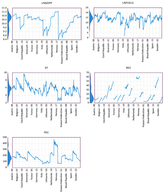
Figure 1.
Distribution and Temporal Trends of the Key Variables Across Countries.
2.5. Expected Empirical Outcomes of Hypotheses
To ensure clarity and reproducibility in hypothesis testing, we explicitly map the expected empirical outcomes for each hypothesis. For H1, a negative and statistically significant effect of fossil fuel shocks (proxied by LNFUELS) on GDP per capita (LNGDPP), along with a positive effect on ecological footprint (EF), would support the hypothesis that energy shocks originating from Poland hinder economic growth while exacerbating environmental degradation.
For H2, a positive coefficient of renewable energy consumption (REC) on LNGDPP, combined with a negative or insignificant impact on EF, would confirm that substituting fossil-based imports with domestic renewables fosters economic growth without intensifying environmental harm. These expectations serve as a benchmark for interpreting the results obtained from the VECM model as well as DOLS and FMOLS estimations.
3. Results
Descriptive measures and the correlation structure of the study variables are provided in Table 3. The Jarque–Bera test results indicate that none of the variables follow a normal distribution at the 5% significance level. Table 3 also summarizes the key patterns observed in the data. It shows that countries with higher levels of real GDP per capita (LNPGDP) also tend to have higher fuel export levels (LNFUELS), greater ecological footprints (EF), and higher levels of both renewable (REC) and primary energy consumption (PEC). This suggests that economic prosperity in the sample countries is closely linked with both traditional and modern energy consumption patterns. Notably, fuel exports show a positive relationship with primary energy use and environmental impact (EF), but a negative association with renewable energy share (REC), indicating that economies relying more on fuel exports may lag in their transition to cleaner energy sources. In contrast, the positive association between REC and PEC reflects the coexistence of renewable initiatives alongside broader energy consumption growth. These findings underline important dynamics between economic output, energy structure, and environmental sustainability.
Table 3.
Descriptive statistics & Correlation.
3.1. Panel Unit Root Test First Generation
Panel unit root tests are essential for determining the stationarity properties of variables, which is a prerequisite for conducting reliable cointegration and long-run relationship analyses in panel data settings [63]. As presented in Table 4, the results from the Levin, Lin & Chu (LLC), Im, Pesaran and Shin (IPS), ADF-Fisher, and PP-Fisher tests show mixed results at level. Notably, according to the LLC test, LNGDPP and LNFUELS are stationary at level, as the null hypothesis of a unit root is rejected at the 1% significance level. However, most of the other tests (IPS, ADF-Fisher, PP-Fisher) suggest that these variables, along with EF, REC, and PEC, are non-stationary at level. However, they become stationary after first differences, as all test statistics significantly reject the null hypothesis of a unit root at the 1% level. These findings indicate that the variables are integrated of order one, I(1), making them appropriate for subsequent cointegration analysis.
Table 4.
Unit Root by Panel Stationarity Tests.
3.2. Second-Generation Panel Unit Root Test Results
To determine the stationarity properties of the variables in the panel data, we employed two prominent second-generation unit root tests, the Bai & Ng PANIC test [64] and Pesaran’s CIPS test both of which are designed to account for cross-sectional dependence. Table 5 reports the results from the Bai & Ng PANIC test, which decomposes the variables into common and idiosyncratic components. The test statistic for the common factors indicates that the panel contains a significant amount of no stationarity, with a test statistic of 1.12796 and a p-value of 0.9999, suggesting the presence of common stochastic trends across the countries in the sample. Regarding the idiosyncratic elements, the ADF unit root tests for individual cross-sections show mixed results. Several countries, such as France, Germany, and Latvia, and Lithuania demonstrate stationary components at the 1% significance level, while others, fail to reject the null hypothesis of a unit root. Additionally, the pooled test statistic strongly rejects the null hypothesis of no cointegration among the cross-sections (p-value = 0.0000), indicating that, despite the presence of unit roots at the individual country level, long-term relationships may exist among the variables across countries. Table 6 reports the results of Pesaran’s CIPS test, which accounts for cross-sectional dependence by incorporating cross-sectional averages. The CIPS statistic for LNGDPP is −2.35784, below the 5% critical value (−2.23), indicating stationarity at the panel level. However, the cross-sectional ADF (CADF) results show heterogeneity across countries. While several countries—such as the Czech Republic, France, Latvia, Sweden, and the United Kingdom—reject the unit root at the 5% level, and Romania at the 1% level, the remaining countries do not exhibit stationarity. These findings suggest that although LNGDPP is stationary overall, stationarity is not uniform across countries. Accordingly, cointegration tests are conducted in the next section to investigate potential long-term interdependencies among the variables.
Table 5.
Bai and Ng’s PANIC Test Results for Cross-Sectional Dependence in Panel.
Table 6.
Pesaran’s Cross-sectional Dependency Panel unit root tests -CIPS.
3.3. Panel Cointegration Tests: Pedroni and Johansen Fisher Approaches
To assess the presence of long-run associations between the variables —real GDP per capita (LNPGDP), fuel exports (LNFUELS), ecological footprint per capita (EF), renewable energy consumption (REC), and primary energy consumption per capita (PEC)—both the Pedroni Residual Cointegration Test and the Johansen Fisher Panel Cointegration Test [65], were applied. The results of the Pedroni test, as presented in Table 7, show a mixed picture. Under the assumption of identical autoregressive coefficients within dimensions, the Panel PP-statistic (−2.665; p = 0.0038) and its weighted version (−1.733; p = 0.0415) Fail to accept the null hypothesis of no cointegration, indicating the presence of a long-term relationship among the variables. However, the remaining statistics, including the Panel v-, rho-, and ADF-statistics, do not provide significant evidence of cointegration. Similarly, under the assumption of individual AR coefficients (between-dimension), only the Group PP-statistic approaches significance at the 10% level (p = 0.0596), while others remain statistically insignificant. To reinforce these findings, the Johansen Fisher Panel Cointegration Test was conducted, with the results reported in Table 8. Considering the results from both the Trace and Max-Eigenvalue tests, the test confirms the presence of two cointegrating equations at the 5% significance level. The null hypothesis of no cointegration is rejected for the first and second equations, with trace statistics (115.15 and 48.76) and eigenvalues (66.39 and 30.42) exceeding the critical values at the 5% level. These consistent results from both cointegration tests suggest a stable and long-run equilibrium relationship among the selected variables, providing a solid foundation for proceeding with the Vector Error Correction Model (VECM) analysis in the next section.
Table 7.
Residual Cointegration Test.
Table 8.
Johansen Fisher Panel Cointegration Test.
3.4. Panel Cross-Section Heteroskedasticity Test
Prior to estimating the VECM, the presence of cross-sectional heteroskedasticity was tested using the Likelihood Ratio (LR) test. The null hypothesis of homoscedastic residuals was rejected at the 1% significance level (p-value = 0.0000), indicating significant heteroskedasticity across panel units. Therefore, the VECM estimation was conducted using panel EGLS with cross-sectional weights to obtain robust and consistent results.
3.5. Vector Error Correction Model (VECM)
The findings from both the unit root tests and the cointegration analyses (see Table 7 and Table 8) clearly indicate that the variables in question are integrated of order one, I(1), and exhibit a long-term equilibrium relationship. The existence of cointegration among the variables justifies the application of the Vector Error Correction Model (VECM), which is designed to capture both the short-run dynamics and the long-run equilibrium adjustments among the variables. The best lag length, however, can be chosen in advance while predicting PVAR. Before estimating the VECM, the appropriate lag length must be determined to ensure the model captures the underlying data dynamics accurately while maintaining statistical robustness. The analysis for this lag length is displayed in Table 9, the selection of the optimal lag length was guided by several information criteria, including the LR, FPE, AIC, SC, and HQ. At lag 2, none of the criteria support it as optimal. At lag 3, only the HQ criterion favors it, whereas lag 1 is jointly supported by both AIC and SC, which are commonly used and widely accepted in model selection. Although FPE and AIC reach their lowest values at lag 4, the greater complexity and distance of lag 4 make it less desirable. Therefore, based on a balance of statistical support and model parsimony, lag 1 is selected as the optimal lag length for the PVAR model.
Table 9.
VAR Lag Order Selection Criteria.
Table 10 below presents the results of the Vector Error Correction Model (VECM) estimated to be one lag (lag = 1). At least one cointegrating relationship can be identified based on the coefficients of the β matrix (cointegrating vectors), supporting the presence of a stable long-term association among the variables. As shown in the table, the α matrix, representing the speed of adjustment parameters, contains coefficients that are statistically significant—most at the 1% level. The statistical significance of these coefficients confirms the existence of long-run Granger causality relationships among the variables.
Table 10.
Vector Error Correction Estimates (α and β Vectors).
The β coefficients represent the long-term equilibrium relationships. In the first cointegrating equation, where LNGDPP is the dependent variable, the estimated long-run relationship is given by:
In this equation, LNFUELS, EF, and REC exhibit a negative relationship with real GDP per capita (LNGDPP), while PEC has a positive parameter estimate. This suggests that an increase in fossil fuel exports, ecological footprint, or REC is associated with a long-term decline in economic performance, whereas higher per capita energy consumption supports growth. The 8 cointegrating equation, where EF is the dependent variable, is presented as:
This equation reveals that LNGDPP, LNFUELS, and REC have negative long-run relationships with the ecological footprint, implying that higher economic output and fossil fuel exports contribute to reducing ecological pressure. In contrast, the PEC variable has a small but positive effect on environmental degradation, indicating that increased energy consumption per capita may place upward pressure on ecological footprint levels. A significant portion of the short-term coefficients in the VECM analysis indicates meaningful relationships. As demonstrated in Table 11 and Table 12, a total of 21 coefficients are statistically significant—14 at the 1% level and 7 at the 5% level. Among the lagged variables, D (LNGDPP (−1)) shows significant effects in the LNGDPP, EF, and REC equations. D (EF (−1)) is significant in the EF equation, while D (REC (−1)) negatively affects EF. D (PEC (−1)) is significant in the PEC equation. Furthermore, the constant term (C) is statistically significant in all five equations, reinforcing the robustness of the model. These results suggest that while short-term dynamics are not uniformly distributed across all variables, several notable interactions do exist. Model adequacy is confirmed by the (AIC) and (SC).
Table 11.
Short term estimation of LNGDPP as a dependent variable (t-statistics in [ ]).
Table 12.
Short term estimation of EF as a dependent variable (t-statistics in [ ]).
In the short run, LNGDPP demonstrates persistence positively and significantly influencing its own current value. It also exerts a positive and significant effect on EF and REC, suggesting that short-term economic growth contributes both to environmental degradation and to increased renewable energy use. EF (−1) has a strong negative impact on EF, indicating short-term corrective dynamics. Additionally, REC (−1) negatively influences EF, implying that renewable energy may alleviate environmental pressure in the short term. Variables like LNFUELS (−1) do not display statistically significant short-run effects, indicating a weaker influence on short-term dynamics.
3.6. Impulse-Response Functions (IRFs)
This subsection presents the findings of the (IRFs) derived from the panel vector autoregression (PVAR) model. The analysis focuses on five core variables: LNGDPPC, LNFUELS, EF, REC, and PEC. Following the methodology proposed by Love & Zicchino [66], to identify structural shocks, the IRFs are computed via a Cholesky-based decomposition of the residual variance-covariance matrix, ensuring orthogonalized shocks as suggested by [67]. In this approach, the ordering of variables reflects a presumed hierarchy of exogeneity, with earlier variables treated as more exogenous. Figure 2 illustrates the response of each variable to a one standard deviation shock and in the other variables over a ten-period horizon, with 95% confidence intervals. GDP per capita (LNGDPPC) responds to its own shock by increasing initially and reaching its peak around the second period. However, after the third period, it begins a downward trend, gradually decreasing over time. In response to a shock in fuel exports (LNFUELS), LNGDPPC initially reacts negatively, and this effect continues before slowly approaching zero. A shock in the ecological footprint (EF) causes LNGDPPC to respond positively at first, peaking in the second period, then turning negative and gradually fading. When renewable energy consumption (REC) is shocked, LNGDPPC initially reacts positively, reaching a peak in the second period, after which the effect slowly diminishes but remains above zero. In the case of a shock in primary energy consumption (PEC), LNGDPPC initially shows a negative response, reaching its lowest in the second period, then shifts to a positive and upward trend. When fuel exports (LNFUELS) experience a shock, their response to shocks in other variables, including GDP per capita (LNGDPPC), LNFUELS itself, ecological footprint (EF), and renewable energy consumption (REC), is consistently negative. Primary energy consumption (PEC) also initially shows no response until the second period, after which it reacts positively, suggesting that a rise in fuel exports may lead to greater primary energy consumption over time.
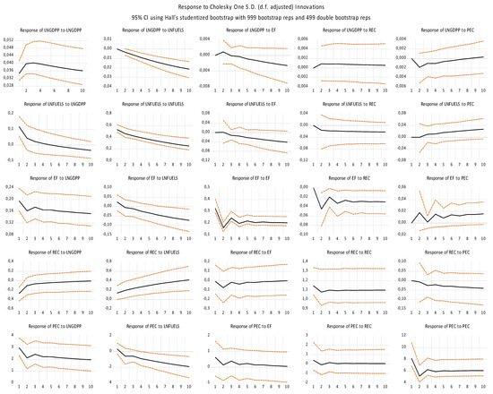
Figure 2.
Impulse Response Functions.
The response of the Ecological Footprint (EF) to shocks in other variables exhibits diverse patterns. In the case of a shock to GDP per capita (LNGDPPC), EF initially responds negatively until the second period, then turns positive until the third period, after which it becomes negative again. A shock in fuel exports (LNFUELS) leads to a consistently negative response, suggesting that increased fuel exports may worsen environmental outcomes. When EF is exposed to shocks in its own past values and renewable energy consumption (REC), the response is initially negative until the second period, becomes positive until the third period, turns negative again between the third and fourth periods, and shifts back to a positive response from the fourth to fifth periods. After the fifth period, the response levels off and moves parallel to the horizontal axis, indicating stabilization. In response to a shock in primary energy consumption (PEC), EF first reacts positively, then negatively, and continues in a zigzag pattern up to the eighth period, eventually stabilizing and aligning with the horizontal axis. The impulse response of renewable energy consumption (REC) to various shocks displays distinct patterns. In response to a shock in GDP per capita (LNGDPPC), REC shows a strong initial positive reaction, which gradually weakens and moves closer to a stable path, indicating a long-term alignment with the horizontal axis. Shocks in fuel exports (LNFUELS) lead to a consistently positive response, suggesting a complementary relationship. In the case of ecological footprint (EF), REC initially reacts negatively until the second period, turns positive in the third period, then mildly negative by the fourth, followed by a slight positive trend that stabilizes near the horizontal axis. When REC is exposed to its own shocks, the response is initially negative until the second period, becomes positive until the third, and then stabilizes. Lastly, a shock in primary energy consumption (PEC) results in a negative response, indicating that increases in overall energy use may not support renewable energy consumption in the short to medium term.
The impulse response of primary energy consumption (PEC) to shocks in other variables reveals diverse dynamics. In response to shocks in GDP per capita (LNGDPPC), renewable energy consumption (REC), and its own past values, PEC initially reacts negatively until the second period, turns positive in the third period, and then stabilizes. A shock to fuel exports (LNFUELS) leads to a consistently negative response, suggesting that an increase in fuel exports may be associated with reduced primary energy consumption. When faced with a shock in the ecological footprint (EF), PEC responds negatively until the second period, becomes positive by the third, and then shifts to a mildly negative path.
3.7. Short-Run Dynamics: Granger Causality
To investigate the short-run causal relationships among the variables, the VEC Granger Causality Exogeneity Wald test was employed, as suggested by Engle & Granger. The optimal lag length in the VECM was determined using the (AIC) and the (SC), both of which suggested that lag 1 was optimal. The null hypothesis in each case states shows that the excluded variable fails to Granger-cause the dependent variable in the short run.
The results, presented in Table 13, indicate that for the dependent variable D(LNGDPP), none of the independent variables—fuel exports (D(LNFUELS)), environmental footprint (D(EF)), renewable energy consumption (D(REC)), or primary energy consumption (D(PEC))—exhibit a statistically significant Granger causal effect, suggesting no short-run causality from these variables to economic growth. In the case of D(LNFUELS), only D(LNGDPP) shows a marginal effect with a p-value of 0.0774, suggesting a weak indication of short-run causality from economic growth to fuel exports. However, this effect is not strong enough to be conclusive at conventional significance levels. For the dependent variable D(EF), economic growth (D(LNGDPP)) and renewable energy consumption (D(REC)) both demonstrate statistically significant Granger causality at the 5% level, with p-values of 0.0239 and 0.0203, respectively. This implies that changes in GDP per capita and renewable energy use contribute to short-run variations in environmental pressure. Similarly, for D(REC), economic growth (D(LNGDPP)) Granger-causes renewable energy consumption at the 5% level (p = 0.0192), indicating a short-run relationship where economic activity influences renewable energy usage. No statistically significant short-run causality is found for the dependent variable D(PEC), suggesting that primary energy consumption is not significantly influenced by any of the other variables in the short run. Overall, the short-run Granger causality analysis highlights the importance of economic growth in explaining short-term fluctuations in environmental indicators, particularly environmental footprint and renewable energy consumption. However, other relationships appear to be weak or statistically insignificant in the short run.
Table 13.
VEC Tests.
3.8. Long-Run Dynamics: Fully Modified OLS & and Dynamic OLS
To explore the long-run dynamics of the variables under study, this section employs advanced panel data techniques, specifically the FMOLS and Dynamic OLS estimators. These estimators are renowned for their ability to address critical issues such as endogeneity and serial correlation in the error terms, which are common challenges in time series and panel data analysis. Both FMOLS and DOLS are derived from the Canonical Cointegrating Regression (CCR) approach and have been widely acknowledged for providing asymptotically unbiased and consistent estimates in the context of cointegration [68,69]. While FMOLS effectively corrects for endogeneity and serial correlation in the cointegrating regression, DOLS enhances the estimation by incorporating leads and lags of the different explanatory variables, further addressing potential endogeneity issues. These estimators are extensively used in empirical research for estimating long-run relationships in panel data settings, offering reliable and dependable results when cointegration is present. Additionally, both methods are consistent with the maximum likelihood estimation framework proposed by Johansen, ensuring their validity and r reliability in applied econometrics.
The results from the Panel DOLS and FMOLS models presented in Table 14 provide comprehensive insights into the long-term effects of various factors on GDP per capita (LNGDPP) in Poland. Both models consistently show that fuel exports (LNFUELS) have a positive and statistically significant impact on GDP per capita. Specifically, a 1% increase in fuel exports results in a 0.0493% increase in LNGDPP according to the DOLS model, and a 0.0604% increase in the FMOLS model. Similarly, the ecological footprint (EF) demonstrates a significant positive effect on DP per capita, with a 1% increase in EF leading to a 0.1365% increase in LNGDPP in the DOLS model and a 0.1173% increase in FMOLS. Renewable energy consumption (REC) also exhibits a positive and economically meaningful association with GDP per capita, with a 1% increase in REC resulting in a 0.0241% increase in LNGDPP in DOLS and a 0.02197% increase in FMOLS. In contrast, primary energy consumption (PEC) exhibits a very weak and statistically insignificant effect on GDP per capita in both models, with coefficients of 0.001106 in DOLS and 0.000339 in FMOLS, and neither relationship is significant (p-value > 0.05). The models’ high R-squared values—0.996341 for DOLS and 0.905 for FMOLS—indicate that they explain a substantial portion of the variation in GDP per capita. These findings emphasize the significant roles of fuel exports, ecological footprint, and REC in driving economic growth, while PEC shows a negligible impact.
Table 14.
DOLS and FMOLS Estimators.
In Table 15, the results from both the DOLS (Dynamic Ordinary Least Squares) and FMOLS (Fully Modified Least Squares) models are presented to assess the long-term relationships between variables and the ecological footprint (EF). The analysis indicates that GDP per capita (LNGDPP) consistently shows a positive and statistically significant effect on EF in both models. In the DOLS model, a 1% increase in GDP per capita leads to a 3.12% increase in EF, while in the FMOLS model, the effect is slightly lower, at 2.50%, suggesting a strong link between economic growth and rising environmental degradation. Conversely, Poland’s fuel exports (LNFUELS) do not significantly affect EF in either model. In DOLS, the coefficient for fuel exports is positive but statistically insignificant (p-value = 0.8275), and in FMOLS, it shows a similar insignificant relationship (p-value = 0.0469). The consumption of renewable energy (REC) presents an interesting finding, as it consistently shows a negative and significant relationship with EF in both models. In DOLS, a 1% increase in renewable energy consumption results in a 0.05% reduction in EF, while in FMOLS, this impact is slightly more pronounced at 0.061%, indicating that renewable energy consumption contributes to reducing environmental degradation. Lastly, primary energy consumption (PEC) shows a positive effect on EF in both models. In DOLS, a 1% increase in primary energy consumption leads to a 0.02% increase in EF, and in FMOLS, the effect is slightly higher at 0.02%. The R-squared values for both models are quite high, with DOLS reporting 0.967 and FMOLS showing 0.905, indicating that both models explain a significant portion of the variations in EF. In summary, both DOLS and FMOLS models show consistent findings regarding the significant impact of economic growth and primary energy consumption on EF, while renewable energy consumption plays a crucial role in reducing ecological pressures. These results provide important insights into the long-term relationships between energy consumption, economic growth, and environmental sustainability.
Table 15.
DOLS & FMOLS Estimators.
4. Discussion
This study investigates the relationship between EG, EC, and ED in Poland over the period 2000–2022. It integrates both short-run and long-run analyses by employing advanced econometric techniques such as the Vector Error Correction Model, Granger Causality tests, and long-run estimators like Fully Modified Ordinary Least Squares and Dynamic Ordinary Least Squares. The analysis focuses on valuable variables, including GDP per capita, fuel exports, ecological footprint, renewable energy consumption, and primary energy consumption. The findings provide valuable insights into how energy consumption and environmental factors influence Poland’s economic performance.
The short-run dynamics, as revealed in Table 13 by the Granger causality analysis based on the VECM, show selective interactions among the variables. Notably, GDP per capita Granger causes both the ecological footprint (EF) and renewable energy consumption (REC), with p-values of 0.0239 and 0.0192, respectively. This suggests that economic activity affects both environmental degradation and the demand for renewable energy in the short run. Moreover, the Granger causality test shows that REC Granger-causes EF (p = 0.0203), indicating a short-run feedback loop between renewable energy use and environmental quality. Interestingly, no significant short-run causality is detected between LNGDPP and conventional energy variables such as fuel exports and primary energy consumption (PEC), suggesting that economic activity affects environmental outcomes and renewable energy consumption more directly than conventional energy consumption in the short term. These findings align with existing literature that distinguishes between renewable and non-renewable energy sources. Studies such as [70,71] suggest that renewable energy has a smaller environmental impact and contributes more positively to sustainability. The results also echo findings by [42,72], who highlight the relatively lower ecological burden of renewable energy. Furthermore, the long-run relationships between energy consumption and economic growth mirror the findings of [26,29], particularly for upper-middle-income countries like Poland. However, the absence of a clear inverted U-shaped relationship between income and environmental degradation casts partial doubt on the Environmental Kuznets Curve (EKC) hypothesis, a finding that is also consistent with the mixed results reported by [73,74,75,76].
In the long-run cointegration equations derived from the VECM in Table 10, the dependent variable LNGDPP is influenced negatively by fuel exports, the ecological footprint (EF), and renewable energy consumption (REC), with coefficients of −0.6658, −0.2775, and −0.0238, respectively. These findings indicate that higher fuel exports, a larger ecological footprint, and increased renewable energy consumption are associated with lower economic growth. Conversely, primary energy consumption (PEC) positively impacts economic growth with a coefficient of 6.0062, suggesting that greater energy consumption supports economic growth. On the other hand, the ecological footprint (EF) is negatively affected by economic growth, fuel exports, and renewable energy consumption in the long run, with coefficients of −3.603070, −2.398765, and −0.085736, respectively. However, primary energy consumption increases the ecological footprint (coefficient of 0.022181), highlighting the environmental burden of higher energy consumption. These findings align with existing literature that documents the complex and sometimes contradictory interactions between energy consumption, environmental degradation, and economic growth. For instance, studies which report similar negative effects of fossil fuel exports and ecological footprint on growth, while highlighting the positive role of primary energy consumption in promoting economic activity [30,42,71]. At the same time, the environmental burden of higher energy consumption is widely recognized in the works of [17] and other scholars, who stress the need for sustainable energy policies to mitigate ecological damage.
The long-run analysis conducted through FMOLS and DOLS models indicates that ecological footprint, and renewable energy consumption exert a positive and consistent influence on GDP per capita, while the effect of fuel exports varies across models. Specifically, a 1% increase in fuel exports results in a 0.0493% to 0.0604% increase in GDP per capita, depending on the model. Similarly, a 1% increase in the environmental footprint leads to a 0.1365% to 0.1173% increase in economic growth, and renewable energy consumption contributes to a 0.0241% to 0.02197% increase in GDP per capita. These results align with existing literature that emphasizes the positive relationship between energy exports, economic growth, and environmental degradation. Fuel exports can stimulate economic growth by boosting industrial production and foreign exchange earnings, which contribute to higher national income, as noted by [77]. Additionally, the positive relationship between the environmental footprint and economic growth is consistent with the Environmental Kuznets Curve (EKC) hypothesis, which suggests that economic growth initially leads to environmental degradation, but this relationship reverses at higher income levels and with effective environmental policies. However, primary energy consumption appears to have a limited effect on economic growth in the long run, as shown by the weak and statistically insignificant coefficients across both DOLS and FMOLS estimations.
This suggests that while primary energy consumption is important for development, its direct impact on GDP per capita may be less pronounced than that of fuel exports and renewable energy consumption. This finding contrasts with studies such as Apergis and Payne [78], which emphasize the importance of primary energy consumption for economic growth, suggesting that the energy mix and energy efficiency are critical in determining this relationship. One notable finding from the long-run analysis is the strong and positive relationship between GDPs per capita and the ecological footprint. The DOLS and FMOLS results in Table 15 indicate that a 1% increase in GDP per capita leads to a 3.12% and 2.50% increase in the ecological footprint, respectively. This highlights the challenge of balancing economic growth with environmental sustainability, particularly in rapidly industrializing countries like Poland. The significant impact of economic growth on the ecological footprint suggests that expanding economies may increase resource consumption and environmental degradation. However, renewable energy consumption is shown to mitigate some of this effect. Both DOLS and FMOLS results indicate that a 1% increase in renewable energy consumption reduces the ecological footprint, underscoring the potential of renewable energy to decouple economic growth from environmental degradation. This finding supports the growing body of literature suggesting that renewable energy adoption can help reduce the environmental impact of economic growth and contribute to sustainable development [79].
The findings of this study carry several important implications for policymakers aiming to balance economic growth with environmental sustainability in Poland. First, the significant short-run causality from GDP per capita to both ecological footprint and renewable energy consumption indicates that economic activity directly influences environmental pressures and energy demand patterns. Consequently, policy measures should integrate economic development plans with environmental management strategies to ensure sustainable growth. Given the positive feedback loop identified between renewable energy consumption and ecological footprint, policymakers are encouraged to promote investments in renewable energy infrastructure and technology. Expanding renewable energy use can mitigate environmental degradation while supporting the economy, highlighting the critical role of clean energy policies in Poland’s transition towards sustainable development.
The long-run results suggest a complex interaction where fuel exports and the ecological footprint negatively impact economic growth, while primary energy consumption positively supports it. This indicates a need for a nuanced energy policy that reduces reliance on fossil fuel exports, which may hamper sustainable economic performance, while optimizing primary energy consumption through efficiency improvements and diversification of energy sources. Moreover, the observed positive relationship between economic growth and ecological footprint in the long run underscores the ongoing challenge of reconciling growth objectives with environmental protection. Policymakers should strengthen environmental regulations and adopt green growth strategies that encourage sustainable resource use and pollution control without constraining economic progress. The insignificant long-run effect of primary energy consumption on GDP per capita suggests that energy efficiency and the energy mix are pivotal. Thus, policies fostering energy efficiency improvements and increasing the share of renewables in the energy portfolio should be prioritized.
Finally, the evidence that renewable energy consumption reduces the ecological footprint points to the importance of sustained support for renewable energy development. Incentives such as subsidies, tax breaks, and research funding for renewable technologies could accelerate their adoption, thereby facilitating decoupling of economic growth from environmental degradation. In summary, integrated policy frameworks that simultaneously address energy consumption patterns, environmental sustainability, and economic growth dynamics are essential for Poland to achieve long-term sustainable development goals.
The results of this study suggest several key policy directions for Poland to harmonize economic growth with environmental sustainability. The short-run causality from GDP per capita to ecological footprint and renewable energy consumption underscores the direct impact of economic activity on environmental outcomes and energy demand, indicating that economic policies should be integrated with environmental considerations to foster sustainable development [16]. The identified bidirectional relationship between renewable energy consumption and ecological footprint emphasizes the importance of promoting renewable energy. Policymakers should incentivize investments in renewable energy infrastructure and technology as a means to reduce environmental degradation while supporting economic growth [5]. Such policies align with global sustainable development goals and help Poland transition toward a low-carbon economy [39].
Long-run findings reveal that while fuel exports and ecological footprint negatively affect economic growth, primary energy consumption exerts a positive effect. This suggests that Poland’s energy policy should focus on reducing dependence on fossil fuel exports, which may hinder sustainable growth, and enhancing energy efficiency and diversification in the energy mix [28]. Moreover, the weak long-run impact of primary energy consumption on GDP growth points to the vital role of energy efficiency and cleaner energy sources in sustaining economic development [80]. Therefore, policy measures should prioritize improvements in energy efficiency and the expansion of renewable energy to reduce environmental harm and foster sustainable growth [81].
5. Conclusions
This research investigated the complex interactions between economic growth, renewable and non-renewable energy consumption, and environmental sustainability across Poland’s 18 primary energy-importing partner countries during the period 2000 to 2022. Utilizing a robust methodological approach—including Vector Error Correction Model (VECM), Fully Modified Ordinary Least Squares (FMOLS), Dynamic Ordinary Least Squares (DOLS), Granger Causality tests, and impulse-response analysis—the study uncovered both short-term and long-term dynamic relationships among the variables.
The findings reveal that fuel exports, renewable energy consumption, and ecological footprint significantly influence GDP per capita growth in the long run. Renewable energy consumption plays a dual role by supporting economic growth while simultaneously mitigating environmental degradation. Conversely, primary (fossil-based) energy consumption shows no significant impact on economic growth, indicating that mere increases in energy usage do not effectively drive development. The positive association between ecological footprint and GDP per capita highlights a clear trade-off between economic expansion and environmental health, raising important sustainability concerns. Regarding the study’s hypotheses:
Hypothesis 1 posits that an energy supply shock originating from Poland adversely affects the economic growth of dependent countries while simultaneously increasing their ecological footprints. Based on the results from DOLS and FMOLS estimations (Table 14 and Table 15), the Poland fuel exports variable (LNFUELS) has a positive and statistically significant effect on economic growth (LNGDPP). This indicates that energy shocks from Poland do not reduce economic growth; rather, they are associated with an increase in GDP per capita. Regarding the impact on ecological footprint (EF), LNFUELS shows an insignificant effect in the DOLS model and a negative significant effect in the FMOLS model, suggesting no evidence of increased environmental pressure due to Poland’s fuel exports. Therefore, Hypothesis 1 is not supported in this study, as energy supply shocks from Poland neither hinder economic growth nor exacerbate environmental degradation.
Hypothesis 2 suggests that substituting imported fossil-based energy with domestic renewable energy consumption (REC) promotes economic growth without intensifying environmental degradation. The results from DOLS and FMOLS estimations show that renewable energy consumption (REC) has a positive and statistically significant effect on GDP per capita (LNGDPP). This confirms that increased use of renewable energy supports long-term economic growth. Additionally, REC exhibits a negative and significant impact on the ecological footprint (EF), indicating that renewable energy consumption contributes to environmental sustainability by reducing environmental pressure. Thus, the evidence supports Hypothesis 2, demonstrating that a shift towards domestic renewable energy fosters sustainable economic development without worsening ecological conditions.
These findings have important policy implications: Prioritizing investments in renewable energy infrastructure is essential to support sustainable economic growth while reducing environmental harm. Enhancing energy efficiency and reducing dependency on fossil fuel imports through diversification and domestic renewable energy deployment will improve energy security and resilience. Integrating environmental constraints into economic planning frameworks can help reconcile the trade-off between growth and ecological sustainability. For Poland and its energy-importing partners, a strategic transition toward cleaner energy sources and sustainable export policies is crucial to ensuring economic growth does not exacerbate environmental challenges.
Overall, the findings of this study are particularly relevant for policymakers in energy-importing countries from Poland and environmental economists working on energy and sustainable development issues. However, it should be emphasized that the results are primarily generalizable to countries with similar institutional structures, energy policies, and trade patterns as these importing countries. Extending these findings to other regions with different governance frameworks and varying degrees of fossil fuel dependency require careful consideration and contextual adaptation. Acknowledging these limitations enhances the transparency and practical relevance of the policy recommendations, helping decision-makers design more effective energy and sustainability policies tailored to local conditions.
Author Contributions
Conceptualization, M.T.N.; methodology, M.T.N. and A.K.; software, M.T.N.; validation, M.T.N., A.B.-B. and A.K.; formal analysis, M.T.N. and A.K.; investigation, M.T.N. and A.K.; resources, M.T.N.; data curation, M.T.N.; writing—original draft preparation, M.T.N., A.B.-B., P.B. and T.R.; writing—review and editing, M.T.N., A.B.-B., P.B., T.R. and A.K.; visualization, M.T.N.; supervision, M.T.N.; project administration, M.T.N. and A.B.-B. All authors have read and agreed to the published version of the manuscript.
Funding
The results presented in this paper were not funded.
Data Availability Statement
Data are contained within the article.
Conflicts of Interest
The authors declare no conflicts of interest.
Abbreviations
The following abbreviations are used in this manuscript:
| EG | economic growth |
| GDP | Gross Domestic Product |
| SDGs | Sustainable Development Goals |
| EKC | Environmental Kuznets Curve |
| ED | environmental degradation |
| PVAR | Panel Vector Autoregression |
| FMOLS | Fully Modified Ordinary Least Squares |
| DOLS | Dynamic Ordinary Least Squares |
References
- Intergovernmental Panel on Climate Change (IPCC). Summary for Policymakers; Cambridge University Press: Cambridge, UK, 2018. [Google Scholar] [CrossRef]
- Adams, S.; Acheampong, A.O. Reducing carbon emissions: The role of renewable energy and democracy. J. Clean. Prod. 2019, 240, 118245. [Google Scholar] [CrossRef]
- Wang, Z.; Ahmed, Z.; Zhang, B.; Wang, B. The nexus between urbanization, road infrastructure, and transport energy demand: Empirical evidence from Pakistan. Environ. Sci. Pollut. Res. 2019, 26, 34884–34895. [Google Scholar] [CrossRef] [PubMed]
- Rafindadi, A.A.; Yusof, Z.; Zaman, K.; Kyophilavong, P.; Akhmat, G. The relationship between air pollution, fossil fuel energy consumption, and water resources in the panel of selected Asia-Pacific countries. Environ. Sci. Pollut. Res. 2014, 21, 11395–11400. [Google Scholar] [CrossRef]
- Pata, U.K. The influence of coal and noncarbohydrate energy consumption on CO2 emissions: Revisiting the environmental Kuznets curve hypothesis for Turkey. Energy 2018, 160, 1115–1123. [Google Scholar] [CrossRef]
- Das, D.; Srinivasan, R.; Sharfuddin, A. Fossil fuel consumption, carbon emissions and temperature variation in India. Energy Environ. 2011, 22, 695–709. [Google Scholar] [CrossRef]
- Alkhathlan, K.; Javid, M. Energy consumption, carbon emissions and economic growth in Saudi Arabia: An aggregate and disaggregate analysis. Energy Policy 2013, 62, 1525–1532. [Google Scholar] [CrossRef]
- Yuping, L.; Ramzan, M.; Xie, Y.; Jawad, M.; Sharif, A.; Irfan, M. Determinants of carbon emissions in Argentina: The roles of renewable energy consumption and globalization. Energy Rep. 2021, 7, 4747–4760. [Google Scholar] [CrossRef]
- Kılıç Depren, S.; Kartal, M.T.; Çoban Çelikdemir, N.; Depren, Ö. Energy consumption and environmental degradation nexus: A systematic review and meta-analysis of fossil fuel and renewable energy consumption. Ecol. Inform. 2022, 70, 101747. [Google Scholar] [CrossRef]
- Dong, K.; Sun, R.; Li, H.; Liao, H. Does natural gas consumption mitigate CO₂ emissions: Testing the environmental Kuznets curve hypothesis for 14 Asia-Pacific countries. Renew. Sustain. Energy Rev. 2018, 94, 419–429. [Google Scholar] [CrossRef]
- Ramzan, M.; Raza, S.A.; Usman, M.; Sharma, G.D.; Iqbal, H.A. Environmental cost of non-renewable energy and economic progress: Do ICT and financial development mitigate some burden? J. Clean. Prod. 2022, 333, 130066. [Google Scholar] [CrossRef]
- Cheng, K.; Hsueh, H.P.; Ranjbar, O.; Wang, M.C.; Chang, T. Urbanization, coal consumption and CO₂ emissions nexus in China using bootstrap Fourier Granger causality test in quantiles. Lett. Spat. Resour. Sci. 2021, 14, 31–49. [Google Scholar] [CrossRef]
- Lim, K.M.; Lim, S.Y.; Yoo, S.H. Oil consumption, CO₂ emission, and economic growth: Evidence from the Philippines. Sustainability 2014, 6, 967–979. [Google Scholar] [CrossRef]
- Saboori, B.; Rasoulinezhad, E.; Sung, J. The nexus of oil consumption, CO₂ emissions and economic growth in China, Japan and South Korea. Environ. Sci. Pollut. Res. 2017, 24, 7436–7455. [Google Scholar] [CrossRef]
- Huang, Y.; Xue, L.; Khan, Z. What abates carbon emissions in China: Examining the impact of renewable energy and green investment. Sustain. Dev. 2021, 29, 823–834. [Google Scholar] [CrossRef]
- Farhani, S.; Shahbaz, M. What role of renewable and non-renewable electricity consumption and output is needed to initially mitigate CO2 emissions in MENA region? Renew. Sustain. Energy Rev. 2014, 40, 80–90. [Google Scholar] [CrossRef]
- Zafar, M.W.; Shahbaz, M.; Hou, F.; Sinha, A. From nonrenewable to renewable energy and its impact on economic growth: The role of research & development expenditures in Asia-Pacific Economic Cooperation countries. J. Clean Prod. 2019, 212, 1166–1178. [Google Scholar] [CrossRef]
- Faizi, A.; AK, M.Z.; Shahzad, M.R.; Yüksel, S.; Toffanin, R. Environmental Impacts of Natural Resources, Renewable Energy, Technological Innovation, and Globalization: Evidence from the Organization of Turkic States. Sustainability 2024, 16, 9705. [Google Scholar] [CrossRef]
- Altıntaş, N.; Açıkgöz, F.; Okur, M.; Öztürk, M.; Aydın, A. Renewable Energy and Banking Sector Development Impact on Load Capacity Factor in Malaysia. J. Clean Prod. 2024, 434, 140143. [Google Scholar] [CrossRef]
- Acaravcı, A.; Erdoğan, S. Renewable Energy, Environment and Economic Growth Nexus: An Empirical Analyses for Selected Countries. Eskişehir Osman. Üniversitesi İktisadi ve İdari Bilim. Derg. 2018, 13, 53–64. [Google Scholar] [CrossRef]
- Danish, R.; Ulucak, S.U.D.; Khan, M.A.; Baloch, N.; Li, N. Mitigation pathways toward sustainable development: Is there any trade-off between environmental regulation and carbon emissions reduction? Sustain. Dev. 2020, 28, 813–822. [Google Scholar] [CrossRef]
- Shahzad, U. Environmental taxes, energy consumption, and environmental quality: Theoretical survey with policy implications. Environ. Sci. Pollut. Res. 2020, 27, 24848–24862. [Google Scholar] [CrossRef] [PubMed]
- Murshed, M.; Rahman, M.A.; Alam, S.; Ahmad, P.; Dagar, V. The nexus between environmental regulations, economic growth, and environmental sustainability: Linking environmental patents to ecological footprint reduction in South Asia. Environ. Sci. Pollut. Res. 2021, 28, 49967–49988. [Google Scholar] [CrossRef] [PubMed]
- Sun, H.; Liu, Z.; Chen, Y. Foreign direct investment and manufacturing pollution emissions: A perspective from heterogeneous environmental regulation. Sustain. Dev. 2020, 28, 1376–1387. [Google Scholar] [CrossRef]
- Fotis, P.; Polemis, M. Sustainable development, environmental policy and renewable energy use: A dynamic panel data approach. Sustain. Dev. 2018, 26, 726–740. [Google Scholar] [CrossRef]
- Yaşar, N. The relationship between energy consumption and economic growth: Evidence from different income country groups. Int. J. Energy Econ. Policy 2017, 7, 86–97. Available online: http://www.econjournals.com (accessed on 22 June 2025).
- Wolde-Rufael, Y. Electricity consumption and economic growth: A time series experience for 17 African countries. Energy Policy 2006, 34, 1106–1114. [Google Scholar] [CrossRef]
- Tang, C.F.; Tan, B.W.; Ozturk, I. Energy consumption and economic growth in Vietnam. Renew. Sustain. Energy Rev. 2016, 54, 1506–1514. [Google Scholar] [CrossRef]
- Amri, F. The relationship amongst energy consumption (renewable and non-renewable), and GDP in Algeria. Renew. Sustain. Energy Rev. 2017, 76, 62–71. [Google Scholar] [CrossRef]
- Yildirim, E.; Saraç, Ş.; Aslan, A. Energy consumption and economic growth in the USA: Evidence from renewable energy. Renew. Sustain. Energy Rev. 2012, 16, 6770–6774. [Google Scholar] [CrossRef]
- Pirlogea, C.; Cicea, C. Econometric perspective of the energy consumption and economic growth relation in European Union. Renew. Sustain. Energy Rev. 2012, 16, 5718–5726. [Google Scholar] [CrossRef]
- Belke, A.; Dobnik, F.; Dreger, C. Energy consumption and economic growth: New insights into the cointegration relationship. Energy Econ. 2011, 33, 782–789. [Google Scholar] [CrossRef]
- Eggoh, J.C.; Bangaké, C.; Rault, C. Energy Consumption and Economic Growth Revisited in African Countries. Energy Policy 2011, 39, 7408–7421. [Google Scholar] [CrossRef]
- Hondroyiannis, G.; Lolos, S.; Papapetrou, E. Energy consumption and economic growth: Assessing the evidence from Greece. Energy Econ. 2002, 24, 319–336. [Google Scholar] [CrossRef]
- Wackernagel, M.; Silverstein, J. Big things first: Focusing on the scale imperative with the ecological footprint. Ecol. Econ. 2000, 32, 391–394. Available online: www.elsevier.com/locate/ecolecon (accessed on 16 May 2025).
- Brundtland, G.H. Report of the World Commission on Environment and Development: Our Common Future. In Ecological Economics; Elsevier: Amsterdam, The Netherlands, 1987; Available online: https://sustainabledevelopment.un.org/content/documents/5987our-common-future.pdf (accessed on 10 May 2025).
- Koyuncu, T.; Karabulut, T. Sustainable Development and Green Economy in Turkey in Terms of Renewable Energy: An Empirical Study. Int. J. Manag. Econ. Bus. 2021, 17, 2. [Google Scholar] [CrossRef]
- Global Footprint Network. Global Footprint Network. 2022. Available online: https://data.footprintnetwork.org/?_ga=2.163631420.2019855520.1651002862-486537495.1649423688#/ (accessed on 10 May 2025).
- International Energy Agency (IEA). Renewables 2024: Analysis and Forecast to 2030; International Energy Agency (IEA): Paris, France, 2024; Available online: https://www.iea.org/reports/renewables-2024 (accessed on 1 May 2025).
- Eurostat. Renewable Energy Statistics. Available online: https://ec.europa.eu/eurostat/statistics-explained/index.php?title=Renewable_energy_statistics#Share_of_renewable_energy_more_than_doubled_between_2004_and_2020 (accessed on 1 May 2025).
- International Energy Agency, IEA. Russian Supplies to Global Energy Markets. 2022. Available online: https://www.iea.org/reports/russian-supplies-to-global-energy-markets (accessed on 1 May 2025).
- Öncel, A.; Kabasakal, A.; Kutlar, A.; Acar, S. Energy consumption, economic growth and Ecological footprint relationship in the top Russian energy importers: A panel data analysis. Environ. Dev. Sustain. 2024, 26, 21019–21052. [Google Scholar] [CrossRef]
- Engle, R.F.; Granger, C.W.J. Co-integration and error correction: Representation, estimation, and testing. Econometrica 1987, 55, 251–276. [Google Scholar] [CrossRef]
- Pedroni, P. Critical values for cointegration tests in heterogeneous panels with multiple regressors. Oxf. Bull. Econ. Stat. 1999, 61, 653–670. [Google Scholar] [CrossRef]
- Love, I.; Zicchino, L. Financial development and dynamic investment behavior: Evidence from panel VAR. Q. Rev. Econ. Finance. 2006, 46, 190–210. [Google Scholar] [CrossRef]
- Barbieri, L. Panel Unit Root Tests Under Cross-Sect. Depend.: An overview. J. Stat. Adv. Theory Appl. 2009, 1, 117–158. Available online: https://www.researchgate.net/publication/267090484 (accessed on 16 May 2025).
- Levin, A.; Lin, C.-F.; Chu, C.-S.J. Unit root tests in panel data: Asymptotic and finite-sample properties. J. Econ. 2002, 108, 1–24. [Google Scholar] [CrossRef]
- Im, K.S.; Pesaran, M.H. On the Panel Unit Root Tests Using Nonlinear Instrumental Variables. SSRN 482463. 2003 Oct.
- Maddala, G.S.; Wu, S. A comparative study of unit root tests with panel data and a new simple test. Oxf. Bull. Econ. Stat. 1999, 61, 631–652. [Google Scholar] [CrossRef]
- Hadri, K. Testing for stationarity in heterogeneous panel data. Econom. J. 2000, 3, 148–161. [Google Scholar] [CrossRef]
- Pesaran, M.H. A simple panel unit root test in the presence of cross-section dependence. J. Appl. Econom. 2007, 22, 265–312. [Google Scholar] [CrossRef]
- Moon, H.R.; Perron, B. Testing for a unit root in panels with dynamic factors. J. Econom. 2004, 122, 81–126. [Google Scholar] [CrossRef]
- Smith, L.V.; Leybourne, S.; Kim, T.H.; Newbold, P. More powerful panel data unit root tests with an application to mean reversion in real exchange rates. J. Appl. Econom. 2004, 19, 147–170. [Google Scholar] [CrossRef]
- Carrion-I-Silvestre, J.L.; Del Barrio-Castro, T.; López-Bazo, E. Breaking the panels. An application to the GDP per capita. Working Paper No. 97. Econom. J. 2003, 8, 159–175. [Google Scholar] [CrossRef]
- Banerjee, A.; Guo, X.; Wang, H. On the optimality of conditional expectation as a Bregman predictor. IEEE Trans. Inf. Theory 2005, 51, 2664–2669. [Google Scholar] [CrossRef]
- Pesaran, M.H. General diagnostic tests for cross-section dependence in panels. Empir. Econ. 2004, 60, 13–50. [Google Scholar] [CrossRef]
- Salim, R.A.; Rafiq, S. Why do some emerging economies proactively accelerate the adoption of renewable energy? Energy Econ. 2012, 34, 1051–1057. [Google Scholar] [CrossRef]
- Breusch, T.S.; Pagan, A.R. The Lagrange Multiplier Test and its Applications to Model Specification in Econometrics. Rev. Econ. Stud. 1980, 47, 239–253. [Google Scholar] [CrossRef]
- Baltagi, B.H.; Feng, Q.; Kao, C. A Lagrange Multiplier test for cross-sectional dependence in a fixed effects panel data model. J. Eco. 2012, 170, 164–177. [Google Scholar] [CrossRef]
- Pedroni, P. Panel cointegration: Asymptotic and finite sample properties of pooled time series tests with an application to the PPP hypothesis. Econ. Theory 2004, 20, 597–625. [Google Scholar] [CrossRef]
- WDI. The World Bank Groups. In World Development Indicators; The World Bank Groups: Washington, DC, USA; Available online: https://databank.worldbank.org/source/world-development-indicators (accessed on 12 May 2025).
- GFN. Global Footprint Network. In Advancing the Science of Sustainability; Global Footprint Network: Oakland, CA, USA; Available online: https://www.footprintnetwork.org (accessed on 12 May 2025).
- Noorzai, M.T. The impact of remittances on inflation in South Asian Association for Regional Cooperation (SAARC) countries. Sakarya. J. Econ. 2024, 13, 23–34. [Google Scholar]
- Bai, J.; Ng, S. A panic attack on unit roots and cointegration. Econometrica 2004, 72, 1127–1177. [Google Scholar] [CrossRef]
- Johansen, S. Estimation and Hypothesis Testing of Cointegration Vectors in Gaussian Vector Autoregressive Models. Econometrica 1991, 59, 1551–1580. [Google Scholar] [CrossRef]
- Johansen, S. A statistical analysis of cointegration for I(2) variables. Econom. Theory 1995, 11, 25–59. [Google Scholar] [CrossRef]
- Phillips, P.C.B.; Moon, H.R. Linear regression limit theory for nonstationary panel data. Econometrica 1999, 67, 1057–1111. [Google Scholar] [CrossRef]
- Kao, C. Spurious regression and residual-based tests for cointegration in panel data. J. Econ. 1999, 90, 1–44. [Google Scholar] [CrossRef]
- Pedroni, P. Purchasing power parity tests in cointegrated panels. Rev. Econ. Stat. 2001, 83, 727–731. [Google Scholar] [CrossRef]
- Murshed, M.; Nurmakhanova, M.; Al-Tal, R.; Mahmood, H.; Elheddad, M.; Ahmed, R. Can intra-regional trade, renewable energy use, foreign direct investments, and economic growth mitigate ecological footprints in South Asia? Energy Sources Part B Econ. Plan. Policy 2022, 17, 2038730. [Google Scholar] [CrossRef]
- Xiong, J.; Xu, D. Relationship between energy consumption, economic growth and environmental pollution in China. Environ. Res. 2021, 194, 110718. [Google Scholar] [CrossRef] [PubMed]
- Destek, M.A.; Sarkodie, S.A. Investigation of environmental Kuznets curve for ecological footprint: The role of energy and financial development. Sci. Total Environ. 2019, 650, 2483–2489. [Google Scholar] [CrossRef] [PubMed]
- Alola, A.A.; Bekun, F.V.; Sarkodie, S.A. Dynamic impact of trade policy, economic growth, fertility rate, renewable and non-renewable energy consumption on ecological footprint in Europe. Sci. Total Environ. 2019, 685, 702–709. [Google Scholar] [CrossRef]
- Alper, A.E.; Alper, F.O.; Ozayturk, G.; Mike, F. Testing the long-run impact of economic growth, energy consumption, and globalization on ecological footprint: New evidence from Fourier bootstrap ARDL and Fourier bootstrap Toda–Yamamoto test results. Environ. Sci. Pollut. Res. 2023, 30, 42873–42888. [Google Scholar] [CrossRef]
- Caviglia-Harris, J.L.; Chambers, D.; Kahn, J.R. Taking the ‘U’ out of Kuznets. A comprehensive analysis of the EKC and environmental degradation. Ecol. Econ. 2009, 68, 1149–1159. [Google Scholar] [CrossRef]
- Al-Mulali, U.; Weng-Wai, C.; Sheau-Ting, L.; Mohammed, A.H. Investigating the environmental Kuznets curve (EKC) hypothesis by utilizing the ecological footprint as an indicator of environmental degradation. Ecol. Indic. 2015, 48, 315–323. [Google Scholar] [CrossRef]
- Ahmed, Z.; Zhang, B.; Cary, M. Linking economic globalization, economic growth, financial development, and ecological footprint: Evidence from symmetric and asymmetric ARDL. Ecol. Indic. 2021, 121, 107060. [Google Scholar] [CrossRef]
- Apergis, N.; Payne, J.E. CO2 emissions, energy usage, and output in Central America. Energy Policy 2009, 37, 3282–3286. [Google Scholar] [CrossRef]
- Khan, A.; Chenggang, Y.; Bano, S.; Hussain, J. The empirical relationship between environmental degradation, economic growth, and social well-being in Belt and Road Initiative countries. Environ. Sci. Pollut. Res. 2020, 27, 30800–30814. [Google Scholar] [CrossRef]
- Kahia, M.; Ben Aïssa, M.S.; Charfeddine, L. Impact of renewable and non-renewable energy consumption on economic growth: New evidence from the MENA Net Oil Exporting Countries (NOECs). Energy 2016, 116, 102–115. [Google Scholar] [CrossRef]
- Udemba, E.N. A sustainable study of economic growth and development amidst ecological footprint: New insight from Nigerian perspective. Sci. Total Environ. 2020, 732, 139270. [Google Scholar] [CrossRef] [PubMed]
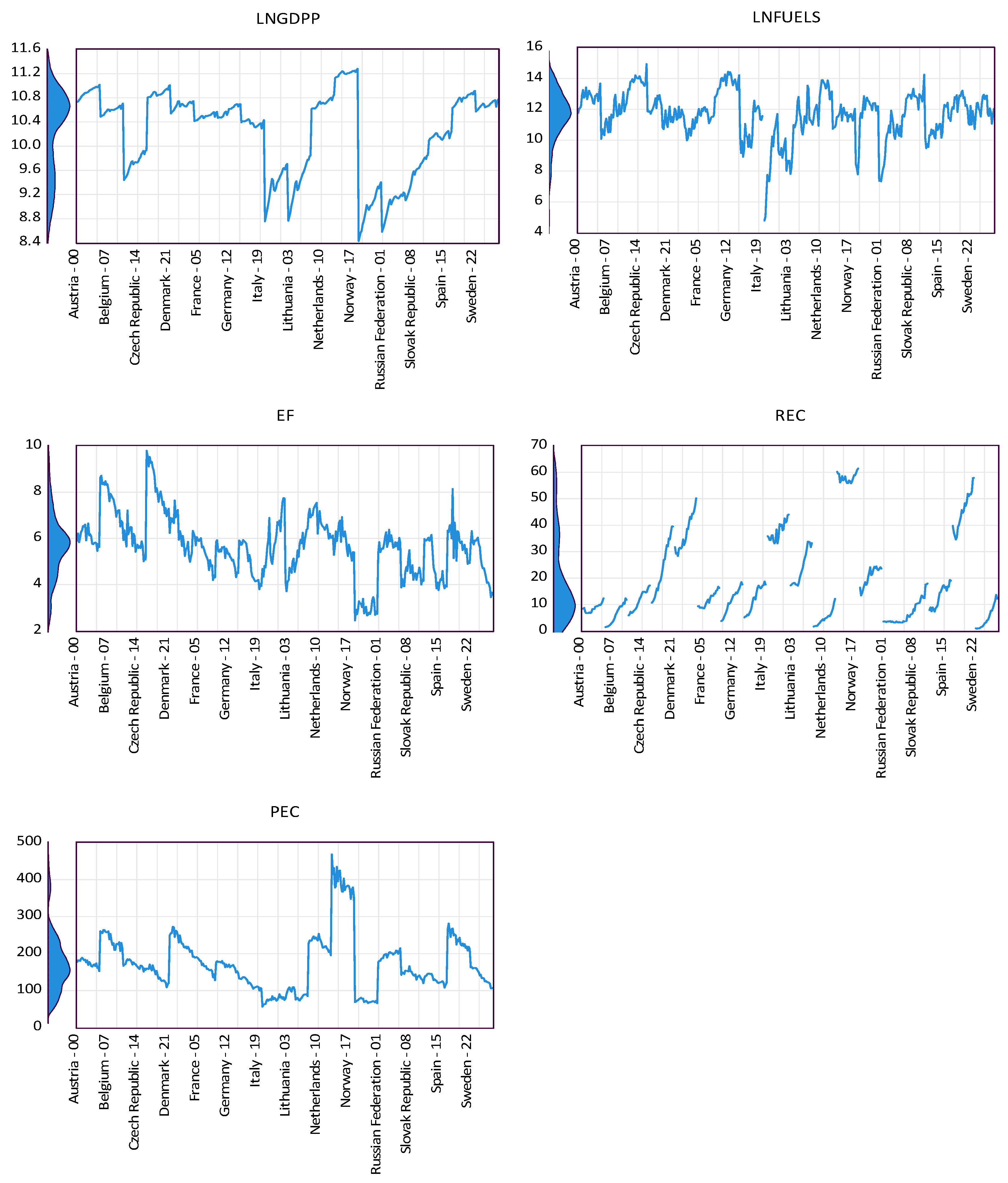

Disclaimer/Publisher’s Note: The statements, opinions and data contained in all publications are solely those of the individual author(s) and contributor(s) and not of MDPI and/or the editor(s). MDPI and/or the editor(s) disclaim responsibility for any injury to people or property resulting from any ideas, methods, instructions or products referred to in the content. |
© 2025 by the authors. Licensee MDPI, Basel, Switzerland. This article is an open access article distributed under the terms and conditions of the Creative Commons Attribution (CC BY) license (https://creativecommons.org/licenses/by/4.0/).