Article

Thermogravimetric Assessment and Kinetic Analysis of Forestry Residues Combustion

by
João Pedro Silva
1,2,*,
Senhorinha Teixeira
2 and
José Carlos Teixeira
1
1
MEtRICs Research Centre, University of Minho, 4800-058 Guimarães, Portugal
2
ALGORITMI Research Centre, LASI (Laboratório Associado de Sistemas Inteligentes), University of Minho, 4800-058 Guimarães, Portugal
*
Author to whom correspondence should be addressed.
Energies 2025, 18(13), 3299; https://doi.org/10.3390/en18133299
Submission received: 2 April 2025 / Revised: 10 June 2025 / Accepted: 19 June 2025 / Published: 24 June 2025

Abstract

The development of combustion experiments in a controlled environment is essential for comparing different fuels and quantifying the influence of different key parameters. It is fundamental to understand the transport phenomena at the particle level to obtain reliable results and information for further proper biomass combustion modeling of large-scale equipment. Hence, this paper presents a comprehensive analysis of the thermal decomposition and kinetic of eight samples of forest biomass fuels in terms of combustion behavior by using the thermogravimetric analysis (TGA) technique. The tests were carried out in an oxidizing atmosphere at a heating rate between 5 and 100 °C/min up to 900 °C. It was observed that, for all samples, fuel conversion follows a sequence of drying, devolatilization, and char combustion. Furthermore, differences in chemical and physical composition, as well as in structures and their thermal stability, justify the differences observed between the mass-loss curves of the different fuels. For this, the complexity of kinetic study is addressed in this paper by using different approaches: isoconversional and model-fitting methods. However, the use of isoconversional methods proved ineffective for determining reliable kinetic parameters, due to their sensitivity to particle conversion. A significant variation in activation energy was observed during the devolatilization stage, ranging from 47.92 to 101.30 kJ/mol. For the char oxidation stage, it ranged from 14.97 to 35.48 kJ/mol. These results highlight Eucalyptus as the most reactive species among those studied.

1. Introduction

The energy sector faces regulatory pressure, higher competition, and a demand to provide greater flexibility and environmentally friendly solutions. Due to this, at this time, it is necessary to respond effectively and rapidly to the fast-changing context of the electricity market. Motivated by its availability, widespread abundance, and environmental concerns, solid biomass has become a competitive option to diversify electricity production and direct heat among renewable energy resources [1]. However, although biomass is considered a sustainable, renewable, and CO2-neutral energy source [1], this characterization has been the subject of significant debate in recent years [2,3,4,5,6]. It is crucial to ensure that only residues from biomass, rather than whole harvested trees, are utilized. Promoting the use of biomass in the industrial sector can help reduce the amount of combustible material in woodlands, thereby lowering the risk of forest fires. This approach offers additional benefits for society, the environment, and the economy [7,8].
According to the last set of data for Portugal [9], in 2023 the contribution of biomass to renewable-energy production was approximately 42%. However, 60% of biomass has been converted into other forms of energy, specifically in cogeneration and dedicated power plants. Thus, biomass represents one of the main vectors contributing to the decarbonization of the primary energy demand and final energy consumption. Regarding these two parameters, biomass contribution is 40% and 36%, respectively, being the main renewable-energy source.
Combustion, the most usual conversion process of solid biomass, still requires further research since it is related to low efficiency and pollutants emissions [10,11]. This is particularly true if low-value fuels are used. Low-value fuels refer to biomass fuels with a high moisture content, high ash or inert content, and a significant proportion of non-wood components, such as bark and leaves. A need for the expansion of knowledge about alternative solid biomass fuels drives the need for the determination of the characteristics of such new energy sources. In recent decades, a lot of research has focused on TGA to study the thermal conversion of solid biomass, particularly considering pyrolysis among the different conversion technologies [12]. Thermogravimetric analysis is particularly suitable for studying biomass combustion as it enables accurate monitoring of mass loss during thermal decomposition, providing essential data to characterize reaction mechanisms and establishing reliable kinetic parameters for modeling combustion behavior.
The environmental atmosphere and the heating program are two crucial parameters influencing TGA. Non-isothermal experiments are generally adopted as they are considered more reliable for further studies and less time-consuming than isothermal experiments [5]. These experiments include information on the temperature dependence of the reaction rate, and it is commonly believed that it would be sufficient to derive the Arrhenius parameters and the reaction model of a process [6]. Consequently, the heating rate is one of the most relevant parameters in TGA as it affects thermal decomposition. Usually, experiments must be performed with several heating rates to solve possible compensation effects [7]. This is an important parameter as it greatly affects the volatiles’ release rate due to the thermal inertia of the particles, and, in this way, different heating rates should be applied in order to study its influence [8].
Regarding the ambient atmosphere, an oxidative atmosphere greatly affects the devolatilization behavior [9]. There are some works in the literature reporting the effect of this parameter [10,11,12]. For instance, according to Anca-Couce et al. [11] and Shen et al. [12], the presence of oxygen enhances biomass decomposition and promotes char combustion.
In the literature, TGA is not only the most usual thermoanalytical technique used for solid-phase thermal degradation studies but also for assessing the kinetics of the different reactions [13,14]. However, the determination of the kinetic parameters for biomass thermal degradation is particularly complicated considering the presence of complex components and their consecutive and/or parallel reactions. There are two main mathematical approaches to obtaining the kinetics data from the thermogravimetric analysis: (1) model-free methods (isoconversional) and (2) model-based methods [7]. In order to avoid modeling complex reactions, model-free methods can be preferable since the chemical parameters are determined without using any specific reaction model [15]. The model-free method generates unique kinetic parameters as a function of the conversion rate since they are based on the principle for each constant conversion; the reaction rate is a function only of the temperature [16].
Hence, reaction kinetics is based on the evaluation of the dependence of the effective activation energy (E), one of the Arrhenius parameters, on the conversion rate according to the TGA data at multiple heating rates, such as suggested by the International Confederation for Thermal Analysis and Calorimetry (ICTAC) [17]. The effective term is applied to emphasize a consequence of this dependency. Since, in solid-state reactions, the kinetic parameters may vary during the reaction, it is highly recommended to verify if E remains constant to rule out the multi-step kinetic mechanism [18]. If E varies significantly, it means that the reaction process has more than one dominant reaction, and a model-free type cannot be used for kinetic analysis. To overcome this problem, the CR method, a model-based method, is frequently applied by different researchers and yields values of E similar to those calculated by model-free methods, depending on the selected reaction model [7].
Nevertheless, although the complexity and instability of the biomass combustion process is a well-known feature, there are still some recent investigations applying model-free methods [19,20,21,22,23,24]. Thus, it remains unclear which kinetic method is more effective when analyzing solid biomass combustion. Consequently, the purpose of this study is to analyze the thermal conversion of different forest biomass fuels and their different parts in an oxidative environment and to evaluate their reaction kinetics. The knowledge derived from this work is essential for subsequent modeling and simulation of combustion facilities where the different fuels are important resources.

2. Materials and Methods

2.1. Biomass Feedstock

The selection of biomass was framed by the range of resources and the different parts of the fuels often used in a typical solid biomass power plant [25] and by considering the main forest species in Portugal [26]. Pine, eucalyptus, and acacia are extensively used in Portugal as fuel for power generation. Since Portugal is a reference in modern olive production (it is expected that during the next decade it will be the third largest producer of olive oil in the world [27]) olive-tree pruning should be a very interesting alternative for power generation. According to Nunes et al. [27], Portugal has 361 thousand hectares of olive groves. Hence, residues from olive-grove maintenance or from the olive-oil production process can become an important energy resource. For instance, it was estimated that approximately 50% of the biomass potential in the Mediterranean regions where this residue is available derives from olive-grove maintenance [7].
Therefore, to study their combustion behavior, these four distinct solid fuels were collected in a forest in the northern region of Portugal. As mentioned before, different parts are being used in power plants. To also understand their differences, it was decided to divide each fuel by the different zones of the tree. Thus, all parts of the eucalyptus tree were collected, including the trunk (ET), branches (EB), and bark (EBA). For pine and acacia trees, both the branches (PB for pine and AB for acacia) and the trunk (PT for pine and AT for acacia) were considered. From olive trees, only the branches (OB), excluding leaves and olives, were harvested.
Then, the raw materials were milled in a knife mill into powdered samples until they achieved a size lower than 0.5 mm. After the milling process, the samples were sieved in a vibratory sieve shaker to collect only particles with a size between 0.125 and 0.250 mm. Subsequently, before each thermogravimetric experiment, small samples were stored in a desiccator. During this process, a transition in the color of the lighter trunk samples (inner part) to the darker bark and branches (outer part) was observed. This is commonly associated with increased extractive content in the outer part of the tree [23].
Table 1 presents the elemental and proximate composition, and the calorific value of all solid biomass fuels analyzed in this study. More details about the experimental procedure and the different standards for solid fuel characterization can be found in Silva et al. [28].

2.2. Experimental Conditions
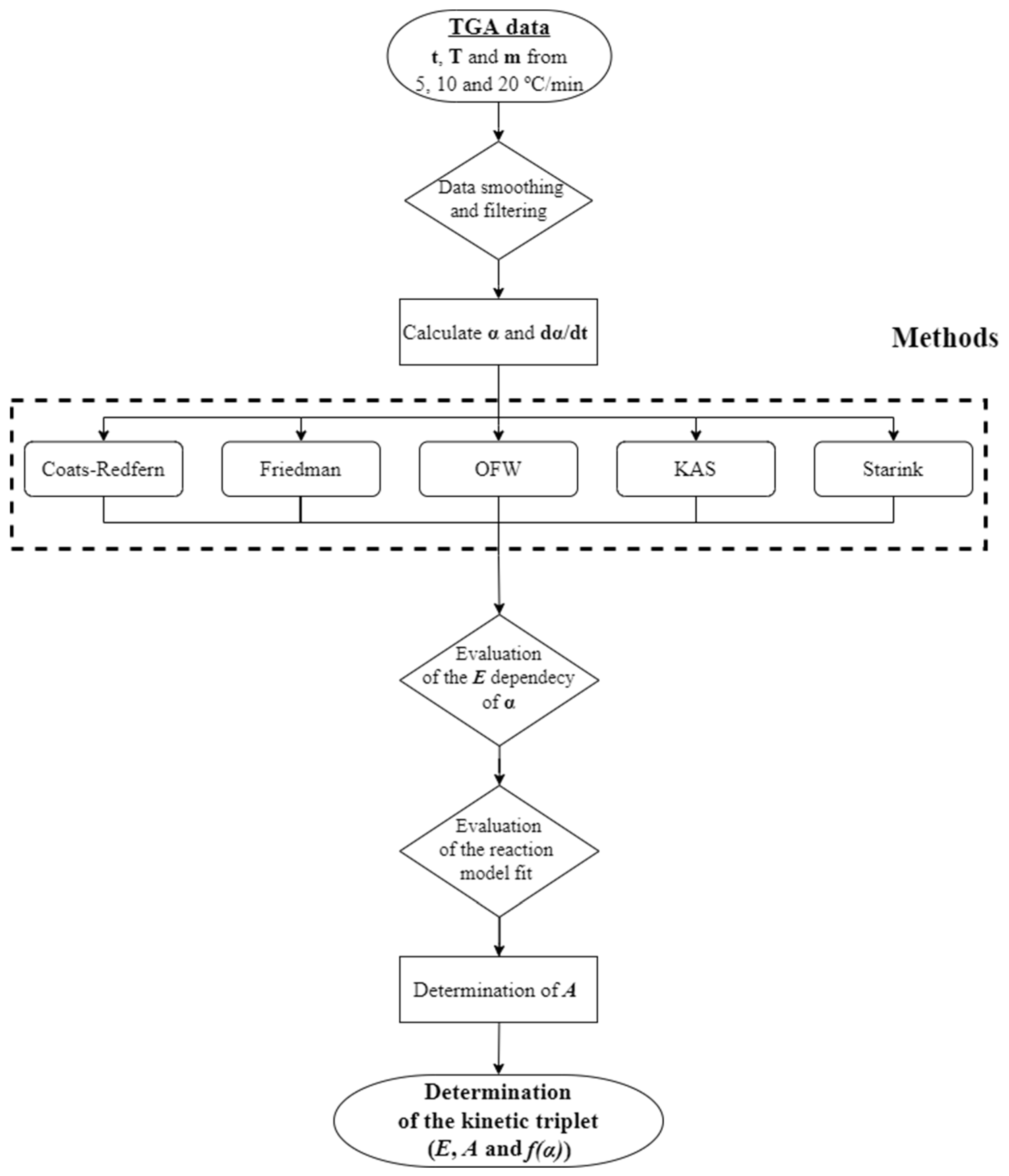
The thermal-conversion behavior of solid biomass fuels was analyzed using a piece of equipment from TA Instruments, model SDT 2960, in non-isothermal conditions up to a maximum temperature of 900 °C within three different regions. The first period of in-situ drying was performed to ensure the complete dehydration of the samples. For this, a heating ramp at 10 °C/min from the ambient temperature up to 105 °C was applied, followed by an isothermal stabilization period of 20 min. Then, a dynamic heating run was carried out with a steady heating rate from 105 to 900 °C.
Nevertheless, preliminary experiments were developed to guarantee that biomass combustion is only temperature-dependent, neglecting transport effects, and, therefore, the experiments were performed according to a pure kinetic regime [10,29]. Achieving this requires careful control of parameters such as particle size, initial mass, and airflow rate. Hence, a parametric analysis was initially developed to understand the influence of the atmosphere, its flow rate, the particle size, and also to evaluate the heating rate [10,29].
These were essential experiments to specify the proper conditions for the development of further thermogravimetric experiments. Furthermore, a strategy was implemented to avoid the differences in the conversion process due to the different moisture contents of the samples, by introducing an initial drying stage. Moreover, blank experiments were carried out to understand the effect of the gas-density variation in the weight measurement, commonly denominated as the buoyancy effect. Although the variation of the weight measurement can be reduced, it is essential to quantify it since the experiments are performed with a small amount of biomass.
Thus, based on the previous experiments, the TGA experiments were developed with particles with a size between 0.125 and 0.25 mm, an initial weight of 10 mg, and an air flow rate of 100 mL/min. (oxidant atmosphere). Additionally, heating rates of 5, 10, 20, and 100 °C/min up to 900 °C were considered after the drying stage. Before each experiment, the samples were measured on a high-accuracy scale (precision of 0.0001 g) and spread adequately in a 90 μL Alumina crucible used in the TG equipment to avoid diffusion problems.

2.3. Kinetic Study

The kinetic parameters for the eight fuels were determined based on the data generated from the TGA with the low heating rates, 5, 10, and 20 °C/min. This range of low heating rates was selected to balance experimental feasibility with practical relevance, enabling the resolution of overlapping thermal events and, consequently, improving the accuracy of kinetic-parameter estimation.
The fundamental basis of the kinetic models assumes that the solid-state transformation rate from biomass to volatile products, is generally described by Equation (1):
d α d t = k f ( α )
where t is the time, f ( α ) is a function called the reaction model which describes the dependence of the reaction model with the conversion rate (α), and k is the thermal dependence term that can be defined by the following Arrhenius Equation (2):
k = A exp E R T
Here E is the activation energy (J/mol), T is the absolute temperature (K), R is the universal gas constant (J/mol·K), and A is the pre-exponential factor (s−1). The former parameter is the minimum energy barrier required to break the bonds and change the chemical structure to another, while A is based on the collision theory and represents the number of collisions per unit of time occurring in the reaction.
Regarding the conversion rate, this term can be defined as a relation between the initial ( m 0 ), final ( m f ), and instantaneous ( m t ) sample mass. It can be obtained from each thermogravimetric experiment, and it is defined by Equation (3):
α = m 0 m t m 0 m f
For non-isothermal experiments, at a constant heating rate β = d T / d t , Equation (1) can be expressed as a function of temperature at a constant heating rate, yielding Equation (4):
d α d T = k f ( α ) 1 β
The experimental conditions and the reaction stage are considered to influence the reaction model. Generally, it is considered to be a first-order reaction, and this function can be expressed as ( 1 α ) [15,30]. Other functions commonly used are presented by White et al. [14]. After all these considerations, Equation (4) can be simplified as
d α 1 α = A β exp E R T d T
The left side of Equation (5) is a function of the conversion rate, and the right side is a function of the temperature. Integrating both sides of Equation (5), the following equation is obtained:
g α = 0 α d α ( 1 α ) = A β T 0 T exp E R T d T
Equation (6) has no exact solution, and it is necessary to use one of the two main mathematical approaches to solve this equation: (1) model-free methods (isoconversional) and (2) model-based methods [7]. Both methods are considered to provide a comprehensive kinetic analysis of the biomass combustion process and to obtain a better understanding of the complex and multi-step nature of biomass thermal degradation.
There are many isoconversional kinetic methods, and in this study, Friedman (FR) [31], Ozawa-Flynn-Wall (OFW) [32,33], Kissinger-Akahira-Sunose (KAS) [34,35,36], and Starink [37] are considered.
In model-fitting, Coats-Redfern (CR) [38], the most common model, was selected. This model can be fitted to experimental data, resulting in different reaction models that give the best statistical fit to evaluate the kinetic parameters. The CR model uses the asymptotic series expansion for approximating the exponential integral in Equation (6). According to this model, the kinetic parameters can be determined by the equation presented in Table 2 and by neglecting the term 2RT/E, which can be considered much lower than one. The value of A is then determined from the interception of the plot indicated in Table 2 [10], with the possibility of making this analysis at different stages of the conversion process. Otherwise, to complete the determination of the kinetic parameters A and f (α), usually, the Kissinger or compensation factor methods and master plots methods have been used to obtain both parameters, respectively [39]. The corresponding equations for each model and the advantages and disadvantages of their application can be found in Table 2.

2.4. Data Analysis

There is a significant amount of data either generated during the experiments or derived from their results. The TG and DTG curves from the TGA experiments allow the identification of different key parameters and indexes. On this basis, the analysis consists of identifying the ignition, peak, and burnout temperature and the maximum, average, and mass-loss rate in the different stages of biomass conversion, as well as the characteristic times when the biomass is ignited and completely oxidized. Furthermore, to assess the combustion performance of the different biomass samples, considering the previous parameters, four indexes can be calculated according to formulas presented by Yu et al. [41]. Hence, indexes for each stage of the biomass conversion, i.e., for ignition, volatile matter release, burnout, and an overall index, were calculated. All this information enables the thermal decomposition characterization of the different fuels. Table 3 presents all the parameters considered for the characterization of the TGA experiments and a brief description of the meaning of each one.
The kinetic parameters were directly obtained from the TGA experiments. Computational tools to derive this information are convenient, more accessible, and faster to handle, which is better for the large number of data acquired during the experiments. In the present study, a code using MATLAB 2020b was developed with mathematical and inbuilt functions to effortlessly smooth, filter, and fit the data. Figure 1 presents the main steps involved in determining the kinetic triplet parameters using different isoconversional methods and the CR equation.
This set of stages is fundamental to obtaining the effective kinetic parameters for the combustion of the selected fuels [42]. After each experiment, there were more than 3000 data points, and due to the sensitivity of the devices, it is expected that some noise is present in the data. The noise causes a discontinuity in the normal trend of the data and, consequently, leads to mathematical problems in the differentiation. Additionally, during the heating of the biomass sample, there was an amount of water and volatiles that were released, and a decrease in mass with time was expected. Hence, these points were removed, as well as the initial mass loss due to the drying of the fuel, where the weight loss data before 150 °C was not considered. The noise problem was resolved using a local regression applying a weighted linear least square method that smooths the data points and avoids inflection points in the mass-loss curve. Subsequently, the conversion values and their numerical differentiation were easily computed in MATLAB, and the number of data points was reduced according to the ICTAC recommendations [17]. Then, the kinetic parameters were determined by the slope of the numerical plots, which were obtained by the different methods through an inbuilt function for linear fitting.
The particular importance for post-processing TGA data is also highlighted by the utilization of the FR method. This method is different from the other isoconversional methods since it is based on the differential form of the Arrhenius equation, Equation (5), for the kinetic analysis. In this way, since no approximations or assumptions are used to solve the equation, it is considered more accurate than the other isoconversional methods which are known as integral methods [40]. However, Mishra et al. [43] compared the E values from different isoconversional methods, and it was observed that there were higher values at the end of the conversion from the FR method. This means that the FR method is more dependent on the instantaneous conversion rate and more prone to experimental noise. This statement is in line with the findings reported by Starink [44].

3. Results and Discussion

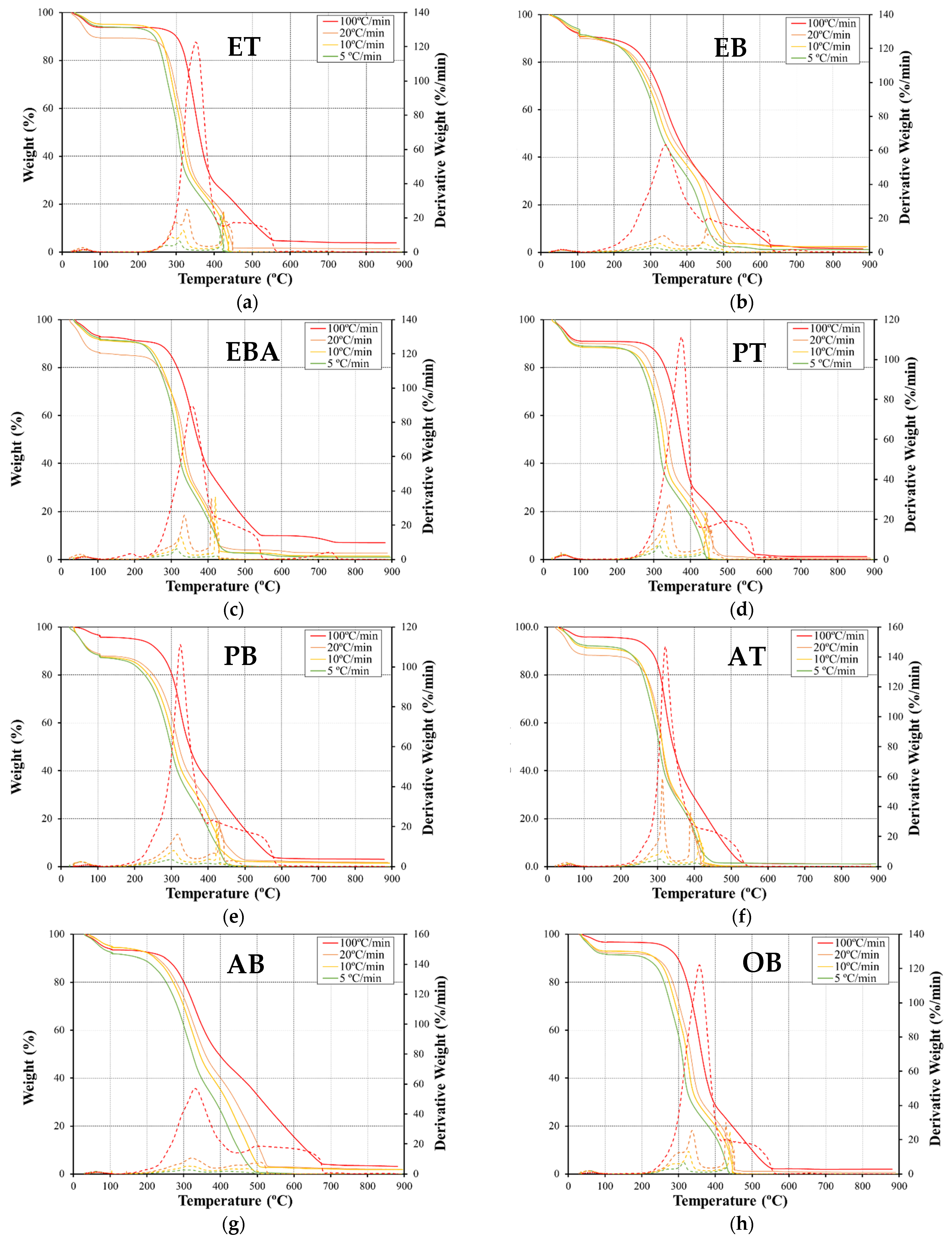
3.1. Thermal Decomposition

The evaluation of combustion performance at the particle scale is important for understanding the phenomena and acquiring accurate data to determine the kinetics of the different reactions. Since the heating rate is one of the significant factors in thermal decomposition, its influence was firstly analyzed. Then, the differences between each type of fuel and their different parts were analyzed to further understand the conversion of these types of solid fuels. During each thermogravimetric experiment, the values of the temperature (°C) and weight of the sample (mg) were registered at a 1 Hz rate.

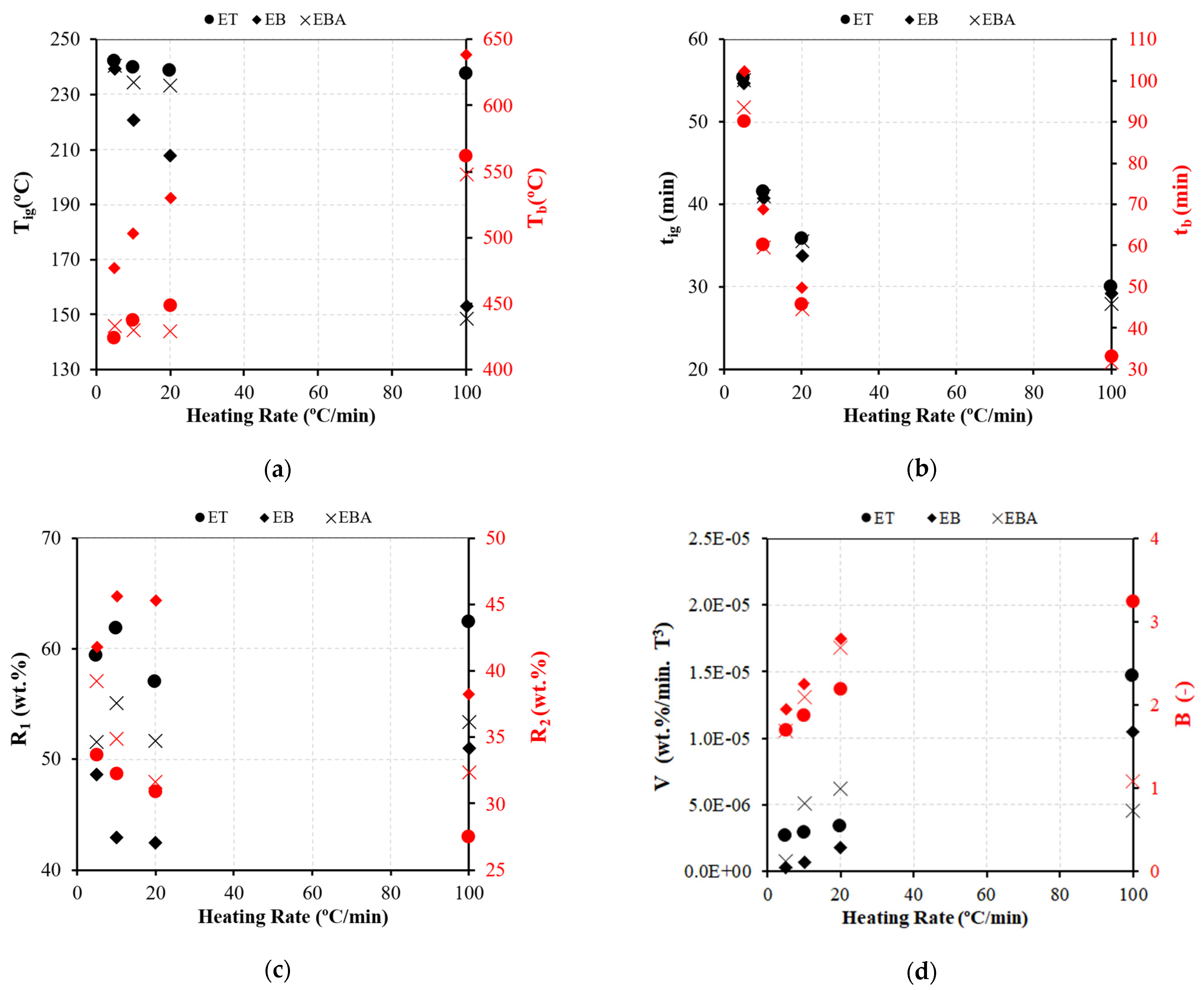
3.1.1. Influence of the Heating Rate

Figure 2 presents, for each fuel, the influence of the heating rate on the variation of the normalized weight loss by the thermogravimetric (TG) curve and shows the first derivative of the TG curve—known as the derivative thermogravimetric (DTG) curve—representing the rate of the weight-loss profile. The dashed lines represent the DTG curves while the solid lines correspond to the TG profiles. Looking at the different TG and DTG profiles, the conversion of all biomass fuels takes place over a wide range of temperatures and can be divided into three different zones. The first one is related to the drying stage, which during the experiments was performed at 105 °C for 20 min, mainly to ensure that a large amount of moisture was removed from the sample.
The present results are in agreement with previous studies reported in the literature [5,39,45,46,47,48]. However, some of these studies address biomass conversion in an inert atmosphere, and differ particularly in the last conversion stage due to the presence of oxygen that enhances the conversion of the solid residue by at least 15% [10]. Mishra et al. [5] also described an effect of an increase of the peak temperature of around 30 °C for pine, and more than 1% of volatile matter was released when the heating rates of 5 and 20 °C/min were compared. Siddiqi et al. [39] also described the same findings for waste biomass pyrolysis. Moreover, Álvarez et al. [46] studied the combustion of twenty-eight biomass samples using four different heating rates, and it was found that the temperature at maximum DTG of the second stage can occur at lower values, while the last stage can occur up to 627 °C.
Thus, the different characteristic parameters like Tig, Tb, T1, and T2, or mb are a function of the heating rate at which the particle is exposed. Considering the results from the present work, for instance, Tig was seen to have increased from 4 °C up to around 90 °C when the TG results from lower and higher heating rates were compared. tb was also substantially reduced as the heating rate was increased, achieving values three times lower than those at 5 °C/min. Figure 3 presents an example of the variation of these characteristic parameters, which are not directly observed in the TG and DTG curves Tmax, T1, and T2, for the different parts of eucalyptus fuel. Through these data, it is possible to observe that Tig, tig, and tb decreased as the heating rate increased, while the opposite effect was observed for Tb. These findings support the previously mentioned findings, where the higher heating rates were responsible for shifting the TG and DTG profile towards higher combustion temperatures.
However, R1 and R2 do not present a clear influence on the heating rate. Nonetheless, if the small fluctuations observed at intermediate heating rates are neglected, the heating rate has an inverse effect on both parameters. As already verified, the weight loss during devolatilization, R1, tends to increase up to 3%, while the weight loss during the char conversion, R2, tends to decrease, in particular for EBA, which showed a reduction of 7%. Regarding the volatile matter release (V) and burnout (B) performance indexes, they present a strong correlation with the heating rate since the second and third stages were substantially affected by this parameter. All characteristic parameters for every fuel, at different heating rates, are summarized in Table A1 in Appendix A.
Looking at the patterns of the TG and DTG curves for the different fuels, and their characteristic parameters, there are significant differences between the three samples of eucalyptus. For the inner part of the eucalyptus, the trunk sample, a higher mass loss was observed, as well as a more effective conversion of the second reaction.
Consequently, the combustion of ET is more reactive. According to Vega et al. [23], the thermal conversion of the inner part of biomass fuels is more evident due to their rich cellulosic structure, whereas the outer part is rich in lignin. This is why EBA and EB fuels present a higher conversion of char. EBA conversion in the last region still differs from the other fuels’ conversion as it presents a small peak at lower and higher temperatures, around 180 °C and 725 °C, respectively. A reduced amount of other constituents, like extractives, may be responsible for these variations [14,48].

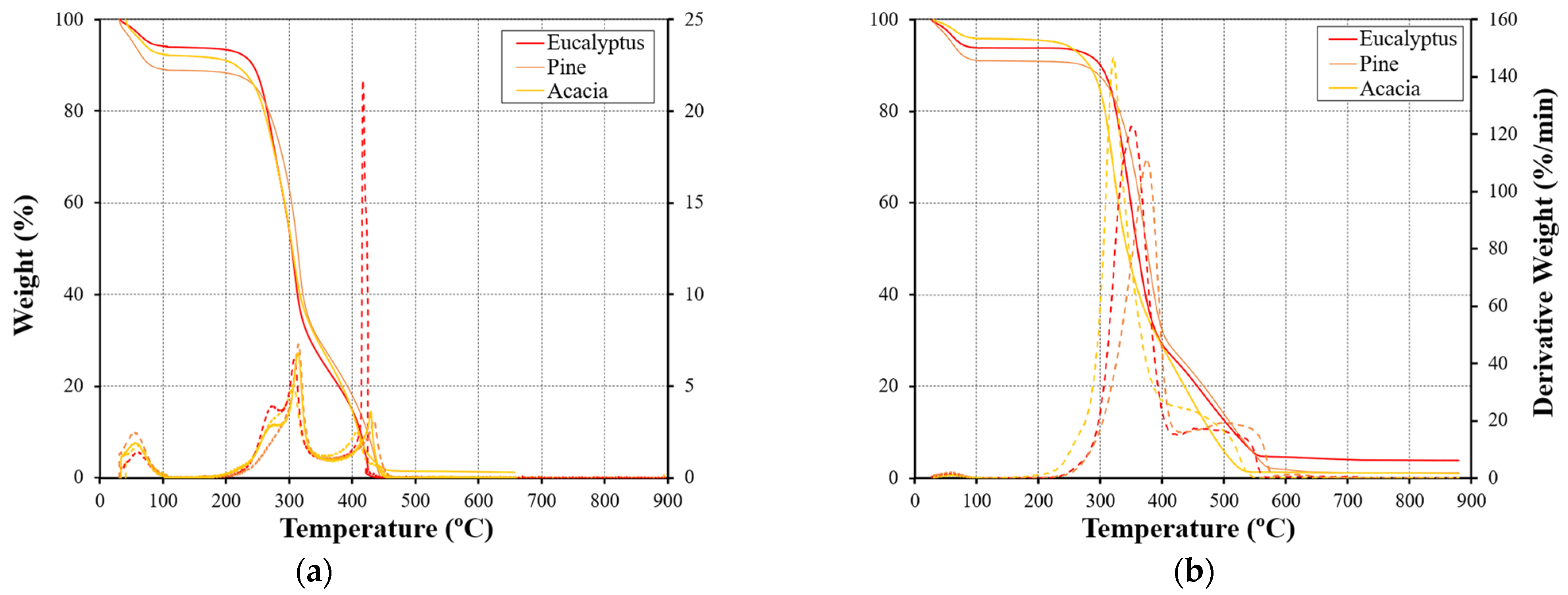
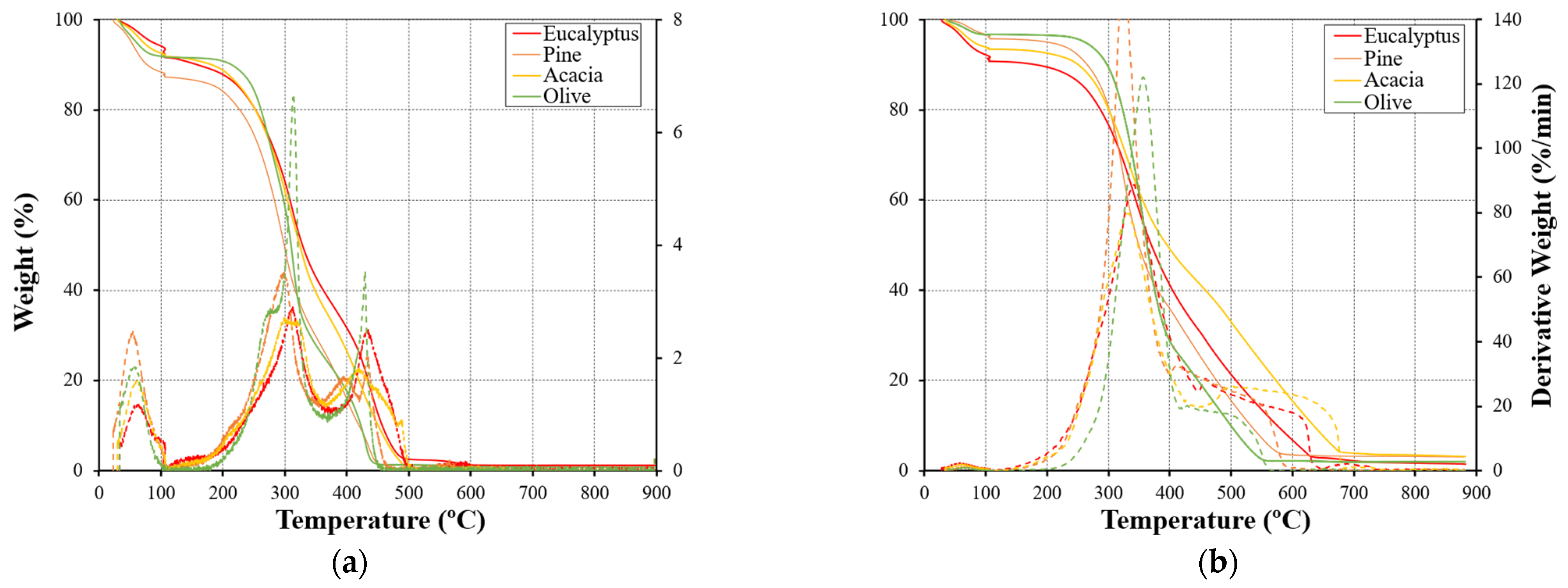
3.1.2. Comparative Analysis of Various Fuel Types

As previously referred to, there are significant differences in the thermal conversion behavior of all different fuels considered in this work. Also, differences are observed between their different parts. It is evident that the discrepancies are related to the intrinsic variability in the chemical and physical composition as well as in the structures and their thermal stability. The different contents of hemicellulose, cellulose, and lignin are important to justify the differences observed with the TG and DTG curves. For instance, the differences in residual weight at the end of the TGA experiments could be justified by the various contents of lignin, which are also dependent on the fixed carbon content of the samples. Figure 4 presents the conversion of the biomass samples from the trunk part of the different fuels (ET, PT, and AT), for the lowest and highest heating rates. As demonstrated in [28], AT has the highest fixed carbon content and at lower heating rates this was the fuel with the highest residual weight. However, at higher heating rates AT presented the lower mb since the char conversion increased, as opposed to the behavior presented by the other fuels. Furthermore, it is important to point out that the ET conversion in the third stage presents a high reactivity since there is a higher mass-loss rate identified by a slender peak in the DTG thermogram. This feature is observed for lower heating rates, although the differences between the fuels in this region are not significant at a higher heating rate.
In contrast, differences in the second stage can be observed. This is another important aspect that should be mentioned as DTG thermograms present large variations. At 5 °C/min the hemicellulose and cellulose, which should be converted in the range of temperatures of the second zone, are converted at different temperatures, while for higher heating rates their degradation overlaps and only one peak is visible. The results presented in Figure 4a suggest that hemicellulose reacts at lower temperatures, and the cellulose conversion occurs at a slightly higher temperature [14]. Moreover, the differences between the three fuels could be explained by looking at the volatile matter, although the cellulose content in these samples is another important factor that affects the maximum weight-loss rate. Figure 5 compares the weight loss from the branch part (EB, PB, AB, and OB) of the four biomass samples.
For these fuels, there is no separation of the hemicellulose and cellulose conversion in the second stage and the reactivity is lower than in the trunk samples. However, in the third zone, a higher mass-loss rate was observed as well as a degradation over a wider range of temperatures. Figure 6 presents a comparison of the characteristic parameters for the different fuels. In agreement with the previous discussion, there are differences between the fuels. The OB fuel shows a higher Tig but has the highest value of V since it is the fuel with higher R1. Regarding the performance in the last stage, EB presents higher R2 and B for lower heating rates, while at 100 °C/min PB degradation presented higher values. As demonstrated before for the eucalyptus samples, tig and tb present the same trend but the differences are reduced when the four fuels are compared, in particular at higher heating rates. This indicates that thermal conversion is more dependent on the heating rate than the fuel type.

3.2. Kinetic Parameters

E was calculated using four different isoconversional methods, OFW, FR, KAS, and the Starink method. Although the overall reaction mechanism with a single first-order reaction model is simpler to implement in a Computational Fluid Dynamics (CFD) model, biomass conversion has distinct reactions that need to be considered. The thermal oxidation of biomass is a complex process involving a set of physical processes and chemical reactions and a single reaction cannot correctly determine the kinetic parameters of biomass combustion. Consequently, the kinetic analysis relies on a two-step consecutive reaction model, which is composed of the two essential single reactions that more realistic describe the biomass combustion. The reaction scheme is hypothesized by Equations (7) and (8):
Biomass   k 1 Gases + Char
Char   k 2 Gases + Residue
Hence, the two main conversion processes, dealing with the devolatilization and char oxidation, are modeled.

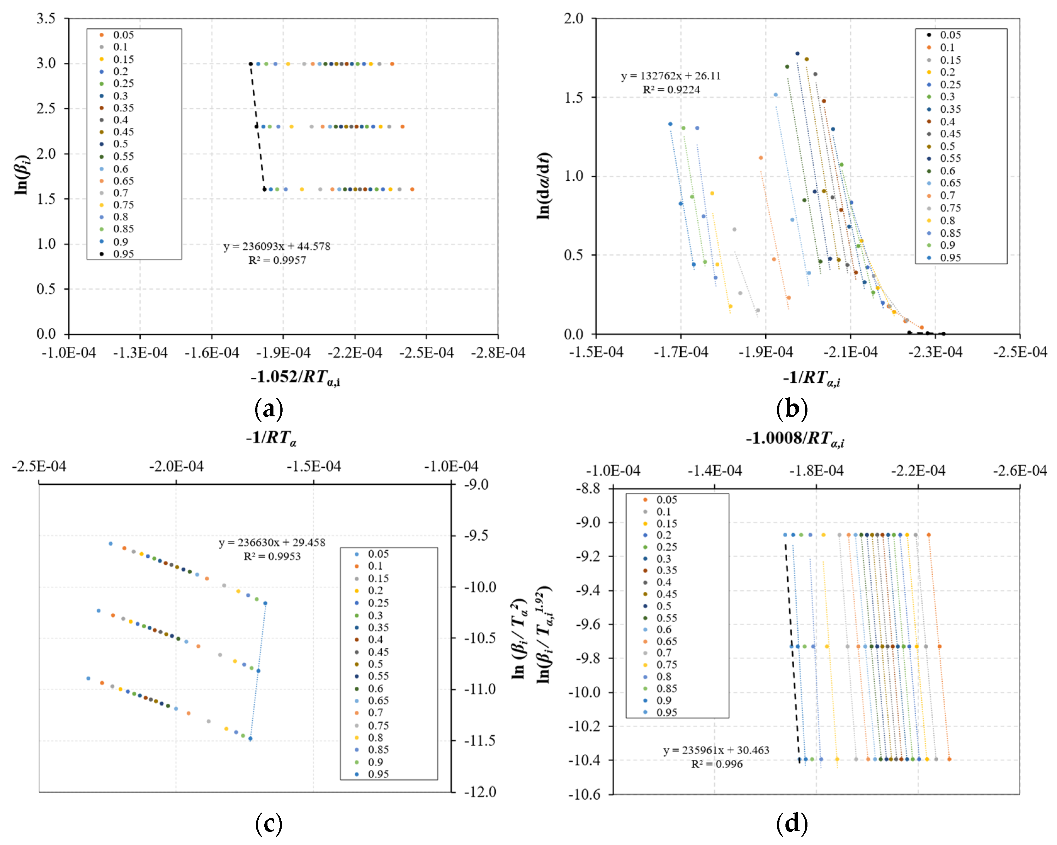
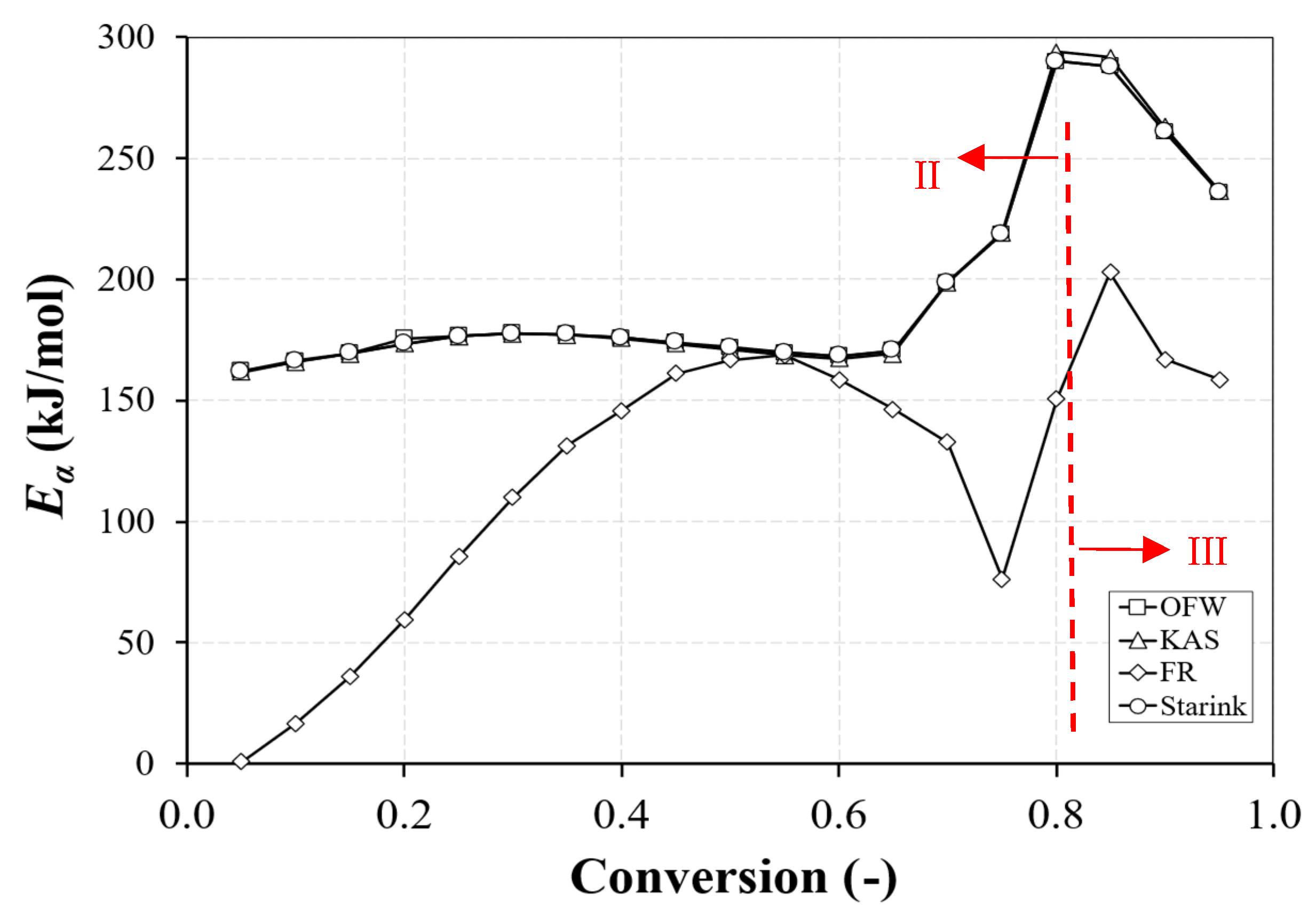
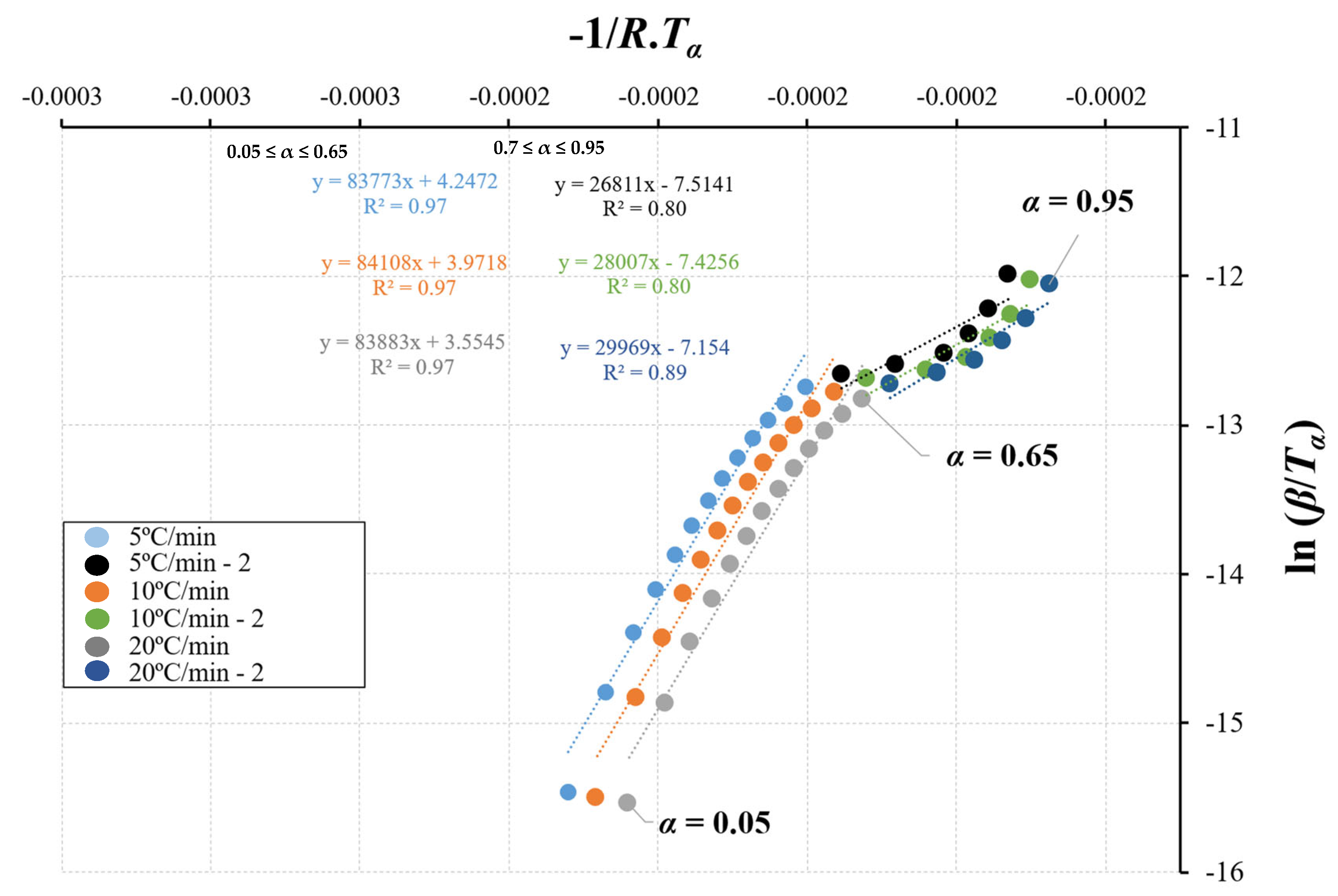
3.2.1. Evaluation of the Kinetic Method

The E calculated for all isoconversional methods considered in this work was obtained by linear regression, as indicated in Table 2. The plot of different terms enabled the determination of E for a conversion range between 5% and 95%, using a step size of 5%, as recommended by ICTAC [17]. Figure 7 presents the plots using the different specifications of the four kinetic methods, and the corresponding E was determined for each conversion by the linear equation [17].
Figure 8 presents an example of the results for E as a function of the conversion for the ET sample. It can be observed that the OFW, KAS, and Starink methods yield similar results, while, when using the FR method, the results are distinct. The first three methods are based on an integral form and, although there are some approximations associated with the temperature function, the results are similar. However, the FR method is based on the differential form of the conversion equation, without assumptions to assess the temperature function. Consequently, this method is sensitive to the experimental results with noise and zones where the reaction starts spontaneously, and it is known to be more susceptible to inconsistent results [40]. However, the plot for E is useful for understanding the nature of the decomposition reaction and for defining zones where the different reaction takes place. Table 4 presents the average E values considering the two main reactions during biomass combustion.
Nevertheless, the dependence of E on conversion is an indication that this is made up of independent and consecutive reactions. This is expected since biomass is composed of different components that decompose in different temperature ranges. Hence, since E varies significantly with conversion, isoconversional methods are not recommended [17]. This is because isoconversional methods assume that E remains constant throughout the entire biomass conversion process, which can lead to systematic errors [14]. To overcome this limitation, the CR method has been successfully applied to determine the kinetic parameters [12,15,20,46,49,50,51,52]. Hence, subsequently, the fitting of the CR method was evaluated using four types of simple reaction models, the 1st and 2nd order reaction models and the 1D and 2D diffusion models. Figure 9 presents an example of the linear regression curves, applying the separation based on the two different conversion stages of biomass combustion, which present 65% of conversion. In Table A2 (Appendix A), it is possible to verify the reaction mechanism selected to fit the conversion of each fuel and the corresponding kinetic parameters obtained through the linear regression equations. The linear correlation coefficient was higher than 0.906, representing a reasonable and acceptable data fit for all biomass fuels considered in this study.

3.2.2. Influence of the Type of Fuel

Taking into account that E means the minimum quantity of energy required to initiate chemical reactions, lower values correspond to higher reactivity. According to the kinetic data presented in Table A2 (Appendix A), the biomass fuels can be ranked by their reactivity in the devolatilization conversion process as EB > AB > PB > EBA > AT > OB > PT > ET. The values vary between 47.92 and 101.30 kJ/mol while, for char oxidation, E ranges from 14.97 to 35.48 kJ/mol. The devolatilization conversion was best characterized by reaction kinetics, using a second-order reaction model, and the char oxidation was successfully described by a diffusion-controlled mechanism. The diffusion of oxygen to char affects the combustion process and should be considered the main mechanism of thermal conversion of biomass in the last stage. The significant difference between E for the two stages is due to the lower values of E for lignin conversion when compared to cellulose degradation [46]; less energy is required to break the chemical bonds in lignin. Additionally, as there are different thermal conversion behaviors in the last stage of biomass combustion, the reactivity for this stage is defined as: ET > OB > PT > PB > AB> AT > EB > EBA.
Hence, the fuel type presented a significant influence on the activation energy during biomass combustion. Regarding the effect of the heating rate, the dependence of E with the heating rate was less evident and not all fuels presented a consistent trend with the heating rate. According to the literature, Magalhães et al. [15] analyzed the effect of the heating rate on the kinetic behavior, and a marginal difference was also reported. Álvarez et al. [46] studied the kinetic behavior of different biomass fuels including eucalyptus, olive, and pine, and similar results were observed. In this study, olive fuel also presented a lower reactivity. Fang et al. [49] and Shen et al. [51] determined E for pine combustion using a two-stage mechanism and CR method. Both studies presented lower energy requirements for char oxidation. Thus, the results from the present study are in the range of the reported results in the literature, although a small variation was detected, which can be attributed to the different physiochemical compositions of the biomass fuels.
Regarding the pre-exponential factor, another observation should be highlighted since the A parameter presented a dependence on the heating rate. As the heating rate increased, A also increased. As suggested by Siddiqi et al. [39] this behavior represents the increase in frequency and intensity of collisions among the molecules.

3.3. Reconstruction and Modeling

Based on the E and A data determined for the second and third stage, the conversion rate α can be predicted based on Equations (9) and (10) or (11), respectively.
Biomass   k 1 Gases + Char d α 1 d t = 1 β A 1 exp E 1 R T 1 α 2
Char   k 2 Gases + Residue d α 2 d t = 1 β A 2 exp E 2 R T 1 2 α
Char   k 2 Gases + Residue d α 2 d t = 1 β A 2 exp E 2 R T ln ( 1 α ) 1
Two possibilities were considered for the third reaction stage since the best fit to predict the conversion of EBA fuel differs from the other fuels. Hence, the char conversion was computed considering the 2D diffusion mechanism for EBA fuel (Equation (11)), while for the other fuels the conversion was predicted by using the 1D diffusion mechanism (Equation (10)).
Figure 10 illustrates the reconstruction and modeling of conversion as a function of temperature for the heating rates 5, 10, and 20 °C/min using parameters derived from the CR method. There are differences, in particular, at the initial stages of the conversion, and mainly for trunk samples (ET, PT, and AT). The differences are due to the hemicellulose and cellulose degradation at different temperatures in the second stage, and the average E for the second stage had some difficulties with reproducing the experimental behavior. The difference between the experimental and computed curves is a measure of the applicability of the derived kinetic parameters. To facilitate the comparison of the data, the square of the Pearson product moment correlation coefficient through the experimental and calculated values was determined for each fuel and heating rate. This value is interpreted as the proportion of the variance in the experimental results attributable to the variance in the results. A value above 0.95 was obtained, which corresponds to a good correlation between the experimental and numerical results. Therefore, the differences may be considered acceptable from the perspective of engineering calculations and predictions.

4. Conclusions

This paper presents a comprehensive analysis of the thermal decomposition and kinetics of various forest biomass fuels. The combustion behavior for the scales and conditions relevant to the operation in an industrial environment was analyzed, while a two-step reaction mechanism was used to describe the reaction kinetics. The main conclusions can be summarized as follows:
  • The evaluation of combustion performance at a particle scale by TGA showed that the conversion of all biomass fuels takes place over a wide range of temperatures, which can be divided into three different zones: drying, devolatilization, and char combustion;
  • Regarding the differences between the combustion behavior of the different fuels, a higher mass was observed for the inner part of the fuels, and there was a more effective conversion of the second-stage reaction. In its turn, the outer part of the eucalyptus presents a higher conversion of char, which may be associated with the higher lignin content of this fuel. Thus, variations in the chemical and physical composition, as well as in the structures and their thermal stability, justify the differences between the TG and DTG curves;
  • Based on the TGA data, a kinetic analysis was performed, which relied on a two-step consecutive reaction model. The utilization of isoconversional methods proved ineffective in determining the kinetic parameters since E is not constant throughout the particle conversion. The CR method was successfully applied to determine the kinetic parameters to overcome this limitation;
  • The devolatilization conversion was best characterized by the reaction kinetics model, using a second-order model, and the char oxidation was successfully described by a diffusion-controlled mechanism. The oxygen diffusion to the char affects the combustion process and should be considered the main mechanism of thermal conversion of biomass in the last stage;
  • The kinetic parameters during biomass combustion are strongly dependent on the type of fuel, while the effect of the heating rate was less evident, and not all fuels presented a consistent trend with the heating rate. According to the results, during the main conversion stage, devolatilization, the branch part of the fuels presented a lower energy of activation, while eucalyptus was the most reactive fuel.
Although the experiments were conducted on a laboratory scale, they provided valuable insights into transport phenomena at the particle level. The comparative analysis of kinetic modeling methods offers a novel contribution to the field. These findings can significantly support the scientific community by informing the development of more accurate CFD models, where the derived kinetic parameters enable the detailed prediction of particle mass loss and its integration with gas-phase reactions. Future work should explore the application of these parameters in larger-scale equipment and validate the models under real combustion conditions.

Author Contributions

Conceptualization, J.P.S., S.T. and J.C.T.; Methodology, J.P.S., S.T. and J.C.T.; Investigation, J.P.S.; Writing—Original Draft Preparation, J.P.S., J.C.T. and S.T.; Writing—Review and Editing, J.P.S., J.C.T. and S.T.; Supervision, J.C.T. and S.T. All authors have read and agreed to the published version of the manuscript.

Funding

This research was funded by Portuguese Foundation for Science and Technology (FCT) grant number SFRH/BD/130588/2017.

Data Availability Statement

Data is contained within the article.

Acknowledgments

The first author would like to express his acknowledgment for the support given by the Portuguese Foundation for Science and Technology (FCT) through the PhD grant SFRH/BD/130588/2017. FCT has supported this work within the R&D Units Project Scope UIDB/00319/2020 (ALGORITMI) and R&D Units Project Scope UIDP/04077/2020 (MEtRICs).

Conflicts of Interest

The authors declare no conflicts of interest.

Nomenclature

Latin symbols
APre-exponential factor, s−1
BBurnout performance, -
CComprehensive index, %/min2T3
EActivation energy, J/mol
IIgnition performance index, %/min3
kRate constant, s−1
mMass, kg
RUniversal Gas Contant, J/mol·K/Weight loss, %
tTime, s
TTemperature, °C
VVolatile matter release performance, %/T3
Greek symbols
α Extent of reaction, -
f α Reaction model, -
g α Integral form of the reaction model, -
β Heating rate, K/min
Subscripts and superscripts
0 Initial
i Instantaneous
b Burnout
List of Acronyms
ABAcacia Branch
ATAcacia Trunk
CRCoats-Redfern
DTGDerivative thermogravimetry
EBEucalyptus Branch
EBAEucalyptus Bark
ETEucalyptus Trunk
FRFriedman method
ICTACInternational Confederation for Thermal Analysis and Calorimetry
KASKissinger-Akahira-Sunose linear integral method
OBOlive Branch
PBPine Branch
PTPine Trunk
OFWOzawa-Flynn-Wall linear integral method

Appendix A

Table A1. Characteristic parameters obtained for different experiments.
Fuelβ
(°C/min)
TemperaturesMass LossTimeIndexes
T i g T b T 1 T 2 T max D T G m e a n D T G max R 1 R 2 m b t i g t b I V B C
ET5241.78423.96309.02416.42416.4221.200.5859.4133.640.15555.2890.014.26 × 10−32.64 × 10−61.704.97 × 10−7
10239.78436.98318.90423.89423.8923.011.1761.8032.250.14541.4460.039.25 × 10−32.87 × 10−61.881.07 × 10−6
20238.42448.47328.18423.93328.1824.932.1456.9830.920.18435.7545.591.53 × 10−23.33 × 10−62.192.09 × 10−6
100237.36561.91350.87451.07350.87122.719.9862.4527.480.48129.9532.931.24 × 10−11.47 × 10−53.243.87 × 10−5
EB5239.47476.82313.68435.70313.682.900.5748.6641.820.44854.68102.185.19 × 10−43.16 × 10−71.955.99 × 10−8
10220.59503.16321.57446.47446.475.641.1042.9745.590.45340.6568.842.02 × 10−36.36 × 10−72.262.53 × 10−7
20207.92530.03336.67451.63451.6314.572.1542.4845.300.39133.7149.728.69 × 10−31.81 × 10−62.801.37 × 10−6
100152.94638.04342.43457.31342.4363.399.9451.0438.280.29629.1133.576.49 × 10−21.05 × 10−54.224.22 × 10−5
EBA5240.55432.91315.18428.77315.186.210.5751.6239.230.49055.0693.411.21 × 10−37.21 × 10−71.691.41 × 10−7
10234.19429.65326.22419.17419.1736.341.1255.0734.860.31840.9059.401.50 × 10−25.12 × 10−62.101.72 × 10−6
20233.37428.77335.65408.17408.1735.472.0551.7131.660.53635.5444.622.24 × 10−26.25 × 10−62.693.11 × 10−6
100148.60547.86356.69726.63356.6989.779.5253.4132.400.91427.9531.541.02 × 10−14.58 × 10−61.087.06 × 10−5
PT5251.92445.11316.35436.46316.357.140.5551.8536.780.00757.2595.761.30 × 10−37.46 × 10−71.611.39 × 10−7
10247.39450.12328.17440.06440.0624.051.0954.6033.210.10243.2862.548.89 × 10−32.65 × 10−61.819.52 × 10−7
20242.06484.53339.58444.82339.5827.882.1957.1432.380.17535.1547.191.68 × 10−23.22 × 10−62.302.16 × 10−6
100240.67579.16374.80505.04374.80111.479.9861.9927.830.19229.6232.741.15 × 10−19.49 × 10−62.603.32 × 10−5
PB5232.17443.93298.05433.13298.053.460.5447.6138.960.2454.0996.296.64 × 10−43.70 × 10−71.577.60 × 10−8
10206.23461.45307.79423.42423.4222.611.0847.9438.070.3637.9963.459.38 × 10−33.08 × 10−62.211.06 × 10−6
20199.27494.73315.32430.09430.0923.032.1148.7737.450.2732.7047.491.48 × 10−23.19 × 10−62.571.69 × 10−6
100170.05589.39323.58411.21323.58111.1610.3154.5438.180.3128.7232.571.19 × 10−12.31 × 10−54.791.75 × 10−5
AT5238.62421.24308.75404.83308.755.080.5754.8336.220.5654.4690.781.03 × 10−37.18 × 10−71.901.20 × 10−7
10225.80424.92316.04411.38411.3820.681.1354.0736.950.2540.4659.008.66 × 10−33.04 × 10−62.091.08 × 10−6
20217.41417.51312.98389.47312.9858.082.1151.0936.140.1534.9344.183.76 × 10−21.12 × 10−52.626.22 × 10−6
100196.59539.53321.96457.54321.96146.9110.5058.4936.330.1029.2332.351.55 × 10−11.71 × 10−52.537.40 × 10−5
AB5236.71471.81304.35417.05304.352.710.5754.5037.740.4854.73101.624.87 × 10−43.34 × 10−72.095.89 × 10−8
10210.91505.79317.73511.51317.735.271.1557.1135.510.3037.5866.842.10 × 10−34.06 × 10−71.522.69 × 10−7
20200.77527.77321.61510.10321.6110.672.2757.1735.340.3233.1849.216.53 × 10−38.77 × 10−71.731.14 × 10−6
100165.86680.97332.70504.08332.7057.0010.0356.0934.190.3728.6333.385.96 × 10−26.03 × 10−63.013.05 × 10−5
OB5240.99437.76313.61429.19313.616.670.5758.1832.750.0255.3394.431.28 × 10−37.63 × 10−71.701.49 × 10−7
10229.04445.48327.79438.42438.4224.561.1560.0832.110.1140.2561.219.97 × 10−32.96 × 10−61.961.20 × 10−6
20224.65451.47336.07428.49428.4930.052.2460.3431.130.1834.4544.991.94 × 10−24.31 × 10−62.452.96 × 10−6
100218.13558.84354.60433.67354.60122.1310.5067.4827.250.1928.7031.781.34 × 10−12.00 × 10−54.314.82 × 10−5
Table A2. Reaction mechanism, linear regression, and kinetic parameters obtained through the CR method.
FuelReaction and Mechanismβ (°C/min)EquationR2E (kJ/mol)A (min−1)
ETDevolatilization/2nd order 5 y = 101295 x + 8.2521 0.992101.302.34 × 108
10 y = 101251 x + 7.8343 0.991101.253.08 × 108
20 y = 100489 x + 7.2413 0.990100.493.37 × 108
Char oxidation/1D diffusion 5 y = 15839 x 10.5 0.90815.840.26
10 y = 16605 x 10.452 0.90616.610.58
20 y = 17569 x 10.335 0.97317.571.37
EBDevolatilization/2nd order 5 y = 51765 x 2.7084 0.99751.772.07 × 103
10 y = 49487 x 3.414 0.99749.491.96 × 103
20 y = 47922 x 3.9658 0.99647.922.18 × 103
Char oxidation/1D diffusion 5 y = 29083 x 8.6433 0.98229.083.08
10 y = 31628 x 8.387 0.98531.638.67
20 y = 31225 x 8.6433 0.99431.2313.24
EBADevolatilization/2nd order 5 y = 85654 x + 4.5529 0.99885.654.89 × 106
10 y = 86200 x + 4.327 0.99986.207.85 × 106
20 y = 82918 x + 3.3558 0.99982.925.72 × 106
Char oxidation/2D diffusion 5 y = 30592 x 8.1818 0.98535.485.15
10 y = 30967 x 8.2068 0.99430.9710.16
20 y = 35476 x 7.4913 0.98535.4847.61
PTDevolatilization/2nd order 5 y = 98227 x + 7.0495 0.99498.236.81 × 107
10 y = 97665 x + 6.498 0.99697.677.80 × 107
20 y = 95716 x + 5.6669 0.99595.726.66 × 107
Char oxidation/1D diffusion 5 y = 21532 x 9.6393 0.96821.530.84
10 y = 24184 x 9.2627 0.94724.182.76
20 y = 20082 x 10.082 0.97120.082.02
PBDevolatilization/2nd order 5 y = 62339 x + 0.0238 0.99762.343.84 × 104
10 y = 63929 x + 0.1433 0.99763.938.87 × 104
20 y = 62681 x 0.4084 0.99762.671.00 × 105
Char oxidation/1D diffusion 5 y = 20051 x 9.8785 0.99820.050.62
10 y = 22106 x 9.5897 0.99622.111.82
20 y = 24687 x 9.2734 0.99124.695.58
ATDevolatilization/2nd order 5 y = 85995 x + 4.972 0.99685.997.46 × 106
10 y = 85790 x + 4.5696 0.99685.799.96 × 106
20 y = 85606 x + 4.185 0.99685.611.35 × 107
Char oxidation/1D diffusion 5 y = 19874 x 9.7866 0.98919.870.67
10 y = 24213 x 9.1003 0.99024.213.25
20 y = 29230 x 8.3163 0.96829.2317.19
ABDevolatilization/2nd order 5 y = 54053 x 2.1273 0.99954.053.87 × 103
10 y = 52172 x 2.7972 0.99852.173.83 × 103
ABDevolatilization/2nd order20 y = 49453 x 3.5741 0.99649.453.34 × 103
Char oxidation/1D diffusion 5 y = 22176 x 9.7457 0.99422.180.78
10 y = 24926 x 9.4639 0.99724.932.33
20 y = 24551 x 9.7265 0.99524.553.52
OBDevolatilization/2nd order 5 y = 87737 x + 5.2242 0.99987.749.80 × 106
10 y = 87342 x + 4.7329 0.99987.341.19 × 107
20 y = 86760 x + 4.2662 0.99886.761.49 × 107
Char oxidation/1D diffusion 5 y = 14977 x 10.721 0.97814.970.20
10 y = 15894 x 10.643 0.90615.890.46
20 y = 19990 x 9.9649 0.97819.992.26

References

  1. Saidur, R.; Abdelaziz, E.A.; Demirbas, A.; Hossain, M.S.; Mekhilef, S. A review on biomass as a fuel for boilers. Renew. Sustain. Energy Rev. 2011, 15, 2262–2289. [Google Scholar] [CrossRef]
  2. Nussbaumer, T. Combustion and Co-combustion of Biomass: Fundamentals, Technologies, and Primary Measures for Emission Reduction. Energy Fuels 2003, 17, 1510–1521. [Google Scholar] [CrossRef]
  3. Jones, J.M.; Lea-Langton, A.R.; Ma, L.; Pourkashanian, M.; Williams, A. Pollutants Generated by the Combustion of Solid Biomass Fuels; Springer: Berlin/Heidelberg, Germany, 2015. [Google Scholar] [CrossRef]
  4. Cai, J.; Xu, D.; Dong, Z.; Yu, X.; Yang, Y.; Banks, S.W.; Bridgwater, A.V. Processing thermogravimetric analysis data for isoconversional kinetic analysis of lignocellulosic biomass pyrolysis: Case study of corn stalk. Renew. Sustain. Energy Rev. 2018, 82, 2705–2715. [Google Scholar] [CrossRef]
  5. Mishra, R.K.; Mohanty, K. Pyrolysis kinetics and thermal behavior of waste sawdust biomass using thermogravimetric analysis. Bioresour. Technol. 2018, 251, 63–74. [Google Scholar] [CrossRef]
  6. Vyazovkin, S.; Wight, C.A. Isothermal and non-isothermal kinetics of thermally stimulated reactions of solids. Int. Rev. Phys. Chem. 1998, 17, 407–433. [Google Scholar] [CrossRef]
  7. Garcia-Maraver, A.; Perez-Jimenez, J.A.; Serrano-Bernardo, F.; Zamorano, M. Determination and comparison of combustion kinetics parameters of agricultural biomass from olive trees. Renew. Energy. 2015, 83, 897–904. [Google Scholar] [CrossRef]
  8. Saeed, M.A.; Andrews, G.E.; Phylaktou, H.N.; Gibbs, B.M. Global kinetics of the rate of volatile release from biomasses in comparison to coal. Fuel 2016, 181, 347–357. [Google Scholar] [CrossRef]
  9. Su, Y.; Luo, Y.; Wu, W.; Zhang, Y.; Zhao, S. Characteristics of pine wood oxidative pyrolysis: Degradation behavior, carbon oxide production and heat properties. J. Anal. Appl. Pyrolysis 2012, 98, 137–143. [Google Scholar] [CrossRef]
  10. Fraga, L.G.; Silva, J.; Teixeira, S.; Soares, D.; Ferreira, M.; Teixeira, J. Thermal Conversion of Pine Wood and Kinetic Analysis under Oxidative and Non-Oxidative Environments at Low Heating Rate. Proceedings 2020, 58, 23. [Google Scholar] [CrossRef]
  11. Anca-Couce, A.; Zobel, N.; Berger, A.; Behrendt, F. Smouldering of pine wood: Kinetics and reaction heats. Combust. Flame. 2012, 159, 1708–1719. [Google Scholar] [CrossRef]
  12. Shen, D.K.; Gu, S.; Jin, B.; Fang, M.X. Thermal degradation mechanisms of wood under inert and oxidative environments using DAEM methods. Bioresour. Technol. 2011, 102, 2047–2052. [Google Scholar] [CrossRef] [PubMed]
  13. Vyazovkin, S.; Chrissafis, K.; Di Lorenzo, M.L.; Koga, N.; Pijolat, M.; Roduit, B.; Sbirrazzuoli, N.; Suñol, J.J. ICTAC Kinetics Committee recommendations for collecting experimental thermal analysis data for kinetic computations. Thermochim. Acta 2014, 590, 1–23. [Google Scholar] [CrossRef]
  14. White, J.E.; Catallo, W.J.; Legendre, B.L. Biomass pyrolysis kinetics: A comparative critical review with relevant agricultural residue case studies. J. Anal. Appl. Pyrolysis 2011, 91, 1–33. [Google Scholar] [CrossRef]
  15. Magalhães, D.; Kazanç, F.; Riaza, J.; Erensoy, S.; Kabaklı, Ö.; Chalmers, H. Combustion of Turkish lignites and olive residue: Experiments and kinetic modelling. Fuel 2017, 203, 868–876. [Google Scholar] [CrossRef]
  16. Vyazovkin, S.; Sbirrazzuoli, N. Isoconversional Kinetic Analysis of Thermally Stimulated Processes in Polymers. Macromol. Rapid Commun. 2006, 27, 1515–1532. [Google Scholar] [CrossRef]
  17. Vyazovkin, S.; Burnham, A.K.; Criado, J.M.; Pérez-Maqueda, L.A.; Popescu, C.; Sbirrazzuoli, N. ICTAC Kinetics Committee recommendations for performing kinetic computations on thermal analysis data. Thermochim. Acta 2011, 520, 1–19. [Google Scholar] [CrossRef]
  18. Khawam, A.; Flanagan, D.R. Basics and Applications of Solid-State Kinetics: A Pharmaceutical Perspective. J. Pharm. Sci. 2006, 95, 472–498. [Google Scholar] [CrossRef]
  19. Rico, J.J.; Pérez-Orozco, R.; Vilas, D.P.; Porteiro, J. TG/DSC and kinetic parametrization of the combustion of agricultural and forestry residues. Biomass Bioenergy 2022, 162, 106485. [Google Scholar] [CrossRef]
  20. Xu, X.; Pan, R.; Chen, R. Combustion Characteristics, Kinetics, and Thermodynamics of Pine Wood Through Thermogravimetric Analysis. Appl. Biochem. Biotechnol. 2021, 193, 1427–1446. [Google Scholar] [CrossRef]
  21. Chen, R.; Li, Q.; Xu, X.; Zhang, D.; Hao, R. Combustion characteristics, kinetics and thermodynamics of Pinus Sylvestris pine needle via non-isothermal thermogravimetry coupled with model-free and model-fitting methods. Case Stud. Therm. Eng. 2020, 22, 100756. [Google Scholar] [CrossRef]
  22. Fu, S.; Chen, H.; Yang, J.; Yang, Z. Kinetics of thermal pyrolysis of Eucalyptus bark by using thermogravimetric-Fourier transform infrared spectrometry technique. J. Therm. Anal. Calorim. 2019, 139, 3527–3535. [Google Scholar] [CrossRef]
  23. Vega, L.Y.; López, L.; Valdés, C.F.; Chejne, F. Assessment of energy potential of wood industry wastes through thermochemical conversions. Waste Manag. 2019, 87, 108–118. [Google Scholar] [CrossRef] [PubMed]
  24. Cai, Z.; Ma, X.; Fang, S.; Yu, Z.; Lin, Y. Thermogravimetric analysis of the co-combustion of eucalyptus residues and paper mill sludge. Appl. Therm. Eng. 2016, 106, 938–943. [Google Scholar] [CrossRef]
  25. Silva, J.P.; Teixeira, S.; Grilo, É.; Peters, B.; Teixeira, J.C. Analysis and monitoring of the combustion performance in a biomass power plant. Clean. Eng. Technol. 2021, 5, 100334. [Google Scholar] [CrossRef]
  26. Ferreira, S.; Monteiro, E.; Brito, P.; Vilarinho, C. Biomass resources in Portugal: Current status and prospects. Renew. Sustain. Energy Rev. 2017, 78, 1221–1235. [Google Scholar] [CrossRef]
  27. Nunes, L.J.R.; Loureiro, L.M.E.F.; Sá, L.C.R.; Silva, H.F.C. Evaluation of the potential for energy recovery from olive oil industry waste: Thermochemical conversion technologies as fuel improvement methods. Fuel 2020, 279, 118536. [Google Scholar] [CrossRef]
  28. Silva, J.P.; Teixeira, S.; Teixeira, J.C. Characterization of the physicochemical and thermal properties of different forest residues. Biomass Bioenergy 2023, 175, 106870. [Google Scholar] [CrossRef]
  29. Fraga, L.G.; Silva, J.; Teixeira, S.; Soares, D.; Ferreira, M.; Teixeira, J. Influence of Operating Conditions on the Thermal Behavior and Kinetics of Pine Wood Particles using Thermogravimetric Analysis. Energies 2020, 13, 2756. [Google Scholar] [CrossRef]
  30. Bahng, M.-K.; Mukarakate, C.; Robichaud, D.J.; Nimlos, M.R. Current technologies for analysis of biomass thermochemical processing: A review. Anal. Chim. Acta. 2009, 651, 117–138. [Google Scholar] [CrossRef]
  31. Friedman, H.L. Kinetics of thermal degradation of char-forming plastics from thermogravimetry. Application to a phenolic plastic. J. Polym. Sci. Part C Polym. Symp. 1964, 6, 183–195. [Google Scholar] [CrossRef]
  32. Ozawa, T. A New Method of Analyzing Thermogravimetric Data. Bull. Chem. Soc. Jpn. 1965, 38, 1881–1886. [Google Scholar] [CrossRef]
  33. Flynn, J.H.; Wall, L.A. General treatment of the thermogravimetry of polymers. J. Res. Natl. Bur. Stand. Sect. A Phys. Chem. 1966, 70A, 487. [Google Scholar] [CrossRef]
  34. Kissinger, H. Variation of peak temperature with heating rate in differential thermal analysis. J. Res. Natl. Bur. Stand. 1956, 57, 217–221. [Google Scholar] [CrossRef]
  35. Kissinger, H.E. Reaction Kinetics in Differential Thermal Analysis. Anal. Chem. 1957, 29, 1702–1706. [Google Scholar] [CrossRef]
  36. Akahira, T.; Sunose, T. Method of determining activation deterioration constant of electrical insulating materials. Res. Rep. Chiba Inst. Technol. (Sci. Technol.) 1971, 16, 22–31. [Google Scholar]
  37. Starink, M. The determination of activation energy from linear heating rate experiments: A comparison of the accuracy of isoconversion methods. Thermochim. Acta 2003, 404, 163–176. [Google Scholar] [CrossRef]
  38. Coats, A.W.; Redfern, J.P. Kinetic Parameters from Thermogravimetric Data. Nature 1964, 201, 68–69. [Google Scholar] [CrossRef]
  39. Siddiqi, H.; Bal, M.; Kumari, U.; Meikap, B.C. In-depth physiochemical characterization and detailed thermo-kinetic study of biomass wastes to analyze its energy potential. Renew. Energy 2019, 148, 756–771. [Google Scholar] [CrossRef]
  40. Dhyani, V.; Bhaskar, T. Kinetic Analysis of Biomass Pyrolysis. In Waste Biorefinery; Elsevier: Amsterdam, The Netherlands, 2018; pp. 39–83. [Google Scholar] [CrossRef]
  41. Yu, D.; Chen, M.; Wei, Y.; Niu, S.; Xue, F. An assessment on co-combustion characteristics of Chinese lignite and eucalyptus bark with TG–MS technique. Powder Technol. 2016, 294, 463–471. [Google Scholar] [CrossRef]
  42. Conesa, J.A.; Marcilla, A.; Caballero, J.A.; Font, R. Comments on the validity and utility of the different methods for kinetic analysis of thermogravimetric data. J. Anal. Appl. Pyrolysis 2001, 58–59, 617–633. [Google Scholar] [CrossRef]
  43. Mishra, G.; Kumar, J.; Bhaskar, T. Kinetic studies on the pyrolysis of pinewood. Bioresour. Technol. 2015, 182, 282–288. [Google Scholar] [CrossRef]
  44. Starink, M.J. A new method for the derivation of activation energies from experiments performed at constant heating rate. Thermochim. Acta 1996, 288, 97–104. [Google Scholar] [CrossRef]
  45. Vamvuka, D.; Sfakiotakis, S. Combustion behaviour of biomass fuels and their blends with lignite. Thermochim. Acta 2011, 526, 192–199. [Google Scholar] [CrossRef]
  46. Álvarez, A.; Pizarro, C.; García, R.; Bueno, J.L.; Lavín, A.G. Determination of kinetic parameters for biomass combustion. Bioresour. Technol. 2016, 216, 36–43. [Google Scholar] [CrossRef]
  47. Chen, Z.; Zhu, Q.; Wang, X.; Xiao, B.; Liu, S. Pyrolysis behaviors and kinetic studies on Eucalyptus residues using thermogravimetric analysis. Energy Convers. Manag. 2015, 105, 251–259. [Google Scholar] [CrossRef]
  48. Sanchez-Silva, L.; López-González, D.; Villaseñor, J.; Sánchez, P.; Valverde, J.L. Thermogravimetric–mass spectrometric analysis of lignocellulosic and marine biomass pyrolysis. Bioresour. Technol. 2012, 109, 163–172. [Google Scholar] [CrossRef]
  49. Fang, X.; Jia, L.; Yin, L. A weighted average global process model based on two−stage kinetic scheme for biomass combustion. Biomass Bioenergy 2013, 48, 43–50. [Google Scholar] [CrossRef]
  50. Gil, M.V.; Casal, D.; Pevida, C.; Pis, J.J.; Rubiera, F. Thermal behaviour and kinetics of coal/biomass blends during co-combustion. Bioresour. Technol. 2010, 101, 5601–5608. [Google Scholar] [CrossRef]
  51. Shen, D.K.; Gu, S.; Luo, K.H.; Bridgwater, A.V.; Fang, M.X. Kinetic study on thermal decomposition of woods in oxidative environment. Fuel 2009, 88, 1024–1030. [Google Scholar] [CrossRef]
  52. Yorulmaz, S.Y.; Atimtay, A.T. Investigation of combustion kinetics of treated and untreated waste wood samples with thermogravimetric analysis. Fuel Process. Technol. 2009, 90, 939–946. [Google Scholar] [CrossRef]
Figure 1. Flowchart of the different stages considered in kinetic analysis.
Energies 18 03299 g001
Figure 2. TG and DTG curves of (a) ET, (b) EB, (c) EBA, (d) PT, (e) PB, (f) AT, (g) AB, and (h) OB.
Energies 18 03299 g002
Figure 3. Comparison of the different parts of eucalyptus fuel in terms of characteristic parameters: (a) ignition and burnout temperature, (b) ignition and burnout time, (c) weight loss during devolatilization and char combustion, and (d) indexes of volatile-matter release and burnout performance.
Energies 18 03299 g003
Figure 4. TG and DTG curves for the trunk part of the different samples at: (a) lower heating rate—5 °C/min, and (b) higher heating rate—100 °C/min.
Energies 18 03299 g004
Figure 5. TG and DTG curves for the branch part of the different samples at: (a) lower heating rate—5 °C/min, and (b) higher heating rate—100 °C/min.
Energies 18 03299 g005
Figure 6. Comparison of the different biomass fuels (from the same part of the tree—branches) in terms of characteristic parameters: (a) ignition and burnout temperature, (b) ignition and burnout time, (c) weight loss during devolatilization and char combustion, and (d) indexes of volatile matter release and burnout performance.
Energies 18 03299 g006
Figure 7. Curves obtained for the different methods: (a) OFW, (b) FR, (c) KAS, and (d) Starink for ET sample.
Energies 18 03299 g007
Figure 8. E value as a function of the conversion for ET. The red dashed line symbolizes the transition from the devolatilization (II) to the char oxidation (III) reaction during the combustion of biomass.
Energies 18 03299 g008
Figure 9. Curves obtained for CR method considering a first-order reaction and for ET sample.
Energies 18 03299 g009
Figure 10. Comparison between experimental and modeled conversion results for the different samples: (a) ET, (b) EB, (c) EBA, (d) PT, (e) PB, (f) AT, (g) AB, and (h) OB.
Energies 18 03299 g010
Table 1. Physicochemical properties and calorific value of the different biomass fuels [28].
PropertyParameterAcaciaEucalyptusPineOlive
TrunkBranchesBarkTrunk *BranchesTrunk *Branches
Proximate Analysis (%, db)Moisture5.06.23.42.16.711.511.2
Volatile matter81.877.889.688.982.983.781.5
Ashes1.10.74.21.03.20.81.8
Fixed Carbon17.121.56.210.113.915.516.7
Ultimate Analysis (%, db)Carbon45.4052.4043.1047.2055.9047.3049.40
Hydrogen6.887.386.467.037.556.406.95
Nitrogen0.773.210.250.111.440.130.24
Sulfur0.010.040.010.010.010.990.88
Oxygen46.9436.9750.1845.6535.1045.1842.53
Air–Fuel Ratio
(stoichiometric—gair/gsample)
5.546.945.005.857.485.696.23
Calorific Value (db)HHV (MJ/kg)17.1420.4115.2017.5622.3019.1017.71
LHV (MJ/kg)15.6618.8113.8116.0520.6718.6016.22
* without bark, db—dry basis.
Table 2. Different kinetics methods used in literature—equation and advantages and disadvantages. Adapted from [4,40].
MethodEquation Determination
(Slope of the Plots)
Advantages and Disadvantages
FR ln β i d α d T α , i = ln A α f ( α ) E α R T α , i ln β i d α d T α , i v s 1 R T α , i Simple and accurate; numerically unstable and sensitive to data noise
OFW ln β i = ln A α E α R g ( α ) 5.331 1.052 E α R T α , i ln β i v s 1.052 R T α , i Oversimplified temperature integral
KAS ln β i T α , i 2 = ln A α R E α g ( α ) E α R T α , i ln β i T α , i 2 v s 1 R T α , i More accurate than OFW;
oversimplified temperature integral
Starink ln β i T α , i 1.92 = Constant 1.008 E α R T α , i ln β i T α , i 1.92 v s 1.0008 R T α , i More accurate temperature integral approximation
CR ln g ( α ) T 2 = ln A R β E 1 2 R T E E R T ln g α T α 2 v s 1 R T α Forcible fitting to reaction mechanism; single values of E are obtained
Table 3. Characteristic parameters considered for thermal-analysis evaluation and comparison.
PropertyParameterDescription
Temperature T i g Ignition temperature (°C). Corresponds to the beginning of the weight loss and is defined as the temperature at which the rate of weight loss reaches 1%/min after the initial moisture loss peak in the DTG profile.
T b Burnout temperature (°C). It is identified when the last peak comes to the end and is the temperature at which the sample is completely oxidized. It is taken as the point immediately before the reaction ceases when the rate of weight loss is down to 1%/min.
T 1 Peak temperature in devolatilization (°C). It is the point at which the maximum reaction rate occurs during devolatilization.
T 2 Peak temperature in char combustion (°C). It is the point at which the maximum reaction rate occurs during char combustion.
T max Temperature at the maximum weight loss (°C). It is the point at which the maximum reaction rate occurs.
Mass Loss D T G m e a n Average weight loss rate, wt.%/min
D T G max Maximum weight loss rate, wt.%/min
R 1 Weight loss during devolatilization, wt.%
R 2 Weight loss during char combustion, wt.%
m b Residual weight, mg
Time t i g Ignition time, min.
t b Burnout time, min.
Indexes I = D T G max t b t i g It indicates the ignition performance. This means how fast or slow the fuel is ignited. wt.%/min3
V = D T G max T P T i g Δ T 1 / 2 Reflects the volatile matter release performance. wt.%/min.T3
B = Δ T b Δ T 1 / 2 Expresses the burnout performance. It is inversely proportional to how fast the char burn. (-)
C = D T G max D T G m e a n T b T i g 2 Presents the comprehensive characteristics. The higher the value, the more significantly the samples are burned. wt.%/min2.T3
Table 4. Average E values (kJ/mol) obtained by the different kinetic methods for ET, PT, and AT.
ETPTAT
OFW
Devolatilization172.01161.41177.00
Char Combustion248.78211.84258.46
KAS
Devolatilization171.27160.40176.68
Char Combustion250.55219.37260.69
FR
Devolatilization106.6787.64103.09
Char Combustion148.02129.16236.85
Starink
Devolatilization171.13166.35176.92
Char Combustion248.69215.53260.93
Disclaimer/Publisher’s Note: The statements, opinions and data contained in all publications are solely those of the individual author(s) and contributor(s) and not of MDPI and/or the editor(s). MDPI and/or the editor(s) disclaim responsibility for any injury to people or property resulting from any ideas, methods, instructions or products referred to in the content.

