Article

An Analytical Study on the Correlations Between Natural Gas Pipeline Network Scheduling Decisions and External Environmental Factors

1
National & Local Joint Engineering Research Center of Harbour Oil & Gas Storage and Transportation Technology, Zhejiang Ocean University, No.1, Haida South Road, Zhoushan 316022, China
2
Zhejiang Key Laboratory of Pollution Control for Port-Petrochemical Industry, Zhejiang Ocean University, No.1, Haida South Road, Zhoushan 316022, China
3
Research Institute of Aero-Engine, Beihang University, Beijing 100191, China
4
Northwest Sichuan Division, PetroChina Southwest Oil & Gas Field Company, Mianyang 621700, China
5
College of Engineering, China University of Petroleum—Beijing at Karamay, Karamay 834000, China
*
Author to whom correspondence should be addressed.
Energies 2025, 18(13), 3274; https://doi.org/10.3390/en18133274
Submission received: 24 March 2025 / Revised: 25 April 2025 / Accepted: 6 June 2025 / Published: 23 June 2025

Abstract

A pipeline network is an important transportation mode of natural gas, and different external factors will affect the development of natural gas scheduling plans to different degrees. However, the specific correlation between each external environmental factor and pipeline network scheduling decision is not clear at this stage. This paper developed a hybrid method with Pearson’s correlation coefficient and Spearman’s correlation coefficient to study the correlations between climate temperature, total gas supply, economic conditions, other energy consumption and natural gas pipeline scheduling plans. The results showed that the correlation between natural gas pipeline output and climate temperature is good, presenting a significance level of 5% and below; in contrast, the correlations with economic conditions and other factors are less significant but still reach a significance level of 10%. Meanwhile, taking energy consumption as the object of study, it was found that the correlation between natural gas consumption and electric energy, crude oil and crude coal is good, showing a significance level of 5% and below. Among them, there is a significant positive correlation between natural gas consumption and electric energy consumption, and between natural gas consumption and crude oil consumption, which reveals the synergistic effects within the energy system.

1. Introduction

1.1. Background

In the context of the “dual carbon” goals, reducing greenhouse gas emissions has become a fundamental task for many countries, presenting challenges across various industries [1]. Compared to fossil fuels such as coal and petroleum, natural gas is considered a relatively low-carbon transitional energy source [2], and its promotion, especially the integration with other types of renewable energy, has become a significant force in achieving the goals of “carbon peak and carbon neutrality” [3]. China’s natural gas consumption has grown annually, with a 7% year-on-year increase in 2023 [4]. Long-distance pipelines serve as the lifelines of energy transportation [5]. The long-distance transportation of natural gas heavily relies on a complex pipeline network system [6]; strategic decisions regarding pipeline network scheduling are critical for ensuring the stability and safety of the natural gas supply while also optimizing the overall economic environment operational efficiency [7]. In this process, pipeline output and natural gas consumption are core factors in scheduling decision-making, as they directly impact the efficiency and stability of the entire scheduling system.
Natural gas consumption refers to the total amount of gas used by different regions or sectors within a specific period. Changes in consumption directly influence pipeline output, meaning that the dispatch centre must allocate natural gas from supply sources to meet the varying regional demands. Both pipeline output and consumption affect the accuracy and efficiency of scheduling decisions and relate to the overall stability and economic viability of the entire natural gas supply chain. Uncertainties in external environmental factors, such as supply volume, demand fluctuations, climate changes, and other energy considerations, increase the complexity and uncertainty of natural gas pipeline scheduling decisions. Therefore, integrating these external uncertainties to achieve efficient and robust scheduling decisions represents a significant research challenge.

1.2. Literature Review

In recent years, with the development of advanced algorithms, mixed-integer linear programming (MILP) has been widely applied to natural gas pipeline networks. At the same time, many external environmental factors, such as environmental conditions, supply and demand dynamics, and social factors, have been incorporated into scheduling optimization models. Wei et al. [6] proposed a mixed-integer nonlinear programming (MINLP) model aimed at reducing compressor energy consumption. They employed a stochastic optimization algorithm that combines particle swarm optimization with high-fidelity simulation. The model successfully reduced pipeline energy consumption by up to 19.77%. Peng et al. [8] developed a mixed-integer linear programming relaxation method that considers the role of underground storage in supply–demand adjustments. This method demonstrated a reduction in transportation and injection–extraction energy consumption by 10.21% and 15.89%, respectively, when compared to non-relaxed methods. Özmen [9] introduced a sparse regression modelling approach, using temperature as an input, to address short- and long-term natural gas demand forecasting problems. The model was compared with existing models and proved effective. Bazyar et al. [10] constructed an optimization model for natural gas networks that accounted for both environmental and social uncertainties. To handle these uncertainties, a robust possibilistic programming method was employed, using the Torabi–Hassini (TH) method to convert a multi-objective model into a single-objective model. The results showed that system costs were significantly impacted by uncertainty, with model parameter uncertainty playing a crucial role. Sesini et al. [11] proposed a two-stage stochastic cost-minimization model for natural gas transport in response to “high impact, low probability” uncertainties in the EU’s energy supply. Their research demonstrated that in emergency situations, strategic storage could ensure the cost-efficiency of the energy system. Oke et al. [12] explored price and demand uncertainties by developing an optimization framework for the shale gas distribution network, considering hydro-energy relationships. Uncertainty was modelled through randomly generated scenarios, and the solution maximized net profits, showing an expected profit increase of 13.74%.
In recent years, the advancement of artificial intelligence has provided more accurate and efficient solutions for optimizing natural gas pipeline networks. Liu et al. [13] proposed a deep reinforcement learning (DRL)-based optimization framework for natural gas transmission networks. The proposed method reduces energy consumption by 4.60% compared to genetic algorithms (GA) and decreases computation time by 97.5% compared to dynamic programming (DP). Peng et al. [14] introduced a decomposition optimization method for natural gas pipeline networks based on the alternating direction method of multipliers. This approach breaks down large-scale pipeline systems into different subnetworks and employs intelligent algorithms for solving. Compared to traditional methods, the proposed technique reduces computation time by over 27.12% while further lowering energy consumption. Fan et al. [15] developed a gas supply reliability optimization method for natural gas pipeline networks using Bayesian networks (BN) and DRL. Leveraging DRL’s dynamic decision-making capability, it adaptively optimizes maintenance strategies, significantly reducing gas shortage risks and maintenance costs. The method’s superior performance over conventional approaches was validated in real-world case studies.
At the same time, with the continuous development of power systems and renewable energy in recent years, the deepening coupling between natural gas and other energy sources has increasingly impacted the operation of natural gas pipeline networks. The utilization of different energy sources also plays a key role in the natural gas consumption of specific regions. At the same time, with the continuous development of power systems and renewable energy in recent years, the deepening coupling between natural gas and other energy sources has increasingly impacted the operation of natural gas pipeline networks. The utilization of different energy sources also plays a key role in the natural gas consumption of specific regions [16], which has led to an increased integration of electricity and natural gas in multiple sectors. Huang et al. [17] proposed an optimized dispatch strategy for an integrated electricity and gas system (IEGS) that accurately reflects the optimal scheduling results of this bidirectionally coupled system. Yan et al. [18] introduced a wind–hydrogen–natural gas coupling system regulated by renewable energy. This system can reduce wind power curtailment by approximately one-fifth and achieve a reduction of 1.05 billion tons of carbon emissions annually. In the coupling of traditional and renewable green energy systems, Messini et al. [19] proposed a new method for integrating solar–hydrogen systems into oil and gas processing facilities. This approach can potentially facilitate the transition of traditional energy systems to green and renewable energy sources.
Current research has extensively explored the feasibility of establishing scheduling models using various methods and incorporating external environmental factors as key solution conditions. However, the specific correlations between these external factors and scheduling decisions remain unclear, and no systematic verification of these correlations has been conducted. This study aimed to fill this gap by analysing the impact of temperature, gas supply volume, population, and economic conditions on natural gas pipeline output, as well as the influence of other energy consumption on regional natural gas consumption. The goal was to explore in depth how these factors affect scheduling decisions and actual consumption. This study innovatively proposes a hybrid correlation analysis framework based on rigorous distribution testing, which automatically selects the optimal correlation analysis method (Pearson or Spearman) through systematic normality verification, effectively addressing the critical issue of neglecting distributional assumptions in traditional data analysis. The framework establishes a standardized “test–select–interpret” workflow that not only ensures the accurate measurement of linear relationships but also captures nonlinear association characteristics, providing more rigorous methodological support for correlation analysis in complex systems. Compared to the application of a single method, this hybrid strategy significantly enhances the reliability and interpretability of the analytical results.

2. Methodology

To thoroughly investigate the correlations between natural gas pipeline scheduling and various uncertain external factors, this paper adopted two methods for detailed analysis: the Pearson correlation coefficient [20] and the Spearman correlation coefficient [21]. A normality test is a prerequisite for determining whether a dataset is suitable for the Pearson correlation coefficient.
In statistical analysis, selecting correlation coefficients based on the dataset’s distribution is methodologically critical: Pearson’s coefficient (for normally distributed data) measures linear dependence through covariance, while Spearman’s rank coefficient (for non-normally distributed data) uses ordinal ranking to robustly capture associations despite skewness or outliers. Pearson’s accuracy depends on normality assumptions—violations may distort the results, whereas Spearman’s rank transformation mitigates such distortions [22]. Therefore, a normality test must be conducted before choosing a method to ensure the correct method is selected. The analysis procedure is illustrated in Figure 1, with the following steps:
(1)
Select a specific region as the research subject;
(2)
Collect data on dispatch demand and factors that may have a potential correlation;
(3)
Test whether the values from each step follow a normal distribution;
(4)
Choose the appropriate correlation coefficient analysis method based on whether the dataset conforms to a normal distribution;
(5)
Identify the indicators with significant correlations.
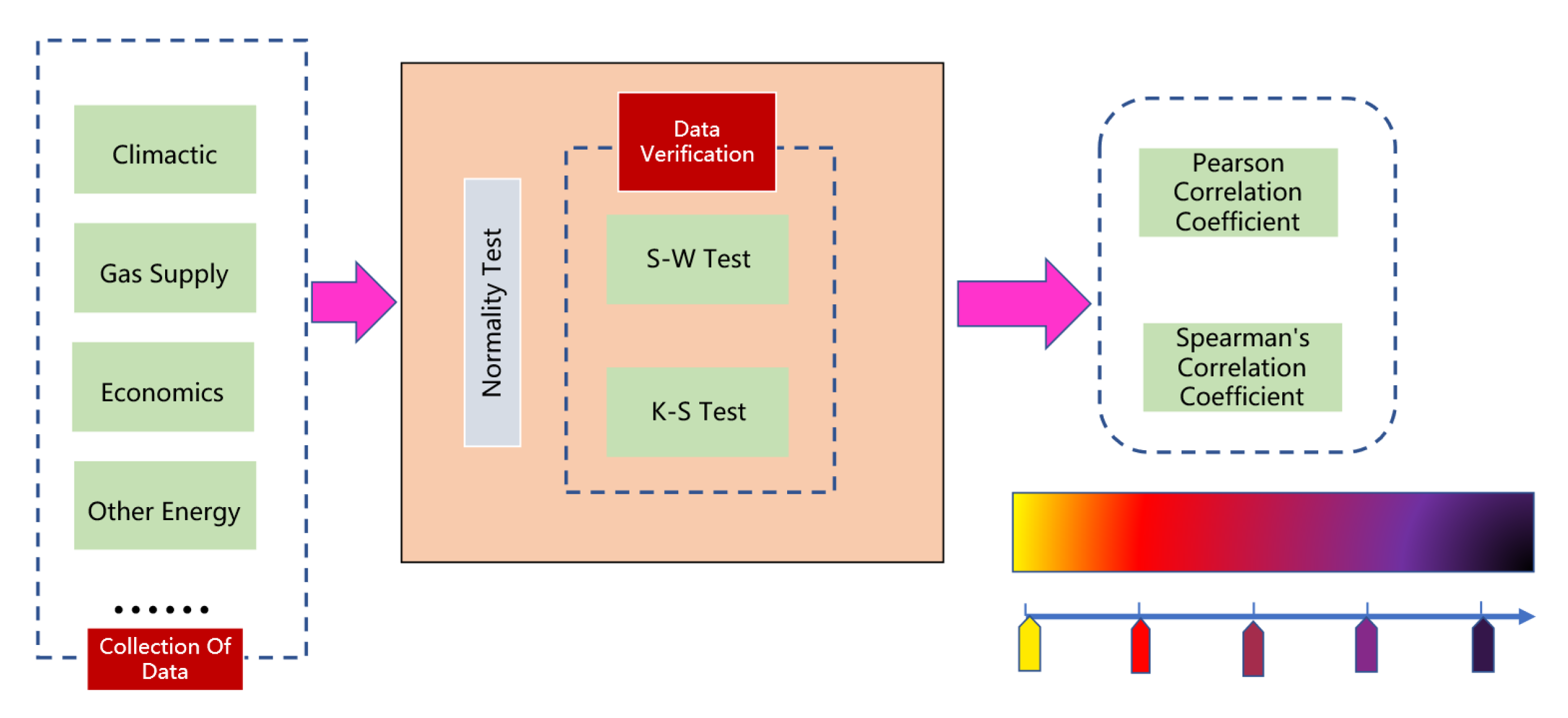
Figure 1. Relevance analysis flowchart.
Energies 18 03274 g001
The calculated correlation coefficient values based on actual data range between −1 and 1, representing the degree of correlation as shown in Table 1. However, this interpretation must be based on testing the significance of the correlation coefficient [23]. In practical applications, we typically report both the correlation coefficient and the significance (p) value. The correlation coefficient tells us the strength and direction of the linear relationship between two variables, while the p-value helps us determine whether this relationship is statistically significant.

2.1. Normality Test

The normality test is a common statistical method used to determine whether a dataset follows a normal distribution. In this study, the Shapiro–Wilk (S-W) test [24] was chosen, which is a widely recommended non-parametric test method. It is suitable for small sample sizes (N < 5000) and has a high level of accuracy [25,26]. The W value in the S-W test statistic [26] is defined as follows:
W = i = 1 n / 2 a i x n + 1 i x i 2 i = 1 n x i x ¯ 2
where n represents the sample size; xi is the ith order statistic; x ¯ is the sample mean; and ai are the weights, which can be derived from the quantile tables.
The W statistic can be viewed as the ratio of the variance-optimal estimator derived from a certain linear combination of order statistics to the sample variance of the data. Based on a given significance level α (commonly set at 0.05) and the sample size n, the critical value Wα can be determined by consulting the quantile table for the W statistic. If W < , it is concluded that the dataset does not follow a normal distribution; conversely, if W, it is considered to follow a normal distribution. Since critical values may differ depending on the method employed, statisticians often express the results in terms of probability values (p) for a more generalized decision-making outcome. Specifically, if p = P(W ≥ Wα) > α, then the dataset is deemed to follow a normal distribution [24].

2.2. Pearson Correlation Coefficient

Pearson correlation analysis is a statistical method used to assess the strength and direction of the linear relationship between two continuous variables. This correlation is represented by a value known as the Pearson correlation coefficient [27], which ranges from −1 to 1 [28]. When the absolute value of r is closer to 1, it indicates a stronger linear association between the two variables. If r is positive, it indicates a positive correlation, while a negative r indicates a negative correlation. When r approaches 0, it implies that there is no linear relationship.
r = i = 1 n x i x ¯ y i y ¯ i = 1 n x i x ¯ 2 i = 1 n y i y ¯ 2
where r is the value of the correlation coefficient; xi is the different values corresponding to the variable x; x ¯ is the average of the variable x; yi is the different values corresponding to the variable y; y ¯ is the average of the variable y; and n is the number of variables.
In practical applications, the Pearson correlation coefficient is frequently used in fields such as social sciences, biology, and medicine to study the correlations between different indicators, thereby providing a basis for further research and decision-making. However, the Pearson correlation coefficient only measures the linear correlation between two variables and may not accurately reflect non-linear relationships. Therefore, it is necessary to introduce other correlation coefficient methods as supplements, as discussed in the following chapters. It is also important to note that correlation does not imply causation. Even if there is a strong correlation between two variables, one cannot directly conclude that one variable causes change in the other. A comprehensive analysis that considers the actual situation is needed.

2.3. Spearman’s Correlation Coefficient

In statistics, the Spearman coefficient is commonly used to describe the non-linear correlation between two variables. The Spearman rank correlation coefficient, also known as just the rank correlation coefficient, is a statistic used to measure the non-linear relationship between two variables [21]. Unlike the Pearson correlation coefficient, it does not rely on a normal distribution of the dataset or linear relationships. This coefficient is calculated by ranking the values of the variables and then using these ranks to compute the covariance and standardize the result. The values range from −1 (perfect negative correlation) to 1 (perfect positive correlation), with 0 indicating no correlation. The Spearman rank correlation coefficient is suitable for handling small samples and non-normally distributed data, making it widely applicable in various research fields [29].
ρ = 1 n i = 1 n R x i R ¯ x R y i R ¯ y 1 n i = 1 n R x i R ¯ x 2 1 n i = 1 n R y i R ¯ y 2
where R(x) is the rank of x, R(y) is the rank of y, R ¯ (x) is the average rank of x, and R(y) is the average rank of y.

3. Case Studies

This case study focuses on the natural gas pipeline branches in a specific region, analysing the impact of various factors—such as climate, gas supply volume, population, and economic conditions—on scheduling decisions. The natural gas dispatch data in this section were obtained from a regional gas dispatch operator in China, consistent with the studied areas. Normality tests and correlation analyses in the case study were computed using the SPSSPRO platform https://www.spsspro.com/ (accessed on 9 April 2024).

3.1. A Correlation Study of RA Temperature

Energy datasets are characterized by nonlinearity, seasonality, and growth trends [30], making seasonal natural gas dispatch and forecasting particularly critical [31]. The impact of seasonal factors is primarily reflected in climatic conditions. Therefore, this case study selected average temperature and historical extreme temperatures as representative climatic influencing factors.
Temperature data for Region RA from November to May was collected from Weather.com [32], with both dispatch and temperature data corresponding to the same region and time period. All datasets are presented in Table 2.

3.1.1. RA Temperature Normality Test

The analysis results are presented in Table 3. The proximity between the mean and median values of all variables suggests the absence of significant outliers. Notably, the historical minimum temperature exhibited the highest standard deviation (5.56 °C) and skewness (1.061), indicating potential right-tailed outliers.
The Shapiro–Wilk test revealed no significant deviation from a normal distribution for any variables (p > 0.05). However, the low kurtosis (−1.509) of gas output suggests a more dispersed distribution than found in a typical normal distribution, likely reflecting the dynamic influence of multiple factors on gas consumption patterns.

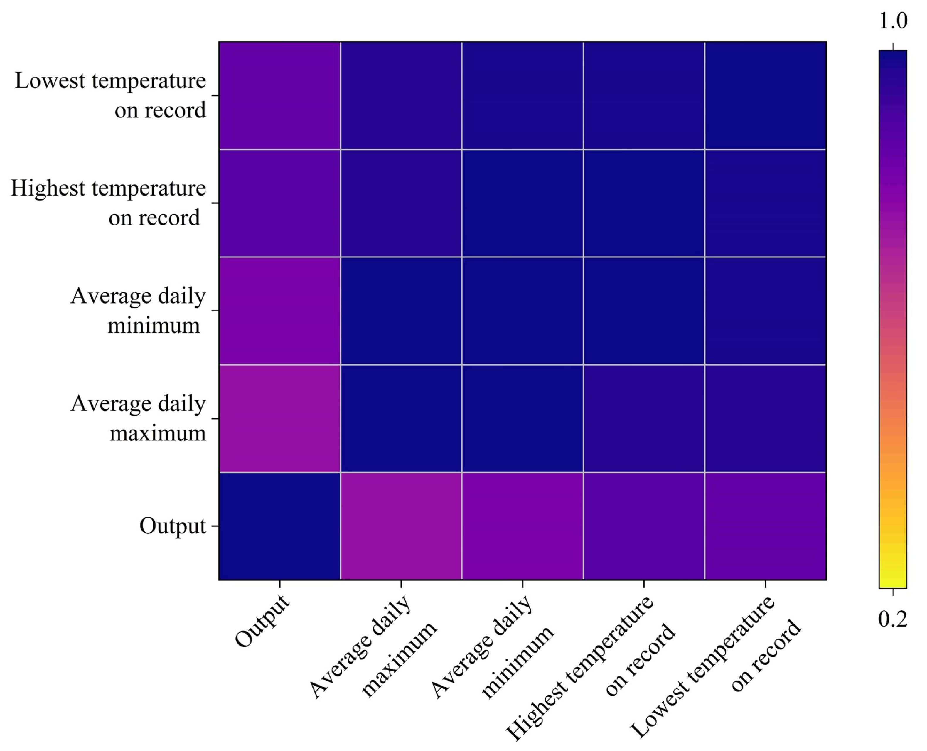
3.1.2. RA Temperature Pearson Correlation Analysis

Based on these normality test results showing no significant deviations (p > 0.05), Pearson correlation analysis was conducted to evaluate pairwise relationships between variables (Table 4). The analysis revealed two key findings: First, temperature indicators demonstrate severe multicollinearity with strong inter-correlations, suggesting they should not all be included simultaneously in the dispatch system. Second, consistent positive correlations exist between the temperature metrics and the branch-line average gas output.
The correlations between the variables can be illustrated by the heatmap shown in Figure 2, which depicts climate relationships. It can be concluded that the average output of the RA branch is most strongly correlated with the historical maximum temperature. Statistical testing indicates that there is only a 1% chance that the observed differences are due to random factors, meaning that 99% are attributed to non-random factors. In contrast, the average output shows a weaker correlation with other temperature types; however, it can still be inferred that there is only a 5% chance that the observed differences are due to random factors, suggesting that 95% of the differences arise from non-random influences.

3.2. A Correlation Study of Gas Supply to Pipeline Networks

A natural gas pipeline network is a critical infrastructure connecting the upstream supply side and the downstream demand side, making a stable and resilient gas supply through the pipeline network an important research area [33]. Therefore, this case study investigated the relationship between the upstream gas supply and downstream pipeline gas dispatch operations, specifically taking the pipeline network in Region A as an example to analyse the correlations between the total gas supply in this region and the following pipelines: the AI-LNG West Line, HA-BR Line, KI Line, TH-HA Line, ZK-KN Line, SZ Branch, EH Branch, and WE Branch. All these pipelines belong to the same Region A and are spatially consistent.

3.2.1. Gas Supply Normality Test

The analysis results are shown in Table 5. The gas inflow volumes of most pipelines significantly deviate from a normal distribution (Shapiro-Wilk test p < 0.01). Among them, the WE Branch demonstrates extreme right-skewness (skewness = 2.202) and leptokurtic characteristics (kurtosis = 4.435), indicating the presence of high outlying values.
The KI Line is the only pipeline that approximates a normal distribution (p = 0.091). Left-skewed variables (such as total gas inflow and the SZ Branch) suggest there were occasional days with relatively low inflow volumes.

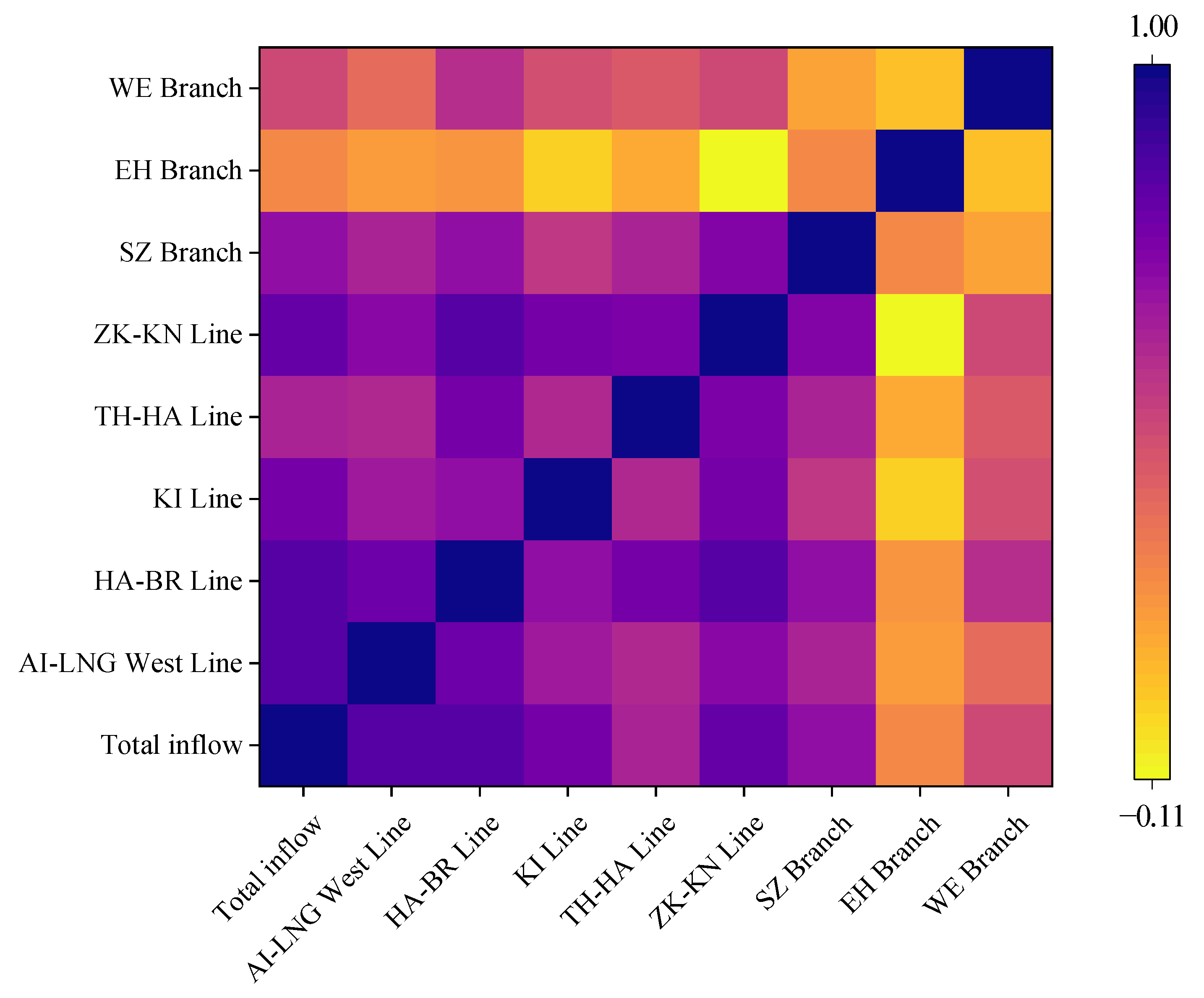
3.2.2. Gas Supply Spearman Correlation Analysis

The normality tests showed that both the total gas inflow and most pipelines’ inflow volumes significantly deviated from a normal distribution. Therefore, Spearman’s correlation analysis was used in this case, with analytical steps similar to Pearson’s correlation. Specific results are shown in Table 6.
The results indicate that all pipelines showed significant positive correlations with total gas inflow. The EH and WE branch lines exhibited stronger independence with weaker correlations for other pipelines.
The above table presents the parameter results of the model verification, including correlation coefficients and significance p-values. The correlations between the variables can be visually represented by the heatmap in Figure 3. It can be concluded that the total inflow is best correlated with the AI-LNG West Line, HA-BR Line, KI Line, TH-HA Line, SZ Branch, ZK-KN Line, and WE Branch, indicating that there is only a 1% chance that the observed differences are due to random factors. In comparison, 99% of the differences arise from non-random factors. In contrast, the correlation between total inflow and the EH Branch has only a 5% chance of being attributed to random factors, suggesting that 95% of the differences are due to non-random influences.

3.3. Population-Economy Correlation Studies

Economic development level, population size, and structure positively influence natural gas consumption [34]. However, different demographic and economic indicators exhibit varying correlations with natural gas dispatch. To verify and select the indicators most representative of natural gas pipeline network dispatch, this case study examined the correlations between gas outflow volumes of eight branch lines (YX, LJ, DJ, GL, RA, HC, FCG, and YL) and three regional indicators: permanent resident population, GDP, and per capita GDP. The data for permanent resident population, GDP, and per capita GDP were obtained from the China Statistical Information Network [35].
The service areas of these eight natural gas branch lines strictly correspond to prefecture-level city administrative boundaries and are all located within the same region. The permanent resident population, GDP, and per capita GDP data use 2022 statistical data from the respective prefecture-level administrative divisions where each branch line is located, ensuring spatial scale consistency. Specific data are shown in Table 7.

3.3.1. Population-Economy Normality Test

The test results presented in Table 8 demonstrate that the gas outflow dataset displays significant right-skewness (skewness = 2.131) and leptokurtic characteristics (kurtosis = 5.045), with the Shapiro–Wilk test confirming a non-normal distribution (W = 0.753, p = 0.009). In comparison, both GDP (W = 0.918, p = 0.411) and permanent resident population (W = 0.940, p = 0.611) satisfy the normality assumption, while per capita GDP shows borderline non-significant deviations from normality (p = 0.065) but still exhibits a right-skewed tendency (skewness = 1.288).

3.3.2. Population-Economy Spearman Correlation Analysis

Since the gas outflow dataset showed a non-normal distribution, Spearman’s correlation test was selected for this case study. The specific results are shown in Table 9. Per capita GDP showed a marginally significant positive correlation with natural gas outflow (r = 0.667, p = 0.071), while the effects of total GDP and population size did not reach statistical significance.
The correlations between the variables can be intuitively illustrated by the heatmap shown in Figure 4. The Spearman test p-value for the relationship between gas output and GDP, resident population, and per capita GDP is 0.183, 0.82, and 0.071, respectively. The p-value was used to assess the significance of the observed rank correlations between the variables while conducting the Spearman rank correlation test. A smaller p-value typically indicates a more significant correlation, while a larger p-value suggests a weaker correlation. The relationship between gas output and GDP and the resident population is insignificant, while there is a certain correlation with per capita GDP. These results indicate a relatively strong correlation between natural gas dispatch demand and per capita GDP. This is primarily because per capita GDP can more accurately reflect residents’ living standards and consumption capabilities, directly influencing the demand for clean energy such as natural gas. In contrast, while population size and total GDP are important economic indicators, their correlation with natural gas dispatch demand is relatively weaker in this context.

3.4. Correlation Studies of Energy Coupling

Integrated Energy Systems (IESs), as an innovative solution to global energy challenges, have achieved improvements in energy efficiency and reductions in carbon emissions through multi-energy coordination and intelligent optimization technologies [36,37]. By coupling various energy networks such as electricity, heating, and gas, an IES establishes an integrated “source–grid–load–storage” framework. The introduction of power-to-gas (P2G) and gas-to-power (G2P) technologies has enhanced the flexibility of natural gas and power systems [38]. Coal and its derivatives are used to produce methane, enabling cleaner utilization of coal resources [39]. Therefore, studying the usage of other energy sources is essential for research on natural gas pipeline network dispatch.
Jiangsu Province, as a major economic powerhouse in China, serves as a benchmark for future development, with its energy coupling system predominantly found in the industrial sector. Therefore, this study investigated the correlation between natural gas and other energy sources based on the primary energy consumption of large-scale industrial enterprises in Jiangsu Province from 2011 to 2021. In this case study, natural gas was selected as the research target alongside electricity, coal, crude oil, and liquefied petroleum gas (LPG), with specific data illustrated in the Table 10.

3.4.1. Energy Coupling Normality Test

The test results in Table 11 show that electricity (W = 0.959, p = 0.779) and raw coal (W = 0.940, p = 0.557) consumption meet the normality assumption. Crude oil consumption exhibits significant left-skewness (skewness = −1.333) and non-normal characteristics (W = 0.831, p = 0.034), suggesting the use of Spearman’s correlation analysis. Notably, although natural gas consumption does not reject the normality hypothesis (p = 0.175), its severely low kurtosis (−1.879) indicates an abnormally flat data distribution.

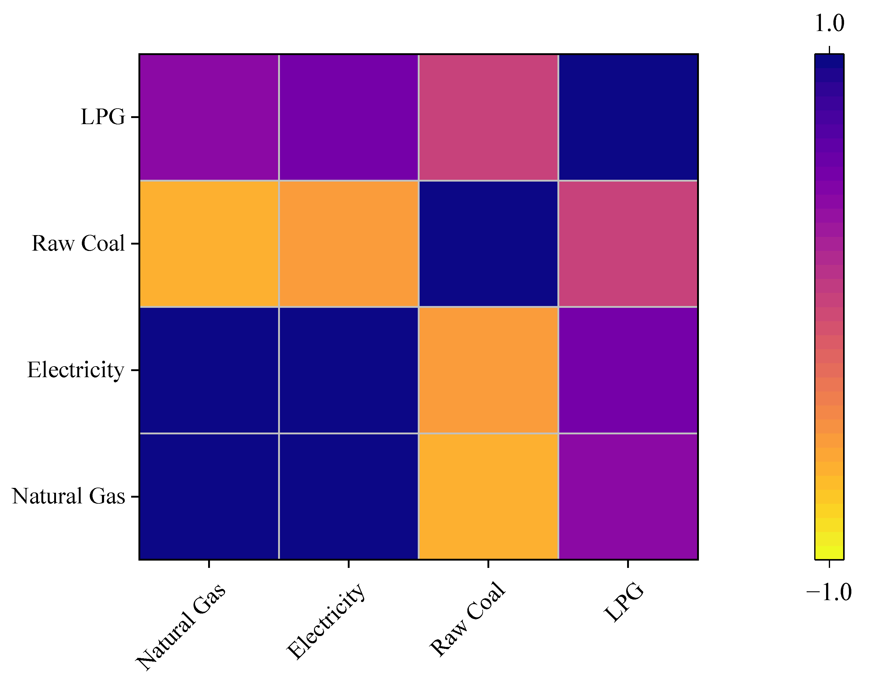
3.4.2. Energy Coupling Pearson Correlation Analysis

Natural gas, electricity, and raw coal consumption exhibit normal distributions, so Pearson correlation analysis was selected. The results are shown in Table 12, where the correlation patterns are clearly visible: natural gas consumption shows a significant positive correlation with electricity consumption, a significant negative correlation with raw coal consumption, and minimal correlation with liquefied petroleum gas consumption.
The correlations between variables can be visually observed in Figure 5. The Pearson correlation coefficient between natural gas consumption and electricity, raw coal, and liquefied petroleum gas (LPG) consumption is 0.973, −0.641, and 0.427, respectively. Natural gas consumption shows a significant positive correlation with electricity consumption, a significant negative correlation with raw coal consumption, and essentially no correlation with LPG consumption. These results demonstrate the coordinated operation between natural gas and power systems, as well as the environmental policy of replacing coal with gas. Although both natural gas and LPG are fossil fuels, they serve as substitutes in many applications, such as household cooking and heating. Due to differences in their markets and applications, their consumption levels may not show a significant correlation. LPG is more commonly used in areas without access to natural gas pipelines or as an alternative fuel to gasoline and diesel.

3.4.3. Spearman Correlation Analysis

Due to the crude oil dataset not conforming to a normal distribution, the Spearman correlation coefficient method was chosen for the correlation analysis between crude oil and natural gas data. The specific results of the test are shown in Table 13.
Figure 6 clearly shows through the heatmap that natural gas consumption exhibits a strong positive correlation with crude oil consumption, with a Spearman test p-value of 0.806.

4. Conclusions

This study focused on factors such as climate temperature, total gas supply, population size, GDP, and per capita GDP. The Pearson correlation coefficient with the historical maximum temperature is 0.878, and with the historical minimum temperature, it is 0.809. The correlations with average daily maximum and minimum temperatures follow, with Pearson correlation coefficients of 0.756 and 0.809, respectively, indicating good correlations.
Through the Spearman correlation test, it was found that the total gas inflow had a significant statistical correlation with the AI-LNG West Line, HA-BR Line, KI Line, TH-HA Line, ZK-KN Line, SZ Branch, and WE Branch, all showing positive correlations. This indicates a strong relationship between total gas inflow and these variables, with correlation coefficients of 0.82, 0.83, 0.746, 0.576, 0.78, 0.663, and 0.434, respectively. The correlation with the EH Branch was slightly weaker but still significant at the 5% level, with a Spearman correlation coefficient of 0.201. Further Spearman correlation analysis revealed that the output of the YX, LJ, DJ, GL, RA, HC, FCG, and YL branches showed no significant correlation with the regional resident population or GDP but had a correlation with per capita GDP at the 10% significance level, with a correlation coefficient of 0.667. The analysis of multiple factors confirmed that natural gas scheduling is significantly related to several external factors.
Natural gas consumption also showed strong correlations with the primary energy sources. Among them, the correlation with electricity consumption was the strongest, with a Pearson correlation coefficient of 0.973, while the Pearson correlation coefficient with coal consumption was −0.641. The Spearman correlation test revealed the correlation coefficient between natural gas and crude oil consumption was 0.806. These results highlight the system-wide or complementary roles of different energy sources. Furthermore, the case study on energy consumption in Jiangsu Province also revealed positive and negative correlations, indicating a strong positive correlation between natural gas consumption and electricity and crude oil consumption and a strong negative correlation with coal consumption.
In conclusion, natural gas scheduling demand strongly correlates with climate, gas supply, and per capita GDP. Natural gas consumption also strongly correlates with electricity, crude oil, and coal consumption. However, different factors may lead to varying correlations with natural gas scheduling demand due to differences in energy usage habits and the development of natural gas pipeline infrastructure across regions. Therefore, conducting specific analyses tailored to different pipeline network systems and regional characteristics will help more accurately identify key external factors, thereby enhancing the scientific rigor and foresight of natural gas dispatch. Pipeline operators and relevant administrative departments can formulate response strategies based on the following points:
(1)
Dynamic Dispatch Optimization: Operators can establish demand response models based on climate forecasts and macroeconomic indicators to dynamically adjust gas supply plans.
(2)
Multi-Energy Coordinated Management: In regions with peak electricity or coal consumption, special attention should be paid to the coupling relationship between natural gas and alternative energy sources to avoid short-term supply–demand imbalances caused by energy substitution effects.
(3)
Differentiated Infrastructure Planning: For areas with insufficient pipeline coverage but rapid demand growth, infrastructure improvements should be prioritized, while dispatch strategies should be aligned with local energy consumption patterns.
This study did not fully consider the operational characteristics of driving devices (such as electric compressors or gas turbine-driven compressors) in natural gas pipeline networks. There exists complex dynamic coupling relationships between the operating status of these critical equipment, environmental parameters, and pipeline flow rates. Future research will focus on establishing correlation models between multi-time-scale operational signals of driving devices and pipeline network dispatch decisions to enhance the completeness of system analysis.

Author Contributions

Conceptualization, C.W. and B.W. (Bohong Wang); Methodology, C.W. and B.W. (Bohong Wang); Software, W.Z.; Validation, C.W., N.X., and B.W. (Bosen Wang); Formal Analysis, N.J.; Investigation, W.Z.; Resources, N.X.; Data Curation, C.W.; Writing—Original Draft Preparation, C.W.; Writing—Review & Editing, B.W. (Bohong Wang) and B.W. (Bosen Wang); Visualization, W.Z.; Supervision, B.W. (Bohong Wang); Project Administration, N.J.; Funding Acquisition, B.W. (Bohong Wang). All authors have read and agreed to the published version of the manuscript.

Funding

This research was funded by the National Natural Science Foundation of China, grant number 52302420.

Data Availability Statement

Data can be made available on request from the corresponding author.

Conflicts of Interest

Author Ning Jia was employed by the company Northwest Sichuan Division, PetroChina Southwest Oil & Gas Field Company. The remaining authors declare that the research was conducted in the absence of any commercial or financial relationships that could be construed as a potential conflict of interest.

Nomenclature

S-WShapiro–Wilk
GDPGross Domestic Product
LPGLiquefied Petroleum Gas

References

  1. Hong, B.; Wang, C.; Zhang, K.; Lim, J.S.; Varbanov, P.S.; Jia, X.; Ji, M.; Tao, H.; Li, Z.; Wang, B. Carbon Emission Pinch Analysis for Shipping Fuel Planning Considering Multiple Period and Fuel Conversion Rates. J. Clean. Prod. 2023, 415, 137759. [Google Scholar] [CrossRef]
  2. Liu, H.; Liu, Y.; Wang, C.; Song, Y.; Jiang, W.; Li, C.; Zhang, S.; Hong, B. Natural Gas Demand Forecasting Model Based on LASSO and Polynomial Models and Its Application: A Case Study of China. Energies 2023, 16, 4268. [Google Scholar] [CrossRef]
  3. Zhao, W.; Wang, B.; Pan, T.; Chen, Y.; Tao, H.; Guo, B.; Varbanov, P.S.; Lu, J. Optimization of Island Integrated Energy System based on Marine Renewable Energy. Fundam. Res. 2024, in press. [Google Scholar] [CrossRef]
  4. Energy Institute. Statistical Review of World Energy 2024. Available online: https://www.energyinst.org/statistical-review/home (accessed on 26 September 2024).
  5. Huang, Y.; Qin, G.; Yang, M.; Nogal, M. Dynamic Quantitative Assessment of Service Resilience for Long-Distance Energy Pipelines under Corrosion. Reliab. Eng. Syst. Saf. 2025, 256, 110792. [Google Scholar] [CrossRef]
  6. Wei, X.; Qiu, R.; Zhang, B.; Liu, C.; Wang, G.; Wang, B.; Liang, Y. Operation Optimization of Large-Scale Natural Gas Pipeline Networks Based on Intelligent Algorithm. Energy 2024, 310, 133258. [Google Scholar] [CrossRef]
  7. Wang, B.; Hao, H. Process Integration in Optimising the Oil and Gas Supply Chain. J. Sustain. Dev. Indic. 2025, 1, 1–20. [Google Scholar] [CrossRef]
  8. Peng, J.; Zhou, J.; Liang, G.; Li, C.; Qin, C. Multi-Period Integrated Scheduling Optimization of Complex Natural Gas Pipeline Network System with Underground Gas Storage to Ensure Economic and Environmental Benefits. Energy 2024, 302, 131837. [Google Scholar] [CrossRef]
  9. Özmen, A. Sparse Regression Modeling for Short- and Long-term Natural Gas Demand Prediction. Ann. Oper. Res. 2023, 322, 921–946. [Google Scholar] [CrossRef]
  10. Bazyar, A.; Zarrinpoor, N.; Safavian, A. Optimal Design of a Sustainable Natural Gas Supply Chain Network under Uncertainty. Chem. Eng. Res. Des. 2021, 176, 60–88. [Google Scholar] [CrossRef]
  11. Sesini, M.; Giarola, S.; Hawkes, A.D. Strategic Natural Gas Storage Coordination among EU Member States in Response to Disruption in the Trans Austria Gas Pipeline: A Stochastic Approach to Solidarity. Energy 2021, 235, 121426. [Google Scholar] [CrossRef]
  12. Oke, D.; Mukherjee, R.; Sengupta, D.; Majozi, T.; El-Halwagi, M. On the Optimization of Water-Energy Nexus in Shale Gas Network under Price Uncertainties. Energy 2020, 203, 117770. [Google Scholar] [CrossRef]
  13. Liu, Z.E.; Long, W.; Chen, Z.; Littlefield, J.; Jing, L.; Ren, B.; El-Houjeiri, H.M.; Qahtani, A.S.; Jabbar, M.Y.; Masnadi, M.S. A Novel Optimization Framework for Natural Gas Transportation Pipeline Networks Based on Deep Reinforcement Learning. Energy AI 2024, 18, 100434. [Google Scholar] [CrossRef]
  14. Peng, Y.; Qiu, R.; Zhao, W.; Zhang, F.; Liao, Q.; Liang, Y.; Fu, G.; Yang, Y. Efficient Energy Optimization of Large-Scale Natural Gas Pipeline Network: An Advanced Decomposition Optimization Strategy. Chem. Eng. Sci. 2025, 309, 121456. [Google Scholar] [CrossRef]
  15. Fan, L.; Su, H.; Wang, W.; Zio, E.; Zhang, L.; Yang, Z.; Peng, S.; Yu, W.; Zuo, L.; Zhang, J. A Systematic Method for the Optimization of Gas Supply Reliability in Natural Gas Pipeline Network Based on Bayesian Networks and Deep Reinforcement Learning. Reliab. Eng. Syst. Saf. 2022, 225, 108613. [Google Scholar] [CrossRef]
  16. Yan, Y.; Yan, J.; Liu, S.; Wang, Y.; Wang, B.; Han, S.; Yongqian, L. Review and Prospect on the Construction Method of Security Region for Integrated Natural Gas and Power Systems. Energy 2024, 307, 132543. [Google Scholar] [CrossRef]
  17. Huang, H.; Zhang, A.; Xu, X.; Li, Q.; Yang, W.; Qu, G. Optimal Scheduling of Bidirectional Coupled Electricity-Natural Gas Systems Based on Multi-Port Gas Network Equivalent Model. Int. J. Electr. Power Energy Syst. 2022, 139, 108049. [Google Scholar] [CrossRef]
  18. Yan, Y.; Wang, Y.; Yan, J.; Zhang, H.; Shang, W. Wind Electricity-hydrogen-Natural Gas Coupling: An Integrated Optimization Approach for Enhancing Wind Energy Accommodation and Carbon Reduction. Appl. Energy 2024, 369, 123482. [Google Scholar] [CrossRef]
  19. Messini, E.M.B.; Bourek, Y.; Ammari, C.; Pesyridis, A. The Integration of Solar-Hydrogen Hybrid Renewable Energy Systems in Oil and Gas Industries for Energy Efficiency: Optimal Sizing Using Fick’s Law Optimisation Algorithm. Energy Convers. Manag. 2024, 308, 118372. [Google Scholar] [CrossRef]
  20. Pearson, K. III. Contributions to the Mathematical Theory of Evolution. Proc. R. Soc. Lond. 1894, 54, 329–333. [Google Scholar] [CrossRef]
  21. Myers, J.L.; Well, A.D.; Lorch, R.F., Jr. Research Design and Statistical Analysis, 3rd ed.; Routledge: New York, NY, USA, 2010; ISBN 978-0-203-72663-1. [Google Scholar]
  22. Xu, L.; Wen, S.; Huang, H.; Tang, Y.; Wang, Y.; Pan, C. Corrosion Failure Prediction in Natural Gas Pipelines Using an Interpretable XGBoost Model: Insights and Applications. Energy 2025, 325, 136157. [Google Scholar] [CrossRef]
  23. Jia, J.; He, X.; Jin, Y. Statistics, 8th ed.; A series of textbooks on statistics for the 21st century; Renmin University Press: Beijing, China, 2021; ISBN 978-7-300-29310-3. [Google Scholar]
  24. Shapiro, S.S.; Wilk, M.B. An Analysis of Variance Test for Normality (Complete Samples). Biometrika 1965, 52, 591–611. [Google Scholar] [CrossRef]
  25. de Souza, R.R.; Toebe, M.; Mello, A.C.; Bittencourt, K.C. Sample Size and Shapiro-Wilk Test: An Analysis for Soybean Grain Yield. Eur. J. Agron. 2023, 142, 126666. [Google Scholar] [CrossRef]
  26. Razali, N.M.; Wah, Y.B. Power Comparisons of Shapiro-Wilk, Kolmogorov-Smirnov, Lilliefors and Anderson-Darling Tests. J. Stat. Model. Anal. 2011, 2, 21–33. [Google Scholar]
  27. Zhou, H.; Deng, Z.; Xia, Y.; Fu, M. A New Sampling Method in Particle Filter Based on Pearson Correlation Coefficient. Neurocomputing 2016, 216, 208–215. [Google Scholar] [CrossRef]
  28. Gong, H.; Li, Y.; Zhang, J.; Zhang, B.; Wang, X. A New Filter Feature Selection Algorithm for Classification Task by Ensembling Pearson Correlation Coefficient and Mutual Information. Eng. Appl. Artif. Intell. 2024, 131, 107865. [Google Scholar] [CrossRef]
  29. Jiang, J.; Zhang, X.; Yuan, Z. Feature Selection for Classification with Spearman’s Rank Correlation Coefficient-Based Self-Information in Divergence-Based Fuzzy Rough Sets. Expert Syst. Appl. 2024, 249, 123633. [Google Scholar] [CrossRef]
  30. Yan, S.; Peng, M.; Wu, L.; Xiong, P. A Novel Structural Adaptive Seasonal Grey Bernoulli Model in Natural Gas Production Forecasting. Eng. Appl. Artif. Intell. 2025, 148, 110407. [Google Scholar] [CrossRef]
  31. Zhang, J.; Shen, C.; Qin, Y.; Chen, J. Forecasting of Natural Gas Based on a Novel Discrete Grey Seasonal Prediction Model with a Time Power Term. Energy Strategy Rev. 2025, 58, 101677. [Google Scholar] [CrossRef]
  32. December Weather in Qinzhou, Guangxi _Qinzhou December Weather_Qinzhou December Weather Temperature_Qinzhou December Average Weather Temperature, Temperature_Weather.com. Available online: https://www.tianqi.com/qiwen/city-qinzhou-12/ (accessed on 7 April 2024).
  33. Zhao, Z.; Yang, Z.; Su, H.; Faber, M.H.; Zhang, J. A Methodology of Natural Gas Pipeline Network System Supply Resilience Optimization: Based on Demand-Side and Data Science-Driven Approach. Reliab. Eng. Syst. Saf. 2025, 261, 111071. [Google Scholar] [CrossRef]
  34. Xu, G.; Chen, Y.; Yang, M.; Li, S.; Marma, K.J.S. An Outlook Analysis on China’s Natural Gas Consumption Forecast by 2035: Applying a Seasonal Forecasting Method. Energy 2023, 284, 128602. [Google Scholar] [CrossRef]
  35. China Statistical Information Network—China Statistical Yearbook 2023. Available online: http://www.tjcn.org/ (accessed on 11 April 2024).
  36. Kou, Y.; Bie, Z.; Li, G.; Liu, F.; Jiang, J. Reliability Evaluation of Multi-Agent Integrated Energy Systems with Fully Distributed Communication. Energy 2021, 224, 120123. [Google Scholar] [CrossRef]
  37. Li, H.; Liu, H.; Ma, J.; Wang, J. Robust Stochastic Optimal Dispatching of Integrated Electricity-Gas-Heat System Considering Generation-Network-Load Uncertainties. Int. J. Electr. Power Energy Syst. 2024, 157, 109868. [Google Scholar] [CrossRef]
  38. Shabanian-Poodeh, M.; Hooshmand, R.-A.; Shafie-khah, M. Reliability-Constrained Configuration Optimization for Integrated Power and Natural Gas Energy Systems: A Stochastic Approach. Reliab. Eng. Syst. Saf. 2025, 254, 110600. [Google Scholar] [CrossRef]
  39. Chyou, Y.-P.; Chiu, H.-M.; Chen, P.-C.; Chien, H.-Y.; Wang, T. Coal-Derived Synthetic Natural Gas as an Alternative Energy Carrier for Application to Produce Power—Comparison of Integrated vs. Non-Integrated Processes. Energy 2023, 282, 128958. [Google Scholar] [CrossRef]
  40. Liu, H.; Liu, Y.; Yang, J.; Men, Z.; Wang, C. Forecast of Natural Gas Consumption in Jiangsu Province Based on Combination Forecast. Proc. SPIE 2023, 12642, 1264208. [Google Scholar] [CrossRef]
  41. Statistical Bureau of Jiangsu Province. Available online: https://tj.jiangsu.gov.cn/ (accessed on 11 May 2024).
Figure 2. Heatmaps of climate relationships.
Energies 18 03274 g002
Figure 3. Heatmap of gas supply and discharge.
Energies 18 03274 g003
Figure 4. Heatmaps of demographic and economic conditions.
Energies 18 03274 g004
Figure 5. Energy coupled Pearson heatmap.
Energies 18 03274 g005
Figure 6. Natural gas vs. crude oil heatmap.
Energies 18 03274 g006
Table 1. Table of correlation coefficients.
The Absolute Value of Correlation CoefficientInterpretation
0.8–1.0Highly correlated
0.5–0.8Moderately correlated
0.3–0.5Lowly correlated
0–0.3Very weakly correlated or uncorrelated
Table 2. RA temperature and average daily gas output.
MonthsAverage Daily Maximum Temperature/°CAverage Daily Minimum Temperature/°CHighest Temperature on Record/°CLowest Temperature on Record/°CAverage Gas Output from Branch Lines/105 m3
Nov.2619319121.73
Dec.2013284116.64
Jan.1812283121.85
Feb.1913295131.62
Mar.2317319134.80
Apr.28223312147.39
May.32263519149.83
Table 3. RA temperature test results.
Variable NameSample SizeMedianAverage ValueStandard DeviationSkewnessKurtosisS-W Test
Average daily maximum temperature/°C72323.7145.1870.529−0.9980.937 (0.610)
Average daily minimum temperature/°C71717.4295.2550.636−0.8250.913 (0.414)
Highest temperature
on record/°C
73130.7142.6280.587−0.6830.916 (0.436)
Lowest temperature
on record/°C
798.7145.5591.0610.9810.906 (0.366)
Average gas output
from branch lines/105 m3
7131.621131.9812.9560.391−1.5090.911 (0.400)
Note: Values in parentheses are p-values.
Table 4. Correlation coefficient table.
Variable NameAverage Gas Output from Branch Lines/105 m3Average Daily Maximum Temperature/°CAverage Daily Minimum Temperature/°CHighest Temperature on Record/°CLowest Temperature on Record/°C
Average gas output from branch lines/105 m31
(0.000 ***)
Average daily maximum temperature/°C0.756
(0.049 **)
1
(0.000 ***)
Average daily minimum temperature/°C0.809
(0.027 **)
0.996
(0.000 ***)
1
(0.000 ***)
Highest temperature on record/°C0.878
(0.009 ***)
0.971
(0.000 ***)
0.988
(0.000 ***)
1
(0.000 ***)
Lowest temperature on record/°C0.841
(0.018 **)
0.968
(0.000 ***)
0.98
(0.000 ***)
0.986
(0.000 ***)
1
(0.000 ***)
Note: ***, and ** represent 1% and 5% significance levels, respectively.
Table 5. Gas supply normality test.
Variable NameSample SizeMedianAverage ValueStandard DeviationSkewnessKurtosisS-W Test
Total gas inflow/105 m31003528.463360.16669.262−0.791−0.0930.932 (0.000 ***)
AI-LNG West Line/105 m3100670.728615.277219.125−0.571−0.8570.925 (0.000 ***)
HA-BR Line/105 m3100582.085530.446254.237−0.282−0.9250.953 (0.001 ***)
KI Line/105 m3100386.693395.01171.9520.3970.1710.978 (0.091 *)
TH-HA Line/105 m31009.2918.4462.297−0.227−1.0950.939 (0.000 ***)
SZ Branch/105 m310054.03847.56316.033−0.769−0.830.869 (0.000 ***)
ZK-KN Line/105 m310080.48565.26233.368−0.151−1.7170.847 (0.000 ***)
EH Branch/105 m310078.91986.63650.2430.7530.4450.951 (0.001 ***)
WE Branch/105 m3100148.38157.05323.0392.2024.4350.704 (0.000 ***)
Note: ***, and * represent 1% and 10% significance levels, respectively.
Table 6. Spearman’s correlation analysis of gas supply and gas outflow.
Variable NameTotal Gas Inflow/105 m3AI-LNG West Line/105 m3HA-BR Line/105 m3KI Line/105 m3TH-HA Line/105 m3SZ Branch/105 m3ZK-KN Line/105 m3EH Branch/105 m3WE Branch/105 m3
Total gas inflow/105 m31
(0.000 ***)
AI-LNG West Line/105 m30.82
(0.000 ***)
1
(0.000 ***)
HA-BR Line/105 m30.83
(0.000 ***)
0.763
(0.000 ***)
1
(0.000 ***)
KI Line/105 m30.746
(0.000 ***)
0.618
(0.000 ***)
0.665
(0.000 ***)
1
(0.000 ***)
TH-HA Line/105 m30.576
(0.000 ***)
0.568
(0.000 ***)
0.75
(0.000 ***)
0.549
(0.000 ***)
1
(0.000 ***)
SZ Branch/105 m30.78
(0.000 ***)
0.68
(0.000 ***)
0.826
(0.000 ***)
0.744
(0.000 ***)
0.713
(0.000 ***)
1
(0.000 ***)
ZK-KN Line/105 m30.663
(0.000 ***)
0.575
(0.000 ***)
0.664
(0.000 ***)
0.501
(0.000 ***)
0.581
(0.000 ***)
0.702
(0.000 ***)
1
(0.000 ***)
EH Branch/105 m30.201
(0.045 **)
0.155
(0.124)
0.166
(0.099 *)
−0.002
(0.988)
0.11
(0.275)
−0.107
(0.290)
0.199
(0.047 **)
1
(0.000 ***)
WE Branch/105 m30.434
(0.000 ***)
0.321
(0.001 ***)
0.541
(0.000 ***)
0.417
(0.000 ***)
0.373
(0.000 ***)
0.425
(0.000 ***)
0.126
(0.213)
0.045
(0.656)
1
(0.000 ***)
Note: ***, **, and * represent 1%, 5%, and 10% significance levels, respectively.
Table 7. Population size and GDP in 2022.
Variable NameYX
Branch/105 m3
LJ
Branch 105 m3
DJ
Branch/105 m3
GL
Branch/105 m3
RA
Branch/105 m3
HC
Branch/105 m3
FCG
Branch/105 m3
YL
Branch/105 m3
Output/105 m310,5746642268242040109420771033
GDP/
Billions CNY
25216202412436191711369682167
Resident population/10422412550496332341106582
GDP per capita/CNY112,52749,60848,09349,14557,77433,30491,40637,222
Table 8. Demographic and economic normality test results.
Variable NameVariable NameSample SizeMedianAverage ValueStandard DeviationSkewnessKurtosis
Output/105 m382172.4882892.5853333.4132.1315.0450.753 (0.009 ***)
GDP/
Billions CNY
81526.271500.679871.121−0.183−1.7490.918 (0.411)
Resident population/1048277.905281.962190.7050.417−1.0870.94 (0.611)
GDP per capita/CNY849,376.26259,884.90927,643.9861.2880.6620.834 (0.065 *)
Note: ***, and * represent 1% and 10% significance levels, respectively.
Table 9. Spearman analysis of the demographic and economic situation.
Variable NameOutput/105 m3GDP/Billions CNYResident Population/104GDP Per Capita/CNY
Output/105 m31 (0.000 ***)
GDP/Billions CNY0.524 (0.183)1 (0.000 ***)
Resident population/104−0.095 (0.823)0.69 (0.058 *)1 (0.000 ***)
GDP per capita/CNY0.667 (0.071 *)0.238 (0.570)−0.429 (0.289)1 (0.000 ***)
Note: *** and * represent 1% and 10% significance levels, respectively.
Table 10. Use of energy sources in Jiangsu Province [40,41].
YearNatural Gas/Billion m3Electricity/GWhRaw Coal/10 ktCrude Oil/10 ktLPG/10 kt
20121124.34580.924,627.542942.1733.39
20131237.84956.6225,927.43382.9741.86
20141268.45012.5425,646.363498.7934.19
201516275114.724,601.863810.3233.85
201616985458.9525,775.424078.9947.51
201723355807.8924,364.763866.0635.4
201826976128.2724,215.34067.8735.97
20192819.6626423,297.554120.245.25
20202733.2637422,716.884017.8840.46
202131377101.224,949.034019.9945.79
Table 11. Energy coupled normal analysis.
Variable NameSample SizeMedianAverage ValueStandard DeviationSkewnessKurtosisS-W Test
Natural Gas/Billion m3102016.52067.73757.7470.049−1.8790.891 (0.175)
Electricity/GWh105633.425679.907789.1650.368−0.6790.959 (0.779)
Raw Coal/10 kt1024,614.724,612.211043.787−0.509−0.3130.94 (0.557)
Crude Oil/10 kt103941.973780.524387.18−1.3331.0980.831 (0.034 **)
LPG/10 kt1038.21539.3675.4750.341−1.7560.876 (0.117)
Note: ** represent 5% significance levels.
Table 12. Table of Pearson correlation coefficients for energy coupling.
Variable NameNatural Gas/Billion m3Electricity/GWhRaw Coal/10 ktLPG/10 kt
Natural Gas/Billion m31 (0.000 ***)
Electricity/GWh0.973 (0.000 ***)1 (0.000 ***)
Raw Coal/10 kt−0.641 (0.046 **)−0.502 (0.139)1 (0.000 ***)
LPG/10 kt0.427 (0.218)0.536 (0.111)0.04 (0.913)1 (0.000 ***)
Note: *** and ** represent 1% and 5% significance levels, respectively.
Table 13. Natural gas and crude oil Spearman correlation.
Variable NameNatural Gas/Billion m3Crude Oil/10 kt
Natural Gas/Billion m31 (0.000 ***)
Crude Oil/10 kt0.806 (0.005 ***)1 (0.000 ***)
Note: *** represent 1% significance levels.
Disclaimer/Publisher’s Note: The statements, opinions and data contained in all publications are solely those of the individual author(s) and contributor(s) and not of MDPI and/or the editor(s). MDPI and/or the editor(s) disclaim responsibility for any injury to people or property resulting from any ideas, methods, instructions or products referred to in the content.

