Article

Next-Level Energy Management in Manufacturing: Facility-Level Energy Digital Twin Framework Based on Machine Learning and Automated Data Collection

1
Industrial and Systems Engineering Department, Institute for a Secure and Sustainable Environment, The University of Tennessee, Knoxville, TN 37919, USA
2
Oak Ridge National Laboratory, Oak Ridge, TN 37830, USA
*
Author to whom correspondence should be addressed.
Energies 2025, 18(13), 3242; https://doi.org/10.3390/en18133242
Submission received: 17 March 2025 / Revised: 6 June 2025 / Accepted: 11 June 2025 / Published: 20 June 2025

Abstract

:
This research introduces an energy prediction framework at the facility level supported by automated data collection and machine learning models. It investigates whether reducing the prediction time scale allows for applying more complex machine learning techniques and if those techniques improve the prediction accuracy. The primary advantages of this framework lie in its automation of the energy prediction process and its provision of real-time energy data suitable for use in energy dashboards or digital twins. A sitewide dataset was created by combining 15 min energy and daily production data of five shops—assembly, battery, body (electric), body (gas), and paint—from a globally recognized electric vehicle manufacturer. Various machine learning models were evaluated on daily, weekly, and monthly datasets, including, in increasingly complex order: naïve, simple linear regression, net regularized generalized linear regression, principal component regression, k-nearest neighbor, random forest, and Bayesian regularized neural network. Compared to the current state-of-the-art energy consumption prediction for the industrial facility level, this research investigates more complex models and smaller time intervals for higher accuracy. The findings revealed that the more complex monthly models require a minimum of a year and a half of data to operate, while weekly models demand a year of data to achieve improved accuracy. Daily models can operate with only six months of data but exhibit poor performance due to reduced prediction accuracy of production. Key challenges identified include access to reliable, high-quality energy and production data and the initial demand for human labor.

1. Introduction

The future potential for energy savings in manufacturing lies in implementing energy efficiency projects and developing innovative energy monitoring and management approaches [1]. The digital twin (DT) and Internet of Things (IoT) paradigms enable enhanced visibility, awareness, and improvements in energy efficiency through the use of connected intelligent sensors and meters. This improved real-time energy consumption data can significantly enhance the ability of Energy Management Systems (EnMSs) to achieve sustained energy savings [2]. With a robust energy data collection process, energy efficiency opportunities can be identified at each level of the manufacturing process. Current methods for increasing energy efficiency in discrete part manufacturing are distinguished based on unit, multi-machine, factory, multi-facility, and supply chain levels [3]. The effectiveness of incorporating energy management into any of these levels depends on knowing the present state of consumption, historical consumption, and the system’s responsiveness to changes. This study was guided by the need to establish a data-gathering framework that facilitates energy management to achieve savings at each level. Energy prediction is often directed by ISO 50001:2018, the industry standard for implementing EnMSs [4]. However, manufacturers frequently rely on naïve or simple linear regression models for prediction, if they engage in any at all. While several industrial energy management regression software packages are available, none appear to integrate machine learning models with daily data inputs to make predictions. For example, the U.S. Department of Energy (DOE) Energy Performance Indicator Tool [5] does not offer predictive capabilities, only accommodating monthly data inputs and employing simple regression analysis. Although the DOE VERIFI (beta) tool [6] can implement more advanced regression analysis and generate visualizations and reports, it was not designed for predictive functions and could not accept daily or weekly inputs at the time of this study.
Original Equipment Manufacturers (OEMs) face increasing pressure to illustrate the sustainability of each stage in their manufacturing processes. If an OEM fails to accurately track and predict emissions generated during various manufacturing stages across the supply chain, it risks incurring unnecessary energy expenses, facing costs related to carbon taxes, and suffering negative impacts on its corporate image.
Smart manufacturing (SM), also called Industry 4.0 or the fourth industrial revolution, includes advanced technologies that allow real-time information transparency, improved decision-making, or interconnection between diverse processes [7]. Typical SM technologies include robotics, the Industrial Internet of Things (IIOT), cloud computing, and, importantly for this research, DT, machine learning (ML), and big data analytics.
DT is a virtual or digital counterpart to a physical system. The essential aspect of DT is that it is a uniform data model for describing manifold assets. Data and system integration, integration of cross-life-cycle data, and a service orientation are requirements for advancing to the DT level. A systematic review of machine learning applications for industrial energy efficiency by Narciso and Martins [8] showed that publications are increasing and are dominated by petrochemical production research. Only one of the forty-two papers reviewed predicts future energy consumption based on historical energy consumption, and it focuses on a specific process instead of the facility [9]. Recently, Moghadasi et al. [10] applied ML techniques to implement an energy management system according to ISO 50001:2018. Moghadasi’s method fulfills all the requirements of the ISO 50001 standard except the facility-level energy prediction: identifying significant energy users, defining energy performance indicators, developing a baseline, analyzing current energy performance, quantifying energy conservation opportunities, determining energy targets, and defining the energy action plan. Moghadasi et al. [10] focused on highly detailed process parameters such as steam temperature and pressure, but this study investigates production and historical energy consumption figures as predictors for energy use. Process parameters do not allow prediction in the same manner as production data. Moghadasi’s framework could be helpful in conjunction with this research, but it does not fulfill the energy prediction requirement.

2. Literature Review

This literature review presents the research questions and current status of integrating Smart Manufacturing (SM) concepts, including Digital Twin (DT), Internet of Things (IoT), and big data analytics, with energy management and facility-level energy predictions.
DT, IoT, and advanced enterprise systems are essential for future energy management research and provide excellent innovation potential as real-time data becomes available [11]. Medojevic et al. [12] stated that “without energy management overall at the center of Industry 4.0, there is no Industry 4.0”, pointing to the fundamental role that energy availability and energy reliability play in manufacturing processes.
The IoT has enabled many new efficiency advantages for both productivity and energy. The considerable benefits of combining Industry 4.0 with energy management have not been realized because plant managers lack awareness of the intimate connection between the two themes, and software tools need to be upgraded [12]. Shrouf and Miragliotta [13] reviewed production management practices that are enhanced by IoT technology and found six sets of benefits that can be achieved, including (1) finding and reducing energy waste sources, (2) improving energy-aware production scheduling, (3) reducing energy bills through demand response and reducing energy purchasing cost, (4) efficient maintenance management, (5) improving environmental reputation by meeting customer expectations and obtaining environmental certification, and (6) supporting decentralization in decision-making at production level to increase energy efficiency. Although the potential benefits of combining Industry 4.0 with energy management are apparent, there has been insufficient research to integrate these concepts at the industrial plant level. Also, collecting, transforming, integrating, modeling, storing, securing, analyzing, and presenting big data sets present significant challenges [14].
Several reviews exist on the interaction between energy management and advanced data analytics. Sievers and Blank [15] reviewed the state-of-the-art in data-driven residential and industrial energy management systems, including the system infrastructure’s design, wireless and wired communication protocols, real-time and historical data, forecasting algorithms, and objectives and optimization techniques. A detailed analysis of the research literature on energy management in manufacturing is presented by [16]. Six main lines of research in the field include (i) drivers and barriers, (ii) information and communication technologies, (iii) strategic paradigms, (iv) supporting tools and methods, (v) manufacturing process paradigms, and (vi) manufacturing performances in the trade-off. Since 2009, the number of publications has grown consistently until 2016, the last date in the study, and the authors expect it to continue increasing.
The DT paradigm has promoted sustainability in many sectors and applications. Pater and Stadnicka [17] reviewed twenty papers related to DT and sustainability to determine what problems are included within the two topics. They concluded that there are many areas where the potential of DT for sustainability has not been fully realized, which suggests combining DT with sustainability. The review by Pater and Stadnicka [17] showed that only one paper concerns energy monitoring and forecasting, and none are related to energy at the facility level.

2.1. Energy Management

Few energy prediction models have been identified for industrial factory-level applications. Ref. [18] provides a review of energy consumption forecasting models in the manufacturing industry. Out of 72 examined articles, only four have a system boundary of the entire factory. Most are related to the machine level. On further inspection of these four models, none predict facility energy consumption in a straightforward fashion, as proposed in this research. Ref. [19] proposes a generic statistical event simulation method for modeling the energy consumption behavior of machines. It is stated that this approach can be applied at the plant level, but how the approach could work is not demonstrated. Ref. [20] employs load bus data with a two-stage load estimator algorithm and state estimation theory to estimate the amount of electric power system expansion needed to serve an expanded load. The prediction is at the facility level, but no facility energy consumption prediction is presented. Ref. [21] describes an ML approach for 15 min forecasting of the electric load to reduce volatility in power generation introduced by renewables. This model shows how real-time energy data predictions can be made at the plant level, but it only forecasts 15 min into the future and is not easily implemented. Ref. [22] uses deep learning techniques for energy forecasting in a manufacturing area, but it focuses on building parameters such as workshop air temperature and humidity, does not include production as a predictor, and does not make a total facility prediction, including process equipment.
ML for commercial building energy management is much more widely adopted than it is for industrial facility energy management, so building energy management will be highlighted to demonstrate how industrial energy management could be improved. Chen et al. [23] reviewed the state of the art in interpretable machine learning for building energy management. They outlined the use cases for ML models and how to improve model interpretability. Detailed data acquisition platforms and typical applications exist in building energy management, including load prediction, fault detection and diagnosis, and occupancy behavior. Generalizing across industrial applications is more challenging due to the existence of varied processes and equipment, as well as the stochastic nature of manufacturing systems.
Not many data acquisition platforms have been proposed or implemented for the energy management of intelligent factories. Ref. [24] proposed a data acquisition platform for energy management in smart factories or buildings using openHAB, MQTT, and the Node Microcontroller Unit (NodeMCU). However, the focus is on improving communication security, and the proposed platform has not been implemented. To improve energy management in industrial factories, data acquisition platforms must be advanced.

2.2. Energy Digital Twin (DT)

The capability of a manufacturer to produce DT applications is a crucial goal for digital transformation, Industry 4.0, and SM [25]. The term “digital twin” was introduced by Michael Grieves in a 2002 product lifecycle management (PLM) presentation, although virtual replication of a product had already been realized in the aerospace industry [26]. A widely used definition given by Glaessgen and Stargel [27] reads: “DT is an integrated multi-physics, multi-scale, probabilistic simulation of a complex product and uses the best available physical models, sensor updates, etc., to mirror the life of its corresponding twin.” Another definition of DT in manufacturing is given by Garetti et al. [28]: “DT consists of a virtual representation of a production system that can run on different simulation disciplines characterized by the synchronization between the virtual and real system, thanks to sensed data, connected smart devices, mathematical models, and real-time data elaboration. The topical role within Industry 4.0 manufacturing systems is to exploit these features to forecast and optimize the behavior of the production system at each life cycle phase in real-time.”
In the next phase of DT research, several researchers have reviewed DT applications to determine a more specific definition of DT and present use cases. For example, ref. [29] categorically reviewed the DT in manufacturing applications to classify existing publications according to their type, level of integration, area of focus, and technology used. Before Kritzinger et al. [29], DT was viewed simply as a digital counterpart to a physical object, and the terms digital model, digital shadow, and DT were often used synonymously. Now, the terms can be distinguished by the level of data integration between the physical and digital counterparts. A digital model provides a digital representation of an existing or planned physical object without automated data exchange. A change in the state of the physical object has no direct effect on the digital object, and vice versa. The digital shadow refers to a one-way data flow between the state of a physical object and its corresponding digital representation. A change in the state of the physical object leads to a change in the digital object, but not vice versa. If, and only if, data flows are fully integrated into both directions between the physical and digital object, Kritzinger et al. [29] stated that you can accurately refer to it as a DT. The authors found that most papers used the term DT, while only 18% described a DT with bidirectional data transfer. Using the Kritzinger et al. [29] framework, we could not characterize a real-time energy information model as DT unless it had bidirectional data-transfer capability.
Shao and Helu [30] characterized DT perspectives based on the proposed definition, the relevant viewpoint (product, process, or system), the fidelity of the digital representation (complete or partial), and the temporal integration (real-time or offline). An offline DT would be where real-time communication is not critical and a periodic connection is sufficient. The authors argue that the DT concept should depend on the context and viewpoint for the specific use case and propose three critical factors for assessing the scope and requirements of a DT, including (1) Application, (2) Viewpoint, and (3) Context. A DT needs only to collect the data relevant to the use case of interest, rather than all available data. The Shao and Helu [30] framework would enable practitioners to consider an energy information model based on data in 15 min steps, as a DT application without the real-time bidirectional data-transfer capability. The currently under development ISO 23247 will provide a generic DT manufacturing development framework that considers the context and viewpoint for specific use cases. Yu et al. [31] proposed the Energy Digital Twin (EDT) concept, aiming to manage and optimize site operations to minimize specific energy consumption through four attributes, including (1) looks-like, (2) behaves-like, (3) connected-to, and (4) timescale. Yu et al. (2022) [31] classified EDT, subtly shifting from Kritzinger et al. [29] by introducing the term “Digital Manager” to describe the connected-to attribute and avoid the requirement for bi-directional transfer. The argument is that many EDT applications, such as plant evolution and retrofit, do not rely on two-way, real-time data communication but should still be counted under the broader DT class. Additionally, enabling communication from the DT back into the production environment for bi-directional data transfer requirements may require some disruption to production, which is typically avoided in manufacturing. For this research, automated data collection and integration into the digital model is the goal for energy management DT and not bidirectional data transfer, and we will refer to the application as a DT according to the DT definition from Shao and Helu [30] and the EDT definition from Yu et al. [31].
The DT concept has been fully implemented and validated in several applications, though there is a lack of a proven plant-level energy management DT. Haag and Anderl [32] prove the DT concept with a physical twin of a bending beam test bench, a DT CAD model, an MQTT broker to connect the physical and DT, a web-based dashboard, and a finite element method (FEM) simulation. The results demonstrate that the DT concept can be applied to actual systems. A challenge for DT applications is that current CAx models are designed for use in product development and are not designed to live on as DTs, which adapt to the product characteristics throughout its entire operational phase. Additionally, traditional data collection and processing methods are inadequate.
Tao et al. [33] reviewed DT’s state-of-the-art research and development history and summarized its industrial applications. The most popular application area is prognostics and health management (PHM). Energy efficiency or energy monitoring was not explicitly identified. Assad et al. [34] demonstrated the implementation of a web-based DT (WDT) for improving sustainability in industrial cyber-physical systems, proving that the energy management DT is feasible at the machine level. The three steps are (a) accessing the control parameters influencing energy consumption, (b) logging the energy consumption data, and (c) producing predictions using a computational algorithm. An industrial case study in a battery assembly production line demonstrates the WDT architecture, which has WebGL, Node.js, OPC UA server, and PLC as its major components and uses WebSocket as the communication protocol. Our paper proposes an energy management DT framework for the plant level rather than the machine level.
Several notable frameworks have been proposed for implementing an energy management DT. Ref. [35] proposed a conceptual framework for energy management in various contexts based on overarching themes, including strategy/planning, implementation/operation, controlling, organization, and culture. The framework does not go in-depth into data collection or mention the DT concept, but it provides a comprehensive approach that can serve as a basis for development. Vihkorev et al. [36] proposed a framework for energy monitoring and management at the plant floor level, including standards for data exchange, online energy data analysis, performance measurement, and energy usage display. The Vikhorev framework focuses on the Manufacturing Execution System (MES) and complex event processing for providing real-time energy performance information. Data reduction is proposed by extracting key events from large and continuous data streams. The case study is implemented in a prototype information system in a machining line for a major European automotive manufacturer. The result is an evaluation of state recognition by a pattern machine to estimate the average time in different operation modes and the average energy used during idling. Zhang et al. [37] proposed a framework for equipment energy consumption management (EECM) with a DT shop floor consisting of physical equipment, virtual equipment, EECM services, and data, using a machine tool as an example. The potential applications of EECM with DT at shop floors are energy consumption monitoring, analysis, and optimization. They believe that future work in this area will involve DT shop floor case studies and modeling, the fusion of multiple data sources, and establishing an EECM system on the DT shop floor. Wei et al. [38] developed an IoT-based energy management platform for industrial facilities, which includes a use case for measuring all energy consumption within a facility. However, it does not consider multiple facilities, is not implemented in an industrial process, and focuses on demand responses. There are several energy DT applications for the shop floor, but there is a lack of a framework for implementing energy DT at the plant level.

2.3. Summary

The literature review and introduction highlight key advancements in energy management practices within the manufacturing sector, emphasizing the crucial role of data-driven approaches in improving energy efficiency. Energy management frameworks are evolving, particularly through the integration of big data analytics and IoT technologies, which facilitate real-time monitoring and analysis of energy consumption. The convergence of these technologies points toward the DT concept, which has been proposed and demonstrated in other fields but not for energy management at the facility level. Existing studies reveal a prevalent reliance on basic predictive models, such as naïve and simple linear regression, which often fail to utilize the full potential of more complex machine learning techniques. The review also highlights the limitations of current energy management software, specifically, their inability to process daily data inputs and utilize advanced predictive analytics. This research fills the need for a more robust energy prediction framework that combines automated data collection with advanced machine learning methodologies to drive effective energy management solutions.
Based on the above-identified research gaps, this research seeks to answer the following questions: (1) Is it feasible to perform energy predictions at the industrial facility level using weekly and daily energy data? (2) Can the accuracy of industrial facility-level energy predictions be improved by considering more advanced ML models such as Principal Component Regression (PCR), K-Nearest Neighbor (KNN), Random Forest (RF), and Bayesian Regularized Neural Network (BRNN)? (3) Given that naïve predictions already demonstrate strong performance, does this indicate that data from one year prior could be used as an additional predictor for enhanced accuracy in facility-level energy predictions? (4) What are the significant challenges associated with implementing an automated energy prediction framework at the facility level?

3. Methodology

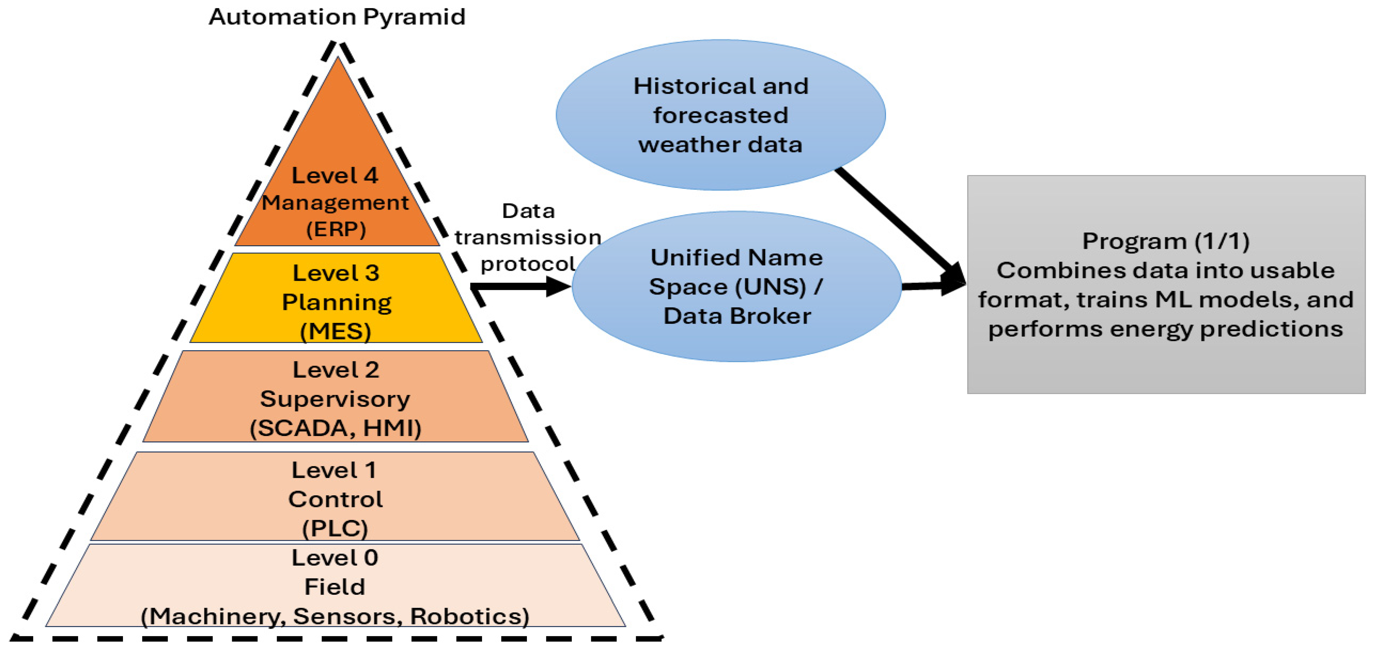
3.1. Framework Overview

Figure 1 provides a high-level framework for predicting energy consumption. Program #1 integrates data into a usable format for ML models based on historical energy consumption, weather, and production data. The output of Program #1 is a formatted dataset, along with an initial variable analysis of each data source and scatter plots of energy versus production and energy versus temperature. Program #2 uses that formatted dataset to train ML models. Program #2 output is the ML models plus model info, including coefficients, best tuning parameters, and training and holdout results such as the RMSE and R 2 and their standard deviations. Program #3 uses the created ML models with planned production data and forecasted weather data to predict energy consumption. The output of Program #3 is a dataset of each of the model’s predictions and calculations of the RMSE and R 2 if the actual data is available.
This framework could be employed at different time scales and scopes, such as at the area or line level. In our case, we use 15 min energy consumption data and daily weather and production data at the facility level. The electric vehicle manufacturing case described in this paper includes data from five shops: Assembly, Battery, Body Shop (Electric), Body Shop (Gas), and Paint. Sitewide energy is expressed as Assembly + Battery + Body Shop (Electric) + Body Shop (Gas) + Paint. We received 15 min energy data from the utility provider at the end of every week, but this data could be automatically integrated into a communication architecture.
Weather impacts manufacturing energy consumption, and weather data is available from many sources. Ref. [39] demonstrated that an online web services tool can automatically retrieve and preprocess precipitation data. An Application Programming Interface (API) like DegreeDays.net version 1.4 developed by BizEE Software could be implemented to automate this data retrieval [40].
Energy consumption heavily depends on production volumes. In this case, weekly production data is compiled into daily and monthly datasets for Assembly, Battery, Body Shops, Paint, and Sitewide. Production data will likely be the most challenging automated data collection implementation for this framework.
The ML model training can be performed through an open-source and free statistical environment such as R-4.5.1 [41]. In this environment, packages such as Caret can be utilized to develop machine learning models quickly [42]. A thorough overview of statistical learning using R-4.5.1 is provided by [43].

3.2. Prediction Models

This section provides explanations of the prediction models. We chose these well-known models because they can be roughly sorted from simple to complex, according to a review of ML models for predictive process monitoring [44]. Their parameters are explained in more detail in [45]. Chosen models include:
  • Naïve (Average)—A naïve model does not use sophisticated methods to make a prediction and is often used as a benchmark for testing ML models. An average naïve model takes the average of the training dataset and applies it to all future forecasts. If a model cannot achieve a lower root mean square error (RMSE) than the naïve model, it is not as good as random chance. The R 2 of an average naïve model is 0.
  • Naïve (Historical)—A historical naïve model takes data from one year prior and applies it to the future forecast. This is an industry practice that often improves upon the naïve average method.
  • Linear—A simple linear regression model involving only one variable, in this case, production. The equation for a line of best fit is y = m x + b , where ( x , y ) represents any point that satisfies the equation. The y -intercept, b , is the y -value when x = 0 . The slope, m, is the change in y when x increases by 1.
  • GLMNET (Net Regularized Generalized Linear Regression Model)—Considers all variables and gives a reasonable estimation of the significant predictors. It fits lasso and elastic-net models for linear, logistic, and multinomial regression using coordinate descent. It is extremely fast and exploits sparsity in the input x matrix, and can make various predictions accurately. For an alpha = 0, ridge regression is employed, which tends to yield equal coefficients and never fully eliminates predictors. For an alpha = 1, lasso regression picks fewer correlated predictors and discards the rest. For values between 0 and 1, the two methods are blended. A Generalized Linear Model (GLM) was also performed, but the results were close to GLMNET, and we chose not to include them.
  • PCR (Principal Component Regression)—In PCR, principal component analysis is first performed on the original data, then dimension reduction is accomplished by selecting the number of principal components using cross-validation and test error, and finally, regression is conducted using the first n dimension reduced principal components. PCR performs better than previous models on massive datasets and can accurately handle variables like “day of the week” and “month of the year.” Partial Least Squares Regression (PLSR) was also performed in this study, but the results were close to PCR, and we chose not to include them.
  • KNN (K-Nearest Neighbor)—A non-parametric, supervised learning classification model that uses proximity to make classifications or predictions about the grouping of an individual data point. It is typically used as a classification algorithm for pattern recognition, working off the assumption that similar points can be found near one another. It can sometimes perform better on large datasets than previous models if there is an understanding to be developed based on neighborhoods or groupings that simple linear regression cannot determine.
  • Random Forest (RF)—Random Forest is a popular ML algorithm that combines the output of decision trees to reach a result. It is popular due to its ease of use, flexibility, and ability to handle classification and regression problems.
  • Bayesian Regularized Neural Net (BRNN)—A neural network that incorporates posterior inference to reduce overfitting and can be trained based on just one parameter, the number of neurons.

3.3. Determining the Best Model

To determine the best model, we used the R 2 and RMSE metrics to compare them. R 2 is a “goodness-of-fit” statistical measure representing the proportion of the variance for a dependent variable explained by an independent variable in a regression model. The higher the R 2 value, the stronger the relationship between the dependent and independent variables. If the R 2 of a model is 0.5, then approximately half of the observed variation can be explained by the model’s inputs. What qualifies an R 2 value as “good” depends on context. Naïve (average) models have an R 2 value of 0 associated with them because they have no variance. The root mean square error (RMSE) is the standard deviation of the residuals (prediction errors). Residuals measure the distance between data points and the regression line. Essentially, the RMSE tells you how concentrated data is around the line of best fit. The lower the RMSE, the better a given model can “fit” a dataset.
Generally, the RMSE should be prioritized over R 2 in model selection because having a smaller error is preferable to having the right shape. This is apparent in several of the naïve historical models, where a high R 2 is calculated because the shape is correct, but a large RMSE exists because production has increased. In parameter selection, strict requirements for R 2 are appropriate, such that 0.85 or higher is required, but for model selection, lower R 2 can sometimes be appropriate if the RMSE is a small percentage of the total.
A general rule of thumb is that, given the choice between two equally fitting models (i.e., all else being equal), it is generally advisable to select the simpler or more parsimonious model. This principle aligns with the parsimony criterion in model selection, also known as Occam’s razor, which suggests that simpler models should be preferred when their predictive accuracy does not significantly surpass that of more complex alternatives. In general, model parsimony is a function of the number of estimated parameters and other factors, including model configuration [46]. The models in Section 3.2 are organized in roughly increasing complexity, but a detailed parsimony analysis is outside the scope of this research. The results section will highlight the model in each case with the highest R 2 and lowest RMSE, but no specific model is selected as the “best” because that is context-based.

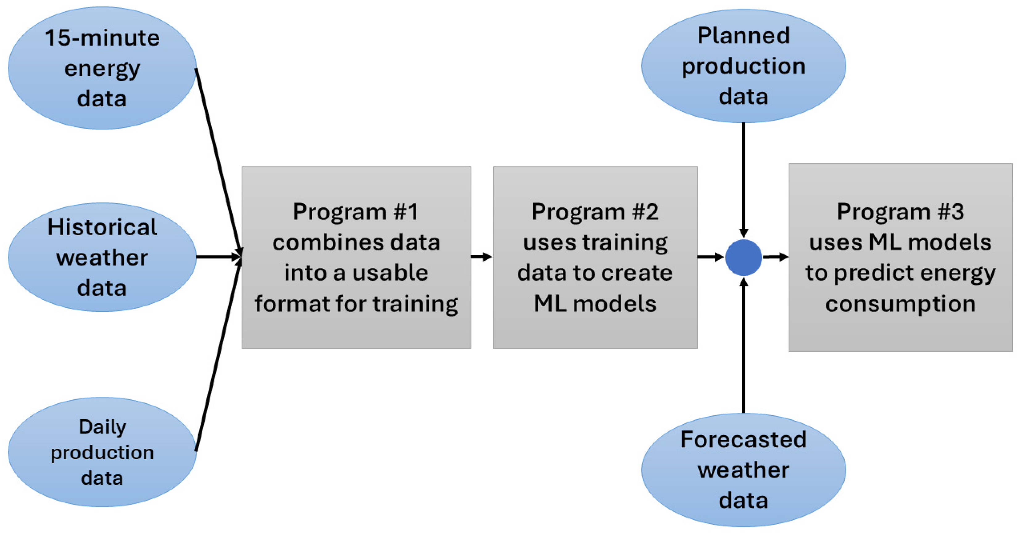
3.4. Experimental Processes

Initial variable testing was performed for dry bulb temperature, heating degree days, and cooling degree days. The decision to only include average dry bulb temperature was made to simplify the models. Heating and cooling degree days are helpful in many energy management processes, but here, when included as a predictor, it was unclear which variable would end up in the model parameters. Also, predicting heating and cooling degree days is not as straightforward as predicting dry bulb temperature. Dry bulb temperature is used as a predictor for weather in all models besides naïve and linear. From here on, the term “temperature” refers to the average dry bulb temperature.
Production and temperature are used in every model except the linear model, which only uses production, and naïve historic and average models, which do not use either. Week of the year, month, and day of the week were included in PCR, KNN, RF, and BRNN models unless the program gave an error stating that the predictors were rank-deficient, meaning they did not contribute to the model’s accuracy. Time periods with a “B” signify that an additional predictor, “Energy Data from Last Year”, is added. Including this predictor reduces the dataset size because, for 2023, we did not have energy data from the previous year. A summary of the predictors used by the model is given in Table 1.
For the shop-level models, the predictors include production data, temperature, month, week of the year (for weekly and daily models), and day of the week (for daily models). For the sitewide models, the predictors include production data for each shop and sitewide, temperature, month, week of the year for daily and weekly models, and day of the week for daily models. Month and week of the year were almost always excluded, but the day of the week was included in most daily models. A summary of the predictors used by the shop area is given in Table 2.
The weekly and daily models were cross-validated ten times, while the monthly models had three cross-validations. Because the monthly models only have 12 data points per year, many complex monthly models struggle initially due to smaller dataset. The RF would not function for any monthly sitewide models except in scenarios where we had more than two years of data. For this reason, it is not included in the monthly sitewide analysis. Because of the limited cross-validation, the data confidence for the monthly models is low. The data was randomly partitioned into 75% training and 25% holdout to ensure best practices, but holdout results are not included here.
For the results labeled 2023 Q1, data was collected from 2022 and then tested against the first quarter of 2023. For 2023 Q4 A, training data are from 2022 and 2023 up to 1 September 2023, and tested in the last quarter of 2023. For 2024 Q1 A, training data is from 2022 and 2023 and tested in the first quarter of 2024. For 2023 Q4 B and 2024 Q1 B, we included energy data from the previous year as a predictor. This reduced the size of the training dataset because we lacked data from 2021. For 2023 Q4 B, the training data is from 2023 up to 1 September 2023, and does not include any training data from 2022 because the energy from last year’s predictor does not have data from 2021. For 2024 Q1 B, training data is from 2023 and tested against the first quarter of 2024. The monthly and weekly models would not perform when we first tested in 2022 Q4, so you must have at least one year of data to perform this analysis.

4. Results

This section presents the daily, weekly, and monthly prediction results for sitewide energy, along with the energy prediction performance for each shop.

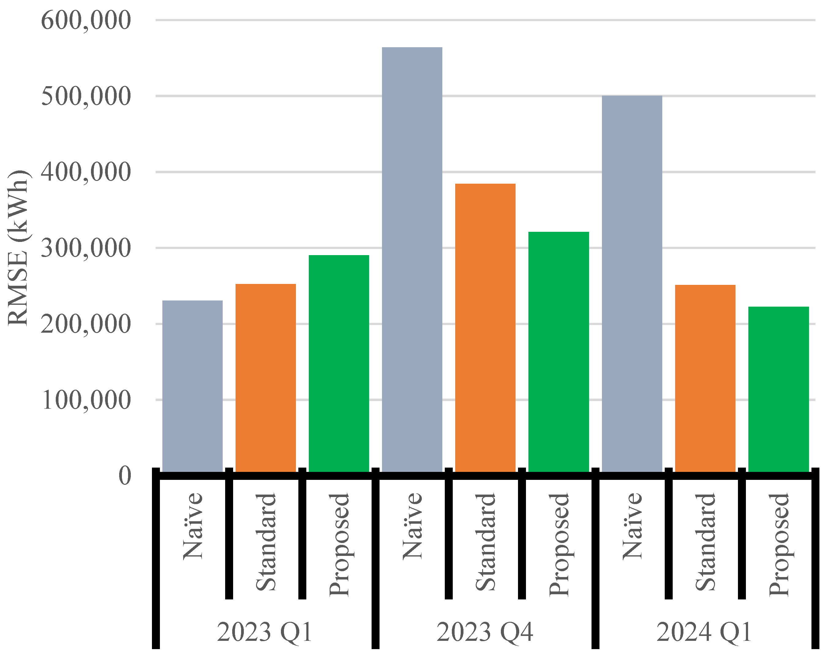
4.1. Sitewide Energy Prediction

The sitewide energy metric is derived from the readings of six different shop meters. Some significant processes, equipment, and even whole shops were added between 2022 and 2023. Production and/or temperature are used in every model except naïve historic and average models. The accuracy of their predictions is included in Appendix A.
Table 3, Table 4 and Table 5 present the sitewide energy prediction results at the daily, weekly, and monthly frequencies. In each table, the unit for energy consumption prediction RMSE is kWh. The Historic 2023 Q1 training parameters do not exist because training data was not available to compare against from 2022. “Training” refers to the model’s accuracy against the training dataset, calculated through cross-validation. “Actual” signifies the prediction accuracy in comparison with real values that were collected after model training. “B” signifies that the “Energy Data from Last Year” predictor is included, while “A” signifies that it is not. Figure 2, Figure 3, Figure 4 and Figure 5 graphically summarize the results from Table 3, Table 4 and Table 5. In these figures, the Naïve models include historical and average, the Standard models include linear and GLM without the “Energy Data from Last Year” predictor, and the Proposed models include PCR, KNN, RF, and BRNN with and without the “Energy Data from Last Year” predictor.
Daily sitewide results are given in Table 3. The average sitewide daily energy consumption was 363,040 kWh, and the RMSE standard deviation was around 5000 kWh. Prediction accuracy was above 0.85 R 2 in 2023 Q1, less than 0.05 in 2023 Q4, and greater than 0.75 R 2 in 2024 Q1. This result also played out in the assembly and paint processes and is assumed to result from low production prediction accuracy for 2023 Q4. Adding the energy data from one year ago as a predictor, shown in 2023 Q4 B and 2024 Q1 B, improved the prediction accuracy. The ML models improved on the naïve results in 2023 Q1 and 2024 Q1 but not in the 2023 Q4 analyses. In these results tables, the yellow cell fill color indicates the lowest RMSE model when compared against actual data, and the orange cell fill color indicates the highest R 2 model.
The results from Table 3 are graphically summarized in Figure 2, which demonstrates the possible value of the proposed method and the poor performance in 2023 Q4.
Table 4 shows weekly sitewide results. The average weekly energy consumption was 2,355,600 kWh, and the standard deviation of the RMSE was around 90,000. Prediction accuracy was not as bad in 2023 Q4 as in other models. As in previous models, the RMSE decreased from 2023 Q1 to 2023 Q4 and increased from 2023 Q4 to 2024 Q1, but not as severely. Comparing 2023 Q4 A with 2023 Q4 B shows that prediction accuracy did not improve based on the actual or training results from adding the energy data from the previous year’s predictor. The RMSE of the Historic model in 2023 Q1 was very good and could not be achieved, but the ML models improved upon the linear model during that period. The ML models improved on the naïve models in all other time periods. In 2024 Q1 A and B, the ML models beat the linear model only once. The sitewide model uses more predictors because it includes production data from each shop. This seems to translate to improved prediction accuracy, especially in training. In 2023 Q1, the prediction accuracy was several standard deviations better than the naïve and linear models. The sitewide weekly ML models could be used for annual predictions, such as those required for ISO 50001. These results show that the naïve and linear models can have large and unpredictable errors.
In order to demonstrate the value of the Proposed method, Figure 3 highlights the best performing weekly models according to time period and their model type. The existing commercial and research model does not allow for weekly time period predictions, but we consider linear and GLM models as the Standard for comparison purposes.
Sitewide monthly model results are given in Table 5. This is the time period that the industry typically performs yearly predictions for ISO 50001 certification. The average sitewide monthly energy consumption was 11,012,000 kWh for 2023, and the standard deviation of the RMSE was 500,000. For the ML models, prediction accuracy compared to actual results decreased from 2023 Q1 to 2023 Q4 and increased from 2023 Q4 to 2024 Q1. Prediction accuracy was not as terrible in 2023 Q4 compared to other time periods, with an R 2 above 0.75 and an RMSE less than 15% of the average monthly energy consumption. The ML models improved on the naïve models in every period besides 2023 Q1, and the linear besides 2024 Q1 A. The RF model ran in 2024 Q1 A for the first time in a monthly model, but it was the worst-performing model, and the results are not included. RF is not a good candidate for initial ML testing in monthly models because it takes more than two years of available data to perform. The BRNN did perform in 2024 Q1 B because it had a higher dimensionality with all the individual shop production data plus the “energy from last year” predictor, and it had the best prediction by the RMSE.
The RMSE of the best-performing monthly models from Table 5 are given in Figure 4. The purpose of including this comparison is to highlight the value of the proposed method. The best method depends on context, but this shows that the process of comparing different models will bring you to the best result. In 2024 Q1, the Proposed method more than halved the standard error compared to Standard and Naïve.

4.2. Shop-Level Energy Prediction

The best prediction models vary across prediction frequencies and shops. Table 6 summarizes the most accurate models and their R 2 for each shop and prediction frequency. The “best model” is chosen based on the lowest RMSE against the actual data because this indicates the model with the lowest expected error. It might be the case that another model besides the one we chose as the “best model” had a higher R 2 . Battery and Body (Electric) shops had just come online in 2023 Q1, so there are no predictions. Models with a (B) indicate the “Energy Data from Last Year” predictor was included. The monthly models in 2023 Q4 did not work with the “Energy Data from Last Year” predictor because there was not enough training data. Out of the 48 best models, 4 were Historic, 1 was Average, 10 were Linear, 5 were GLMNET, 6 were PCR, 5 were RF, 7 were KNN, and 10 were BRNN. The strongest evidence that complex models can outperform simple models is in Sitewide 2024 Q1 where the BRNN model performed two standard deviations better than the linear or naïve ones. Historical models only performed well when there was not much data available, and energy ended up being very similar to the year before, even though production was predicted to change. Of the 30 models where the “Energy Data from Last Year” predictor could be included, there were 17 times where the best model included the predictor. The monthly models had the highest R 2 , but there were instances such as Paint 2023 Q4 and Sitewide 2023 Q4 where the weekly models performed better than the monthly.

5. Discussion

5.1. Framework

Figure 5 shows an ideal application of the framework proposed in Figure 1. In this case, internal data, such as production history and production predictions, is automatically acquired, organized, and stored within a unified namespace (UNS), allowing access to data anywhere it is needed through a common data interface. David et al. [47] present the unified namespace architecture concept for integrating business data. Outside data, such as weather, is automatically acquired through HTTP/API.
Figure 5. Ideal situation of the energy prediction framework.
Energies 18 03242 g005
With good production data, the framework can be applied at various levels within the plant. For example, it could be applied at the area, line, or cell level, given that all equipment has good data. In these scenarios, temperature may or may not be a significant predictor, but others may reveal themselves through further research.

5.2. Challenges

Accurate production data and production predictions constitute a significant challenge. At one point, production data was provided in a different format with values that differed from those previously received. We determined that the reason was that one dataset was from the production line, and the other was derived. Production data must be consistently formatted, reliable, and of high quality. Also, production prediction accuracy was much better at the beginning of the year than in the last quarter. This result suggests that energy managers should exercise caution when predicting production.
Energy data quality and reliability were two more challenges in implementing this research. There were several occasions when data was unavailable when expected, or there were small gaps that had to be filled by the researchers. The utility quickly fixed these gaps, which might have prevented a real-time energy digital twin from functioning. The manufacturer’s capability to receive automated energy data weekly and view it in real-time on a shop level was excellent and bodes well for the future of energy data in manufacturing. However, it needs work to be more reliable.
Another challenge was the amount of human labor involved. This research aimed to reduce the human input needed in energy prediction. However, automating the data retrieval, ML model training, and prediction resulting in a facility-level EDT requires many human hours. The following list details the tasks that need to be automated for the automated energy prediction framework:
  • Data transmission and retrieval
  • Data formatting
  • ML model training and retraining
  • Energy consumption predictions
One reason for the large amount of human labor was that we tested several ML models. Research is needed to determine which ML model will work best for your application. In our case, we could not find any study that had implemented an ML model to predict energy consumption in the industrial sector at the plant level. The authors knew from personal experience that manufacturers use historic or average naïve models in many cases and sometimes use basic linear regression with production or multiple linear regression with production and temperature, but we had not seen any cases of using a more complex ML model. In the future, the RF will be our first candidate for removal from this process, especially for the monthly models, though it seems to perform well for the daily paint models. The next candidate would be GLM because the GLMNET is similar and improved upon the GLM in almost every model. PCR and PLSR would be our next candidates for removal from the process because they were not the best performing.
The amount of machine learning knowledge required could be challenging for real-world applications. The practitioner needs a fundamental understanding of automated data retrieval, machine learning model selection, tuning parameters, and what the results mean for energy management.

5.3. Lessons Learned

In some situations, historic and average models perform well, mainly when the system is steady, no new processes or equipment are added, and production is stable. Table 5 shows a case where historic and average models have high and low prediction errors. The problem is that there is no confidence in your prediction. Manufacturers that rely on historic and average models for predictions typically do not follow good data science practices, such as maintaining a holdout dataset or testing variables. The historic and average models are sometimes necessary for a quick estimate but can easily be improved. Manufacturers might view energy consumption prediction for energy management as unimportant and want to make the quickest estimate. The authors urge the industry to consider this a chance to improve SM capability and inform predictions.
Daily models benefit from abundant data and performed well in 2023 Q1, with R 2 above 0.7. However, their performance decreased significantly in 2023 Q4 to the point of having R 2 approaching zero. This is likely because production prediction accuracy decreases with a more extended forecast period. Also, daily datasets were derived from the weekly data provided, and if there was a shutdown or missed production target, that production was shifted to the next day. To make a good prediction, you should first have good data to input. The daily model’s application in practice will not be the same as in this research, over months or years, but rather testing for a specific scenario of a day or week. Still, the daily model results show that more flexible ML models are available with more data. One strength of the daily models is that the more complex models can run with less than a year of data.
The BRNN has high complexity and promising initial results. It works with smaller datasets than the RF or KNN. We chose the BRNN model because, compared to other neural net models, it requires less tuning. It worked well with the sitewide models with many predictors but was also the best-performing of several shop models. The KNN also had promising initial results in many of the models.

6. Conclusions

This paper proposes an energy prediction framework supported by automated data collection and machine learning (ML) models. The framework was developed at the industrial facility level, with much less existing facility energy prediction research than in the commercial sector. The novelty of this framework lies in its combination of data collection and integration for smaller-time-period energy predictions, as well as its automation of a process outlined in the ISO 50001 standard. The framework’s ability to provide near-real-time and accurate energy predictions can help manufacturers identify energy-saving opportunities, gain a deeper understanding of their processes, and make informed, data-driven decisions.
The proposed framework and research advance the state of the art in energy management. It enables manufacturers to move beyond the limitations of traditional energy management processes, which rely on inconsistent human input and do not perform energy variable analysis, and move into smart manufacturing capabilities, such as Energy Digital Twin (EDT), through automated data collection and integration into a digital model. The current state-of-the-art energy prediction research does not consider artificial intelligence prediction models or smaller time-period predictions. This study investigated more sophisticated models, including principal component reduction (PCR), K-Nearest Neighbor (KNN), Random Forest (RF), and Bayesian Regularized Neural Net (BRNN). The framework’s simplicity and adaptability allow it to be applied to various manufacturing processes and industries. A requirement of the framework is accurate and available production data and predictions. The framework was tested by performing energy consumption predictions in a large automotive original equipment manufacturer using daily, weekly, and monthly datasets for specific automotive shops and sitewide.
The results proved that ML models could be applied to industrial facility-level energy predictions at weekly and daily time scales. Complex models, such as random forest and principal component regression, were sometimes, but not always, more accurate than simpler models, such as naïve approximation and linear regression. Naïve models, which have no predictor and assume that what happened in a previous time period will happen again, do not provide confidence and should be avoided as the sole prediction method, even though they sometimes provide accurate estimates. Instead, variable analysis should be performed to identify relevant predictors and to understand what drives energy consumption. The research tested “meta” variables such as the day of the week, week of the year, month, and energy data from the previous year and found that including them often increased prediction accuracy. The major challenges identified include collecting reliable, high-quality energy and production data and the required ML expertise.
For manufacturers, the effort is better spent improving data quality and reliability, performing variable analysis, and automating the data collection framework than optimizing model selection. For future research, the authors recommend investigating different artificial intelligence methods in larger datasets, implementing the automated data collection framework, developing use cases besides ISO 50001 certification, and testing other predictors besides production, dry bulb temperature, week of the year, month, and day of the week. A sensitivity analysis of temperature prediction should also be considered. The authors used the historical average for temperature to make predictions, but this does not consider extreme weather, so different prediction sets could be developed for extreme weather.

Author Contributions

Conceptualization, D.V. and M.J.; methodology, D.V. and M.J.; validation, D.V.; formal analysis, D.V.; investigation, D.V.; resources, M.J.; data curation, D.V.; writing—original draft preparation, D.V.; writing—review and editing, M.J., T.W., and C.P.; supervision, M.J. and S.N.; project administration, M.J.; funding acquisition, T.W. and S.N. All authors have read and agreed to the published version of the manuscript.

Funding

This research was funded by the U.S. Department of Energy through Oak Ridge National Lab, project number PR12643.

Data Availability Statement

The original contributions presented in the study are included in the article, further inquiries can be directed to the corresponding author.

Conflicts of Interest

The authors declare no conflicts of interest.

Appendix A. Production and Temperature Prediction

Appendix A.1. Production Prediction

Table A1 gives the production prediction’s R 2 , which measures how accurate the partner manufacturer’s forecasts for production were. The projections were conducted at the beginning of each year, so there was a larger period between the 2023 Q4 predictions than the 2023 Q1 and 2024 Q1. Monthly and weekly production estimates were much more accurate than daily, which makes sense because the daily forecasts were derived. Daily production is more volatile due to many factors, such as maintenance, shift change, and weather. In addition, the company might miss daily goals but would make up for them through overtime on the weekend to still meet weekly and monthly goals.
Table A1. Summary of production prediction accuracy.
ShopPeriod2023 Q1
R 2
2023 Q4
R 2
2024 Q1
R 2
AssemblyDaily0.920.030.91
Weekly0.880.520.98
Monthly1.000.041.00
BatteryDaily0.960.070.69
Weekly0.880.080.88
Monthly1.000.000.94
Body
(Electric)
Daily0.800.060.60
Weekly0.760.280.52
Monthly1.000.020.74
Body
(Gas)
Daily0.880.030.85
Weekly0.740.320.97
Monthly1.000.001.00
PaintDaily0.910.020.90
Weekly0.880.520.97
Monthly1.000.051.00
SitewideDaily0.920.030.91
Weekly0.860.530.96
Monthly1.000.060.99

Appendix A.2. Temperature Prediction

Table A2 gives the temperature prediction’s R 2 , which measures how accurate our forecasts for temperature were. We used the historical averages from NCEI U.S. Daily Climate Normals (2006–2020) closest to the partner companies’ location to forecast future temperatures [48]. For monthly data, the R 2 values are high enough to use for predictions comfortably. However, there are low R 2 values for some daily and weekly predictions, so it is up to data scientists running the models to determine if it is appropriate. This study assumes that the temperature prediction accuracy did not significantly affect energy consumption prediction accuracy because the RMSE is small, and the temperature predictor importance was less than 20%.
Table A2. Summary of temperature prediction accuracy.
Period2023 Q1
R 2
2023 Q4
R 2
2024 Q1
R 2
Daily0.260.830.42
Weekly0.500.920.62
Monthly0.920.990.86

Appendix B. Assembly and Painting Shop Energy Prediction

The assembly process is more hand-tool-driven than robotics. No significant equipment changes occurred between 2022 and 2023, but production increased, particularly, the electric vehicle line. The daily results of the assembly process are given in Table A3. The average daily energy consumption was 58,600 kWh, and the standard deviation of the RMSE was ~1,000. Prediction accuracy decreased from 2023 Q4 to 2023 Q1 and improved for 2024 Q1. Prediction accuracy decreased when comparing Daily 2023 Q4 and Daily 2024 Q1 A and B, where B uses the energy data from one year ago as a predictor. The ML models were able to improve on the naïve models but could not improve on the linear model in 2023 Q1 or 2024 Q1.
Table A4 shows the weekly results of the assembly process. The average weekly energy consumption of the assembly shop was 408,000 kWh in 2023, and the standard deviation of the RMSE was about 13,000 kWh. Prediction accuracy decreased from 2023 Q4 to 2023 Q1, though not as severely as in Table A1 for daily prediction, and then improved for 2024 Q1. Adding the data from one year prior as a predictor in 2023 Q4 improved the training performance but had mixed results when used for prediction. The ML models improved on the naïve and linear models in 2023 Q1 and 2023 Q4 but not in 2024 Q1.
Table A3. Results of daily assembly shop model training.
Time
Period
ParameterModel Type
HistoricAverageLinearGLMNETPCRKNNRFBRNN
2023 Q1RMSE (Training) 15,312765747334775992011,2664534
R 2 (Training) 0.000.760.910.910.730.890.91
RMSE (Actual)16,08013,19173007627767910,65996177834
R 2 (Actual)0.730.000.830.850.850.790.860.83
2023 Q4
A
RMSE (Training)17,40915,396796557835756726057346220
R 2 (Training)0.240.000.730.860.860.780.870.83
RMSE (Actual)16,43619,47224,41118,63318,60814,53818,75723,882
R 2 (Actual)0.390.000.000.090.090.360.080.00
2023 Q4
B
RMSE (Training)17,40915,396796560014780629842673897
R 2 (Training)0.240.000.730.840.900.800.930.93
RMSE (Actual)16,43619,47224,41121,82221,27113,97218,95023,251
R 2 (Actual)0.390.000.000.020.010.400.080.01
2024
Q1
A
RMSE (Training)16,98815,9089575674010,35613,89384716568
R 2 (Training)0.320.000.630.830.610.400.840.84
RMSE (Actual)20,12016,804832110,04413,69219,67214,1929985
R 2 (Actual)0.030.000.770.810.640.610.780.81
2024
Q1
B
RMSE (Training)16,98815,908957553025263757346594923
R 2 (Training)0.320.000.630.890.890.800.920.91
RMSE (Actual)20,12016,80483218441834112,43892499355
R 2 (Actual)0.030.000.770.810.810.700.850.84
Table A4. Results of weekly assembly shop model training.
Time PeriodParameterModel Type
HistoricAverageLinearGLMNETPCRKNNRFBRNN
2023
Q1
RMSE (Training) 52,18235,36633,47230,21126,82032,92324,567
R 2 (Training) 0.000.660.700.660.740.750.67
RMSE (Actual)75,22034,29731,96821,60927,23234,45131,69236,957
R 2 (Actual)0.180.000.350.420.450.120.280.09
2023
Q4
A
RMSE (Training)78,09656,15038,93232,24433,71829,43331,98631,164
R 2 (Training)0.210.000.450.690.640.730.730.71
RMSE (Actual)75,803103,92483,73370,47468,69373,89570,56767,713
R 2 (Actual)0.670.000.230.700.720.630.780.79
2023
Q4
B
RMSE (Training)78,09656,15038,93229,43529,51528,28036,52624,926
R 2 (Training)0.210.000.450.930.930.890.420.72
RMSE (Actual)75,803103,92483,73361,22357,41674,22083,15049,462
R 2 (Actual)0.670.000.230.720.730.660.610.78
2024
Q1
A
RMSE (Training)77,13466,62357,63533,17032,77430,51234,02432,100
R 2 (Training)0.420.000.420.710.710.800.750.76
RMSE (Actual)86,28888,00436,58768,90070,09661,07065,86450,578
R 2 (Actual)0.380.000.830.750.750.790.740.84
2024
Q1
B
RMSE (Training)77,13466,62357,63530,91030,91032,95537,38125,074
R 2 (Training)0.420.000.420.790.790.790.750.85
RMSE (Actual)86,28888,00436,58767,90574,86161,52173,19581,244
R 2 (Actual)0.380.000.830.740.740.800.590.84
Table A5 gives the monthly results of the assembly process. The average monthly energy consumption of the assembly shop was 1,750,000 kWh, and the standard deviation of the RMSE was about 100,000 kWh. Prediction accuracy decreased from 2023 Q4 to 2023 Q1 and increased to a high level in 2024 Q1. “Energy Data from Last Year” was not added as a predictor to 2023 Q4 because there was not enough training data, but it was added for 2024 Q1 B, which explains why the KNN and BRNN models did not work for 2024 Q1 B. The RF model did not work in any of the time periods. KNN became available with more than one year of data. ML models significantly improved accuracy compared to naïve and linear in 2023 Q1, insignificantly improved the RMSE in 2023 Q4, and did not improve against linear in 2024 Q1.
Table A5. Results of monthly assembly shop model training.
Time PeriodParameterModel Type
HistoricAverageLinearGLMNETPCRKNNBRNN
2023
Q1
RMSE (Training) 197,900240,919227,904199,246
R 2 (Training) 0.000.650.780.71
RMSE (Actual)309,741326,770141,55656,61455,116
R 2 (Actual)0.180.000.800.750.76
2023
Q4
RMSE (Training)245,553113,581160,298118,651113,10895,892112,953
R 2 (Training)0.850.000.770.710.730.810.49
RMSE (Actual)342,804398,250374,923338,428333,659313,087347,613
R 2 (Actual)1.000.000.150.670.610.650.71
2024
Q1
A
RMSE (Training)263,020205,093237,222121,327118,610141,539149,992
R 2 (Training)0.600.000.990.760.810.630.64
RMSE (Actual)217,806151,25859,200198,204210,728249,189206,641
R 2 (Actual)0.250.000.950.930.910.880.93
2024
Q1
B
RMSE (Training)263,020205,093237,222204,262198,608
R 2 (Training)0.600.000.991.000.99
RMSE (Actual)217,806151,25859,200108,648100,846
R 2 (Actual)0.250.000.950.940.94
The painting process is almost entirely robotic. No significant process changes occurred between 2022 and 2023, but production increased, and robotics were added. Table A6 shows the daily prediction results for the paint process. The average daily energy consumption of the paint shop was 137,000 kWh in 2023, and the standard deviation of the RMSE was about 3500 kWh. Prediction accuracy fell significantly from 2023 Q1 to 2023 Q4 but improved in 2024 Q1. The most likely cause is the larger time period between production predictions. Adding the energy data from one year ago as a predictor had mixed results when comparing Daily 2023 Q4 A with Daily 2023 Q4 B. The ML models improved on the naïve and linear in most models, but it is unclear which model will be best in advance. Comparing 2023 Q4 A and B and 2024 Q1 A and B, in this case, it is better to have fewer data points and add the “Energy Data from Last Year” predictor.
Table A6. Results of daily paint shop model training.
Time PeriodParameterModel Type
HistoricAverageLinearGLMNETPCRKNNRFBRNN
2023
Q1
RMSE (Training) 44,36819,37820,83720,38430,31416,22917,829
R 2 (Training) 0.000.800.770.780.710.870.82
RMSE (Actual)48,01738,08318,47517,08017,80423,33515,75417,468
R 2 (Actual)0.630.000.860.860.860.860.900.89
2023
Q4
A
RMSE (Training)48,95942,47419,00118,98018,81215,73122,08715,588
R 2 (Training)0.100.000.810.800.800.860.830.87
RMSE (Actual)44,07542,84960,28154,43654,81859,45941,85158,686
R 2 (Actual)0.370.000.000.010.010.020.110.00
2023
Q4
B
RMSE (Training)48,95942,47419,00116,46516,39821,84813,16015,536
R 2 (Training)0.100.000.810.820.820.650.880.83
RMSE (Actual)44,07542,84960,28158,74559,75333,82849,96655,902
R 2 (Actual)0.370.000.000.000.000.340.030.00
2024
Q1
A
RMSE (Training)46,95038,89420,46621,25821,21628,64517,08417,585
R 2 (Training)0.200.000.710.770.770.590.850.84
RMSE (Actual)51,19545,51234,24652,92452,96242,89441,67040,496
R 2 (Actual)0.040.000.500.260.260.240.300.32
2024
Q1
B
RMSE (Training)46,95038,89420,46618,43818,24720,21314,83514,810
R 2 (Training)0.200.000.710.760.760.770.840.84
RMSE (Actual)51,19545,51234,24635,67035,74438,63630,72933,414
R 2 (Actual)0.040.000.500.500.540.390.540.49
Table A7 shows the weekly results of the paint process. The average weekly energy consumption in the paint shop was 956,000 kWh, and the standard deviation of the RMSE was about 100,000 kWh. The prediction accuracy was best in 2023 Q1 according to the RMSE, decreased in 2023 Q4, and stayed about the same in 2024 Q1, though R 2 improved. The “energy data from the previous year” predictor decreased the prediction accuracy on training and actual results. The ML models nearly always improved on the naïve models, and some of the ML models improved on linear models.
Table A7. Results of weekly paint shop model training.
Time
Period
ParameterModel Type
HistoricAverageLinearGLMNETPCRKNNRFBRNN
2023
Q1
RMSE (Training) 146,52462,47561,88463,41282,61482,29164,279
R 2 (Training) 0.000.850.840.840.750.800.84
RMSE (Actual)180,142343,88879,42070,35778,67466,43166,08963,193
R 2 (Actual)0.120.000.230.240.230.250.070.14
2023
Q4
A
RMSE (Training)209,886154,55761,51962,39470,76673,95981,43258,131
R 2 (Training)0.010.000.810.810.780.750.730.82
RMSE (Actual)189,218228,054153,305151,124151,124146,692159,584138,733
R 2 (Actual)0.630.000.500.510.510.640.520.62
2023
Q4
B
RMSE (Training)209,886154,55761,51961,66561,69471,29091,60968,477
R 2 (Training)0.010.000.810.890.890.730.440.74
RMSE (Actual)189,218228,054153,305176,921176,916211,926181,527152,407
R 2 (Actual)0.630.000.500.320.320.020.410.51
2024
Q1
A
RMSE (Training)201,401169,95293,29851,99752,58262,60662,23552,162
R 2 (Training)0.170.000.880.820.820.780.800.83
RMSE (Actual)242,688261,967137,637156,351165,697125,986139,460111,233
R 2 (Actual)0.410.000.810.660.670.760.690.82
2024
Q1
B
RMSE (Training)201,401169,95293,29885,25686,346108,46595,28487,986
R 2 (Training)0.170.000.880.820.850.720.780.86
RMSE (Actual)242,688261,967137,637130,600132,931183,532168,898126,133
R 2 (Actual)0.410.000.810.780.780.780.740.89
The monthly paint process model results are given in Table A8. Prediction accuracy was fair in 2023 Q1, decreased significantly in 2023 Q4, and then was at the highest levels seen in this research for 2024 Q1. Because the historical naïve model fits the actual results’ shape but consistently predicts too low, the R 2 of the historical naïve model is better than other models, but the RMSE is not. The results show that it is possible to improve on linear and naïve predictions by using ML models.
Table A8. Results of monthly paint shop model training.
Time PeriodParameterModel Type
HistoricAverageLinearGLMNETPCRKNNBRNN
2023
Q1
RMSE (Training) 411,71187,11780,91986,222
R2 (Training)0.000.970.970.97
RMSE (Actual)746,943555,007133,179230,830179,902
R2 (Actual)0.710.000.730.680.69
2023
Q4
RMSE (Training)661,834382,636118,913131,181126,773134,763122,933
R2 (Training)0.000.000.930.950.950.790.94
RMSE (Actual)760,446607,307505,900453,618454,308402,379436,012
R2 (Actual)0.150.000.030.010.010.340.03
2024
Q1
A
RMSE (Training)704,602368,219222,89190,04690,729218,414134,467
R2 (Training)0.010.000.970.980.980.650.93
RMSE (Actual)543,199608,067311,394571,267576,672251,302500,319
R2 (Actual)0.290.001.000.650.650.800.71
2024
Q1
B
RMSE (Training)704,602368,219222,891328,567342,848
R2 (Training)0.010.000.970.970.97
RMSE (Actual)543,199608,067311,394152,201132,343
R2 (Actual)0.290.001.001.001.00

References

  1. Weinert, N.; Chiotellis, S.; Seliger, G. Methodology for Planning and Operating Energy-Efficient Production Systems. CIRP Ann. 2011, 60, 41–44. [Google Scholar] [CrossRef]
  2. Lee, D.; Cheng, C.-C. Energy Savings by Energy Management Systems: A Review. Renew. Sustain. Energy Rev. 2016, 56, 760–777. [Google Scholar] [CrossRef]
  3. Duflou, J.R.; Sutherland, J.W.; Dornfeld, D.; Herrmann, C.; Jeswiet, J.; Kara, S.; Hauschild, M.; Kellens, K. Towards Energy and Resource Efficient Manufacturing: A Processes and Systems Approach. CIRP Ann. 2012, 61, 587–609. [Google Scholar] [CrossRef]
  4. ISO 50001:2018; Energy Management Systems—Requirements with Guidance for Use. International Organization of Standardization: Geneva, Switzerland, 2018. Available online: https://web.archive.org/web/20250429212254/https://www.iso.org/standard/69426.html (accessed on 28 April 2025).
  5. DOE AMO. Energy Performance Indicator Tool. Available online: https://web.archive.org/web/20250406045512/https://www.energy.gov/eere/iedo/articles/energy-performance-indicator-tool?nrg_redirect=465586 (accessed on 28 April 2025).
  6. DOE AMO. Better Plants Software Tools. Available online: https://web.archive.org/web/20250416042229/https://betterbuildingssolutioncenter.energy.gov/better-plants/software-tools (accessed on 28 April 2025).
  7. Vance, D.; Jin, M.; Price, C.; Nimbalkar, S.U.; Wenning, T. Smart Manufacturing Maturity Models and Their Applicability: A Review. J. Manuf. Technol. Manag. 2023, 34, 735–770. [Google Scholar] [CrossRef]
  8. Narciso, D.A.C.; Martins, F.G. Application of Machine Learning Tools for Energy Efficiency in Industry: A Review. Energy Rep. 2020, 6, 1181–1199. [Google Scholar] [CrossRef]
  9. Liu, Z.; Wang, X.; Zhang, Q.; Huang, C. Empirical Mode Decomposition Based Hybrid Ensemble Model for Electrical Energy Consumption Forecasting of the Cement Grinding Process. Measurement 2019, 138, 314–324. [Google Scholar] [CrossRef]
  10. Moghadasi, M.; Izadyar, N.; Moghadasi, A.; Ghadamian, H. Applying Machine Learning Techniques to Implement the Technical Requirements of Energy Management Systems in Accordance with ISO50001:2018, An Industrial Case Study. Energy Sources Part A Recovery Util. Environ. Eff. 2021, 1–18. [Google Scholar] [CrossRef]
  11. Shrouf, F.; Ordieres, J.; Miragliotta, G. Smart Factories in Industry 4.0: A Review of the Concept and of Energy Management Approached in Production Based on the Internet of Things Paradigm. In Proceedings of the 2014 IEEE International Conference on Industrial Engineering and Engineering Management, Selangor, Malaysia, 9–12 December 2014; IEEE: Piscataway, NJ, USA, 2014; pp. 697–701. [Google Scholar] [CrossRef]
  12. Medojevic, M.; Villar, P.D.; Cosic, I.; Rikalovic, A.; Sremcev, N.; Lazarevic, M. Energy Management in Industry 4.0 Ecosystem: A Review on Possibilities and Concerns. Ann. DAAAM Proc. 2018, 29, 674–680. [Google Scholar] [CrossRef]
  13. Shrouf, F.; Miragliotta, G. Energy Management Based on Internet of Things: Practices and Framework for Adoption in Production Management. J. Clean. Prod. 2015, 100, 235–246. [Google Scholar] [CrossRef]
  14. Khan, M.; Wu, X.; Xu, X.; Dou, W. Big Data Challenges and Opportunities in the Hype of Industry 4.0. In Proceedings of the 2017 IEEE International Conference on Communications (ICC), Paris, France, 21–25 May 2017; IEEE: Piscataway, NJ, USA, 2017; pp. 1–6. [Google Scholar] [CrossRef]
  15. Sievers, J.; Blank, T. A Systematic Literature Review on Data-Driven Residential and Industrial Energy Management Systems. Energies 2023, 16, 1688. [Google Scholar] [CrossRef]
  16. May, G.; Stahl, B.; Taisch, M.; Kiritsis, D. Energy Management in Manufacturing: From Literature Review to a Conceptual Framework. J. Clean. Prod. 2017, 167, 1464–1489. [Google Scholar] [CrossRef]
  17. Pater, J.; Stadnicka, D. Towards Digital Twins Development and Implementation to Support Sustainability—Systematic Literature Review. Manag. Prod. Eng. Rev. 2021, 13, 63–73. [Google Scholar] [CrossRef]
  18. Walther, J.; Weigold, M. A Systematic Review on Predicting and Forecasting the Electrical Energy Consumption in the Manufacturing Industry. Energies 2021, 14, 968. [Google Scholar] [CrossRef]
  19. Dietmair, A.; Verl, A. A Generic Energy Consumption Model for Decision Making and Energy Efficiency Optimisation in Manufacturing. Int. J. Sustain. Eng. 2009, 2, 123–133. [Google Scholar] [CrossRef]
  20. Su, C.-L. Load Estimation in Industrial Power Systems for Expansion Planning. IEEE Trans. Ind. Appl. 2011, 47, 2311–2323. [Google Scholar] [CrossRef]
  21. Walther, J.; Spanier, D.; Panten, N.; Abele, E. Very Short-Term Load Forecasting on Factory Level–A Machine Learning Approach. Procedia CIRP 2019, 80, 705–710. [Google Scholar] [CrossRef]
  22. Mawson, V.J.; Hughes, B.R. Deep Learning Techniques for Energy Forecasting and Condition Monitoring in the Manufacturing Sector. Energy Build. 2020, 217, 109966. [Google Scholar] [CrossRef]
  23. Chen, Z.; Xiao, F.; Guo, F.; Yan, J. Interpretable Machine Learning for Building Energy Management: A State-of-the-Art Review. Adv. Appl. Energy 2023, 9, 100123. [Google Scholar] [CrossRef]
  24. Mahir, S.M.; Koch, G.; Herne, J.; Lee, J.J. Data Acquisition Platform for The Energy Management of Smart Factories and Buildings. In Proceedings of the 2023 17th International Conference on Ubiquitous Information Management and Communication (IMCOM), Seoul, Republic of Korea, 3–5 January 2023; IEEE: Piscataway, NJ, USA, 2023; pp. 1–7. [Google Scholar] [CrossRef]
  25. Weber, C.; Königsberger, J.; Kassner, L.; Mitschang, B. M2DDM—A Maturity Model for Data-Driven Manufacturing. Procedia CIRP 2017, 63, 173–178. [Google Scholar] [CrossRef]
  26. Grieves, M. Digital Twin: Manufacturing Excellence Through Virtual Factory Replication. White Pap. 2014, 1, 1–7. [Google Scholar]
  27. Glaessgen, E.; Stargel, D. The Digital Twin Paradigm for Future NASA and US Air Force vehicles. In Proceedings of the 53rd AIAA/ASME/ASCE/AHS/ASC Structures, Structural Dynamics and Materials Conference, Honolulu, HI, USA, 23–26 April 2012; p. 1818. [Google Scholar] [CrossRef]
  28. Garetti, M.; Rosa, P.; Terzi, S. Life Cycle Simulation for the Design of Product-Service Systems. Comput. Ind. 2012, 63, 361–369. [Google Scholar] [CrossRef]
  29. Kritzinger, W.; Karner, M.; Traar, G.; Jan, H.; Wilfried, S. Digital Twin in Manufacturing: A Categorical Literature Review and Classification. IFAC-Pap. 2018, 51, 1016–1022. [Google Scholar] [CrossRef]
  30. Shao, G.; Helu, M. Framework for a Digital Twin in Manufacturing: Scope and Requirements. Manuf. Lett. 2020, 24, 105–107. [Google Scholar] [CrossRef] [PubMed]
  31. Yu, W.; Patros, P.; Young, B.; Klinac, E.; Walmsley, T.G. Energy Digital Twin Technology for Industrial Energy Management: Classification, Challenges and Future. Renew. Sustain. Energy Rev. 2022, 161, 112407. [Google Scholar] [CrossRef]
  32. Haag, S.; Anderl, R. Digital twin—Proof of Concept. Manuf. Lett. 2018, 15, 64–66. [Google Scholar] [CrossRef]
  33. Tao, F.; Zhang, H.; Liu, A.; Nee, A.Y.C. Digital Twin in Industry: State-of-the-Art. IEEE Trans. Ind. Inf. 2018, 15, 2405–2415. [Google Scholar] [CrossRef]
  34. Assad, F.; Konstantinov, S.; Ahmad, M.H.; Rushforth, E.J.; Harrison, R. Utilising Web-based Digital Twin to Promote Assembly Line Sustainability. In Proceedings of the 2021 4th IEEE International Conference on Industrial Cyber-Physical Systems (ICPS), Victoria, BC, Canada, 10–12 May 2021; pp. 381–386. [Google Scholar] [CrossRef]
  35. Schulze, M.; Nehler, H.; Ottosson, M.; Thollander, P. Energy Management in Industry—A Systematic Review of Previous Findings and an Integrative Conceptual Framework. J. Clean. Prod. 2016, 112, 3692–3708. [Google Scholar] [CrossRef]
  36. Vikhorev, K.; Greenough, R.; Brown, N. An Advanced Energy Management Framework to Promote Energy Awareness. J. Clean. Prod. 2013, 43, 103–112. [Google Scholar] [CrossRef]
  37. Zhang, M.; Zuo, Y.; Tao, F. Equipment Energy Consumption Management in Digital Twin Shop-Floor: A Framework and Potential Applications. In Proceedings of the 2018 IEEE 15th International Conference on Networking, Sensing and Control (ICNSC), Zhuhai, China, 27–29 March 2018; IEEE: Piscataway, NJ, USA, 2018; pp. 1–5. [Google Scholar] [CrossRef]
  38. Wei, M.; Hong, S.H.; Alam, M. An IoT-Based Energy-Management Platform for Industrial Facilities. Appl. Energy 2016, 164, 607–619. [Google Scholar] [CrossRef]
  39. Sitterson, J.; Sinnathamby, S.; Parmar, R.; Koblich, J.; Wolfe, K.; Knightes, C.D. Demonstration of an Online Web Services Tool Incorporating Automatic Retrieval and Comparison of Precipitation Data. Environ. Model. Softw. 2020, 123, 104570. [Google Scholar] [CrossRef]
  40. BizEE Software. Degree Days Calculated Accurately for Locations Worldwide. Available online: https://web.archive.org/web/20250402181725/https://www.degreedays.net/ (accessed on 28 April 2025).
  41. R. What is R? Available online: https://web.archive.org/web/20250424231453/https://www.r-project.org/about.html (accessed on 28 April 2025).
  42. Prabhakaran, S. Caret Package—A Practical Guide to Machine Learning in R. Available online: https://web.archive.org/web/20250306212733/https://www.machinelearningplus.com/machine-learning/caret-package/ (accessed on 28 April 2025).
  43. James, G.; Witten, D.; Hastie, T.; Tibshirani, R.; Taylor, J. An Introduction to Statistical Learning; Springer Texts in Statistics; Springer International Publishing: Cham, Switzerland, 2023; Volume 112. [Google Scholar] [CrossRef]
  44. Mehdiyev, N.; Majlatow, M.; Fettke, P. Interpretable and Explainable Machine Learning Methods for Predictive Process Monitoring: A Systematic Literature Review. arXiv 2023. arXiv:2312.17584. [Google Scholar] [CrossRef]
  45. Caret Documentation. CARET: A List of Available Models in TRAIN, rdrr.io. Available online: https://web.archive.org/web/20250429202653/https://rdrr.io/cran/caret/man/models.html (accessed on 28 April 2024).
  46. Falk, C.F.; Muthukrishna, M. Parsimony in Model Selection: Tools for Assessing Fit Propensity. Psychol. Methods 2023, 28, 123–136. [Google Scholar] [CrossRef] [PubMed]
  47. David, J.; Martikkala, A.; Lobov, A.; Lanz, M. A Unified Ontology Namespace for Enterprise Integration—A Digital Twin Case Study. In Proceedings of the Instrumentation Engineering, Electronics and Telecommunications—2019, Izhevsk, Russia, 20–22 November 2019. [Google Scholar] [CrossRef]
  48. National Centers for Environmental Information. U.S. Climate Normals. Available online: https://web.archive.org/web/20250426104931/https://www.ncei.noaa.gov/products/land-based-station/us-climate-normals (accessed on 28 April 2025).
Figure 1. Framework for energy consumption prediction of a manufacturing facility.
Energies 18 03242 g001
Figure 2. RMSE of best performing daily sitewide models by model type.
Energies 18 03242 g002
Figure 3. RMSE of best performing sitewide weekly models by model type.
Energies 18 03242 g003
Figure 4. RMSE of the best performing sitewide monthly models by model type.
Energies 18 03242 g004
Table 1. Summary of predictors by model type.
ModelPredictors
HistoricA naïve model, meaning no predictors are used. The output is historical energy consumption.
AverageAnother naïve model. The output is the average of historical energy consumption.
LinearProduction
GLMNETProduction, Temperature
PCRProduction, Temperature, Day of the Week, Week of the Year, Month
KNNProduction, Temperature, Day of the Week, Week of the Year, Month
RFProduction, Temperature, Day of the Week, Week of the Year, Month
BRNNProduction, Temperature, Day of the Week, Week of the Year, Month
BAn additional predictor, “Energy Data from Last Year”, is included.
Table 2. Summary of predictors by plant area.
Plant AreaTime PeriodPredictors
AssemblyDailyAssembly Production, Temperature, Day of the Week, Week of the Year, Month
WeeklyAssembly Production, Temperature, Week of the Year
MonthlyAssembly Production, Temperature, Month
BatteryDailyBattery Production, Temperature, Day of the Week, Week of the Year, Month
WeeklyBattery Production, Temperature, Week of the Year
MonthlyBattery Production, Temperature, Month
Body
(Electric)
DailyBody (Electric) Production, Temperature, Day of the Week, Week of the Year, Month
WeeklyBody (Electric) Production, Temperature, Week of the Year
MonthlyBody (Electric) Production, Temperature, Month
Body
(Gas)
DailyBody (Gas) Production, Temperature, Day of the Week, Week of the Year, Month
WeeklyBody (Gas) Production, Temperature, Week of the Year
MonthlyBody (Gas) Production, Temperature, Week of the Year
PaintDailyPaint Production, Temperature, Day of the Week, Week of the Year, Month
WeeklyPaint Production, Temperature, Week of the Year
MonthlyPaint Production, Temperature, Week of the Year
SitewideDailyAssembly Production, Battery Production, Body (Electric) Production, Body (Gas) Production, Paint Production, Temperature, Day of the Week, Week of the Year, Month
WeeklyAssembly Production, Battery Production, Body (Electric) Production, Body (Gas) Production, Paint Production, Temperature, Week of the Year
MonthlyAssembly Production, Battery Production, Body (Electric) Production, Body (Gas) Production, Paint Production, Temperature, Month
Table 3. Results of daily sitewide model training.
PeriodParameterModel Type
HistoricAverageLinearGLMNETPCRKNNRFBRNN
2023
Q1
RMSE (Training) 105,62954,29134,98933,88145,84858,32933,456
R 2 (Training)0.000.730.890.900.880.880.91
RMSE (Actual)78,85274,088181,57754,02653,37833,07849,52431,823
R 2 (Actual)0.700.000.870.920.920.890.920.87
2023
Q4
A
RMSE (Training)113,657103,47854,35634,99034,84532,74930,35127,950
R 2 (Training)0.190.000.730.890.890.900.920.93
RMSE (Actual)112,459124,464160,524132,719135,631135,333140,233143,182
R 2 (Actual)0.440.000.000.030.020.010.010.00
2023
Q4
B
RMSE (Training)113,657101,95854,35640,69840,27436,10528,85726,677
R 2 (Training)0.190.000.730.840.840.870.910.92
RMSE (Actual)112,459120,878160,524129,048124,096131,786142,825127,605
R 2 (Actual)0.440.000.000.030.040.030.000.02
2024
Q1
A
RMSE (Training)113,028103,34568,07942,90642,83437,58030,84431,530
R 2 (Training)0.290.000.560.850.850.880.920.92
RMSE (Actual)114,349107,52458,08457,84260,11378,92867,84658,269
R 2 (Actual)0.050.000.740.780.760.650.790.79
2024
Q1
B
RMSE (Training)113,028103,34568,07939,52935,92440,25131,93933,243
R 2 (Training)0.290.000.560.850.870.860.910.89
RMSE (Actual)114,349107,52458,08452,54446,19757,92857,71156,881
R 2 (Actual)0.050.000.740.780.810.780.790.81
The Historic 2023 Q1 training parameters (signified with black background color) do not exist because no training data was available to compare against from 2022. “B” signifies that the “Energy Data from Last Year” predictor is included, while “A” signifies that it is not included.
Table 4. Results of weekly sitewide training.
PeriodParameterModel Type
HistoricAverageLinearGLMNETPCRKNNRFBRNN
2023
Q1
RMSE (Training) 456,963297,607186,355183,373160,581205,657107,720
R 2 (Training)0.000.730.840.850.790.890.95
RMSE (Actual)230,6101,806,3131,321,370252,767534,254391,638290,422350,465
R 2 (Actual)0.400.000.450.410.450.230.170.27
2023
Q4
A
RMSE (Training)507,147406,336293,128160,703160,628150,152193,71795,710
R 2 (Training)0.180.000.550.880.870.910.830.96
RMSE (Actual)564,164697,198553,789384,559384,182403,828461,169333,189
R 2 (Actual)0.670.000.210.750.740.730.630.77
2023
Q4
B
RMSE (Training)507,147406,336293,128235,608230,918242,368296,876244,444
R 2 (Training)0.180.000.550.960.960.990.250.53
RMSE (Actual)564,164697,198553,789385,571367,732540,490578,331321,153
R 2 (Actual)0.670.000.210.720.750.590.540.78
2024
Q1
A
RMSE (Training)532,016474,094419,285157,103158,933150,871173,645110,520
R 2 (Training)0.370.000.390.900.900.910.900.95
RMSE (Actual)500,572609,475251,523280,070279,656222,876273,626262,489
R 2 (Actual)0.440.000.850.770.770.830.820.83
2024
Q1
B
RMSE (Training)532,016474,094419,285201,078198,221263,295262,053184,889
R 2 (Training)0.370.000.390.870.880.870.810.95
RMSE (Actual)500,572609,475251,523322,663363,583304,783464,141424,085
R 2 (Actual)0.440.000.850.790.790.760.570.85
“B” signifies that the “Energy Data from Last Year” predictor is included, while “A” signifies that it is not included. The Historic 2023 Q1 training parameters (signified with black background color) do not exist because no training data was available to compare against from 2022.
Table 5. Results of monthly sitewide model training.
PeriodParameterModel Type
HistoricAverageLinearGLMNETPCRKNNBRNN
2023
Q1
RMSE (Training) 1,747,31131,227,409682,160737,764
R 2 (Training)0.000.660.910.92
RMSE (Actual)748,7921,445,6744,219,0153,263,4491,159,504
R 2 (Actual)0.890.000.820.120.72
2023
Q4
RMSE (Training)1,706,9151,378,8261,431,324607,102558,8041,026,0881,286,387
R 2 (Training)0.580.000.380.970.970.640.69
RMSE (Actual)2,288,1142,544,5552,272,7901,388,6371,302,0621,346,7541,212,710
R 2 (Actual)0.680.000.150.770.790.860.80
2024
Q1
A
RMSE (Training)1,970,0301,533,3101,757,608585,057606,5291,021,876567,022
R 2 (Training)0.510.000.980.960.940.740.95
RMSE (Actual)1,067,8211,625,809630,998680,560966,4461,009,443758,261
R 2 (Actual)0.510.001.000.960.950.710.97
2024
Q1
B
RMSE (Training)1,970,0301,533,3101,757,6081,024,3961,301,112 1,339,096
R 2 (Training)0.510.000.980.970.990.97
RMSE (Actual)1,067,8211,625,809630,9981,250,344428,949291,403
R 2 (Actual)0.510.001.000.990.990.96
Models with black backgrounds, including KNN and BRNN 2023 Q1 models, do not exist because of insufficient data. In 2023 Q1, with data collection starting in January 2022, there are only 12 monthly data points. The KNN model in Q1B 2024 also does not work due to insufficient data. Adding the “Energy Data from Last Year” predictor eliminates a year of data because we do not have data from a year prior.
Table 6. Summary of the best models for each shop.
Plant AreaPeriod2023 Q12023 Q42024 Q1
Best Model R 2 Best Model R 2 Best Model R 2
AssemblyDailyLinear0.83KNN (B)0.40Linear0.77
WeeklyGLMNET0.42BRNN (B)0.78Linear0.83
MonthlyPCR0.76Historical0.72Linear0.95
BatteryDaily KNN (B)0.49Linear0.42
Weekly GLMNET (B)0.72RF (B)0.58
Monthly BRNN0.78Average0
Body
(Electric)
Daily KNN (B)0.23RF (B)0.78
Weekly BRNN (A)0.77RF (A)0.81
Monthly BRNN0.85GLMNET (B)0.86
Body
(Gas)
DailyPCR0.93KNN (B)0.46GLMNET (A)0.79
WeeklyLinear0.59BRNN (B)0.69Linear0.81
MonthlyLinear0.96KNN0.66PCR (B)0.98
PaintDailyRF0.90KNN (B)0.34RF (B)0.54
WeeklyBRNN0.14BRNN (A)0.62BRNN (A)0.82
MonthlyLinear0.73KNN0.34PCR (B)1.00
SitewideDailyPCR0.92Historical0.44PCR (B)0.80
WeeklyHistorical0.40BRNN (B)0.78Linear0.85
MonthlyHistorical0.89GLMNET0.75BRNN (B)0.96
Battery and Body (Electric) came online in 2023 Q1, so there is no result for 2023 Q1. “B” signifies that the “Energy Data from Last Year” predictor is included, while “A” signifies that it is not included.
Disclaimer/Publisher’s Note: The statements, opinions and data contained in all publications are solely those of the individual author(s) and contributor(s) and not of MDPI and/or the editor(s). MDPI and/or the editor(s) disclaim responsibility for any injury to people or property resulting from any ideas, methods, instructions or products referred to in the content.

