Unequal Energy Footprints: Trade-Driven Asymmetries in Consumption-Based Carbon Emissions of the U.S. and China

Abstract

This study examines the symmetric and asymmetric impacts of international trade on consumption-based carbon emissions (CBEs) in the People’s Republic of China (PRC) and the United States of America (USA) from 1990 to 2018. The analysis uses autoregressive distributed lag (ARDL) and non-linear ARDL (NARDL) methodologies to capture short- and long-run trade emissions dynamics, with economic growth, oil prices, financial development and industry value addition as control variables. The findings reveal that exports reduce CBEs, while imports increase them, across both economies in the long and short run. The asymmetric analysis highlights that a fall in exports increases CBEs in the USA but reduces them in the PRC due to differences in supply chain flexibility. The PRC demonstrates larger coefficients for trade variables, reflecting its reliance on energy-intensive imports and rapid trade growth. The error correction term shows that the PRC takes 2.64 times longer than the USA to return to equilibrium after short-run shocks, reflecting systemic rigidity. These findings challenge the Environmental Kuznets Curve (EKC) hypothesis, showing that economic growth intensifies CBEs. Robustness checks confirm the results, highlighting the need for tailored policies, including carbon border adjustments, renewable energy integration and CBE-based accounting frameworks.

1. Introduction

Greenhouse gas emissions have increased the Earth’s temperature by 1.9 degrees Fahrenheit and the sea level by 7 inches. Researchers provide evidence that, even if all emissions are halted from today, the already stored emission levels are enough to adversely impact future life on Earth [1]. Due to the significant socioeconomic impacts of climate change, the United Nations (UN) requires countries to formulate policies to adapt to climate change’s adverse impacts while also considering steps to mitigate emission levels [2]. The United Nations currently uses territorial-based carbon emissions (TBEs) accounting to hold countries responsible for their mitigation, where such mechanisms only consider emissions produced in a country’s territory [3,4]. Such a conventional mechanism allows developed countries to comply with emissions mitigation requirements by transferring energy-intensive industries to other parts of the world, thus protecting themselves from carbon accountability [5].

This practice, known as carbon leakage, occurs when businesses relocate to other countries to cap emissions while importing the produced products [6,7,8]. Due to the apparent failure of TBEs to capture carbon leakage, consumption-based carbon emissions (CBEs) are gaining momentum, addressing this shortcoming [9,10,11,12]. CBEs account for the total emissions associated with a country’s consumption by including emissions embodied in imports and excluding those in exports. Researchers increasingly advocate for the adoption of CBEs as a more accurate framework in assigning emissions mitigation responsibilities, particularly for emissions embedded in international trade [12,13].

Numerous studies provide evidence of the relationship between trade and carbon emissions [14,15,16,17]; however, such studies primarily rely on TBEs, which overlook carbon leakage. Prior studies that have examined the relationship between trade and TBEs have largely ignored the individual impacts of imports and exports on TBEs [14,15,18]. Furthermore, CBEs also challenge the argument of emissions convergence, known as the Environmental Kuznets Curve hypothesis (EKCH), where an inverted-U-shaped relationship exists between economic growth and TBEs [19,20,21,22]. Considering the role of trade in a country’s economic growth, ignoring the emissions embodied in trade to assess the EKCH provides an over-optimistic belief that further economic growth can reduce emissions [23].

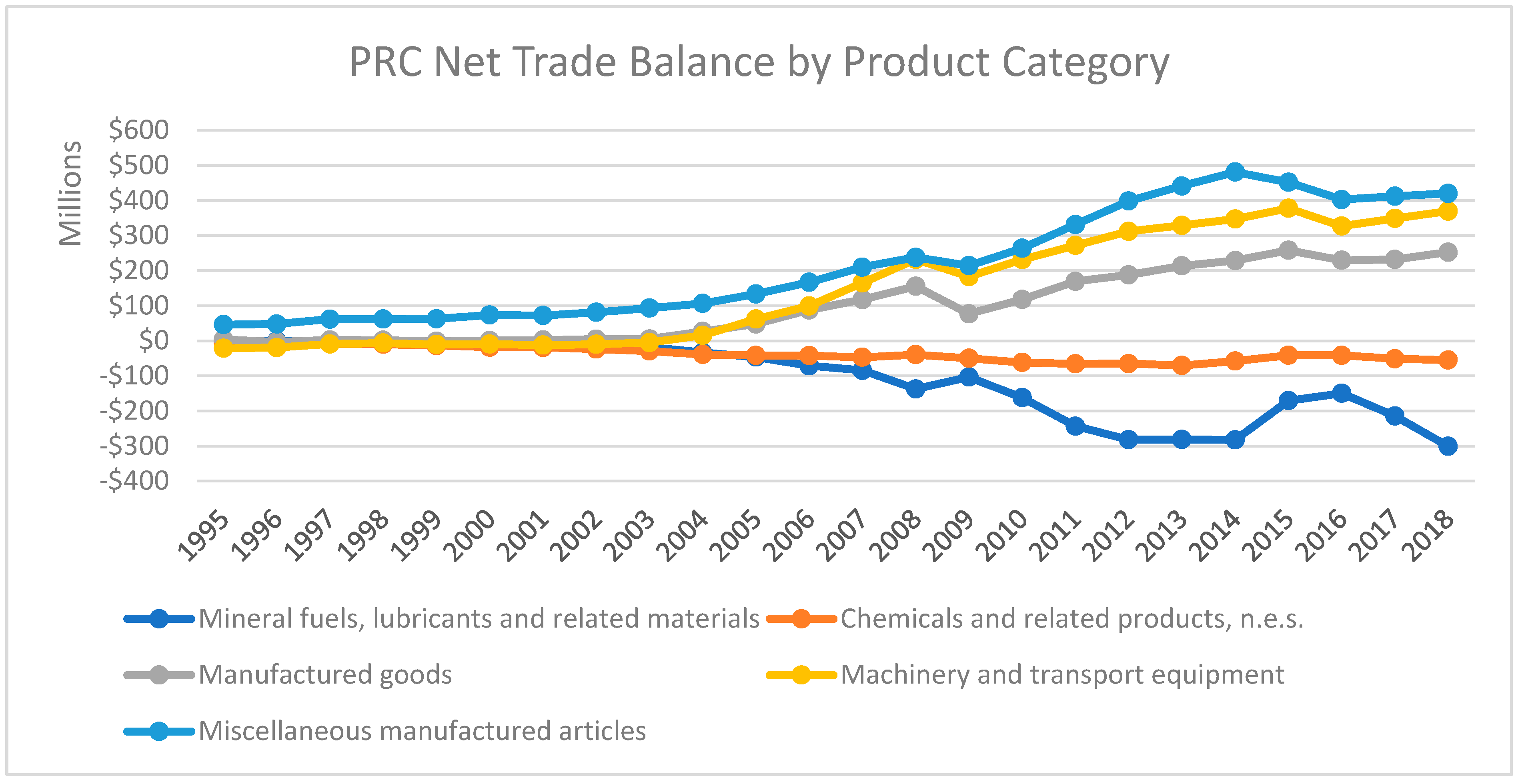
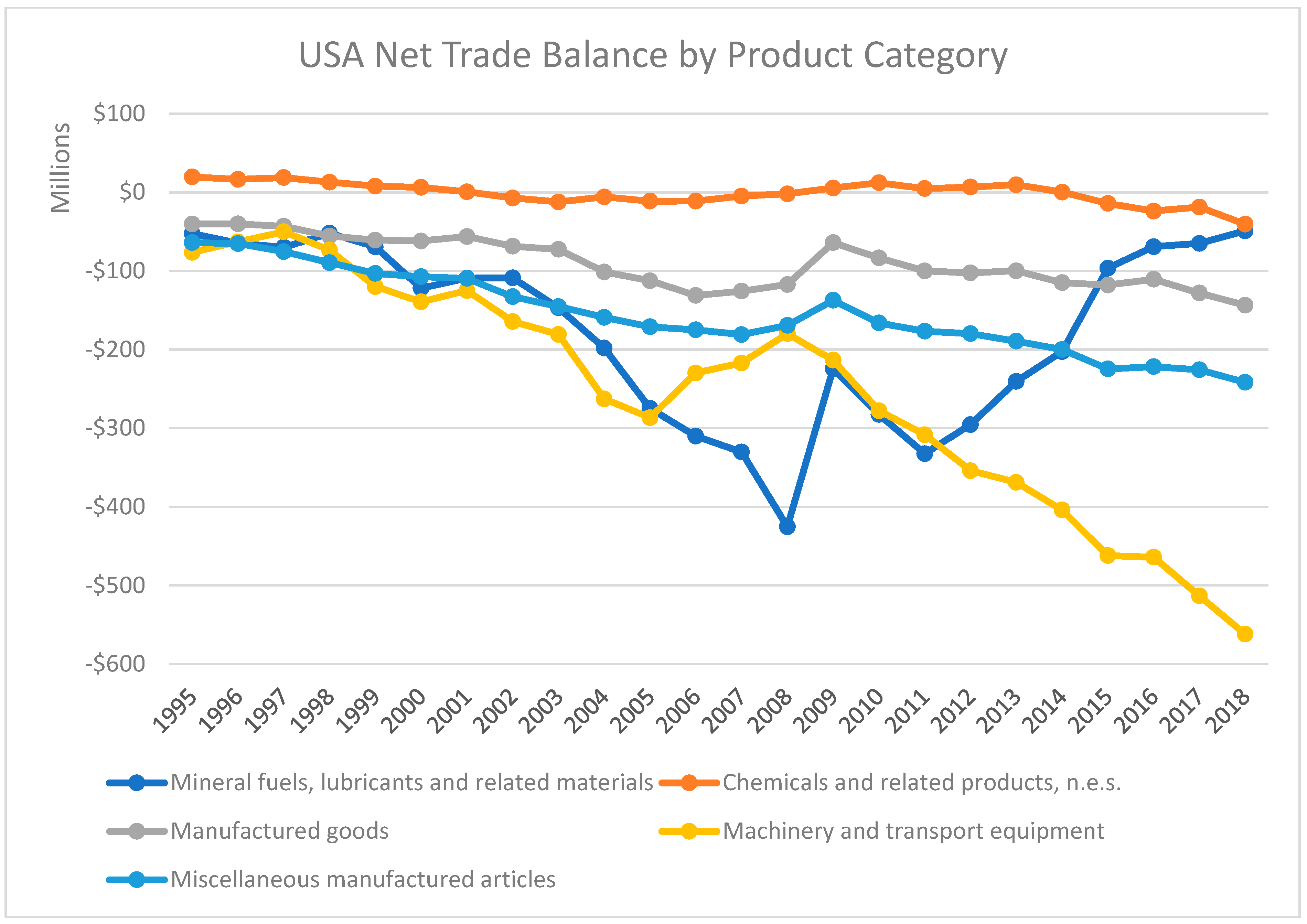
A growing number of studies are examining the individual impact of trade on CBEs. However, past studies have focused on a group of countries, like the OECD, the European Union, oil-exporting countries, or a combination of developed and developing economies [23,24,25,26], while ignoring the impact of the disaggregate level of trade for an individual country. Moreover, past studies have only examined the symmetric impact of trade on CBEs. No study has examined the asymmetric relationship between exports and imports and CBEs for an individual country. Due to this apparent gap, this study’s objective is to examine the symmetric and asymmetric impacts of the disaggregate level of trade on the CBEs of the two greatest energy consumers of the world, namely the People’s Republic of China (PRC) and the United States of America (USA).

The PRC and the USA are two major economies globally, representing 25% of global trade while holding top positions among their peer groups in trade [27]. Both these economies are the most significant consumers of energy and the greatest producers of emissions globally, where the PRC relies on coal and the USA relies on oil to fulfill its growing energy demand [28]. Although innovation has rendered the whole production process more efficient, at the same time, it has allowed countries to increase their production outputs, thus consuming more energy and producing higher emissions levels [29,30,31]. Thus, considering the sheer extent of the energy consumption and trade volumes of the PRC and the USA, they are excellent candidates to strengthen the argument for embodied emissions in trade.

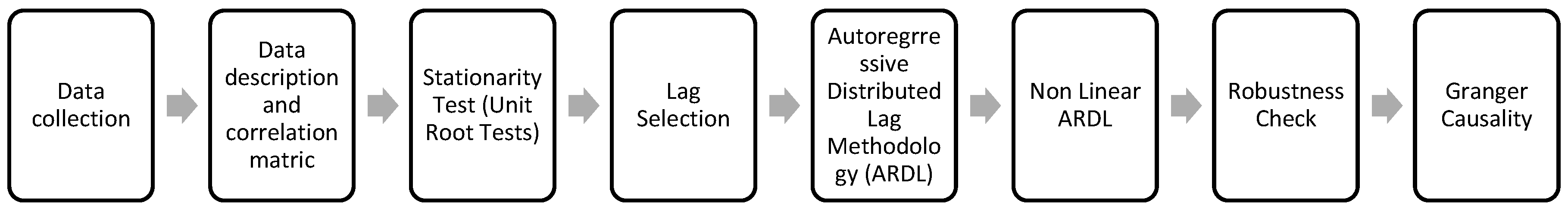
For analysis, this study considers the period from 1990 to 2018, which was selected to ensure stable trade patterns unaffected by large structural breaks. In 2019, two major disruptions emerged: the intensified US–China trade war and the global COVID-19 pandemic. Both events significantly altered trade flows and emissions patterns [32,33], introducing volatility that would compromise long-run equilibrium analysis. Therefore, this timeframe ensures consistency and robustness in the econometric modeling. This study extends the current line of literature in the following ways. Firstly, this study performs a comparative analysis by examining the long- and short-run impact of exports and imports on the CBEs of the PRC and the USA by employing the autoregressive distributed lag (ARDL) methodology. Secondly, beyond symmetric analysis, this study also explores the asymmetric impact of the disaggregate level of trade on CBEs by employing a non-linear autoregressive distributed lag (NARDL) approach, revealing nuanced dynamics in trade and emissions relationships. Thirdly, besides exports and imports, this study also examines the EKC hypothesis, highlighting its limitations when assessed using territorial-based emissions (TBEs). It underscores the importance of adopting CBEs as a more accurate metric, particularly for economies with substantial trade volumes. Control variables such as economic growth, oil prices, financial development and industry value addition are also incorporated to comprehensively analyze the factors influencing CBEs. Lastly, this study applies the dynamic ordinary least squares (DOLS) methodology for robustness analysis, while also utilizing Granger causality to assess the flow of causality among the study variables.

This study’s findings indicate that exports diminish and imports augment CBEs in both the short and long term for the PRC and the USA, with the PRC exhibiting greater coefficient magnitudes due to its accelerated trade expansion and dependence on energy-intensive imports. The findings do not corroborate the EKC theory, suggesting that economic expansion exacerbates CBEs in both economies. The findings regarding the error correction term indicate that the PRC requires a 2.64 times longer duration than the USA to achieve equilibrium after a short-run shock, highlighting systemic rigidity in its emissions systems. These findings offer new perspectives on the trade–emissions relationship, highlighting the necessity of tailored and nation-specific carbon reduction policies.

The remaining parts of this study are organized in the following manner: Section 2 discusses the literature review, while Section 3 describes the model and methodological element. Section 4 covers the results and discussion, and Section 5 provides the conclusions and policy implications.

2. Literature Review

Industrialization and globalization, supplemented by the formation of the World Trade Organization (WTO), raised international trade among countries by streamlining the overall global trade structure during the 20th century. Although the growing trade volume has enabled both developed and developing economies to enhance their economic growth, such growth has also adversely impacted the environment [34,35,36]. Multiple works of literature have examined the relationship between trade and carbon emissions, but they provide mixed findings. For instance, Shahbaz, M., S. Nasreen, K. Ahmed and S. Hammoudeh [16] investigated the impact of trade openness on the carbon emissions of 105 economies and found the relationship to be positive. Meanwhile Kim, D.-H., Y.-B. Suen and S.-C. Lin [37] studied the relationship between trade and carbon emissions in the North–North, South–South, North–South and South–North contexts; they found that trade with the North intensified while trade with the South reduced emission levels.

Furthermore, they analyzed the effect of trade on emissions by splitting the data of developed and developing countries. They noticed that developed countries trade with either the North or the South to reduce their emission levels. In contrast, developing countries’ trade with the North intensifies emissions, while trade with the South mitigates their emission levels. They underlined that developed economies’ companies, in order to remain competitive, have shifted their production to developing economies, which has also benefited them in reducing their emissions. Similarly, Al-Mulali, U., I. Ozturk and S.A. Solarin [38] also provide evidence that trade openness intensifies carbon emissions in the Americas, Sub-Saharan Africa, South Asia and Eastern and Central Europe, while mitigating Western Europe’s emissions. Gozgor, G. [39] examined the impact of trade openness on carbon emissions by using data from 35 member countries of the Organization for Economic Cooperation and Development (OECD) and found a negative relationship between trade openness and carbon emissions in the long run. Sharif Hossain, M. [40], using data from newly industrialized economies from 1971 to 2007, found that trade openness amplifies carbon emissions in the long run due to higher energy consumption.

Energy consumption has long been identified as a principal driver of carbon dioxide (CO₂) emissions, especially in countries relying heavily on fossil fuels. Numerous empirical studies support the positive relationship between energy use and carbon emissions. For instance, Ang, B. W. and B. Su [41] found that increases in energy consumption directly correlate with higher emissions across both developing and developed economies. Similarly, Shahbaz, M., H. H. Lean and M. S. Shabbir [42] demonstrated, using ARDL bounds testing for South Africa, that energy usage contributes substantially to environmental degradation. In fast-developing countries, the energy mix plays a crucial role, where countries like China and India, which rely heavily on coal, have experienced significant emission growth despite economic modernization [43]. Lin, B. and I. Ahmad [44] also argue that, while economic expansion contributes to rising emissions, the energy structure (renewables vs. fossil fuels) is an even more significant determinant. Moreover, the Environmental Kuznets Curve (EKC) hypothesis has often been tested in this context. It posits that emissions initially rise with energy-fueled economic growth but later fall as economies mature and adopt cleaner energy sources [45,46,47]. However, evidence for the EKC remains mixed, especially when energy consumption remains carbon-intensive [48,49].

Technological innovation plays a dual role in carbon emissions: it can either increase efficiency and reduce emissions or spur further energy use and have rebound effects. Innovation that enhances energy efficiency tends to lower emissions. Popp, D. [29] emphasizes the importance of “directed technical change”, where research and development (R&D) focuses on clean technologies, which significantly contributes to reducing the carbon intensity of an economy. A panel study of OECD countries by Töbelmann, D. and T. Wendler [50] found that green patents and clean technology investments correlate negatively with carbon emissions. Similarly, Mohamued, E. A., M. Ahmed, P. Pypłacz, K. Liczmańska-Kopcewicz and M. A. Khan [51] provided evidence that innovation reduces the energy intensity and subsequently carbon emissions in oil-exporting countries.

Conversely, the rebound effect—where efficiency gains lead to increased energy use—remains a critical concern. For example, Gillingham, K., D. Rapson and G. Wagner [52] noted that efficiency-induced reductions in cost could incentivize more energy consumption, potentially offsetting the emission savings. Furthermore, technological spillovers through trade and foreign direct investment (FDI) also influence emissions. Dauda, L., X. Long, C. N. Mensah, M. Salman, K. B. Boamah, S. Ampon-Wireko and C. S. Kofi Dogbe [53] argue that countries engaging in technology transfers via trade agreements show better carbon efficiency metrics, although the benefits are more substantial in higher-income economies.

Studies increasingly emphasize the combined influence of the energy structure and technological innovation on carbon mitigation. Renewable energy deployment, supported by innovation in storage and grid management, has proven effective in reducing emissions in European countries [54]. In addition, innovation-focused climate policies—like carbon pricing coupled with R&D subsidies—create long-term incentives for decarbonization [55]. Therefore, effective carbon mitigation requires not just reducing energy consumption but shifting to cleaner energy sources and fostering innovative ecosystems that support sustainable technologies.

A substantial body of literature supports the view that financial development contributes to environmental degradation. Shahbaz, M., Q. M. A. Hye, A. K. Tiwari and N. C. Leitão [56] found that financial development in Indonesia leads to increased CO₂ emissions through higher energy demands. Similarly, Sadorsky, P. [57] argues that improved access to finance boosts industrial outputs, vehicle ownership and energy consumption, especially in emerging economies, thereby accelerating emissions. Zhang, Y.-J. [58], using data from China, also reported a positive link between financial sector growth and CO₂ emissions. The rationale is that financial development lowers borrowing constraints, encourages consumption and investment in energy-intensive sectors and ultimately leads to greater environmental degradation.

In contrast, other studies suggest that financial development can facilitate carbon mitigation by easing capital constraints for clean energy investments and improving the resource allocation efficiency. Tamazian, A. and B. B. Rao [59] demonstrated that, in transitional economies, financial sector efficiency and institutional development contribute to environmental quality improvement by promoting green technologies. Similarly, Javid, M. and F. Sharif [60] argue that developed financial markets play a crucial role in environmental sustainability by mobilizing capital toward renewable energy and low-carbon projects. They also posit that financial openness may attract foreign direct investment (FDI) in environmentally efficient industries, further aiding emission reduction.

Although previous works of literature provide evidence of how and when trade, energy sources, financial development and technological innovations impact carbon emissions, such studies utilize territorial-based carbon emissions (TBEs), ignoring carbon leakage [16,61,62]. Furthermore, most studies have examined the accumulated effect of imports and exports in the form of trade; only a handful of studies have examined the individual impacts of imports and exports on carbon emissions [63,64]. Due to the failure of TBEs to capture carbon leakage, recent studies have not only focused on consumption-based carbon emissions (CBEs), as they capture carbon leakage embodied in international trade.

For instance, Liddle, B. [25] examined the impacts of exports and imports on CBEs using 102 countries’ data from 1990 to 2013 and found that exports reduce CBEs, while imports enhance CBEs. Khan, Z., M. Ali, L. Jinyu, M. Shahbaz and Y. Siqun [23], using data from nine oil-exporting countries from 1990 to 2018, also found that imports have a positive and statistically significant relationship with CBEs, while exports have a negative and statistically significant relationship with CBEs. Hasanov, F. J., B. Liddle and J. I. Mikayilov [24] also found that exports mitigate CBEs, while imports amplify CBEs, using data from 117 countries from 1990 to 2013. Knight, K. W. and J. B. Schor [26] also provide similar findings using 29 high-income countries’ data from 1991 to 2008. Lamb, W. F., J. K. Steinberger, A. Bows-Larkin, G. P. Peters, J. T. Roberts and F. R. Wood [65], using data from five high-income countries, examined the relationship between exports and CBEs and found that the relationship was negative and statistically significant.

The Gross Domestic Product (GDP) is a gauge for a country’s economic health. Thus, higher growth would result in higher consumption, government spending and overall trade, leading to higher CBEs [23,66]. Safi, A., Y. Chen, S. Wahab, S. Ali, X. Yi and M. Imran [67] suggest that financial instability in Emerging 7 (E-7) countries hinders economic growth, restricting the financial sector from providing necessary liquidity to the consumer, thus limiting overall consumption and CBEs. However, they also discovered that economic growth has a positive relation with CBEs, but higher technological innovation has the ability to reduce CBEs in the long run. Meanwhile, Kirikkaleli, D., H. Güngör and T. S. Adebayo [68] highlight the importance of government policies in the case of Chile, which, when used effectively, can allow for financial development to reduce CBEs.

Abbasi, K. R., K. Hussain, A. M. Haddad, A. Salman and I. Ozturk [69] argue that it is vital to understand the major source of energy consumption of a country; where countries rely solely on non-renewable energy, higher economic growth will always lead to higher CBEs. They found that, in the case of Pakistan, factors like financial development, energy consumption and economic growth intensify CBEs. Qin, L., M. Y. Malik, K. Latif, Z. Khan, A. W. Siddiqui and S. Ali [70] found similar evidence in the case of N-11 economies, where higher economic growth leads to higher CBEs, due to the dependency of N-11 economies on non-renewable energy. They additionally found that industry value addition also enhances CBEs, but changes in oil price have a negative relationship with CBEs, as higher oil costs reduce non-renewable energy consumption, resulting in a reduction in CBEs.

3. Data and Methodology

3.1. Theoretical Framework

Consumption-based carbon emissions (CBEs) are equal to the carbon emissions produced within a country’s territory plus the carbon embodied in imports minus the carbon embodied in exports [3,4]. CBEs represent the carbon emissions associated with the demand for goods by households, enterprises and governments, which are adjusted for traded goods. Thus, CBEs highlight the importance of the overall carbon chain in international trade, where a product may have been produced in one country but may have been consumed in another country. Due to such reasons, the impact of trade is measured not in an accumulated form but rather taken individually as imports and exports [9,10,71].

For instance, a rise in imports suggests an increase in the consumption of goods that are not produced domestically, whereas a rise in exports suggests a fall in the consumption of goods produced domestically. Under CBEs, the rise in exports will reduce the emissions consumption in the exporting country, while an increase in imports will enhance the emissions consumption in the importing country [24,72,73].

Technological advancements and renewable energy adoption have played critical roles in altering the emissions intensity across sectors. For instance, innovation in cleaner technologies has enabled firms to decouple production from emissions [29]. In China, despite the heavy reliance on coal, recent growth in solar and wind investments has led to improvements in energy efficiency [74]. The USA has seen emission reductions through the greater adoption of gas and renewables in the power sector [75]. These differences influence how trade-induced production affects the overall consumption-based emissions.

3.2. Methodology

Based on the literature reviewed, this study utilizes imports and exports as indicators for trade to examine the effect on CBEs. Based on Grossman, G. M. and A. B. Krueger [45], this study further extends the model as follows:

$${CBCE}_t={\beta }_0+{\beta }_1{EXPC}_t+{\beta }_2{IMPC}_t+{\gamma }_3{Control}_t+{\epsilon }_t$$

(1)

where ${CBCE}_t$ represents the consumption-based carbon emissions per capita; ${EXPC}_t$ represents the exports of goods per capita; and ${IMPC}_t$ represents the imports of goods per capita. These per-capita measures standardize trade values relative to the population, facilitating meaningful cross-country comparisons between the PRC and the USA [24,25]. t represents the year, and ${\epsilon }_t$ is the residual term in Equation (1). To eliminate heteroscedasticity in the model, the logarithm of all variables is taken in this study. $Control$ represents the control variables in the model, where this study uses the following: ${GDPC}_t$ represents the Gross Domestic Product (GDP) per capita; ${GDPC-SQ}_t$ represents the square term of the GDP per capita. The GDP per capita (constant 2010 international dollars) and its square are incorporated to test the Environmental Kuznets Curve (EKC) hypothesis, where a rise in income level also raises the demand for a healthier environment, resulting in the adoption of stringent environmental protection policies [45]. Such emissions convergence in the form of the EKC hypothesis is assessed by examining the negative relationship between the square term of the GDP per capita and carbon emissions [20,63]. Based on the evidence provided by Itkonen, J. V. A. [76] and Jaforullah, M. and A. King [77], we refrain from using energy consumption or its proxy, either non-renewable or renewable energy, in the model due to multicollinearity and endogeneity issues. Instead, variables like oil prices and industry value addition are used to indirectly capture the energy intensity without including direct energy consumption.

${Oil}_t$ represents the oil price per barrel, included to account for the external influence of global energy markets on carbon emissions, as fluctuations in oil prices directly affect production costs, trade volumes and energy consumption patterns [78]. Volatility in the international oil price increases the challenges for both oil-importing or oil-exporting countries [79,80,81,82], where oil-importing countries shift toward diversifying their energy mixes [83,84,85,86]. ${FD}_t$ represents domestic credit to the private sector (% of GDP) as a proxy for financial development; it reflects the accessibility of financial resources for investment in trade and energy-related activities [59]. Evidence suggests that a rise in the availability of financial resources also enhances carbon emissions due to the rise in energy consumption [87]. However, if such a rise in financial development is parallel with energy-efficient technology, this can mitigate emissions [59]. ${IVA}_t$ represents the industry value addition, which is included to capture the structural role of industrial activity in the economy, as the industry is often associated with energy-intensive and emission-intensive processes [88]. Evidence suggests that an increase in efficient industrial inputs like labor, capital and raw materials reduces waste and energy consumption, reducing carbon emissions [89,90].

This study uses data from 1990 to 2018, gathered from World Bank Development Indicators, the World Trade Organization, the Carbon Atlas and Bloomberg. The timeframe of 1990 to 2018 is selected for this study to ensure that the analysis reflects a period of relative stability in trade relations between the PRC and the USA. Beginning in 2019, the escalation of the US–China trade war introduced substantial disruptions to trade flows, with both countries imposing retaliatory tariffs across a wide range of goods. These tariffs created significant volatility in export and import patterns, which may obscure the underlying long-term trends necessary for a robust econometric analysis [91]. Studies have documented the profound impacts of the trade war on bilateral trade, showing reductions in imports and exports, shifts in supply chains and altered trade balances [33,92]. While critical from a geopolitical perspective, such changes pose challenges in isolating the core trade–carbon dynamics central to this study. By limiting the dataset to 1990–2018, this study ensures that the analysis focuses on periods where trade flows were driven primarily by economic fundamentals rather than geopolitical shocks. This approach aligns with prior research, often excluding anomalous periods to maintain analytical rigor [25,26]. Moreover, including observations beyond 2018 would introduce structural breaks caused by the 2018–2019 trade war and the 2020–2022 COVID-19 pandemic—both of which resulted in non-linear shocks to the trade volumes, energy demand and emissions patterns. Such events violate the assumption of parameter stability that is critical for long-run ARDL and NARDL estimation [93,94]. Therefore, the decision to cap the dataset at 2018 is methodologically grounded in the need to avoid biased or spurious inferences.

Thus, the chosen period allows for a cleaner and more interpretable assessment of trade’s long- and short-term impacts on CBEs, ensuring the validity and reliability of the findings.

Table 1. Data elaboration and sources.

Variable	Abbreviation	Details	Source
CBE	Consumption-Based Carbon Emissions	Consumption-based carbon emissions (metric tons per capita)	Carbon Atlas
EXPC	Exports	Exports of goods per capita in USD	WTO
IMPC	Imports	Imports of goods per capita in USD	WTO
GDPC	Gross Domestic Product	GDP (constant 2010 USD) per capita	World Bank
GDPC-SQ	Square of Gross Domestic Product	Square of GDP (constant 2010 USD) per capita	World Bank
OIL	Oil Price	Cured oil price per barrel in USD	Bloomberg
FD	Financial Development	Domestic credit to the private sector (% of GDP)	World Bank
IVA	Industry Value Addition	Industry value addition (% of GDP)	World Bank

provides details and sources of data elaboration, and

Table 2. Descriptive statistics and correlation matrix.

	CBE	EXPC	IMPC	GDPC	OIL	FD	IVA
USA
Descriptive Statistics
Mean	1.307	−2.524	−2.343	4.652	1.561	2.211	1.333
Median	1.311	−2.556	−2.315	4.669	1.503	2.244	1.315
Maximum	1.348	−2.293	−2.120	4.727	2.039	2.315	1.446
Minimum	1.243	−2.802	−2.697	4.551	1.089	2.060	1.245
Std. Dev.	0.032	0.162	0.196	0.056	0.305	0.078	0.064
Observations	29	29	29	29	29	29	29
Correlation Matrix
CBE	1
EXPC	−0.419 ***	1
IMPC	0.330 *	0.367 **	1
GDPC	0.314 *	0.532 ***	0.484 **	1
OIL	−0.416 **	0.482 *	0.373 **	0.505 ***	1
FD	0.065 ***	0.431 ***	0.426 *	0.496 **	0.228 *	1
IVA	−0.442 *	0.448 **	−0.369 *	0.277 *	−0.332 *	0.308 *	1
PRC
Descriptive Statistics
Mean	0.528	−3.419	−3.480	3.390	1.561	2.048	1.651
Median	0.489	−3.404	−3.429	3.373	1.503	2.044	1.660
Maximum	0.779	−2.765	−2.843	3.866	2.039	2.194	1.677
Minimum	0.288	−4.262	−4.328	2.863	1.089	1.925	1.597
Std. Dev.	0.186	0.521	0.505	0.311	0.305	0.080	0.023
Observations	29	29	29	29	29	29	29
Correlation Matrix
CBE	1
EXPC	−0.477 ***	1
IMPC	0.476 ***	0.398 ***	1
GDPC	0.471 ***	0.489 **	0.485 ***	1
OIL	−0.402 **	0.404 **	0.412 *	0.501 **	1
FD	−0.329 *	0.351 *	0.350 **	0.403 **	0.233 ***	1
IVA	−0.197 *	−0.102	−0.084	−0.183	0.016	−0.391 **	1

Note: ***, ** and * show significance at 1, 5 and 10% level, respectively.

provides descriptive statistics and the correlation matrix.

This study employs a cointegration methodology [Figure 1], where multiple unit root tests are conducted to assess the stationarity of the time-series data of the variables. This study employs widely used unit root tests like the Augmented Dickey–Fuller (ADF), Phillips–Perron (PP) and Kwiatkowski–Phillips–Schmidt–Shin (KPSS) unit root tests. This study also conducts a Lee–Strazicich (LM) unit root test [95] to adjust two structural breaks in the variables. Unit root tests are conducted at the level and the first difference, where all variables are stationary at the first difference.

Table 3. Unit root tests.

	PP	ADF	KPSS	LEE
	t.stats.	t.stats.	t.stats.	t.stats.	Break Year
USA
At level
CBE	0.245	0.245	0.672 ***	−5.059	2004, 2009
EXPC	−1.256	−1.236	0.649 ***	−6.266	1999, 2008
IMPC	−1.972	−1.464	0.642 ***	−6.264	2007, 2012
GDPC	−1.112	−1.203	0.640 ***	−5.616	2001, 2009
GDPC-SQ	−1.148	−1.246	0.639 ***	−5.581	2001, 2009
OIL	−1.024	−1.018	0.530 **	−4.889	2001, 2013
FD	−1.889	−1.864	0.545 **	−4.551	1996, 2009
IVA	−1.496	−1.484	0.664 ***	−4.536	2002, 2012
At first difference
d(CBE)	−4.231 ***	−4.252 ***	0.154	−6.795 ***	2005, 2012
d(EXPC)	−4.982 ***	−4.970 ***	0.120	−5.484 ***	1995, 2002
d(IMPC)	−5.568 ***	−5.464 ***	0.284	−7.353 ***	2007, 2012
d(GDPC)	−3.700 **	−3.666 **	0.175	−5.395 ***	1999, 2008
d(GDPC-SQ)	−3.704 **	−3.669 **	0.182	−5.371 ***	1999, 2008
d(OIL)	−4.392 ***	−4.438 ***	0.146	−9.692 ***	2007, 2012
d(FD)	−5.059 ***	−5.044 ***	0.277	−6.657 ***	1998, 2005
d(IVA)	−8.941 ***	−8.941 ***	0.106	−7.485 ***	1994, 1997
PRC
At Level
CBE	−0.342	−0.810	0.632 ***	−5.221	1996, 2007
EXPC	−1.400	−1.459	0.654 ***	−4.116	1999, 2008
IMPC	−1.504	−1.615	0.652 ***	−3.253	1999, 2008
GDPC	−1.519	−1.830	0.674 ***	−3.209	1998, 2008
GDPC-SQ	−1.095	−2.383	0.674 ***	−4.376	1998, 2008
OIL	−1.024	−1.018	0.630 ***	−4.889	2001, 2013
FD	−0.472	−0.579	0.620 ***	−4.594	1996, 2005
IVA	−1.505	−2.039	0.699 ***	−4.243	1999, 2007
At first difference
d(CBE)	−3.858 **	−3.330 ***	0.129	−7.196 ***	1997, 2002
d(EXPC)	−4.047 ***	−4.515 ***	0.158	−6.312 **	1994, 2003
d(IMPC)	−3.516 **	−4.386 ***	0.163	−6.821 **	1997, 2012
d(GDPC)	−4.017 ***	−4.555 ***	0.110	−7.863 ***	2004, 2008
d(GDPC-SQ)	−4.409 ***	−4.769 ***	0.109	−7.703 ***	2004, 2008
d(OIL)	−4.392 ***	−4.440 ***	0.146	−9.692 ***	2007, 2012
d(FD)	−5.084 ***	−4.619 ***	0.091	−9.536 ***	1996, 2006
d(IVA)	−5.867 ***	−5.999 ***	0.127	−6.960 ***	1997, 2012

Note: The symbols ***, ** and * denote statistical significance at the 1, 5 and 10% levels, respectively. For the Augmented Dickey–Fuller (ADF) and Phillips–Perron (PP) tests, the null hypothesis assumes the presence of a unit root, indicating non-stationarity. In contrast, the Kwiatkowski–Phillips–Schmidt–Shin (KPSS) test posits stationarity as its null hypothesis. The Lee–Strazicich Lagrange Multiplier (LM) test also tests for a unit root under the null, while accounting for potential structural breaks in the data.

represents the unit root test results for both the PRC and the USA. The structural breaks represent internationally important events, such as the formation of the World Trade Organization (WTO), which was created in 1995, giving rise to international trade. The period of 2002–2006 represents the period of formation of a bubble due to rapid economic growth, which later burst in 2007, causing a global financial crisis. Lastly, the period of 2012 represents the rise in global oil prices after a fall in the previous year, which impacted international trade [96].

The cointegration methodology requires appropriate lag order selection. Using a polynomial graph (Figure 2) for lag order selection under vector autoregressive (VAR) along with multiple lag selection criteria (LR, FPF, AIC, SC, HQ) suggests that the lag length of 2 is appropriate for decision and policy implications for both the PRC and USA.

Table 4. Lag selection.

Lag	LogL	LR	FPE	AIC	SC	HQ
USA
0	298.1974		6.98 × 10−18	−22.4767	−22.1864	−22.3931
1	442.1133	210.3386 *	1.88 × 10−21	−30.778	−28.74564 *	−30.1927
2	488.7324	46.61904	1.38 × 10−18 *	−31.59480 *	−27.8205	−30.50794 *
PRC
0	465.7987		7.02 × 10−26	−35.21529	−34.82818	−35.10381
1	794.1448	429.3756	1.32 × 10−34	−55.5496	−52.06564	−54.54635
2	954.4069	110.9507 *	4.90 × 10−37 *	−62.95438 *	−56.37357 *	−61.05934 *

Note: An asterisk (*) signifies the lag length selected by the corresponding information criterion. The LR refers to the sequential likelihood ratio test, applied at a 5% significance level. FPE denotes the final prediction error, while AIC, SC and HQ represent the Akaike, Schwarz (Bayesian) and Hannan–Quinn information criteria, respectively—each used for optimal lag selection in time series modeling.

represents multiple lag selection criteria, while Figure 2 represents the polynomial graph, where all blue dots are inside the circle.

3.2.1. Autoregressive Distributed Lag Methodology (ARDL)

As in Pesaran, M. H. and R. Smith [97] and Pesaran, M. H., Y. Shin and R. J. Smith [93], autoregressive distributed lag (ARDL) is applied to examine the multivariable cointegration among the variables of the study. The ARDL methodology uses appropriate lag selection that provides more robust estimates by accommodating the serial correlation and endogeneity among the variables. Moreover, it is suitable for our sample size [98] and provides long- and short-run estimates, where variables can have stationarity at the level, first difference or a combination of both. Thus, this study employs the ARDL methodology to examine the relationship between exports, imports and CBEs, which is represented as follows:

$$\begin{array}{ll}{\mathit{\Delta }CBCE}_t=& {\beta }_0+{\displaystyle \sum _{i=1}^p}{\beta }_1{\mathit{\Delta }CBCE}_{t-i}+{\displaystyle \sum _{i=1}^p}{\beta }_2{\mathit{\Delta }EXPC}_{t-i}+{\displaystyle \sum _{i=1}^p}{\beta }_3{\mathit{\Delta }IMPC}_{t-i}+{\displaystyle \sum _{i=1}^p}{\beta }_4{\mathit{\Delta }Control}_{t-i}+{\lambda }_1{CBCE}_{t-1}\\ & +{\lambda }_2{EXPC}_{t-1}+{\lambda }_3{IMPC}_{t-1}+{\lambda }_4{Control}_{t-1}+{\epsilon }_t\hfill \end{array}$$

(2)

In Equation (2), $∆CBCE$, $∆EXPC$, $∆IMPC$ and $∆Control$ represent their respective difference values. Moreover, ${\lambda }_i$ represents long-run estimates, ${\beta }_i$ represents short-run estimates and p represents the lag period. A statistically significant (joint) F-statistic value shows the existence of a cointegration relationship among the variables of the study, where the null hypothesis of the joint F-statistical significance test is ${\lambda }_1={\lambda }_2={\lambda }_3={\lambda }_4=0$, which indicates no cointegration relationship. Furthermore, the null hypothesis is rejected if the calculated F-statistic is higher than the upper and lower bounds of the boundary value. Afterward, the long- and short-run results are estimated, along with multiple diagnostic tests. The short-run model is presented in Equation (3), where ${ECT}_{t-1}$ shows the speed of adjustment for the long-run equilibrium in case of a shock in the short run.

$${\mathit{\Delta }CBCE}_t={\beta }_0+{\displaystyle \sum _{i=1}^p}{\beta }_1{\mathit{\Delta }CBCE}_{t-i}+{\displaystyle \sum _{i=1}^p}{\beta }_2{\mathit{\Delta }LEXPC}_{t-i}+{\displaystyle \sum _{i=1}^p}{\beta }_3{\mathit{\Delta }IMPC}_{t-i}+{\displaystyle \sum _{i=1}^p}{\beta }_4{\mathit{\Delta }Control}_{t-i}+{{\theta }_{i}ECT}_{t-1}+{\epsilon }_t$$

(3)

3.2.2. Non-Linear Autoregressive Distributed Lag Methodology (NARDL)

The NARDL methodology is adopted to measure the asymmetric relationships among study variables [99]. The NARDL method is employed in this study to capture potential asymmetries in how increases and decreases in trade (exports and imports) affect consumption-based carbon emissions (CBEs). Unlike standard ARDL, which assumes a symmetric relationship, NARDL allows us to determine whether positive and negative trade shocks have different short- and long-run impacts. This is crucial in uncovering nuanced trade–emissions dynamics and providing more targeted policy insights. The pre-conditions for employing NARDL are similar to those for ARDL; thus, Equation (1) is extended as follows:

$${CBCE}_t={\beta }_0+{\beta }_1{EXPC}_t^{+}+{\beta }_2{EXPC}_t^{-}+{\beta }_3{IMPC}_t^{+}+{\beta }_4{IMPC}_t^{-}+{\epsilon }_t$$

(4)

In Equation (4), ${EXPC}_t^{+}$, ${EXPC}_t^{-}$, ${IMPC}_t^{+}$ and ${IMPC}_t^{+}$ represent the positive and negative partial sum process variations in EXPC and IMPC derived from Equations (5) and (6).

$${EXPC}_t^{+}=\sum _{j=1}^t{\mathit{\Delta }EXPC}_j^{+}=\sum _{j=1}^{t}max(\mathit{\Delta }{EXPC}_j,0), {LogEXPC}_t^{-}=\sum _{j=1}^t{\mathit{\Delta }EXPC}_j^{-}=\sum _{j=1}^{t}min(\mathit{\Delta }{EXPC}_j,0)$$

(5)

$${IMPC}_t^{+}=\sum _{j=1}^t{\mathit{\Delta }IMPC}_j^{+}=\sum _{j=1}^{t}max(\mathit{\Delta }{IMPC}_j,0), {OP}_t^{-}=\sum _{j=1}^t{\mathit{\Delta }IMPC}_j^{-}=\sum _{j=1}^{t}min(\mathit{\Delta }{IMPC}_j,0)$$

(6)

In the same manner as for ARDL, unit root tests and appropriate lag selection tests are conducted, where all variables are stationary at the first difference, and a lag of 2 is found to be appropriate. The equation is as follows:

$$\begin{array}{ll}{\mathit{\Delta }CBCE}_t={\delta }_0+& {\displaystyle \sum _{i=1}^p}{\delta }_i{\mathit{\Delta }CBCE}_{t-i}+{\displaystyle \sum _{i=1}^p}{\delta }_i{\mathit{\Delta }EXPC}_{t-i}+{\displaystyle \sum _{i=1}^p}{\delta }_i{\mathit{\Delta }IMPC}_{t-i}+{\displaystyle \sum _i^p}({\delta }_i^{+}{\mathit{\Delta }EXPC}_{t-i}^{+}+{\delta }_i^{-}{\mathit{\Delta }EXPC}_{t-i}^{-})\\ & +{\displaystyle \sum _i^p}({\delta }_i^{+}{\mathit{\Delta }IMPC}_{t-i}^{+}+{\delta }_i^{-}{\mathit{\Delta }IMPC}_{t-i}^{-})+{\lambda }_1{CBCE}_{t-1}+{\lambda }_2{EXPC}_{t-1}+{\lambda }_3{IMPC}_{t-1}+{\lambda }_4^{+}{EXPC}_{t-1}^{+}\\ & +{\lambda }_5^{-}{EXPC}_{t-1}^{-}+{\lambda }_6^{+}{IMPC}_{t-1}^{+}+{\lambda }_7^{-}{IMPC}_{t-1}^{-}+{\epsilon }_t\end{array}$$

(7)

where $\sum _i^p{\delta }_i^{+}$ and $\sum _i^p{\delta }_i^{-}$ capture the short-run positive and negative effects of EXPC and IMPC on CBEs, while ${\lambda }_i^{+}$ and ${\lambda }_i^{-}$ capture the long-run effects of EXPC and IMPC on CBEs in Equation (7).

$$\begin{array}{ll}{\mathit{\Delta }CBCE}_t\hfill & =\mathit{\Delta }{\displaystyle \sum _{i=1}^p}{\delta }_i{\mathit{\Delta }CBCE}_{t-i}+{\displaystyle \sum _{i=1}^p}{\delta }_i{\mathit{\Delta }EXPC}_{t-i}+{\displaystyle \sum _{i=1}^p}{\delta }_i{\mathit{\Delta }IMPC}_{t-i}+{\displaystyle \sum _i^p}({\delta }_i^{+}{\mathit{\Delta }EXPC}_{t-i}^{+}+{\delta }_i^{-}{\mathit{\Delta }EXPC}_{t-i}^{-})\\ & +{\displaystyle \sum _i^p}({\delta }_i^{+}{\mathit{\Delta }IMPC}_{t-i}^{+}+{\delta }_i^{-}{\mathit{\Delta }IMPC}_{t-i}^{-})+{\theta }_i{ECT}_{t-1}+{\epsilon }_t\hfill \end{array}$$

(8)

In Equation (8), ${ECT}_{t-1}$ represents the error correction term, which shows the speed of adjustment of the long-run equilibrium after a shock in the short run. ${\delta }_i$ represents the short-run coefficients, while ${\delta }_i^{+}$ and ${\delta }_i^{-}$ represent short-run adjustment asymmetries. The bound test is also conducted using the joint F-statistical significance, which represents the presence of cointegration. Furthermore, to assess short-run symmetry ${\delta =\delta }^{+}={\delta }^{-}$ and long-run symmetry $\lambda ={\lambda }^{+}={\lambda }^{-}$ for EXPC and IMPC, the standard Wald test is conducted, where the dynamic multiplier effect representing a one-percent change in ${EXPC}_{t-1}^{+}$, ${EXPC}_{t-1}^{-}$, ${IMPC}_{t-1}^{+}$ and ${IMPC}_{t-1}^{-}$ can be derived from Equations (9) and (10). Meanwhile, shocks affecting the system and dynamic adjustment from and to the new equilibrium can be observed from the estimated dynamic multipliers.

$$\begin{array}{c}{K}_b^{+}={\displaystyle \sum _{j=0}^p}{\displaystyle \frac{{\varphi CBCE}_{t+j}}{{\varphi EXPC}_t^{+}}}, K_b^{-}={\displaystyle \sum _{j=0}^p}{\displaystyle \frac{{\varphi CBCE}_{t+j}}{{\varphi EXPC}_t^{-}}} , b=1, 2, 3,\dots \dots \\ \hspace{1em}\hspace{1em}\hspace{1em}\hspace{1em}\hspace{1em}\mathrm{Noting} \mathrm{that} b\to \infty , K_b^{+}\to {\beta }_1^{+}, K_b^{-}\to {\beta }_2^{-}.\end{array}$$

(9)

$$\begin{array}{c}{K}_b^{+}={\displaystyle \sum _{j=0}^p}{\displaystyle \frac{\varphi {CBCE}_{t+j}}{{\varphi IMPC}_t^{+}}} , K_b^{-}={\displaystyle \sum _{j=0}^p}{\displaystyle \frac{{\varphi CBCE}_{t+j}}{{\varphi IMPC}_t^{-}}} , b=1, 2, 3,\dots \dots \\ \hspace{1em}\hspace{1em}\hspace{1em}\hspace{1em}\hspace{1em}\mathrm{Noting} \mathrm{that} \mathrm{b} \to \infty , K_b^{+}\to {\beta }_3^{+}, K_b^{-}\to {\beta }_4^{-}.\end{array}$$

(10)

4. Results and Discussion

4.1. Autoregressive Distributed Lag Estimates

The joint F-statistic significance test of Equation (3) is compared with the critical lower and upper bound values provided by Pesaran, M. H., Y. Shin and R. J. Smith [93], suggesting the existence of cointegration among the study variables for both the PRC and the USA. Table 5 represents the bound test values, which are statistically significant at the 1% level. The values of the error correction term ${ECT}_{t-1}$ also provide evidence for the existence of cointegration among the variables of this study. ${ECT}_{t-1}$ also shows that the USA’s speed of adjustment for the long-run equilibrium in case of a shock in the short run is higher than that of the PRC due to the apparent difference in the share of industrial outputs in the overall economy. We exclude the structural breaks dummy in the models due to its insignificance. Table 6, Table 7, Table 8 and Table 9 represent the ARDL long- and short-run estimates for the PRC and the USA, whereas the lower parts of Table 6 and Table 7 represent the results of multiple diagnostics tests, where no evidence is found for misspecification, serial correlation, normality, heteroscedasticity or stability issues.

Table 5. ARDL bound test.

Test Statistic	Value	Significance	I(0)	I(1)
PRC
F-statistic	5.800	10%	2.63	3.35
		5%	3.1	3.87
		2.50%	3.55	4.38
		1%	4.13	5.00
USA
F-statistic	8.420	10%	3.38	4.02
		5%	3.88	4.61
		2.50%	4.37	5.16
		1%	4.99	5.85

Table 5. ARDL bound test.

Test Statistic	Value	Significance	I(0)	I(1)
PRC
F-statistic	5.800	10%	2.63	3.35
		5%	3.1	3.87
		2.50%	3.55	4.38
		1%	4.13	5.00
USA
F-statistic	8.420	10%	3.38	4.02
		5%	3.88	4.61
		2.50%	4.37	5.16
		1%	4.99	5.85

Table 6. ARDL long-run estimates for the PRC.

Long-Run Estimates (Models)
	1	2	3	4	5	6
EXPC	−0.771 *	−0.559 *	−0.857 ***	−0.715 *	−0.773 *	−0.563 ***
	[0.406]	[0.290]	[0.246]	[0.392]	[0.404]	[0.092]
	(0.070)	(0.070)	(0.003)	(0.083)	(0.068)	(0.000)
IMPC	1.190 **	0.740 **	0.810 ***	1.221 **	1.257 ***	0.966 ***
	[0.425]	[0.290]	[0.225]	[0.441]	[0.435]	[0.094]
	(0.010)	(0.020)	(0.002)	(0.012)	(0.009)	(0.000)
GDPC		0.755 ***
		[0.243]
		(0.007)
GDPC-SQ			0.511
			[1.445]
			(0.727)
OIL				−0.165
				[0.124]
				(0.198)
FD					−0.470
					[0.285]
					(0.114)
IVA						−0.268
						[0.191]
						(0.186)
Constant	2.088 ***	−2.235	−0.466 ***	2.606 ***	3.280 ***	2.473 ***
	[0.132]	[1.351]	[1.590]	[0.481]	[0.769]	[0.298]
	(0.000)	(0.117)	(0.008)	(0.000)	(0.000)	(0.000)
Bound Test
Model Sel.	2, 1, 0	2, 1, 0, 1	2, 0, 0, 0	2, 2, 0, 2	2, 1, 0, 0	2, 1, 0, 0
F-statistic	5.800 ***	5.196 ***	5.130 ***	5.641 ***	4.432 ***	4.646 ***
Model Statistics
R-squared	0.810	0.837	0.835	0.877	0.811	0.815
Adj. R-squared	0.794	0.815	0.813	0.846	0.794	0.799
F-statistic	1764.04 ***	1320.68 ***	1307.64 ***	1210.68 ***	1400.65 ***	1437.09 ***
Diagnostic Tests
Normality	0.457	0.503	0.457	2.397	0.414	1.214
Serial Correlation	0.506	1.448	1.479	0.390	0.549	0.302
Hetero.	0.147	0.251	0.270	0.659	0.172	0.326
ARCH	0.815	0.897	0.929	1.080	0.935	0.537
Ramsey	0.864	0.006	0.010	0.316	0.906	1.182
CUSUM	Stable (Figure 3)
CUSUM-SQ	Stable (Figure 3)

Note: Statistical significance is indicated by ***, ** and *, corresponding to the 1, 5 and 10% levels, respectively. Standard errors appear in brackets, while p-values are presented in parentheses. Diagnostic tests include the Jarque–Bera test for normality, the Breusch–Godfrey LM test for serial correlation, the Breusch–Pagan–Godfrey and LM-ARCH tests for heteroscedasticity and the CUSUM and CUSUM-Square tests to assess model stability over time.

Table 6. ARDL long-run estimates for the PRC.

Long-Run Estimates (Models)
	1	2	3	4	5	6
EXPC	−0.771 *	−0.559 *	−0.857 ***	−0.715 *	−0.773 *	−0.563 ***
	[0.406]	[0.290]	[0.246]	[0.392]	[0.404]	[0.092]
	(0.070)	(0.070)	(0.003)	(0.083)	(0.068)	(0.000)
IMPC	1.190 **	0.740 **	0.810 ***	1.221 **	1.257 ***	0.966 ***
	[0.425]	[0.290]	[0.225]	[0.441]	[0.435]	[0.094]
	(0.010)	(0.020)	(0.002)	(0.012)	(0.009)	(0.000)
GDPC		0.755 ***
		[0.243]
		(0.007)
GDPC-SQ			0.511
			[1.445]
			(0.727)
OIL				−0.165
				[0.124]
				(0.198)
FD					−0.470
					[0.285]
					(0.114)
IVA						−0.268
						[0.191]
						(0.186)
Constant	2.088 ***	−2.235	−0.466 ***	2.606 ***	3.280 ***	2.473 ***
	[0.132]	[1.351]	[1.590]	[0.481]	[0.769]	[0.298]
	(0.000)	(0.117)	(0.008)	(0.000)	(0.000)	(0.000)
Bound Test
Model Sel.	2, 1, 0	2, 1, 0, 1	2, 0, 0, 0	2, 2, 0, 2	2, 1, 0, 0	2, 1, 0, 0
F-statistic	5.800 ***	5.196 ***	5.130 ***	5.641 ***	4.432 ***	4.646 ***
Model Statistics
R-squared	0.810	0.837	0.835	0.877	0.811	0.815
Adj. R-squared	0.794	0.815	0.813	0.846	0.794	0.799
F-statistic	1764.04 ***	1320.68 ***	1307.64 ***	1210.68 ***	1400.65 ***	1437.09 ***
Diagnostic Tests
Normality	0.457	0.503	0.457	2.397	0.414	1.214
Serial Correlation	0.506	1.448	1.479	0.390	0.549	0.302
Hetero.	0.147	0.251	0.270	0.659	0.172	0.326
ARCH	0.815	0.897	0.929	1.080	0.935	0.537
Ramsey	0.864	0.006	0.010	0.316	0.906	1.182
CUSUM	Stable (Figure 3)
CUSUM-SQ	Stable (Figure 3)

Note: Statistical significance is indicated by ***, ** and *, corresponding to the 1, 5 and 10% levels, respectively. Standard errors appear in brackets, while p-values are presented in parentheses. Diagnostic tests include the Jarque–Bera test for normality, the Breusch–Godfrey LM test for serial correlation, the Breusch–Pagan–Godfrey and LM-ARCH tests for heteroscedasticity and the CUSUM and CUSUM-Square tests to assess model stability over time.

Table 7. ARDL long-run estimates for the USA.

Long-Run Estimates (Models)
	1	2	3	4	5	6
EXPC	−0.278 ***	−0.168 **	−0.165 **	−0.278 ***	−0.239 ***	−0.210 ***
	[0.056]	[0.060]	[0.059]	[0.042]	[0.032]	[0.057]
	(0.000)	(0.011)	(0.010)	(0.000)	(0.000)	(0.002)
IMPC	0.580 ***	0.288 ***	0.282 ***	0.622 ***	0.410 ***	0.513 ***
	[0.040]	[0.072]	[0.070]	[0.036]	[0.052]	[0.046]
	(0.000)	(0.001)	(0.001)	(0.000)	(0.000)	(0.000)
GDPC		0.856 ***
		[0.223]
		(0.001)
GDPC-SQ			−1.841
			[1.505]
			(0.238)
OIL				−0.036 ***
				[0.012]
				(0.009)
FD					0.196 ***
					[0.051]
					(0.001)
IVA						−0.350 *
						[0.183]
						(0.073)
Constant	2.112 ***	−2.270 **	−4.253 ***	1.924 ***	1.496 ***	2.293 ***
	[0.177]	[1.063]	[0.410]	[0.329]	[0.202]	[0.606]
	(0.000)	(0.045)	(0.000)	(0.000)	(0.000)	(0.002)
Bound Test
Model Sel.	1, 2, 0	1, 0, 0, 0	1, 0, 0, 0	1, 0, 2, 0	2, 0, 2, 0	2, 2, 0, 0
F-statistic	8.420 ***	17.294 ***	18.035 ***	5.621 ***	8.899 ***	6.214 ***
Model Statistics
R-squared	0.791	0.805	0.811	0.840	0.892	0.832
Adjusted R-squared	0.762	0.797	0.804	0.818	0.871	0.800
F-statistic	27.725 ***	102.942 ***	107.350 ***	38.460 ***	43.379 ***	26.054 ***
Diagnostic Tests
Normality	0.662	1.020	0.982	1.049	0.489	0.117
Serial Correlation	0.012	0.512	0.435	1.235	1.173	0.628
Hetero.	1.643	1.486	1.564	2.068	0.328	1.272
ARCH	0.024	1.461	1.315	0.458	0.643	0.023
Ramsey	0.874	0.010	0.004	0.001	0.884	1.888
CUSUM	Stable (Figure 3)
CUSUM-SQ	Stable (Figure 3)

Note: Statistical significance is indicated by ***, ** and *, corresponding to the 1, 5 and 10% levels, respectively. Standard errors appear in brackets, while p-values are presented in parentheses. Diagnostic tests include the Jarque–Bera test for normality, the Breusch–Godfrey LM test for serial correlation, the Breusch–Pagan–Godfrey and LM-ARCH tests for heteroscedasticity and the CUSUM and CUSUM-Square tests to assess model stability over time.

Table 7. ARDL long-run estimates for the USA.

Long-Run Estimates (Models)
	1	2	3	4	5	6
EXPC	−0.278 ***	−0.168 **	−0.165 **	−0.278 ***	−0.239 ***	−0.210 ***
	[0.056]	[0.060]	[0.059]	[0.042]	[0.032]	[0.057]
	(0.000)	(0.011)	(0.010)	(0.000)	(0.000)	(0.002)
IMPC	0.580 ***	0.288 ***	0.282 ***	0.622 ***	0.410 ***	0.513 ***
	[0.040]	[0.072]	[0.070]	[0.036]	[0.052]	[0.046]
	(0.000)	(0.001)	(0.001)	(0.000)	(0.000)	(0.000)
GDPC		0.856 ***
		[0.223]
		(0.001)
GDPC-SQ			−1.841
			[1.505]
			(0.238)
OIL				−0.036 ***
				[0.012]
				(0.009)
FD					0.196 ***
					[0.051]
					(0.001)
IVA						−0.350 *
						[0.183]
						(0.073)
Constant	2.112 ***	−2.270 **	−4.253 ***	1.924 ***	1.496 ***	2.293 ***
	[0.177]	[1.063]	[0.410]	[0.329]	[0.202]	[0.606]
	(0.000)	(0.045)	(0.000)	(0.000)	(0.000)	(0.002)
Bound Test
Model Sel.	1, 2, 0	1, 0, 0, 0	1, 0, 0, 0	1, 0, 2, 0	2, 0, 2, 0	2, 2, 0, 0
F-statistic	8.420 ***	17.294 ***	18.035 ***	5.621 ***	8.899 ***	6.214 ***
Model Statistics
R-squared	0.791	0.805	0.811	0.840	0.892	0.832
Adjusted R-squared	0.762	0.797	0.804	0.818	0.871	0.800
F-statistic	27.725 ***	102.942 ***	107.350 ***	38.460 ***	43.379 ***	26.054 ***
Diagnostic Tests
Normality	0.662	1.020	0.982	1.049	0.489	0.117
Serial Correlation	0.012	0.512	0.435	1.235	1.173	0.628
Hetero.	1.643	1.486	1.564	2.068	0.328	1.272
ARCH	0.024	1.461	1.315	0.458	0.643	0.023
Ramsey	0.874	0.010	0.004	0.001	0.884	1.888
CUSUM	Stable (Figure 3)
CUSUM-SQ	Stable (Figure 3)

Note: Statistical significance is indicated by ***, ** and *, corresponding to the 1, 5 and 10% levels, respectively. Standard errors appear in brackets, while p-values are presented in parentheses. Diagnostic tests include the Jarque–Bera test for normality, the Breusch–Godfrey LM test for serial correlation, the Breusch–Pagan–Godfrey and LM-ARCH tests for heteroscedasticity and the CUSUM and CUSUM-Square tests to assess model stability over time.

Table 8. ARDL short-run estimates for the PRC.

Short-Run Estimates (Models)
	1	2	3	4	5	6
EXPC	−0.179 **	−0.205 ***	−0.202 ***	−0.191 **	−0.184 **	−0.411 ***
	[0.077]	[0.056]	[0.056]	[0.073]	[0.082]	[0.062]
	(0.031)	(0.002)	(0.002)	(0.018)	(0.037)	(0.000)
IMPC	0.196 ***	0.176 **	0.175 **	0.209 ***	0.203 ***	0.284 ***
	[0.062]	[0.063]	[0.063]	[0.060]	[0.069]	[0.056]
	(0.005)	(0.012)	(0.013)	(0.003)	(0.009)	(0.000)
GDPC		0.843 **
		[0.360]
		(0.033)
GDPC-SQ			−1.610
			[2.908]
			(0.587)
OIL				−0.059 **
				[0.024]
				(0.023)
FD					−0.014
					[0.059]
					(0.816)
IVA						−1.231 ***
						[0.303]
						(0.002)
ECT(-1)	−0.214 ***	−0.237 ***	−0.229 ***	−0.242 ***	−0.217 ***	−0.589 ***
	[0.052]	[0.042]	[0.052]	[0.056]	[0.055]	[0.076]
	(0.001)	(0.000)	(0.000)	(0.001)	(0.001)	(0.000)

Note: Asterisks ***, ** and * denote statistical significance at the 1, 5 and 10% confidence levels, respectively. Values in square brackets indicate standard errors, while figures in parentheses reflect associated p-values.

Table 8. ARDL short-run estimates for the PRC.

Short-Run Estimates (Models)
	1	2	3	4	5	6
EXPC	−0.179 **	−0.205 ***	−0.202 ***	−0.191 **	−0.184 **	−0.411 ***
	[0.077]	[0.056]	[0.056]	[0.073]	[0.082]	[0.062]
	(0.031)	(0.002)	(0.002)	(0.018)	(0.037)	(0.000)
IMPC	0.196 ***	0.176 **	0.175 **	0.209 ***	0.203 ***	0.284 ***
	[0.062]	[0.063]	[0.063]	[0.060]	[0.069]	[0.056]
	(0.005)	(0.012)	(0.013)	(0.003)	(0.009)	(0.000)
GDPC		0.843 **
		[0.360]
		(0.033)
GDPC-SQ			−1.610
			[2.908]
			(0.587)
OIL				−0.059 **
				[0.024]
				(0.023)
FD					−0.014
					[0.059]
					(0.816)
IVA						−1.231 ***
						[0.303]
						(0.002)
ECT(-1)	−0.214 ***	−0.237 ***	−0.229 ***	−0.242 ***	−0.217 ***	−0.589 ***
	[0.052]	[0.042]	[0.052]	[0.056]	[0.055]	[0.076]
	(0.001)	(0.000)	(0.000)	(0.001)	(0.001)	(0.000)

Note: Asterisks ***, ** and * denote statistical significance at the 1, 5 and 10% confidence levels, respectively. Values in square brackets indicate standard errors, while figures in parentheses reflect associated p-values.

Table 9. ARDL short-run estimates for the USA.

Short-Run Estimates (Models)
	1	2	3	4	5	6
EXPC	−0.264 ***	−0.158 **	−0.157 **	−0.238 ***	−0.267 ***	−0.268 ***
	[0.075]	[0.061]	[0.060]	[0.080]	[0.072]	[0.073]
	(0.002)	(0.017)	(0.016)	(0.008)	(0.002)	(0.002)
IMPC	0.433 ***	0.272 ***	0.269 ***	0.486 ***	0.392 ***	0.448 ***
	[0.114]	[0.077]	[0.075]	[0.054]	[0.037]	[0.114]
	(0.001)	(0.002)	(0.002)	(0.000)	(0.000)	(0.001)
GDPC		0.807 ***
		[0.224]
		(0.002)
GDPC-SQ			2.274
			[2.103]
			(0.295)
OIL				−0.031 ***
				[0.010]
				(0.006)
FD					0.219 ***
					[0.053]
					(0.001)
IVA						−0.306
						[0.181]
						(0.110)
ECT(-1)	−0.747 ***	−0.943 ***	−0.952 ***	−0.855 ***	−0.198 ***	−0.874 ***
	[0.120]	[0.093]	[0.092]	[0.146]	[0.025]	[0.141]
	(0.000)	(0.000)	(0.000)	(0.000)	(0.000)	(0.000)

Note: Asterisks ***, ** and * denote statistical significance at the 1, 5 and 10% confidence levels, respectively. Values in square brackets indicate standard errors, while figures in parentheses reflect associated p-values.

Table 9. ARDL short-run estimates for the USA.

Short-Run Estimates (Models)
	1	2	3	4	5	6
EXPC	−0.264 ***	−0.158 **	−0.157 **	−0.238 ***	−0.267 ***	−0.268 ***
	[0.075]	[0.061]	[0.060]	[0.080]	[0.072]	[0.073]
	(0.002)	(0.017)	(0.016)	(0.008)	(0.002)	(0.002)
IMPC	0.433 ***	0.272 ***	0.269 ***	0.486 ***	0.392 ***	0.448 ***
	[0.114]	[0.077]	[0.075]	[0.054]	[0.037]	[0.114]
	(0.001)	(0.002)	(0.002)	(0.000)	(0.000)	(0.001)
GDPC		0.807 ***
		[0.224]
		(0.002)
GDPC-SQ			2.274
			[2.103]
			(0.295)
OIL				−0.031 ***
				[0.010]
				(0.006)
FD					0.219 ***
					[0.053]
					(0.001)
IVA						−0.306
						[0.181]
						(0.110)
ECT(-1)	−0.747 ***	−0.943 ***	−0.952 ***	−0.855 ***	−0.198 ***	−0.874 ***
	[0.120]	[0.093]	[0.092]	[0.146]	[0.025]	[0.141]
	(0.000)	(0.000)	(0.000)	(0.000)	(0.000)	(0.000)

Note: Asterisks ***, ** and * denote statistical significance at the 1, 5 and 10% confidence levels, respectively. Values in square brackets indicate standard errors, while figures in parentheses reflect associated p-values.

Figure 3. ARDL CUSUM and CUSUM-SQ graphs for the PRC (LHS) and the USA (RHS).

Figure 3. ARDL CUSUM and CUSUM-SQ graphs for the PRC (LHS) and the USA (RHS).

The ARDL estimates show a positive and statistically significant relationship between imports and CBEs and a negative and statistically significant relationship between exports and CBEs in both the long and short run for the PRC and the USA. We found that a 1% change in the PRC and the USA exports caused a −0.8% and −0.3% change in CBEs in the long run and −0.2% and −0.3% in the short run. Similarly, a 1% change in the PRC and the USA imports caused a 1.2% and 0.6% change in CBEs in the long run and 0.2% and 0.4% in the short run. The overall results remain consistent even after including multiple control variables in the model. These findings are in line with Khan, Z., M. Ali, L. Jinyu, M. Shahbaz and Y. Siqun [23]; Hasanov, F. J., B. Liddle and J. I. Mikayilov [24]; and Liddle, B. [25].

Considering the magnitude of the results, the long-run estimates are higher than the short-run estimates for both countries, which is consistent with prior studies [23,24,25]. However, when comparing both countries, the PRC results are considerably higher in magnitude than those of the USA. This disparity primarily arises from the pace of the PRC’s trade growth over the study period, driven by its emergence as a global manufacturing hub and rapid economic expansion resulting in exponential increases in exports and imports, outpacing the USA’s trade growth trajectory [100]. Furthermore, the existing literature also provides evidence that the PRC tends to import more energy-intensive products while exporting less energy-intensive products compared to the USA. This trade composition further amplifies the PRC’s coefficients’ magnitude relative to the USA, as the emissions embodied in imports heavily influence CBEs [28,101,102,103]. The combination of rapid trade growth and strong reliance on energy-intensive imports underscores the more significant impact of trade on CBEs in the PRC.

Regarding the error correction term, which highlights the long-run equilibrium speed of adjustment after the shock in the short run, the PRC is approximately 2.64 times slower than the USA in returning to long-run equilibrium after short-run shocks. The PRC’s slower adjustment can be attributed to its lack of diversification in the energy mix and its dependency on coal, which make it less adaptive to fluctuations compared to the more diversified energy mix of the USA [104,105]. Additionally, the PRC’s energy infrastructure, dominated by state-owned investments and centralized decision-making, reduces its flexibility in responding to external shocks, further delaying its return to equilibrium [106,107].

Meanwhile, the GDP per capita has a positive and statistically significant relationship with CBEs in both the long and short run for the PRC and the USA, suggesting that higher economic growth intensifies the CBE [23]. In the case of the PRC, rapid industrialization and export-oriented growth have significantly contributed to higher emissions, with its economic expansion heavily reliant on coal and other fossil fuels [108,109]. Meanwhile, in the case of the USA, despite the relatively weaker reliance on energy-intensive industries compared to the PRC, sustained economic growth is driven by transportation, manufacturing and consumer-based activities, which continue to be significant sources of emissions [110,111].

In terms of emissions convergence in the form of the EKC hypothesis, this study’s finding is statistically insignificant in both the long and short run, suggesting no evidence for the EKC hypothesis in the PRC and the USA. These findings are similar to those of Dong, B., F. Wang and Y. Guo [112] and Karakaya, E., B. Yılmaz and S. Alataş [12]. In both countries, rising income continues to increase CBEs due to high consumption levels and the reliance on carbon-intensive imports. China’s energy system remains coal-dependent, and, while the USA has made progress in energy efficiency, the gains are offset by transportation and consumer emissions. Additionally, both countries have struggled with consistent environmental policy enforcement, delaying the structural transformation expected in the EKC framework [111,113]. These results align with the recent literature suggesting that the EKC may not hold for CBEs, especially in economies integrated into global supply chains [104,114].

Financial development has a positive and statistically significant relationship with CBEs in both the long and short run in the USA only, suggesting that ease of financing leads to higher demands for energy-intensive products in the USA [115,116]. Such credit accessibility supports the acquisition of automobiles, residential properties and energy-intensive appliances, indirectly contributing to higher CBEs through domestic production and consumption activities. These findings align with the USA’s position as a consumption-driven economy, where financial systems are deeply integrated into consumer behavior. In the case of the PRC, the relationship between financial development and CBEs is statistically insignificant, reflecting structural and institutional factors unique to its financial and economic system. Unlike the USA, the PRC’s financial system is dominated by state-owned banks, prioritizing credit allocation for large-scale infrastructure and industrial projects over private consumption [117,118]. This state-directed credit system reduces the direct influence of financial development on household consumption, particularly for energy-intensive goods. Furthermore, the PRC’s trade dynamics reveal its greater reliance on importing energy-intensive intermediate goods for re-export production. This practice dilutes the impact of domestic credit availability on CBEs, as much of the imported energy-intensive input is not consumed domestically but is embedded in the exports [119]. Additionally, the PRC has implemented significant regulatory constraints to limit the use of credit for speculative or excessive consumer purposes, further weakening the link between financial development and the CBE field [120,121].

Regarding the oil price, this study found the relationship to be negative and statistically significant in both the long and short run for the USA and only in the short run for the PRC. This contrast can be attributed to the differing energy structures of the two economies. The PRC’s heavy reliance on coal as a significant energy source protects it from long-term shocks caused by volatility in the international oil price [122,123]. Meanwhile, oil and gas remain a significant component of the energy portfolio in the USA, driving transportation, manufacturing and other energy-intensive sectors [28]. Consequently, fluctuations in global oil prices directly impact the USA’s energy consumption patterns in both the short and long run.

Lastly, the relationship between industry value addition and CBEs is negative and statistically significant in the short run for the PRC and in the long run for the USA. Evidence suggests that technological innovation (research and development) enhances production efficiency, significantly increasing the production capacity. Still, such an increased production level also demands more energy and other input resources, resulting in enhanced emission levels [88]. For the PRC, the short-run significance may stem from its heavy reliance on coal, where industrial value addition increases the energy demand only temporarily. In contrast, the USA’s reliance on diversified and innovative industrial systems enables a longer-term reduction in CBEs as efficiency gains are realized over time [124].

4.2. Non-Linear Autoregression Distributed Lag Estimates

The results of the NARDL methodology are represented in Table 10. The joint F-statistic significance test of Equation (5) is compared with the critical lower and upper bound values provided by Pesaran, M. H., Y. Shin and R. J. Smith [93], suggesting the existence of cointegration among the study variables for both the PRC and the USA. The overall findings of the NARDL long-run estimates provide results similar to the ARDL long-run estimates. In the long run, the rise in exports has a negative and statistically significant relationship with CBEs for both the PRC and the USA. Meanwhile, the fall in exports in the long run has a statistically insignificant relationship, which suggests that only an increase in exports reduces CBEs in the PRC and the USA. However, in the long run, the rise in imports has a positive and statistically significant relationship with CBEs for both the PRC and the USA. In the long run, the fall in imports has a statistically insignificant relationship with CBEs, suggesting that only an increase in imports enhances CBEs in both the PRC and the USA. The Wald tests also support asymmetry for the NARDL long-run estimates, evident from the dynamic multiplier graph.

Furthermore, in the short run, the rise in exports has a negative and statistically significant relationship with CBEs only in the USA, suggesting that an increase in exports mitigates CBEs. A fall in exports has a negative and statistically significant relationship with CBEs in the PRC case, with a positive and statistically significant relationship in the USA case. This is an exciting finding in the case of a fall in exports, as it implies that, in the short run, a fall in exports reduces CBEs in the PRC, while it enhances CBEs in the USA. These differences may be attributed to the structural characteristics of the supply chain within each country. The PRC’s manufacturing sector is characterized by a diversified network of small and medium-sized enterprises (SMEs) that engage in flexible, large-scale collaborative production. This flexibility at the firm level allows for the rapid scaling down of production in response to changes in export demand in the short run [125]. The USA supply chain often involves more rigid contractual agreements and long-term commitments, making responding to short-term falls in the export demand challenging, resulting in unsold goods, leading to increased CBEs [126]. Moreover, the rise in imports has a positive and statistically significant relationship with CBEs in the PRC and the USA, while a fall in imports has a statistically insignificant relationship with CBEs. This suggests that an increase in imports enhances CBEs in the PRC and the USA in the short run. The Wald tests also support the asymmetry relationship in the short run.

The comparative analysis of trade asymmetries between the United States and China, supported by the sectoral net trade balance charts in Figure 4 and Figure 5, reinforces this study’s core findings regarding the differential impacts of imports and exports on consumption-based carbon emissions (CBEs). The United States consistently maintains trade deficits in carbon-intensive product categories such as SITC 3 (Mineral Fuels), SITC 6 (Manufactured Goods) and SITC 7 (Machinery and Transport Equipment), indicating a structural reliance on imported energy and industrial goods. This pattern amplifies the USA’s CBEs by outsourcing emissions through consumption rather than production [5,127]. In contrast, China’s trade profile reveals persistent and growing export surpluses in the same high-emission categories, effectively externalizing emissions associated with the production of goods consumed elsewhere [128,129]. Meanwhile, its consistent trade deficits in mineral fuels reflect a heavy dependence on imported fossil energy, which contributes directly to its domestic CBE inventory [130,131]. These trade asymmetries explain the asymmetric results in our econometric models, where exports significantly reduce CBEs—especially for China—while imports consistently increase them for both economies. Furthermore, China’s slower reversion to equilibrium following trade shocks, as shown in the NARDL analysis, likely stems from systemic rigidity in its energy infrastructure and industrial policy framework [12], where, despite firm-level agility, China’s national energy system is still inflexible [132,133]. These findings underscore the importance of moving beyond territorial-based emissions accounting to adopt consumption-based frameworks that more accurately reflect environmental responsibility. They also suggest that policy responses must be tailored: carbon border adjustments and green procurement standards may be more effective for the US, while China must prioritize energy decarbonization to mitigate the emission costs of its fossil fuel imports.

Table 10. Non-linear ARDL estimates.

	PRC	USA
Long-Run Estimates
EXPC-POS	−2.113 ***	−0.590 ***
	[0.600]	[0.174]
	(0.003)	(0.004)
EXPC-NEG	0.331	0.492
	[1.435]	[0.304]
	(0.820)	(0.124)
IMPC-POS	2.649 ***	0.564 ***
	[0.638]	[0.139]
	(0.001)	(0.001)
IMPC-NEG	0.993	−0.007
	[1.107]	[0.302]
	(0.383)	(0.981)
Constant	3.216 ***	1.315 ***
	[0.470]	[0.009]
	(0.000)	(0.000)
Short-Run Estimates
EXPC-POS	−0.058	−0.311 ***
	[0.082]	[0.081]
	(0.491)	(0.001)
EXPC-NEG	−0.504 ***	0.259 *
	[0.157]	[0.125]
	(0.005)	(0.053)
IMPC-POS	0.262 ***	0.297 ***
	[0.055]	[0.084]
	(0.000)	(0.003)
IMPC-NEG	0.098	0.113
	[0.107]	[0.111]
	(0.370)	(0.327)
ECT(-1)	−0.099 ***	−0.527 ***
	[0.018]	[0.194]
	(0.000)	(0.015)
Bound Test
Model Sel.	1, 2, 2, 0, 0	1, 0, 0, 0, 2
F-statistic	10.107 ***	5.563 ***
Model Statistics
R-squared	0.907	0.846
Adjusted R-squared	0.889	0.832
F-statistic	79.519 ***	129.629 ***
Diagnostic Tests
Normality	0.178	1.040
Serial Correlation	0.463	0.564
Hetero.	0.758	1.618
ARCH	0.015	0.484
Ramsey	0.004	0.026
CUSUM	Stable (Figure 6)	Stable (Figure 6)
CUSUM-SQ	Stable (Figure 6)	Stable (Figure 6)
Wald Test	Stable (Figure 7)	Stable (Figure 7)
WTLR EXPC	6.646 ***	10.450 ***
WTLR IMPC	11.695 ***	8.003 ***
WTSR EXPC	6.829 ***	7.409 ***
WTSR IMPC	12.507 ***	4.173 ***

Note: Statistical significance is indicated by ***, ** and *, corresponding to the 1, 5 and 10% levels, respectively. Standard errors appear in brackets, while p-values are presented in parentheses. Diagnostic tests include the Jarque–Bera test for normality, the Breusch–Godfrey LM test for serial correlation, the Breusch–Pagan–Godfrey and LM-ARCH tests for heteroscedasticity and the CUSUM and CUSUM-Square tests to assess model stability over time.

Table 10. Non-linear ARDL estimates.

	PRC	USA
Long-Run Estimates
EXPC-POS	−2.113 ***	−0.590 ***
	[0.600]	[0.174]
	(0.003)	(0.004)
EXPC-NEG	0.331	0.492
	[1.435]	[0.304]
	(0.820)	(0.124)
IMPC-POS	2.649 ***	0.564 ***
	[0.638]	[0.139]
	(0.001)	(0.001)
IMPC-NEG	0.993	−0.007
	[1.107]	[0.302]
	(0.383)	(0.981)
Constant	3.216 ***	1.315 ***
	[0.470]	[0.009]
	(0.000)	(0.000)
Short-Run Estimates
EXPC-POS	−0.058	−0.311 ***
	[0.082]	[0.081]
	(0.491)	(0.001)
EXPC-NEG	−0.504 ***	0.259 *
	[0.157]	[0.125]
	(0.005)	(0.053)
IMPC-POS	0.262 ***	0.297 ***
	[0.055]	[0.084]
	(0.000)	(0.003)
IMPC-NEG	0.098	0.113
	[0.107]	[0.111]
	(0.370)	(0.327)
ECT(-1)	−0.099 ***	−0.527 ***
	[0.018]	[0.194]
	(0.000)	(0.015)
Bound Test
Model Sel.	1, 2, 2, 0, 0	1, 0, 0, 0, 2
F-statistic	10.107 ***	5.563 ***
Model Statistics
R-squared	0.907	0.846
Adjusted R-squared	0.889	0.832
F-statistic	79.519 ***	129.629 ***
Diagnostic Tests
Normality	0.178	1.040
Serial Correlation	0.463	0.564
Hetero.	0.758	1.618
ARCH	0.015	0.484
Ramsey	0.004	0.026
CUSUM	Stable (Figure 6)	Stable (Figure 6)
CUSUM-SQ	Stable (Figure 6)	Stable (Figure 6)
Wald Test	Stable (Figure 7)	Stable (Figure 7)
WTLR EXPC	6.646 ***	10.450 ***
WTLR IMPC	11.695 ***	8.003 ***
WTSR EXPC	6.829 ***	7.409 ***
WTSR IMPC	12.507 ***	4.173 ***

Note: Statistical significance is indicated by ***, ** and *, corresponding to the 1, 5 and 10% levels, respectively. Standard errors appear in brackets, while p-values are presented in parentheses. Diagnostic tests include the Jarque–Bera test for normality, the Breusch–Godfrey LM test for serial correlation, the Breusch–Pagan–Godfrey and LM-ARCH tests for heteroscedasticity and the CUSUM and CUSUM-Square tests to assess model stability over time.

Figure 4. PRC net trade balance by product category (Source: UNCTAD.org).

Figure 4. PRC net trade balance by product category (Source: UNCTAD.org).

Figure 5. USA net trade balance by product category (Source: UNCTAD.org).

Figure 5. USA net trade balance by product category (Source: UNCTAD.org).

Figure 6. Non-linear ARDL CUSUM and CUSUM-SQ for the PRC (LHS) and the USA (RHS).

Figure 6. Non-linear ARDL CUSUM and CUSUM-SQ for the PRC (LHS) and the USA (RHS).

Figure 7. Non-linear ARDL dynamic multiplier graphs for the PRC (LHS) and the USA (RHS).

Figure 7. Non-linear ARDL dynamic multiplier graphs for the PRC (LHS) and the USA (RHS).

${ECT}_{t-1}$ shows the speed of adjustment for the long-run equilibrium in case of a shock in the short run, where the USA’s speed of adjustment is 53%, while the PRC’s speed of adjustment is 10%. The PRC is an industrialized economy; thus, it takes longer for the PRC to revert to equilibrium than the USA. The lower part of Table 10 represents the results of multiple diagnostics tests, where no evidence is found for misspecification, serial correlation, normality, heteroscedasticity or stability issues; see Figure 6.

4.3. Causality

To examine causality, we conducted the Granger causality test [134,135,136,137], which shows unidirectional causality flowing from exports and imports toward CBEs in the case of the PRC and the USA; see

Table 11. Granger causality.

Null Hypothesis	PRC	USA
	F-Statistic	F-Statistic
EXPC does not Granger-cause CBE.	7.144 **	10.117 ***
CBE does not Granger-cause EXPC.	1.008	0.061
IMPC does not Granger-cause CBE.	12.169 ***	8.114 ***
CBE does not Granger-cause IMPC.	1.886	2.072
GDPC does not Granger-cause CBE.	1.086	3.754 **
CBE does not Granger-cause GDPC.	1.733	0.719
GDPC-SQ does not Granger-cause CBE.	1.562	3.727 **
CBE does not Granger-cause GDPC-SQ.	1.647	0.711
OIL does not Granger-cause CBE.	2.683	6.556 ***
CBE does not Granger-cause OIL.	1.189	0.372
FD does not Granger-cause CBE.	0.240	14.537 ***
CBE does not Granger-cause FD.	2.332	0.172
IVA does not Granger-cause CBE.	1.204	6.217 ***
CBE does not Granger-cause IVA.	0.922	0.815

Note: ***, ** and * show significance at 1, 5 and 10% levels, respectively.

. The Granger causality findings support the overall ARDL and NARDL estimates.

4.4. Robustness Analysis

For the robustness analysis, we employed the dynamic ordinary least squares (DOLS) methodology [63,138] to assess the robustness of this study’s ARDL long-run estimates. DOLS not only overcomes the serial correlation, small sample bias and endogeneity problems but, similarly to the ARDL methodology, can work with mixed-order integration.

Table 12. Robustness analysis—DOLS regression.

	PRC	USA
EXPC	−0.227 ***	−0.494 ***
	[0.011]	[0.003]
	(0.000)	(0.000)
IMPC	0.069 ***	0.895 ***
	[0.010]	[0.005]
	(0.000)	(0.000)
GDPC	0.453 ***	0.565 ***
	[0.005]	[0.005]
	(0.000)	(0.000)
GDPC-SQ	−1.685	−2.013
	[1.016]	[1.671]
	(0.128)	(0.256)
OIL	−0.039 ***	−0.061 ***
	[0.004]	[0.001]
	(0.000)	(0.000)
FD	−0.177 ***	0.515 ***
	[0.014]	[0.004]
	(0.000)	(0.000)
IVA	−1.077 ***	−0.393 ***
	[0.033]	[0.007]
	(0.000)	(0.000)
Constant	2.648 ***	−8.191 ***
	[0.082]	[0.157]
	(0.000)	(0.000)
Model Statistics
R-squared	0.944	0.961
Adjusted R-squared	0.922	0.949

Note: ***, ** and * show significance at 1, 5 and 10% levels, respectively. Standard errors in brackets and p-values in parentheses.

represents the robustness analysis results, where it is shown that exports mitigate CBEs, while imports enhance CBEs. The DOLS overall findings are in line with the ARDL and NARDL estimates, having similar significance and coefficient signs.

5. Conclusions and Implications

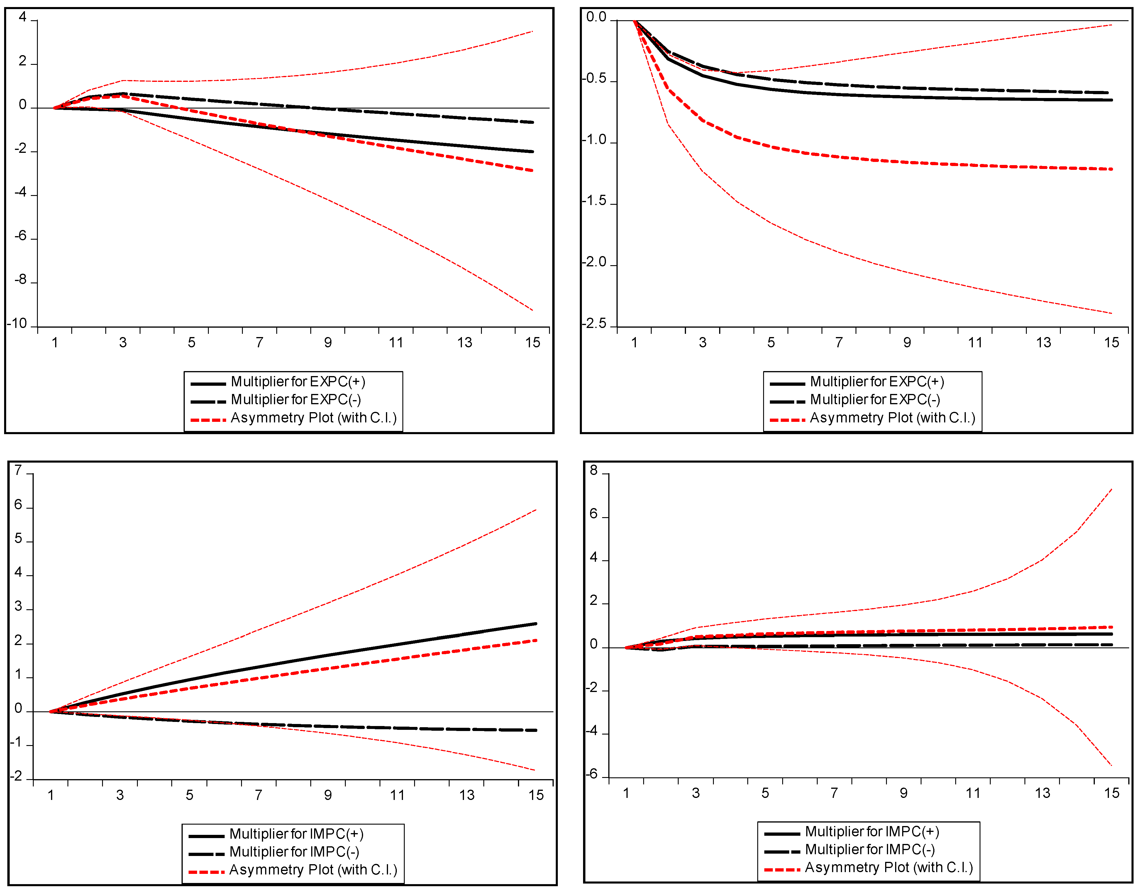
This study analyzes the symmetric and asymmetric effects of imports and exports on CBEs, utilizing data from two energy superpowers, the PRC and the USA, from 1990 to 2018. The ARDL and NARDL techniques are used to analyze the long-term and short-term correlations among the study variables. This study is the inaugural examination of the symmetric and asymmetric links between imports and exports for the two principal energy consumers globally, revealing, through the ARDL results, that exports diminish while imports augment CBEs in both the long and short term for the PRC and the USA. The long-term NARDL estimates indicate that an increase in exports diminishes CBEs, but increases in imports augment CBEs, for both economies. Meanwhile, the short-term estimates from NARDL indicate that an increase in imports boosts CBEs in both nations; however, a fall in exports enhances CBEs in the USA, while reducing CBEs in the PRC. This is attributed to the structural characteristics of the supply chain within each country.

Moreover, in the long run, the magnitude of the overall coefficients for the PRC surpasses that of the USA due to the overall pace of growth in trade and the reliance on energy-intensive imports in the PRC. The error correction term indicates that, following a shock in the short run, the PRC takes 2.6 times longer to return to an equilibrium state in the long run compared to the USA, reflecting the systemic rigidity of the PRC’s emissions and industrial systems. The data do not substantiate the Environmental Kuznets Curve (EKC) theory, which posits an inverted U-shaped correlation between economic expansion and emissions. This deviation from the EKC hypothesis might be ascribed to the neglect of emissions embedded in international commerce when evaluating the growth–emissions correlation. The dependence on consumption-based emissions underscores the necessity of a more holistic carbon accounting method, especially for economies with substantial trade volumes. Robustness checks, including dynamic ordinary least squares (DOLS) analysis and Granger causality tests, validate the consistency of these findings.

This study proposes the following subsequent policy implications derived from its findings. This study shows that higher economic growth intensifies CBEs, emphasizing the importance of decoupling economic growth from carbon emissions through structural reforms and low-carbon technologies. We recommend that both the PRC and the USA use energy-efficient technologies and augment the proportion of renewable energy in their overall energy portfolio to diminish their products’ energy intensity and emission levels. Imposing a carbon price on energy-intensive products will enable consumers to transition to less energy-intensive alternatives while incentivizing firms to decrease their energy intensity to remain competitive globally. Trade policies must concurrently account for the carbon footprints of traded items, necessitating strategies to assist domestic enterprises in diminishing the carbon footprints of their offerings. Transitioning from production-based to consumption-based accounting in international agreements can distribute emissions responsibility more equally. This would urge importing countries to consider the emissions inherent in their consumption habits, promoting shared responsibility.

In a manner analogous to tags that display energy consumption on electronic devices, energy-intensity labels ought to be affixed to all products, enabling consumers to factor in the energy intensity of the product in their decision-making processes. Furthermore, collaborative trade agreements should incorporate carbon standards, fostering mutual accountability and collective innovation in low-carbon technologies. Moreover, customized policies for high-emission industries, including heavy industry and transportation, like encouraging electrification in transportation and enhancing energy efficiency in manufacturing, can substantially decrease emissions associated with commerce. Lastly, the dependence on economic growth as a catalyst for carbon reductions, as suggested by the EKC, may prove inadequate. Both nations require creative policy instruments, like carbon border adjustments, green subsidies and more stringent emissions limits, to attain substantial reductions without depending exclusively on growth.

These policy actions highlight the importance of a comprehensive approach to managing trade-related emissions and ensuring sustainable growth for the PRC and the USA. This study’s methodological framework serves as a crucial resource for policymakers aiming to evaluate the long-term and short-term impacts of economic activity on carbon emissions. Future studies ought to broaden this analysis to include additional significant trading nations and examine sector-specific impacts to improve global carbon mitigation strategies.

References

1. NASA. Global Climate Change; NASA: Washington, DC, USA, 2024. Available online: https://climate.nasa.gov/ (accessed on 12 March 2025).
2. UNFCCC. The Paris Agreement; United Nations Framework Convention on Climate Change; UN: New York, NY, USA, 2016. [Google Scholar]
3. Shigeto, S.; Yamagata, Y.; Ii, R.; Hidaka, M.; Horio, M. An easily traceable scenario for 80% CO2 emission reduction in Japan through the final consumption-based CO2 emission approach: A case study of Kyoto-city. Appl. Energy 2012, 90, 201–205. [Google Scholar] [CrossRef]
4. Zhang, B.; Qiao, H.; Chen, Z.M.; Chen, B. Growth in embodied energy transfers via China’s domestic trade: Evidence from multi-regional input–output analysis. Appl. Energy 2016, 184, 1093–1105. [Google Scholar] [CrossRef]
5. Wiedmann, T. A review of recent multi-region input–output models used for consumption-based emission and resource accounting. Ecol. Econ. 2009, 69, 211–222. [Google Scholar] [CrossRef]
6. European Comission. Carbon Leakage; European Commission: Brussels, Belgium, 2020. [Google Scholar]
7. Weber, C.L. Uncertainties in constructing environmental multiregional input-output models. In Proceedings of the International Input-Output Meeting on Managing the Environment, Seville, Spain, 9–11July 2008; pp. 1–31. [Google Scholar]
8. Böhringer, C.; Schneider, J.; Asane-Otoo, E. Trade in carbon and carbon tariffs. Environ. Resour. Econ. 2021, 78, 669–708. [Google Scholar] [CrossRef]
9. Peters, G.P. From production-based to consumption-based national emission inventories. Ecol. Econ. 2008, 65, 13–23. [Google Scholar] [CrossRef]
10. Munksgaard, J.; Pedersen, K.A. CO2 accounts for open economies: Producer or consumer responsibility? Energy Policy 2001, 29, 327–334. [Google Scholar] [CrossRef]
11. Mi, Z.; Zheng, J.; Meng, J.; Zheng, H.; Li, X.; Coffman, D.M.; Woltjer, J.; Wang, S.; Guan, D. Carbon emissions of cities from a consumption-based perspective. Appl. Energy 2019, 235, 509–518. [Google Scholar] [CrossRef]
12. Karakaya, E.; Yılmaz, B.; Alataş, S. How production-based and consumption-based emissions accounting systems change climate policy analysis: The case of CO2 convergence. Environ. Sci. Pollut. Res. 2019, 26, 16682–16694. [Google Scholar] [CrossRef]
13. Kaushal, K.R.; Rosendahl, K.E. Taxing consumption to mitigate carbon leakage. Environ. Resour. Econ. 2020, 75, 151–181. [Google Scholar] [CrossRef]
14. Akalpler, E.; Hove, S. Carbon emissions, energy use, real GDP per capita and trade matrix in the Indian economy-an ARDL approach. Energy 2019, 168, 1081–1093. [Google Scholar] [CrossRef]
15. Haug, A.A.; Ucal, M. The role of trade and FDI for CO2 emissions in Turkey: Nonlinear relationships. Energy Econ. 2019, 81, 297–307. [Google Scholar] [CrossRef]
16. Shahbaz, M.; Nasreen, S.; Ahmed, K.; Hammoudeh, S. Trade openness–carbon emissions nexus: The importance of turning points of trade openness for country panels. Energy Econ. 2017, 61, 221–232. [Google Scholar] [CrossRef]
17. Afesorgbor, S.K.; Demena, B.A. Trade openness and environmental emissions: Evidence from a meta-analysis. Environ. Resour. Econ. 2022, 81, 287–321. [Google Scholar] [CrossRef]
18. Zhang, Y.; Zhang, S. The impacts of GDP, trade structure, exchange rate and FDI inflows on China’s carbon emissions. Energy Policy 2018, 120, 347–353. [Google Scholar] [CrossRef]
19. Yang, L.; Wang, J.; Shi, J. Can China meet its 2020 economic growth and carbon emissions reduction targets? J. Clean. Prod. 2017, 142, 993–1001. [Google Scholar] [CrossRef]
20. Özokcu, S.; Özdemir, Ö. Economic growth, energy, and environmental Kuznets curve. Renew. Sustain. Energy Rev. 2017, 72, 639–647. [Google Scholar] [CrossRef]
21. Ozcan, B.; Tzeremes, N.G.; Tzeremes, P.G. Energy consumption, economic growth and environmental degradation in OECD countries. Econ. Model. 2020, 84, 203–213. [Google Scholar] [CrossRef]
22. Bernard, J.-T.; Gavin, M.; Khalaf, L.; Voia, M. Environmental Kuznets curve: Tipping points, uncertainty and weak identification. Environ. Resour. Econ. 2015, 60, 285–315. [Google Scholar] [CrossRef]
23. Khan, Z.; Ali, M.; Liu, Y.; Shahbaz, M.; Yang, S. Consumption-based carbon emissions and trade nexus: Evidence from nine oil exporting countries. Energy Econ. 2020, 89, 104806. [Google Scholar] [CrossRef]
24. Hasanov, F.J.; Liddle, B.; Mikayilov, J.I. The impact of international trade on CO2 emissions in oil exporting countries: Territory vs consumption emissions accounting. Energy Econ. 2018, 74, 343–350. [Google Scholar] [CrossRef]
25. Liddle, B. Consumption-based accounting and the trade-carbon emissions nexus. Energy Econ. 2018, 69, 71–78. [Google Scholar] [CrossRef]
26. Knight, K.W.; Schor, J.B. Economic growth and climate change: A cross-national analysis of territorial and consumption-based carbon emissions in high-income countries. Sustainability 2014, 6, 3722–3731. [Google Scholar] [CrossRef]
27. UN-WTO. UN World Tourism Organization-Statistics; UN-WTO: Madrid, Spain, 2024. [Google Scholar]
28. IEA. Data and Statistics; IEA: Paris, France, 2024. [Google Scholar]
29. Popp, D. Induced innovation and energy prices. Am. Econ. Rev. 2002, 92, 160–180. [Google Scholar] [CrossRef]
30. Shahbaz, M.; Nasir, M.A.; Roubaud, D. Environmental degradation in France: The effects of FDI, financial development, and energy innovations. Energy Econ. 2018, 74, 843–857. [Google Scholar] [CrossRef]
31. Wiebe, K.S.; Gandy, S.; Lutz, C. Policies and consumption-based carbon emissions from a top-down and a bottom-up perspective. Low Carbon Econ. 2016, 7, 21–35. [Google Scholar] [CrossRef]
32. Redding, S.; Amiti, M.; Weinstein, D. The impact of the 2018 trade war on US prices and welfare (CEP Discussion Papers 1603); London School of Economics and Political Science, Centre for Economic Performance: London, UK, 2019. [Google Scholar]
33. Bown, C.P. The US–China trade war and phase one agreement. J. Policy Model. 2021, 43, 805–843. [Google Scholar] [CrossRef]
34. Hanif, I. Impact of economic growth, nonrenewable and renewable energy consumption, and urbanization on carbon emissions in Sub-Saharan Africa. Environ. Sci. Pollut. Res. 2018, 25, 15057–15067. [Google Scholar] [CrossRef]
35. Carfora, A.; Pansini, R.V.; Scandurra, G. The causal relationship between energy consumption, energy prices and economic growth in Asian developing countries: A replication. Energy Strategy Rev. 2019, 23, 81–85. [Google Scholar] [CrossRef]
36. Salman, M.; Long, X.; Dauda, L.; Mensah, C.N. The impact of institutional quality on economic growth and carbon emissions: Evidence from Indonesia, South Korea and Thailand. J. Clean. Prod. 2019, 241, 118331. [Google Scholar] [CrossRef]
37. Kim, D.-H.; Suen, Y.-B.; Lin, S.-C. Carbon dioxide emissions and trade: Evidence from disaggregate trade data. Energy Econ. 2019, 78, 13–28. [Google Scholar] [CrossRef]
38. Al-Mulali, U.; Ozturk, I.; Solarin, S.A. Investigating the environmental Kuznets curve hypothesis in seven regions: The role of renewable energy. Ecol. Indic. 2016, 67, 267–282. [Google Scholar] [CrossRef]
39. Gozgor, G. Does trade matter for carbon emissions in OECD countries? Evidence from a new trade openness measure. Environ. Sci. Pollut. Res. Int. 2017, 24, 27813–27821. [Google Scholar] [CrossRef] [PubMed]
40. Sharif Hossain, M. Panel estimation for CO2 emissions, energy consumption, economic growth, trade openness and urbanization of newly industrialized countries. Energy Policy 2011, 39, 6991–6999. [Google Scholar] [CrossRef]
41. Ang, B.W.; Su, B. Carbon emission intensity in electricity production: A global analysis. Energy Policy 2016, 94, 56–63. [Google Scholar] [CrossRef]
42. Shahbaz, M.; Lean, H.H.; Shabbir, M.S. Environmental Kuznets curve hypothesis in Pakistan: Cointegration and Granger causality. Renew. Sustain. Energy Rev. 2012, 16, 2947–2953. [Google Scholar] [CrossRef]
43. Marzouk, O.A. Summary of the 2023 report of TCEP (tracking clean energy progress) by the international energy agency (IEA), and proposed process for computing a single aggregate rating. E3S Web Conf. 2025, 601, 00048. [Google Scholar] [CrossRef]
44. Lin, B.; Ahmad, I. Analysis of energy related carbon dioxide emission and reduction potential in Pakistan. J. Clean. Prod. 2017, 143, 278–287. [Google Scholar] [CrossRef]
45. Grossman, G.M.; Krueger, A.B. Economic growth and the environment. Q. J. Econ. 1995, 110, 353–377. [Google Scholar] [CrossRef]
46. Ali, W.; Abdullah, A.; Azam, M. Re-visiting the environmental Kuznets curve hypothesis for Malaysia: Fresh evidence from ARDL bounds testing approach. Renew. Sustain. Energy Rev. 2017, 77, 990–1000. [Google Scholar] [CrossRef]
47. Apergis, N. Environmental Kuznets curves: New evidence on both panel and country-level CO2 emissions. Energy Econ. 2016, 54, 263–271. [Google Scholar] [CrossRef]
48. Dinda, S. Environmental Kuznets curve hypothesis: A survey. Ecol. Econ. 2004, 49, 431–455. [Google Scholar] [CrossRef]
49. Apergis, N.; Payne, J.E. Renewable energy consumption and economic growth: Evidence from a panel of OECD countries. Energy Policy 2010, 38, 656–660. [Google Scholar] [CrossRef]
50. Töbelmann, D.; Wendler, T. The impact of environmental innovation on carbon dioxide emissions. J. Clean. Prod. 2020, 244, 118787. [Google Scholar] [CrossRef]
51. Mohamued, E.A.; Ahmed, M.; Pypłacz, P.; Liczmańska-Kopcewicz, K.; Khan, M.A. Global oil price and innovation for sustainability: The impact of R&D spending, oil price and oil price volatility on GHG emissions. Energies 2021, 14, 1757. [Google Scholar] [CrossRef]
52. Gillingham, K.; Rapson, D.; Wagner, G. The rebound effect and energy efficiency policy. Rev. Environ. Econ. Policy 2016. Available online: https://www.jstor.org/stable/resrep01115 (accessed on 12 March 2025).
53. Dauda, L.; Long, X.; Mensah, C.N.; Salman, M.; Boamah, K.B.; Ampon-Wireko, S.; Kofi Dogbe, C.S. Innovation, trade openness and CO2 emissions in selected countries in Africa. J. Clean. Prod. 2021, 281, 125143. [Google Scholar] [CrossRef]
54. Friedlingstein, P.; Jones, M.W.; O’sullivan, M.; Andrew, R.M.; Hauck, J.; Peters, G.P.; Peters, W.; Pongratz, J.; Sitch, S.; Le Quéré, C. Global carbon budget 2019. Earth Syst. Sci. Data 2019, 11, 1783–1838. [Google Scholar] [CrossRef]
55. Acemoglu, D.; Aghion, P.; Bursztyn, L.; Hemous, D. The environment and directed technical change. Am. Econ. Rev. 2012, 102, 131–166. [Google Scholar] [CrossRef]
56. Shahbaz, M.; Hye, Q.M.A.; Tiwari, A.K.; Leitão, N.C. Economic growth, energy consumption, financial development, international trade and CO2 emissions in Indonesia. Renew. Sustain. Energy Rev. 2013, 25, 109–121. [Google Scholar] [CrossRef]
57. Sadorsky, P. The impact of financial development on energy consumption in emerging economies. Energy Policy 2010, 38, 2528–2535. [Google Scholar] [CrossRef]
58. Zhang, Y.-J. The impact of financial development on carbon emissions: An empirical analysis in China. Energy Policy 2011, 39, 2197–2203. [Google Scholar] [CrossRef]
59. Tamazian, A.; Rao, B.B. Do economic, financial and institutional developments matter for environmental degradation? Evidence from transitional economies. Energy Econ. 2010, 32, 137–145. [Google Scholar] [CrossRef]
60. Javid, M.; Sharif, F. Environmental Kuznets curve and financial development in Pakistan. Renew. Sustain. Energy Rev. 2016, 54, 406–414. [Google Scholar] [CrossRef]
61. Kahuthu, A. Economic growth and environmental degradation in a global context. Environ. Dev. Sustain. 2006, 8, 55–68. [Google Scholar] [CrossRef]
62. Managi, S.; Hibiki, A.; Tsurumi, T. Does trade openness improve environmental quality? J. Environ. Econ. Manag. 2009, 58, 346–363. [Google Scholar] [CrossRef]
63. Malik, M.Y.; Latif, K.; Khan, Z.; Butt, H.D.; Hussain, M.; Nadeem, M.A. Symmetric and asymmetric impact of oil price, FDI and economic growth on carbon emission in Pakistan: Evidence from ARDL and non-linear ARDL approach. Sci. Total Environ. 2020, 726, 138421. [Google Scholar] [CrossRef]
64. Al-mulali, U.; Sheau-Ting, L. Econometric analysis of trade, exports, imports, energy consumption and CO2 emission in six regions. Renew. Sustain. Energy Rev. 2014, 33, 484–498. [Google Scholar] [CrossRef]
65. Lamb, W.F.; Steinberger, J.K.; Bows-Larkin, A.; Peters, G.P.; Roberts, J.T.; Wood, F.R. Transitions in pathways of human development and carbon emissions. Environ. Res. Lett. 2014, 9, 014011. [Google Scholar] [CrossRef]
66. Androniceanu, A.; Georgescu, I. The impact of CO2 emissions and energy consumption on economic growth: A panel data analysis. Energies 2023, 16, 1342. [Google Scholar] [CrossRef]
67. Safi, A.; Chen, Y.; Wahab, S.; Ali, S.; Yi, X.; Imran, M. Financial instability and consumption-based carbon emission in E-7 countries: The role of trade and economic growth. Sustain. Prod. Consum. 2021, 27, 383–391. [Google Scholar] [CrossRef]
68. Kirikkaleli, D.; Güngör, H.; Adebayo, T.S. Consumption-based carbon emissions, renewable energy consumption, financial development and economic growth in Chile. Bus. Strategy Environ. 2022, 31, 1123–1137. [Google Scholar] [CrossRef]
69. Abbasi, K.R.; Hussain, K.; Haddad, A.M.; Salman, A.; Ozturk, I. The role of financial development and technological innovation towards sustainable development in Pakistan: Fresh insights from consumption and territory-based emissions. Technol. Forecast. Soc. 2022, 176, 121444. [Google Scholar] [CrossRef]
70. Qin, L.; Malik, M.Y.; Latif, K.; Khan, Z.; Siddiqui, A.W.; Ali, S. The salience of carbon leakage for climate action planning: Evidence from the next eleven countries. Sustain. Prod. Consum. 2021, 27, 1064–1076. [Google Scholar] [CrossRef]
71. Wiebe, K.S.; Yamano, N. Estimating CO2 Emissions Embodied in Final Demand and Trade Using the OECD ICIO 2015. 2016. Available online: https://www.oecd.org/en/publications/estimating-co2-emissions-embodied-in-final-demand-and-trade-using-the-oecd-icio-2015_5jlrcm216xkl-en.html (accessed on 12 March 2025).
72. Steinberger, J.K.; Timmons Roberts, J.; Peters, G.P.; Baiocchi, G. Pathways of human development and carbon emissions embodied in trade. Nat. Clim. Chang. 2012, 2, 81–85. [Google Scholar] [CrossRef]
73. Peters, G.P.; Hertwich, E.G. Post-Kyoto greenhouse gas inventories: Production versus consumption. Clim. Chang. 2008, 86, 51–66. [Google Scholar] [CrossRef]
74. Zhang, S.; Wei, J.; Chen, X.; Zhao, Y. China in global wind power development: Role, status and impact. Renew. Sustain. Energy Rev. 2020, 127, 109881. [Google Scholar] [CrossRef]
75. Sovacool, B.K.; Schmid, P.; Stirling, A.; Walter, G.; MacKerron, G. Differences in carbon emissions reduction between countries pursuing renewable electricity versus nuclear power. Nat. Energy 2020, 5, 928–935. [Google Scholar] [CrossRef]
76. Itkonen, J.V.A. Problems estimating the carbon Kuznets curve. Energy 2012, 39, 274–280. [Google Scholar] [CrossRef]
77. Jaforullah, M.; King, A. The econometric consequences of an energy consumption variable in a model of CO2 emissions. Energy Econ. 2017, 63, 84–91. [Google Scholar] [CrossRef]
78. Kilian, L. Not all oil price shocks are alike: Disentangling demand and supply shocks in the crude oil market. Am. Econ. Rev. 2009, 99, 1053–1069. [Google Scholar] [CrossRef]
79. Hamilton, J.D. What is an oil shock? J. Econom. 2003, 113, 363–398. [Google Scholar] [CrossRef]
80. Barsky, R.B.; Kilian, L. Oil and the Macroeconomy Since the 1970s. J. Econ. Perspect. 2004, 18, 115–134. [Google Scholar] [CrossRef]
81. Backus, D.K.; Crucini, M.J. Oil prices and the terms of trade. J. Int. Econ. 2000, 50, 185–213. [Google Scholar] [CrossRef]
82. Kallis, G.; Sager, J. Oil and the economy: A systematic review of the literature for ecological economists. Ecol. Econ. 2017, 131, 561–571. [Google Scholar] [CrossRef]
83. Jones, G.A.; Warner, K.J. The 21st century population-energy-climate nexus. Energy Policy 2016, 93, 206–212. [Google Scholar] [CrossRef]
84. Nasir, M.A.; Naidoo, L.; Shahbaz, M.; Amoo, N. Implications of oil prices shocks for the major emerging economies: A comparative analysis of BRICS. Energy Econ. 2018, 76, 76–88. [Google Scholar] [CrossRef]
85. Ju, K.; Su, B.; Zhou, D.; Wu, J. Does energy-price regulation benefit China’s economy and environment? Evidence from energy-price distortions. Energy Policy 2017, 105, 108–119. [Google Scholar] [CrossRef]
86. Troster, V.; Shahbaz, M.; Uddin, G.S. Renewable energy, oil prices, and economic activity: A Granger-causality in quantiles analysis. Energy Econ. 2018, 70, 440–452. [Google Scholar] [CrossRef]
87. Zaidi, S.A.H.; Zafar, M.W.; Shahbaz, M.; Hou, F. Dynamic linkages between globalization, financial development and carbon emissions: Evidence from Asia Pacific Economic Cooperation countries. J. Clean. Prod. 2019, 228, 533–543. [Google Scholar] [CrossRef]
88. Xu, B.; Lin, B. Does the high-tech industry consistently reduce CO2 emissions? Results from nonparametric additive regression model. Environ. Impact Assess. 2017, 63, 44. [Google Scholar] [CrossRef]
89. Pablo-Romero, M.d.P.; Sánchez-Braza, A. Productive energy use and economic growth: Energy, physical and human capital relationships. Energy Econ. 2015, 49, 420–429. [Google Scholar] [CrossRef]
90. Vancauteren, M. The effects of human capital, R&D and firm’s innovation on patents: A panel study on Dutch food firms. J. Technol. Transf. 2018, 43, 901–922. [Google Scholar] [CrossRef]
91. Lu, J.; Mao, X.; Wang, M.; Liu, Z.; Song, P. Global and national environmental impacts of the US–China Trade War. Environ. Sci. Technol. 2020, 54, 16108–16118. [Google Scholar] [CrossRef]
92. Amiti, M.; Redding, S.J.; Weinstein, D.E. The impact of the 2018 tariffs on prices and welfare. J. Econ. Perspect. 2019, 33, 187–210. [Google Scholar] [CrossRef]
93. Pesaran, M.H.; Shin, Y.; Smith, R.J. Bounds testing approaches to the analysis of level relationships. J. Appl. Econom. 2001, 16, 289–326. [Google Scholar] [CrossRef]
94. Andrews, D.W. Tests for parameter instability and structural change with unknown change point. Econom. J. Econom. Soc. 1993, 61, 821–856. [Google Scholar] [CrossRef]
95. Lee, J.; Strazicich, M.C. Minimum lagrange multiplier unit root test with two structural breaks. Rev. Econ. Stat. 2003, 85, 1082–1089. [Google Scholar] [CrossRef]
96. Hargreaves, S. Gas prices hit highest average ever in 2012. CNN, 31 December 2012. Available online: https://money.cnn.com/2012/12/31/news/economy/gas-prices/index.html (accessed on 12 March 2025).
97. Pesaran, M.H.; Smith, R. Estimating long-run relationships from dynamic heterogeneous panels. J. Econ. 1995, 68, 79–113. [Google Scholar] [CrossRef]
98. Odhiambo, N.M. Energy consumption and economic growth nexus in Tanzania: An ARDL bounds testing approach. Energy Policy 2009, 37, 617–622. [Google Scholar] [CrossRef]
99. Shin, Y.; Yu, B.; Greenwood-Nimmo, M. Modelling asymmetric cointegration and dynamic multipliers in a nonlinear ARDL framework. In Festschrift in Honor of Peter Schmidt: Econometric Methods and Applications; Sickles, R.C., Horrace, W.C., Eds.; Springer: New York, NY, USA, 2014; pp. 281–314. [Google Scholar] [CrossRef]
100. World Trade Organization. WTO Stats; World Trade Organization: Geneva, Switzerland, 2024. [Google Scholar]
101. Wu, Y.; Xiong, Y.; Tian, X.; Liu, Y.; Shi, F. Decoding the carbonization mode of the south coastal economic zone in China from the perspective of a dynamic industrial structure. J. Clean. Prod. 2018, 199, 518–528. [Google Scholar] [CrossRef]
102. Tian, X.; Chang, M.; Lin, C.; Tanikawa, H. China’s carbon footprint: A regional perspective on the effect of transitions in consumption and production patterns. Appl. Energy 2014, 123, 19–28. [Google Scholar] [CrossRef]
103. UN Environment Programme. Emissions Gap Report 2019; United Nations: Geneva, Switzerland, 2019. [Google Scholar]
104. He, G.; Lin, J.; Zhang, Y.; Zhang, W.; Larangeira, G.; Zhang, C.; Peng, W.; Liu, M.; Yang, F. Enabling a rapid and just transition away from coal in china. One Earth 2020, 3, 187–194. [Google Scholar] [CrossRef] [PubMed]
105. IEA. USA Energy Mix; IEA: Paris, France, 2024. [Google Scholar]
106. Wang, F.; Sun, J.; Liu, Y.S. Institutional pressure, ultimate ownership, and corporate carbon reduction engagement: Evidence from China. J. Bus. Res. 2019, 104, 14–26. [Google Scholar] [CrossRef]
107. Jiang, Z.; Wang, Z.; Li, Z. The effect of mandatory environmental regulation on innovation performance: Evidence from China. J. Clean. Prod. 2018, 203, 482–491. [Google Scholar] [CrossRef]
108. Li, J.; Li, S. Energy investment, economic growth and carbon emissions in China—Empirical analysis based on spatial Durbin model. Energy Policy 2020, 140, 111425. [Google Scholar] [CrossRef]
109. Wu, D.; Zhang, Y.; Liu, B.; Wang, K.; Wang, Z.; Kang, J. Optimization of coal power phaseout pathways ensuring energy security: Evidence from Shandong, China’s largest coal power province. Energy Policy 2024, 192, 114180. [Google Scholar] [CrossRef]
110. United States Environmental Protection Agency. Fast Facts on Transportation Greenhouse Gas Emissions; United States Environmental Protection Agency: Washington, DC, USA, 2024. [Google Scholar]
111. Ballard, E.; Ramkumar, A. America’s ambitious climate plan is faltering. The Wall Street Journal, 23 September 2024. [Google Scholar]
112. Dong, B.; Wang, F.; Guo, Y. The global EKCs. Int. Rev. Econ. Financ. 2016, 43, 210–221. [Google Scholar] [CrossRef]
113. Krishnakumar, D.; Josukutty, C.A. China’s climate diplomacy and global environment challenges: The conflict between sustainable development and national interests. East Asia 2025, 42, 201–219. [Google Scholar] [CrossRef]
114. Saundry, P.D. Review of the United States energy system in transition. Energy Sustain. Soc. 2019, 9, 4. [Google Scholar] [CrossRef]
115. Revel, D. American Climate Prospectus: Economic Risks in the United States; Columbia University Press: New York, NY, USA, 2014. [Google Scholar]
116. Shahbaz, M.; Gozgor, G.; Adom, P.K.; Hammoudeh, S. The technical decomposition of carbon emissions and the concerns about FDI and trade openness effects in the United States. Int. Econ. 2019, 159, 56–73. [Google Scholar] [CrossRef]
117. Gao, H.; Li, J.; Liu, F.; Wu, J. State ownership and credit rationing: Evidence From China. Int. Rev. Econ. Financ. 2023, 88, 237–257. [Google Scholar] [CrossRef]
118. Cong, L.W.; Gao, H.; Ponticelli, J.; Yang, X. Credit allocation under economic stimulus: Evidence from China. Rev. Financ. Stud. 2019, 32, 3412–3460. [Google Scholar] [CrossRef]
119. UNCTAD. Trade and Development Report 2024; UNCTAD: Geneva, Switzerland, 2024. [Google Scholar]
120. Firth, M.; Lin, C.; Liu, P.; Wong, S.M. Inside the black box: Bank credit allocation in China’s private sector. J. Bank. Financ. 2009, 33, 1144–1155. [Google Scholar] [CrossRef]
121. Chen, Y.; Cheng, L.; Lee, C.-C.; Wang, C.-S. The impact of regional banks on environmental pollution: Evidence from China’s city commercial banks. Energy Econ. 2021, 102, 105492. [Google Scholar] [CrossRef]
122. Chandran Govindaraju, V.G.R.; Tang, C.F. The dynamic links between CO2 emissions, economic growth and coal consumption in China and India. Appl. Energy 2013, 104, 310–318. [Google Scholar] [CrossRef]
123. Li, Y.; Li, C. Fossil energy subsidies in China’s modern coal chemical industry. Energy Policy 2019, 135, 111015. [Google Scholar] [CrossRef]
124. Gillingham, K.; Stock, J.H. The cost of reducing greenhouse gas emissions. J. Econ. Perspect. 2018, 32, 53–72. [Google Scholar] [CrossRef]
125. Zhang, M.Y. How resilient is China’s ‘world’s factory’ to supply chain shifts? East Asia Forum, 18 May 2024. Available online: https://eastasiaforum.org/2024/05/18/how-resilient-is-chinas-worlds-factory-to-supply-chain-shifts/ (accessed on 12 March 2025).
126. International Trade Administration. Supply Chain News: White House Executive Order on America’s Supply Chains; International Trade Administration: Washington, DC, USA, 2021. [Google Scholar]
127. Lenzen, M. Consumption-based accounting of CO2 emissions. Econ. Syst. Res. 2016, 28, 314–326. [Google Scholar]
128. Peters, G.P.; Hertwich, E.G. CO2 embodied in international trade with implications for global climate policy. Environ. Sci. Technol. 2008, 42, 1401–1407. [Google Scholar] [CrossRef]
129. Kander, A.; Jiborn, M.; Moran, D.D.; Wiedmann, T.O. National greenhouse-gas accounting for effective climate policy on international trade. Nat. Clim. Chang. 2015, 5, 431–435. [Google Scholar] [CrossRef]
130. Andrew, R.; Peters, G.P.; Lennox, J. Approximation and regional aggregation in multi-regional input–output analysis for national carbon footprint accounting. Econ. Syst. Res. 2009, 21, 311–335. [Google Scholar] [CrossRef]
131. Kanemoto, K.; Lenzen, M.; Peters, G.P.; Moran, D.D.; Geschke, A. Frameworks for comparing emissions associated with production, consumption, and international trade. Environ. Sci. Technol. 2012, 46, 172–179. [Google Scholar] [CrossRef] [PubMed]
132. Wu, G.; Zeng, M.; Peng, L.; Liu, X.; Li, B.; Duan, J. China’s new energy development: Status, constraints and reforms. Renew. Sustain. Energy Rev. 2016, 53, 885–896. [Google Scholar] [CrossRef]
133. Kahrl, F.; Williams, J.; Jianhua, D.; Junfeng, H. Challenges to China’s transition to a low carbon electricity system. Energy Policy 2011, 39, 4032–4041. [Google Scholar] [CrossRef]
134. Engle, R.F.; Granger, C.W.J. Co-integration and error correction: Representation, estimation, and testing. Econometrica 1987, 55, 251–276. [Google Scholar] [CrossRef]
135. Adelowokan, O.A.; Babasanya, A.O.; Maku, O.E.; Adesoye, A.B. Unemployment, poverty and economic growth in Nigeria. J. Econ. Manag. 2019, 35, 5–17. [Google Scholar] [CrossRef]
136. Shahbaz, M.; Lean, H.H. The dynamics of electricity consumption and economic growth: A revisit study of their causality in Pakistan. Energy 2012, 39, 146–153. [Google Scholar] [CrossRef]
137. Gahlot, R. An analytical study on effect of FIIs & DIIs on Indian stock market. J. Transnatl. Manag. 2019, 24, 67–82. [Google Scholar] [CrossRef]
138. Alcantara, V.; Padilla, E. Input-output subsystems and pollution: An application to the service sector and CO2 emissions in Spain. Ecol. Econ. 2009, 68, 905–914. [Google Scholar] [CrossRef]
Figure 1. Sequence of methodology.
Energies 18 03238 g001
Figure 2. Lag selection criteria under VAR in the polynomial graph for the PRC (LHS) and the USA (RHS).
Energies 18 03238 g002