Abstract
This study investigates how various renewable energy technologies influence national carbon intensity (CO2 emissions per unit of GDP) across 184 countries over the period 2000–2020. In the context of Sustainable Development Goals (SDG 7 and SDG 13) and the post-Paris-Agreement policy landscape, it addresses the gap in understanding technology-specific decarbonization effects and the role of governance. A dynamic panel framework employing the Dynamic Common Correlated Effects (DCCE) estimator accounts for cross-sectional dependence and temporal persistence, while disaggregating total renewables into hydropower, wind, solar, and geothermal generation. Environmental regulation is incorporated as a moderating variable using the World Bank’s Regulatory Quality index. Empirical results demonstrate that higher renewable generation is associated with statistically significant reductions in carbon intensity, with hydropower showing the most consistent negative effect across all income groups. Solar and geothermal technologies yield substantial carbon-reducing impacts in lower-middle-income settings once supportive policies are in place. Wind exhibits heterogeneous outcomes: positive or insignificant effects in some high- and upper-middle-income panels prior to 2015, shifting toward neutral or negative after more stringent regulation. Interaction terms reveal that stronger regulatory environments amplify renewable-driven decarbonization, particularly for intermittent sources such as wind and solar. Key contributions include (1) a comprehensive global assessment of four disaggregated renewable technologies; (2) integration of regulatory quality into decarbonization pathways, illustrating post-2015 policy moderations; and (3) methodological advancement through a large-sample DCCE approach that captures unobserved common shocks and heterogeneous country dynamics. These findings inform targeted policy measures—such as prioritizing hydropower where feasible, strengthening regulatory frameworks, and tailoring technology strategies—to accelerate low-carbon energy transitions worldwide.
1. Introduction
In recent decades, mitigating carbon dioxide (CO2) emissions while sustaining economic growth has become a primary concern for both scholars and policymakers worldwide [1]. Early research on the energy–growth nexus (e.g., [2]) established that energy consumption and GDP are tightly interlinked; however, these studies often treated energy as a homogeneous aggregate. More recent work recognizes that the composition of energy—particularly the growth in renewable energy sources—plays a crucial role in shaping environmental outcomes [3,4]. For example, a study by [4] finds that in the Group of Seven (G7) countries, renewable energy consumption significantly reduces CO2 emissions, whereas fossil-fuel consumption exacerbates them. Similarly, a study by [3] demonstrates that countries with higher shares of renewables in total energy consumption exhibit stronger decoupling of emissions from economic growth.
Yet, heterogeneity across renewable technologies and institutional contexts complicates this general finding (Figure 1 provides an overview of global trends in renewable energy generation, illustrating the scale of renewable expansion over time). Ref. [5] conducts a panel analysis of 15 major renewable-energy-consuming economies and reveal that while some renewables (e.g., hydropower) consistently correlate with lower CO2, others (e.g., wind and solar) occasionally exhibit positive or insignificant associations with emissions—particularly in nations where grid integration challenges and regulatory frameworks remain underdeveloped. They argue that in upper-middle-income countries, rapid wind and solar deployment without adequate grid flexibility can result in increased reliance on fossil-fuel “peaking” plants during low-renewable periods, yielding a net uptick in CO2 [5]. This study builds on this insight by expanding the country sample to 184 nations (2000–2020) and disaggregating renewables into hydropower, wind, solar, and geothermal, thereby testing whether Saidi and Omri’s heterogeneity holds at a truly global level.
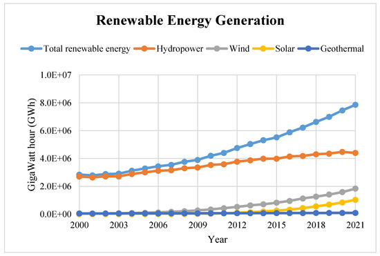
Figure 1.
Global trends in renewable energy generation.
Beyond cross-country comparisons, country-specific case studies underscore how infrastructure constraints and lifecycle emissions affect renewable–CO2 relationships. Ref. [6] conducts a life-cycle assessment of a multi-megawatt wind turbine and document that upstream emissions (manufacturing, transport, installation) are often externalized to regions still heavily dependent on coal-fired electricity. As such, a wind-rich country that imports turbine components may see only modest domestic CO2 reductions if the supply chain remains carbon-intensive. Ref. [7] further shows this, integrating large shares of wind capacity initially necessitated flexible gas-fired backup, which temporarily increased system-wide CO2 emissions during periods of low wind. These operational dynamics highlight that “environmental costs”—the unintended CO2 consequences of variability and supply-chain emission—can dampen or reverse expected decarbonization benefits in the short run [6,7].
On the policy front, a growing body of literature emphasizes the mediating role of governance and regulatory quality [8] in shaping renewable energy’s impact on environmental outcomes. Ref. [9] employs panel cointegration techniques across 30 provinces in China and find that better institutional quality accelerates the decarbonization effect of renewables. Similarly, ref. [10] shows that within the BRICS countries, the sign and magnitude of renewable–CO2 linkages hinge on the stringency of regulatory oversight, with weaker governance leading to “greenwashing” and underinvestment in grid upgrades. In this manuscript, we interact each disaggregated renewable source with the World Bank’s Regulatory Quality index, thereby providing one of the first large-sample tests of how institutional capacity transforms intermittent renewables from potential net-emitters into genuine decarbonization drivers—extending beyond the mainly cross-sectional or small-sample designs of prior studies [5,9,10,11,12].
Methodologically, much of the previous literature relies on static or two-step estimation techniques (e.g., fixed-effects, instrumental variables), which sometimes fail to capture the dynamic persistence and cross-sectional dependence inherent in CO2 emissions data. For instance, ref. [13] employs the Dynamic Common Correlated Effects (DCCE) estimator on a sample of newly industrialized countries and demonstrate that ignoring unobserved global shocks (such as oil-price spikes) biases estimates of renewable impacts. Likewise, ref. [14] shows that heterogeneous slope coefficients—reflecting different country-specific decarbonization pathways—must be accommodated to avoid misleading “one-size-fits-all” policy recommendations. By employing DCCE on 184 countries, this study is, to the best of our knowledge, the first to combine (a) comprehensive renewable disaggregation, (b) governance interactions, and (c) a large dynamic panel spanning low-income to high-income economies. This methodological innovation allows us to identify not only cross-country heterogeneity but also how the temporal evolution of policy (pre- vs. post-2015) alters renewable–CO2 relationships—a nuance seldom explored in existing work [13,14,15].
Finally, from a climate-policy perspective, this paper extends the debate on “green paradox” effects and short-run borrowing of cheaper coal [16]. While most studies emphasize mid- to long-run decarbonization benefits of renewables, ref. [17] argues that in the immediate term, subsidies and tax credits for wind and solar can temporarily depress fossil-fuel prices, delaying retirement of coal-fired plants. These paradoxical outcomes have been documented in fragmented national contexts (e.g., the U.S. Midwest), but few studies have tested their global prevalence. By splitting the sample into pre- and post-2015 periods and interacting renewable types with evolving regulatory metrics, we provide empirical evidence on whether post-Paris-Agreement regulatory tightening has successfully quelled these “green paradox” dynamics—something existing literature [5,16,17] has yet to address at scale.
In summary, the literature highlights that the environmental benefits of renewables depend on not just the scale of deployment but also on the broader institutional framework—especially the capacity of governments to enforce effective policies and regulations [18,19,20,21]. Yet, research on how these regulatory factors moderate the impact of renewables on carbon intensity is still limited. In addition, although prior research has examined individual renewable–CO2 linkages (e.g., [3,4]) and smaller heterogeneous panels (e.g., [5,13]), there remains a gap in simultaneously analyzing (1) four disaggregated renewable technologies, (2) regulatory-quality interactions, (3) pre-/post-2015 policy shifts, and (4) global coverage from low-income to high-income countries. This study fills this gap by leveraging a large, dynamic panel and DCCE methodology to deliver new insights into how the decarbonization efficacy of renewables is conditioned by both technological type and institutional setting.
That is to say, this study makes several key contributions. First, it provides a comprehensive global analysis of the decarbonization potential of renewable energy. Second, by integrating the moderating effect of environmental regulation, it extends the decarbonization pathways theory to account for institutional influences. Finally, the findings inform policy interventions that can maximize the climate benefits of renewable energy deployment. The remainder of the paper is organized as follows. Section 2 details the methodology, data sources, and model specifications. Section 3 presents the empirical results along with robustness tests. Section 4 discusses the implications of the findings for global decarbonization strategies, and Section 5 concludes with policy recommendations and suggestions for future research.
2. Materials and Methods
2.1. Data
The population is all the countries of the world, as this study considers the global perspective. The data utilized in this analysis exhibit an annual periodicity, and were obtained from their respective sources in 2023 as outlined in Table 1, spanning 1990 to 2022. However, not all variables had data values up till 2022 and also the early years of 1990s, and this limits the final sample covering the period from 2000 to 2020. For example, carbon dioxide emissions data obtained from the 2023 world development indicators (WDI) at http://www.worldbank.org is available up to the year 2020, so this limits the length of the carbon intensity (CI) variable derived by the authors. A representative sample consisting of 184 countries is utilized. The sample selection, as mentioned above, was based on data availability.

Table 1.
Variable definitions and sources.
The dependent variable is carbon intensity (CI). Mathematically, the carbon intensity of GDP is calculated as:
This metric aids in evaluating the effectiveness of resource allocation and the ecological consequences of economic growth. A reduced carbon intensity of gross domestic product implies that a nation generates economic productivity while emitting less carbon dioxide. This might serve as an indication of growth that is environmentally sustainable.
On the other hand, the independent variable is renewable energy generation, which considers wind (WE), solar (SE), hydropower (HP), and geothermal (GE) energy sources. The control variables used are foreign direct investment (FDI), population growth (POP) and urbanization (URB).
World Bank Worldwide Governance Indicators include aggregate country-level data on governance dimensions such as regulatory quality, rule of law, and control of corruption, which are relevant to environmental policy enforcement annually from 1996 onward. In this study, we use the Regulatory Quality indicator from the WGI as a proxy for environmental regulation. It captures perceptions of the government’s ability to design and implement sound policies and regulations, including those related to environmental protection. Reported in standard normal units (range: approx. −2.5 to 2.5), with higher values indicating stronger regulatory quality. Environmental regulation (ER) moderates the relationship between renewable energy generation and carbon intensity.
2.2. Model Specification
Analyzing the distinct impacts of different renewable energy technologies such as wind, solar photovoltaics, hydropower, and geothermal on carbon intensity reduction is crucial. The technical potential, policy incentives, lifecycle greenhouse gas emissions, and feasible deployment rates vary substantially for each technology based on their unique attributes. A disaggregated examination of individual renewable generation technologies enables modeling of optimized technology portfolios, designing targeted policy incentives, conducting comprehensive lifecycle emission assessments, and developing location-specific decarbonization projections. Rather than treating renewable energy generically, granular and nuanced technology-specific impact analysis provides vital insights into the most effective pathways, policies, and strategies to maximize cost-effective decarbonization through renewable electricity generation. Isolating the distinctive characteristics and carbon intensity effects of wind, solar, hydroelectric and geothermal power can inform rigorous research and evidence-based policymaking for climate change mitigation. This leads to Equation (2).
Also, economic growth theories link foreign direct investment, population, urbanization, and energy demand changes as countries develop [22]. Controlling for foreign direct investment, population and urbanization allows focusing on decarbonization while accounting for this wider relationship, resulting in Equation (3). Controlling for these variables removes any confounding effects. In addition, many studies analyzing drivers of carbon emissions use foreign direct investment, population and urbanization as standard control variables in regression models and find they are statistically significant [8,11,12,18,19,20,21].
2.2.1. Theoretical Framework: Decarbonization Pathways Theory
Decarbonization pathways theory posits that energy system transitions unfold gradually, shaped by historical legacies, technological inertia, and path-dependent infrastructures [23]. Under this framework, shifts from fossil fuels to low-carbon technologies are not instantaneous: existing capital stock, regulatory environments, and behavioral norms create inertia that slows change. The theory therefore emphasizes (a) the importance of gradual scale-up of renewables, (b) feedback effects from past emissions trajectories, and (c) the role of institutions in overcoming lock-in (see Figure 2) [23].

Figure 2.
Technical framework.
2.2.2. Application of the Decarbonization Pathways Theory to the Empirical Analysis
We operationalize decarbonization pathways theory by including a one-year lag of carbon intensity, L.lnCI, in the dynamic panel model. This lag captures the persistence and inertia of carbon intensity, reflecting that reductions achieved via renewable deployment materialize over multi-year horizons rather than instantaneously [13,14]. Specifically, in Equations (2)–(7), the term L.lnCI allows the model to account for the legacy effects of previous emissions, embedding the core mechanism of decarbonization pathways theory into the estimation strategy.
That is to say, the inclusion of this lag-dependent variable is both theoretically and empirically justified. Carbon intensity is not expected to adjust instantaneously to changes in renewable energy penetration or other influencing factors. Instead, it exhibits persistence over time due to technological inertia, infrastructural rigidity, policy implementation delays, and behavioral adaptation processes. This aligns with the decarbonization pathways theory, which suggests that transitions in energy systems and emission trajectories develop gradually and are influenced by historical legacies or path dependence (see Figure 2).
Empirically, incorporating L.lnCI within a dynamic panel estimation framework such as the Dynamic Common Correlated Effects (DCCE) estimator is crucial. This approach helps address potential endogeneity and omitted variable biases while capturing both the temporal autocorrelation and the heterogeneous nature of carbon intensity across a panel of 184 countries observed annually from 2000 to 2020. The selection of an annual lag is appropriate given the yearly frequency of the data and the recognition that systemic adjustments in energy systems and emissions often occur over a multi-year horizon.
Traditional estimation approaches such as ordinary least squares (OLS) and the generalized method of moments (GMM) yield consistent results under stringent stationarity assumptions and impose homogeneity of slopes; however, these methods may be insufficient when dealing with a mixed integration order (I(0) and I(1)) and cross-sectional dependencies. Therefore, we employ the approach of heterogeneous panels proposed by Chudik and Pesaran [14]. The combined use of this estimator with the inclusion of the lagged term L.lnCI provides more reliable estimates by accounting for feedback effects among the variables [13].
where all the parameters retain their meaning as described above. The natural log of the variables is denoted by ln. The intercept is , are the coefficients, and is the error term. The cross section and time parameters are and .
2.2.3. Justification for the Dynamic Common Correlated Effects (DCCE) Estimator
The Dynamic Common Correlated Effects (DCCE) estimator is particularly well suited to the study because it simultaneously addresses several key challenges inherent in multi-country panel data on decarbonization. First, by augmenting each country’s regression with cross-sectional averages of both the dependent and independent variables, DCCE effectively absorbs common shocks and spillover effects—such as global oil price fluctuations or coordinated regulatory shifts—that would otherwise bias estimates if left unmodeled [14,24]. Second, unlike homogeneous estimators that impose identical slope coefficients across units, DCCE permits heterogeneous slopes, thereby acknowledging that countries follow distinct decarbonization pathways shaped by their unique technological, institutional, and infrastructural contexts [14]. Third, because the regressors encompass a mixture of stationary and unit-root processes (e.g., GDP growth versus CO2 emissions trajectories), DCCE’s consistency in the presence of mixed integration orders prevents spurious inference that might arise under conventional estimators ill-equipped for such data [14]. Finally, by incorporating lagged dependent variables alongside common correlated effects, the DCCE framework mitigates endogeneity concerns and potential omitted-variable bias, ensuring more reliable inference about the dynamic relationship between renewable deployment, regulatory quality, and carbon intensity [13,14].
This leads to Equation (4) below.
In Equation (4), the cross-sectional means of the response variable and predictors are represented by , , , , , , , and , respectively. The lagged term (L.lnCI) captures the inertia and the persistence in carbon intensity, while the inclusion of cross-sectional means and lags of the predictors helps control for unobserved common shocks [13]. The notation represents the lag number of the cross-sectional mean. The average group estimates are computed using the formula:
In Equation (5), , and this is obtained by estimating the least-squares of Equation (4). Additionally, the asymptotic variance of the average group estimator is estimated using a non-parametric equation as follows:
Panel time series data consist of aggregated time trends and can display common shocks that change over time. The characteristics mentioned earlier in panel data could hinder the establishment of causal links. Furthermore, the incorporation of real-world data pertaining to carbon dioxide emissions includes short-term cyclical elements. This situation gives rise to the data’s susceptibility to reverse causality and potential inaccuracies in predicting long-term effects [23,25]. In order to mitigate these concerns raised, this study incorporate year effects into the analysis. This allows us to capture any overall temporal patterns and fluctuations in the data that may be attributed to common external factors. This study also accounted panel effects by considering economy type, region, and income level. These were performed as part of robustness checks. Finally, environmental regulation (ER) moderates the relationship as:
2.2.4. Reproducibility Protocol
The reproducibility protocol begins with data acquisition and initial filtering. Annual CSV files for CO2 emissions, GDP per capita, population growth, urbanization rate, and foreign direct investment were downloaded from the World Bank’s World Development Indicators (WDI) at https://databank.worldbank.org/source/world-development-indicators (accessed on 16 March 2023), while generation data for hydropower, wind, solar, and geothermal sources were obtained from IRENA’s 2023 Renewable Energy Statistics, at https://www.irena.org/Data (accessed on 16 March 2023). Regulatory Quality indices were sourced from the Worldwide Governance Indicators (WGI) at https://databank.worldbank.org/source/worldwide-governance-indicators (accessed on 16 March 2023). In Microsoft Excel, each dataset was filtered to include only the 184 sample countries (subject to data availability) over the period 2000–2020 as specified in Table 1. Whenever the same indicator appeared in more than one source, the version with the fewest missing observations was retained to ensure completeness.
Next, all filtered country–year sheets were cross-validated to detect and resolve inconsistencies. Country names and year formats were harmonized, and any mismatched values were reconciled by prioritizing the dataset with more comprehensive coverage. Following this quality check, the individual sheets were merged into a single file in Excel, providing an integrated panel dataset ready for statistical analysis.
The merged dataset was then imported into R studio for transformation and exploratory visualization. Natural-log transformations were applied to stabilize variance and approximate normality across all continuous variables [26]. A one-year lag of the log-transformed carbon-intensity variable (L.lnCI) was generated to capture policy and infrastructural inertia consistent with the decarbonization pathways framework [27]. Simple time-series plots were produced in Excel, while spatial choropleth maps illustrating geographic patterns were created in R studio.
Finally, the prepared dataset was exported from R v4.4.2 and loaded into Stata v15 for econometric estimation. The panel structure was declared with “tsset country year”, and the Dynamic Common Correlated Effects (DCCE) model was then estimated with robust standard errors.
Robustness checks included splitting the sample into pre-2015 and post-2015 periods and re-estimating the model within income- and region-based subsamples using Stata’s “by” prefixes.
3. Results
3.1. Results and Analysis
3.1.1. Cross-Sectional Dependency Analysis
Selecting the appropriate panel unit root test is made based on the results obtained from the cross-sectional dependency test. (Cross-sectional dependence in panel data occurs when the observations (or entities) in the panel are not independent of each other. In other words, the error terms for different entities are correlated. This violates one of the key assumptions of classical panel data models, which assumes that observations for different entities are independent). The second-generation cross-sectional dependence test is appropriate. However, this study employed both the first- and second-generation tests to test for cross-sectional dependence in the series in this study. This was performed to check the consistency of the results. Table 2 presents the results of the cross-section dependency test. The tests show that unobserved common shocks in the error term are statistically significant, and therefore, the second-generation panel unit root tests are more appropriate in testing the stationary property of the series. That is, the presence of cross-sectional dependence in the data favors the use of second-generation panel stationarity tests. (There are several means to address cross-sectional dependence in panel data. One of such include the use of Panel Data Models with Cross-Sectional Dependence. Some advanced panel data models explicitly account for cross-sectional dependence. For instance, models like the Common Correlated Effects (CCE) model are designed to handle this issue. As mentioned earlier, the Dynamic Common Correlated Effects (DCCE) model is used in this study as it is designed to address cross-sectional dependence in panel data. This model is an extension of the Common Correlated Effects (CCE) model, which itself is a panel data model that allows for unobserved common factors to affect all entities in the panel). The results of these tests are shown in Table 3, where all the variables are stationary after first differencing.
Table 2.
Cross-sectional dependence test.
Table 3.
CADF unit root test.
3.1.2. Unit-Root Test
A precondition for cointegration is the stationarity of the series. Thus, the study investigated the series’ stationarity properties by employing the CADF tests. The Cross-sectional Augmented Dickey–Fuller (CADF) test is a panel unit root test that allows for cross-sectional dependence in panel data, and it is therefore employed in this study. The CADF test extends the traditional Augmented Dickey–Fuller (ADF) test to panel data by incorporating additional lagged values of the dependent variable from other entities in the panel. So, this allows it to account for cross-sectional dependence.
Results from these tests are presented in Table 3, indicating the order of integration (since the variables are integrated of order 0 and order 1, that is, I(0) and I(1), it necessitates the use of the DCCE model, as discussed earlier). The tests revealed that some of the series had unit root at level but were all stationary after first differencing (see Table 3).
3.1.3. Baseline Regression Results
The results in Table 4 provide evidence that increased renewable energy generation is associated with statistically significant reductions in carbon intensity across the model specifications.
Table 4.
The role of renewable energy generation on carbon intensity.
The lagged dependent variable coefficients are negative and highly significant, indicating carbon intensity exhibits persistence but some degree of convergence over time. The key renewable energy generation variable enters negatively and significantly at the 1% level in all models, aligning with the hypothesis that higher renewable generation predicts lower subsequent carbon intensity.
Importantly, the Pesaran CD test statistics are insignificant in all models, providing no evidence of cross-sectional dependence concerns that would invalidate inference. Additionally, the models achieve reasonably high R-squared values, explaining substantial variation in carbon intensity.
The research is grouped into five main panels. Panel A is high-income countries, Panel B is upper-middle-income countries, Panel C is lower-middle-income countries, Panel D is low-income countries, and Panel E combines all the countries for empirical analysis.
From Table 4, the findings demonstrate that hydropower (HP) recorded a negative slope relationship with carbon intensity in all the panels. The negative association was statistically significant at 1% in all the panels. The results imply that a percentage increase in hydropower will correspond to a decrease in carbon intensity by 0.093, 0.065, 0.056, 0.046, and 0.118 in panels A, B, C, D, and E, respectively. The mechanism of the negative link is as a result of low pollution produced by hydropower [28]. According to the technological innovation theory, the production of hydroelectric power has significantly improved in terms of capacity, productivity, effectiveness and efficiency which has led to a decrease in carbon intensity. Thus, through this theory, hydropower plants can now generate energy from water flow more efficiently because of its advancements in turbine design, control systems, and material science. These results are in line with the theory and suggest that countries should increase the use of hydropower to decrease the environmental impact and achieve a sustainable environment. Moreover, decarbonization theory emphasizes the significance of switching from high-carbon to low-carbon energy sources, which lowers carbon intensity. Therefore, the theory aligns with the findings and suggest to countries in high-income, low-income, upper-middle-income, and lower-middle-income brackets to increase the use of hydropower so as to reduce carbon intensity in the countries. The results are supported by the findings of [29,30]. Moreover, the results contradict with the findings of [31].
However, wind energy (WE) recorded a positive link in all the panels. The positive slope relationship was statistically significant at 1% in panel B, 5% in panel D, 10% in panel E and insignificant in panels A and C. The significance relationship shows that an increase in wide energy will correspond to an increase in carbon intensity by 0.172, 0.145, and 0.351 for upper-middle-income countries, lower-middle-income countries and combinations of all countries. The results suggest that countries within this range should develop further technologies for power use to decrease carbon intensity rather than concentrating on wind energy for power generation, which increases carbon intensity. Moreover, the insignificant association implies that wind energy does not significantly impact carbon intensity in higher-income countries and lower-income countries. The positive mechanism is as a result of the environmental cost of wind energy [32]. Moreover, the results are in line with the technological innovation theory and suggest that countries should develop new technologies for power use rather than wind energy, which increases carbon intensity. Moreover, in order to achieve the sustainability development goals by 2030, countries should corroborate and adopt new technology for power use to reduce the environmental impact of wind energy. This result is in line with the findings of [5,28]. However, it contradicts the findings of [33].
Solar energy (SE) recorded a conflicting result in the panels. A positive slope relationship was found in panels A, B and D with carbon intensity. However, a negative link was found in panels C and D with carbon intensity. The relationship in the panels was statistically significant at 1%. The positive link implies that an increase in solar energy in high-income countries, upper-middle-income countries, and lower-middle-income countries will increase carbon intensity by 0.256, 0.164, and 0.074, respectively. This suggests that countries within these regions should decrease the use of solar energy as a source of power generation so as to reduce their environmental impact and remain sustainable. Thus, as nations move towards renewable energy sources, the positive slope connection between solar energy and carbon intensity will turn negative. Moreover, the environmental Kuznets hypothesis contends that the positive link should ultimately turn negative if a country’s per capita income rises over a certain level. This is a result of the tendency of governments and communities to actively lower carbon intensity and prioritize environmental protection after they reach a certain degree of economic growth. The results also suggest that policymakers should develop strategies in the adoption of new technology to generate power rather the concentrating mainly on solar energy per the technological innovation theory. The findings are supported by the findings of [5,31] and also contradict the findings of [33].
Moreover, geothermal energy (GE) recorded a negative slope relationship in panels A, C, and E. The negative slope was statistically significant at 5% in panels C and E and insignificant in panel A. The results imply that an increase in geothermal energy will correspond to a decrease in carbon intensity in panel C and E countries by 0.051 and 0.073, respectively. However, the insignificant relationship implies that an increase in geothermal energy does not significant impact carbon intensity in panel A. Additionally, a positive slope relationship was found in panels B and D countries. The positive slope relationship was significant at 1% in panel B and insignificant in panel D countries. Thus, an increase in geothermal energy will increase carbon intensity in panel B countries but will not have any effect on panel D countries. The results suggest that, since geothermal energy recorded a negative link in panel A, C and D countries, policymakers should adopt this energy use to decrease carbon intensity in the world so as to promote sustainability development goals of reducing pollution by 2030. The results correspond with the findings of [5,30,31] and contradict the findings of [34].
Regarding the control variables, population growth recorded a positive and statistically significant relationship with carbon intensity. The positive slope implies that an increase in population growth will result in an increase in carbon intensity in all the panel by 0.053, 0.034, 0.092, 0.038, and 0.098, respectively. The results suggest that as countries’ populations increase, adequate measures should be implemented to decrease carbon intensity so as to achieve the Sustainable Development Goals (SDGs). Moreover, urbanization rate recorded a negative slope link with carbon intensity in all the panels. This implies that an increase in urbanization rate will correspond to a decrease in carbon intensity. As a result, adequate measure should be embarked by law to reduce the impact of urbanization on carbon intensity. Lastly, FDI revealed a positive link in all the panels which is statistically significant at 1%. The positive link implies that an increase in FDI will correspond to an increase in carbon intensity by 0.084, 0.064, 0.054, 0.064 and 0.125, respectively.
The results reaffirm the results from the renewable energy trend analysis in Figure 2 and the correlation analysis where wind and solar energy demonstrate the strongest negative correlations with carbon intensity compared to hydropower and geothermal sources, suggesting the former two technologies may drive decarbonization effects more than the latter. However, uptake of wind and solar energy still remains at relatively low levels compared to hydropower (see Figure 3: solar and wind energy are less commonly adopted, as can be seen in the graph; however, they have a high carbon-intensity-reducing effect), despite their outsized emission reduction potential. The findings indicate there is still substantial potential to further reduce carbon intensity through expanding the adoption of solar and wind power. Significantly increasing the scale of solar photovoltaic and wind energy generation could provide sizable additional emissions reductions and low-carbon transition benefits going forward. The analysis shows that sizable decarbonization opportunities remain by accelerating the deployment of these renewable energy technologies.
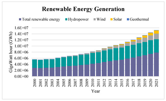
Figure 3.
Increasing trend of global renewable energy generation.
3.1.4. The Moderating Role of Environmental Regulation on Renewable Energy Generation and Carbon Intensity
This study employed environmental regulation as the moderator for the relationship between renewable energy generation and carbon intensity. Table 5 presents the results of the moderating role.
Table 5.
The moderating role of environmental regulation on REG and CI.
The regression model explains approximately 89.6%, 84.5%, 83.1%, 82.7%, and 72.1% of the variance in carbon intensity in Panel A, B, C, D and E, respectively. The high R-squared value indicates that the renewable energy sources in the model collectively account for a substantial proportion of the variation in all panels. It highlights that the model is effective in predicting changes in carbon intensity, and the independent variables have a strong explanatory power.
The CD statistics in all panels underscore that there is notable difference in the distribution of outcome before and after the treatment. The magnitude of the CD statistics indicates that the change in carbon intensity is relatively large and statistically significant.
The lagged carbon intensity (InCI) demonstrates a statistically significant negative influence on the current carbon the present carbon intensity in Panel A, B, C, D and E, underlining that the previous levels of carbon intensity have a reducing effect on the current carbon intensity. This implies that there is a form of negative autocorrelation where lower historical carbon intensity is associated with lower carbon intensity.
In Panel A, the connection between hydropower energy and environmental regulation shows a statistically significant negative effect on carbon intensity (CI). This underscores that an increase in the use of hydropower is related with carbon intensity. In Panel B, hydropower energy reveals a statistically significant adverse influence on carbon intensity. This highlights the potential of hydropower as a clean source of energy to reduce carbon intensity. In Panel C, hydropower demonstrates a statistically significant negative influence on carbon intensity, underscoring the capacity of hydropower as a renewable energy source to reduce carbon emissions. In Panel D, hydropower exhibits a statistically significant negative effect on carbon intensity, highlighting that increase in hydropower utilization is associated with a reduction in carbon intensity. In Panel E, there is a statistically significant adverse relationship between hydropower and carbon intensity, emphasizing the ability of hydropower to reduce carbon emissions.
Wind power and environmental regulation have a positive but statistically not significant relationship with carbon intensity (CI) in Panel A. This suggests that the impact of wind power on carbon intensity is weak. Panel B shows that wind power has a positive statistically significant connection with carbon intensity, highlighting that increased utilization of wind power correlates with higher carbon intensity. In Panel C, there is a positive and statistically insignificant association between wind power and carbon intensity, underlining that insufficient wind power energy does not influence high carbon intensity. In Panel D, wind power demonstrates a positive and statistically significant effect on carbon intensity, underscoring the benefit of the efficient utilization of wind power to reduce environmental impact. Panel E shows that wind power has a statistically significant positive association with carbon intensity. This implies that the utilization of wind power efficiently minimizes carbon emissions.
Solar energy and environmental regulation demonstrate a positive and statistically significant influence on carbon intensity in Panel A. This suggests that an increase in the use of solar energy leads to higher carbon intensity. In Panel B, solar energy shows a statistically positive influence on carbon intensity, underling the excessive utilization of solar energy leads to high carbon emission. Panel C demonstrates that solar energy has a negative and statistically significant effect on carbon intensity, underlining that increased utilization of solar energy results in lower carbon intensity. In Panel D, there is a positive and statistically significant relationship between solar energy and carbon intensity, emphasizing the need for planning when integrating solar energy to avoid increasing carbon emissions. Panel E exhibits that solar energy has a negative and statistically significant influence on carbon intensity, underlining the need for thoughtful integration of solar energy to minimize carbon emissions.
Geothermal energy has a negative but statistically insignificant relationship with carbon intensity in Panel A. This suggests that the effects of wind geothermal energy on reducing carbon intensity are weak. In Panel B, geothermal energy shows a positive statistically significant influence on carbon intensity. This underlines that geothermal energy contribute to higher carbon intensity levels. In Panel C, geothermal energy reveals a negative and statistically significant effect on carbon intensity. This underscores that geothermal energy leads to lower carbon intensity. In Panel D, geothermal energy has a positive but not statistically significant influence on carbon intensity. This result highlights the essence of efficiently utilizing geothermal energy to reduce carbon emissions in this panel. Panel D shows that geothermal energy has a statistically significant negative impact on carbon intensity. This suggests that geothermal energy leads to lower carbon intensity. These findings underscore the need for careful integration of geothermal energy to achieve desired carbon intensity reduction.
Finally, the results in Table 5 indicate that environmental regulation (ER) plays a moderating role in the relationship between renewable energy generation and carbon intensity. This moderating effect can be understood through several mechanisms. First, stringent environmental regulations often enhance the displacement of fossil fuels by both directly restricting high-emission activities and promoting the accelerated adoption of renewable energy projects. In this way, renewables replace carbon-intensive sources more effectively in regulated environments. Second, stronger regulatory frameworks create technological and operational incentives—such as subsidies, research and development support, and efficiency standards—that lead to more efficient renewable energy systems and grid operations. These improvements further reduce overall carbon emissions. Finally, clear policy targets and standards provided by robust ER send critical market signals, encouraging investment in renewables and facilitating the decommissioning of outdated, high-emission technologies.
Thus, the interaction terms in Table 5 (e.g., lnHP × ER and lnSE × ER) capture these direct and indirect influences, indicating that when ER is more stringent, the decarbonization impact of renewable energy is significantly amplified. This suggests that the effectiveness of renewable energy in reducing carbon intensity is not solely dependent on its scale of deployment but also strongly influenced by the broader regulatory environment in which the energy system operates.
3.2. Robustness Tests
3.2.1. Empirical Model Accounting for Aggregated Time Effects
There have been several global environmental and renewable energy policies over the years, especially between 2000 and 2020. One of these is The Paris Agreement, negotiated in 2015 at COP21, aiming to limit global warming well below 2 degrees Celsius above pre-industrial levels. The Paris Agreement officially entered into force in November 2016 and it seeks to enhance global efforts to combat climate change. Moreover, the adoption of the Sustainable Development Goals (SDGs) in 2015 introduced several global environmental and renewable energy policies to be achieved between the years 2015 and 2030. For the purpose of this study, we focus only on sustainable development goals 7, 9, and 13, representing affordable and clean energy for all, industry innovation and infrastructure, and climate action, respectively.
These global environmental and renewable energy policies above saw their implementation in 2015, making it imperative to study the contribution of the implementation of these policies on carbon intensity reduction. Hence, we included time effects. We then studied the impact of these global environmental and renewable energy policies on carbon intensity reduction before their implementation in 2015 and then after their implementation. Introducing time effects allowed us to see if the said policies significantly reduce carbon intensity. The introduction of time effects also helps check the robustness of the initial models.
Hence, to examine the robustness of the findings, we rerun the equation by employing a sample based on the selected years of the study thus before the implementation of the policies in 2015 and after the implementation of the policies.
We then sampled the years as before the implementation of the policies, from 2000 to 2015, and after the implementation of policies, from 2015 to 2020, to identify the significance level of the impact of the moderating role of environmental regulation on renewable energy generation and carbon intensity. Table 6 presents the robustness results for before the implementation of the policies, from 2000 to 2015, and Table 7 presents the robustness results for after the implementation of the policies, from 2015 to 2020.
Table 6.
Robustness test before the implementation of the policies.
Table 7.
Robustness test after the implementation of the policies.
The findings in both models demonstrate that the R-squared values recorded show significant variation in how the dependent variables affect the dependent variables. In addition, the Pesaran CD test statistics remain insignificant, providing no evidence of problematic cross-sectional dependence in the residuals that would invalidate inference. This further enhances the robustness of the findings.
The findings in Table 6 are for before the implementation of the policies, and Table 7 shows those after the implementation of the policies. The findings reveal that hydropower recorded a negative slope link both in Table 6 and Table 7, which was statistically significant at 1% level. By comparing the results, for after the implementation of the policies, a lower coefficient was recorded than before the implementation of the policies. This shows that the policies implemented by the Paris Agreements and the Sustainable Development Goals on global environmental and renewable energy have significantly decreased carbon intensity globally for high-income countries, upper-middle-income countries, lower-middle-income countries, and low-income countries. Thus, is it suggested that more effective policies on the impact of the environment should be implemented to achieve a sustainable growth worldwide. Furthermore, environmental regulations should be strengthened to enhance the quality of life of people.
Moreover, wind energy recorded a positive association of carbon intensity in both before the implementation of the policies and after the implementation of the policies. By comparing the results, it is shown that the coefficient of before the implementation of the policies is higher than after the implementation of the policies. Thus, the policies implemented have really decreased the positive impact of wind energy on carbon intensity globally. Moreover, effective environmental regulation initiated globally in countries has decreased the intensity of carbon emission. It is suggested that policymakers in nations should embrace the sustainability agenda by prioritizing the need for the effective implementation of eco-friendly policies to promote sustainable development.
Furthermore, solar energy recorded a conflicting result in Table 6 and Table 7. Thus, by comparing the results, Table 6 findings show a negative and statistically significant relationship between solar energy and carbon intensity. However, Table 7 results show a positive and statistically significant link at 1%. This implies that the implementation of the policies initiated by the Sustainable Development Goals and Paris Agreements on global environmental and renewable energy has significantly decreased carbon intensity globally through the reduction in the use of pollutant energy intensity instruments. As a result, policymakers are encouraged to strengthen environmental regulation policies supporting the Sustainability Development Goals and the Paris Agreement to promote environmental performance and decrease carbon intensity.
In addition, the robustness results of geothermal energy show that the implementation of the policies has significantly decreased the coefficient of carbon intensity in the countries. By comparing the results in Table 6 and Table 7, it can be seen that environmental regulations have improved the environmental performance of the countries after the implementation of the policies globally and have decreased carbon intensity. It is suggested that policymakers and stakeholders should strengthen policies, laws and regulations on the environment to reduce the negative impact of carbon intensity.
Finally, in high-income countries, the finding that increased wind generation is associated with a positive—and, in some cases, statistically insignificant—effect on carbon intensity likely reflects a confluence of factors beyond simple “environmental costs.” First, as wind capacity grows, high-income grids often encounter integration challenges: the need for flexible backup generation (frequently gas-fired plants) to balance variability can actually raise system-wide emissions, especially during periods of low wind and high demand [7]. Second, much of the lifecycle carbon embodied in modern turbines—including manufacture, transport, and installation—occurs in regions still reliant on coal power; high-income countries importing turbine components may thus externalize emissions, diluting the net decarbonization benefit domestically [6]. Third, as markets mature, additional wind capacity often delivers diminishing marginal returns: early projects replace high-emission baseload plants, but later additions primarily displace cleaner gas or even other renewables, yielding smaller—or, at times, slightly positive—marginal carbon intensities [15]. Finally, permitting delays and curtailment policies in densely populated, environmentally sensitive regions can reduce actual delivered output relative to installed capacity, further weakening the observed relationship [35]. Together, these operational, technological, and supply-chain dynamics help explain why, in high-income contexts, wind’s impact on carbon intensity may appear muted or—even counterintuitively—positive, and demonstrate that attributing it solely to “environmental costs” oversimplifies a complex system of trade-offs.
3.2.2. Robustness Test Controlling for Panel Effects Using Economy Type
As there have been some Clean Development Mechanisms (CDMs) over the study period, the Kyoto Protocol’s CDM, which entered into force in 2005, allowed industrialized countries to invest in emission-reduction projects in developing countries, and this includes renewable energy projects. As mentioned earlier, the Kyoto Protocol is an international treaty that aimed to reduce greenhouse gas emissions worldwide. It established legally binding emission reduction targets for developed countries. It mandated developed economies to invest in clean environmental and energy projects in emerging and developing economies. Hence, this research studied the panel effects among emerging economies and developed economies. This in itself is a robustness measure.
That is to say, as part of further robustness test, this study grouped the countries in two main categories: emerging economies and developed economies. Table 8 shows the results of the robustness of emerging and developing economies.
Table 8.
Empirical model using economy type to control for panel effects.
The results in Table 8 show R-squared values of 0.699 and 0.681 for emerging and developed economies, which shows the significant effect in the differences of how the independent variables affect the dependent variables. Moreover, the CD statistics remain insignificant, providing no evidence of problematic cross-sectional dependence in the residuals that would invalidate inference. This further enhances the robustness of the findings. The p-values also shows the high significance levels of the variables employed.
The models incorporating panel effects for emerging and developed economies in Table 8 provide additional robust evidence for the relationship between greater renewable energy generation and lower carbon intensity. The lagged dependent variable remains highly significant across all models, reaffirming the persistence of carbon intensity levels over time. This implies the decarbonization effect of increasing renewable generation holds regardless of economic development status. The magnitude of the effects is larger for developed nations, suggesting more pronounced impacts from renewables in these countries.
Regarding the independent variables, the findings show when disaggregating by technology, renewable sources like hydropower, wind and solar all exhibit larger effects in the developed economy samples compared to emerging nations. This shows that developed economies are more likely to exhibit high level of carbon intensity than developing economies. As a result, policymakers and stakeholders in both economies should strengthen environmental regulations, policies, and laws on renewable energy generation to decrease carbon intensity. Moreover, as environmental regulations have moderated the relationship which has significantly reduced carbon intensity, per the findings, policymakers should embrace the SDGs agenda on environmental innovation and growth to promote environmental performance in the long run. Furthermore, the technological innovation theory suggests that countries should adopt green innovation strategies to reduce the negative impact of industrial actions, including energy generation, production, construction, and other forms of industrial activities. Although emerging economies recorded lower coefficients than developed economies, policymakers in such countries should look to advance innovation methods for energy in general to reduce carbon intensity in the long term. In order to achieve the SDGs by 2030, advanced countries should collaborate with developing countries to promote technology and innovation so as to reduce carbon intensity in the long term.
In summary, the panel effect models reaffirm that the carbon intensity reduction impact of renewable expansion holds across both developed and emerging economies, despite differences in magnitude. This enhances confidence in the relationship as an important policy lever for decarbonization.
3.3. Spatial Analysis of Carbon Intensity, Pre- and Post-Intervention
The carbon intensity maps provide a visual perspective on how emissions per GDP have evolved spatially around the 2015 global policy intervention (see Figure 4).

Figure 4.
Spatial distribution of the sampled 184 countries’ carbon intensity: pre- and post-intervention period. (A) Prior to 2015 where intensity levels appear relatively high across most countries, with many nations concentrated in the upper end of the color scale, and with higher carbon intensity levels.; (B) 2015 data, where the spatial analysis provides indication that the global environmental and renewable energy policies implemented around 2015 may have accelerated an ongoing trend of declining carbon intensity internationally as per the 2015 data.; (C) After 2015, where noticeable overall declines in intensity is recorded, with most countries transitioning into the lower end of the color scale.
In the 2000 pre-intervention map in Figure 4A, intensity levels appear relatively high across most countries, with many nations concentrated in the upper end of the color scale. Of the 184 countries, Ukraine recorded the highest carbon intensity of 0.004258 in 2020. Uzbekistan ranks second, followed by Turkmenistan, Mongolia, Azerbaijan, Syrian Arab Republic, Belarus, Russian Federation, Serbia, Kazakhstan, Moldova, Bulgaria, and Iran, Islamic Rep., amongst others. In comparison, and with the exception of Iran and Russia, these countries’ carbon intensity in 2000 was higher than even that of the Organization of the Petroleum Exporting Countries (OPEC) and OPEC+ countries such as Iraq, Qatar, and Saudi Arabia, ranked 29th, 30th, and 43rd, respectively. This is likely due to the huge role of oil to the economic growth of these OPEC countries. Those countries with the highest carbon intensity are an indication of the relatively low economic impact in relation to the carbon they emit.
However, the 2020 map in Figure 4C shows noticeable overall declines in intensity, with most countries transitioning into the lower end of the color scale. Some regions like Uzbekistan, Belarus, and Azerbaijan declined more markedly than areas such as Syrian Arab Republic, Iran, Islamic Rep., Kyrgyz Republic, South Africa, and Bosnia and Herzegovina, which remained more carbon-intensive in terms of ranking.
The highest carbon intensity recorded declined from 0.004258 in 2000 to 0.00199 in 2015 through to 0.00167 in 2020. The spatial analysis provides indication that the global environmental and renewable energy policies implemented around 2015 may have accelerated an ongoing trend of declining carbon intensity internationally as per the 2015 data illustrated pictorially in Figure 4B. Connecting the maps to the econometric findings, the visualized intensity reductions coincide with the modeled relationship between increasing renewable generation and falling emissions intensity over this period. That is, the maps indicate a broad geographic pattern of carbon intensity reductions coinciding with the global climate policy timeline. The geographic overview complements the statistical model results. While not definitive evidence alone, the visualized downward shift and concentration provides supporting context that aligns with the statistical findings on renewable energy’s role in decarbonization during this period across world regions.
4. Discussion
4.1. Discussion of Key Findings
The empirical findings provide robust evidence that increasing renewable energy generation contributes to reducing carbon intensity at the country level, even when controlling for demographic factors and persistence. Across numerous model specifications, total renewable generation and disaggregated renewable technologies like solar, wind, hydropower and geothermal exhibit a significant negative relationship with carbon emissions.
The findings showed a consistent negative relationship between hydropower and carbon intensity across all income groups, with statistically significant results at the 1% level. This suggests that an increase in hydropower generation leads to a decrease in carbon intensity. These results align with the technological innovation theory, indicating that advancements in hydroelectric power technology have improved its efficiency and reduced its environmental impact. This study emphasizes the importance of increasing the use of hydropower to achieve sustainable environmental goals. Moreover, this study revealed a positive relationship between wind energy and carbon intensity, particularly in high-income countries. In addition, the impact of wind energy on carbon intensity decreased after the implementation of global environmental policies, as indicated by the lower coefficients. This suggests that effective environmental regulations have moderated the environmental impact of wind energy and emphasized the importance of eco-friendly policies for sustainable development. However, solar energy showed mixed results, with positive associations in high-income and upper-middle-income countries and a negative relationship in lower-middle-income countries. After the implementation of global environmental policies, solar energy’s impact on carbon intensity became negative. This aligns with the idea that as nations transition to renewable energy sources, the positive link between solar energy and carbon intensity turns negative, in line with the environmental Kuznets hypothesis. Furthermore, geothermal energy exhibited mixed results, with a negative link in high-income, lower-middle-income, and combined panels, but a positive association in upper-middle-income and lower-income panels. The robustness test showed that environmental regulations have effectively decreased the impact of geothermal energy on carbon intensity. It is suggested that policymakers should prioritize this energy source to reduce carbon intensity and promote sustainable development.
This study categorized countries into emerging and developed economies, revealing that the relationship between renewable energy generation and carbon intensity was more pronounced in developed nations. The results indicate that developed economies tend to exhibit higher carbon intensity levels, emphasizing the need for enhanced environmental regulations and policies.
The results strongly align with existing literature highlighting the decarbonization potential of transitioning electricity production to renewable sources. For example, prior studies using country-level data have found that rising renewable penetration in power systems can displace fossil fuel generation and lower carbon dioxide emissions [36]. Similar emission reduction effects have been observed at the state level in countries like the United States and India as renewable adoption expands [37,38].
Critically, the magnitude of the emission impact tends to strengthen over time as countries move along the experience curve and drive down renewable technology costs through innovation and economies of scale [39]. As solar, wind and other renewables become more cost-competitive, this enhances their ability to substitute for carbon-intensive generation. Modeling studies estimate each doubling of total global renewable electricity capacity could reduce power sector carbon dioxide emissions [40]. The emission savings are even greater when paired with energy storage to accommodate variable output.
Importantly, the findings here demonstrate the relationship is significant even when accounting for cross-sectional dependence and heterogeneity using panel data models with country fixed effects. The inclusion of lagged dependent variables also helps mitigate reverse causality concerns. This enhances confidence that increasing renewable generation causally reduces carbon intensity versus simply correlating. The results hold across dynamic and static modeling approaches.
Further, the findings are robust to major global policy changes around 2015, including the Paris Agreement, which aimed to strengthen climate change mitigation worldwide. The relationship persists when splitting the sample period before and after 2015. If anything, the adoption of ambitious international emission-reduction targets appears to have accelerated and enhanced renewables’ decarbonization impact. This highlights the vital role of supportive policy environments in realizing climate benefits.
When disaggregating renewable technologies, solar photovoltaic (PV) and wind generation exhibit the most sizable marginal effects in decreasing carbon intensity compared to hydropower and geothermal sources. This aligns with expectations, since solar and wind turbines have minimal direct greenhouse gas emissions during operation. Their high-capacity factors also lend significant abatement potential per MWh generated as they displace fossil fuels in electricity mixes [41].
In contrast, prior research finds hydropower’s emissions reduction impact can be weaker in certain contexts due to methane release from reservoirs and interannual variability in output [42]. Geothermal’s mitigation potential may also be constrained relative to wind and solar by geographic limitations, higher upfront costs, and CO2 releases in some cases [43]. Hence, the finding highlights the outsized role that variable renewables like solar and wind can play in power sector decarbonization going forward given their scalability, rapidly falling costs, and zero direct emissions [43].
However, the models also reveal carbon intensity exhibits persistence and path dependence, with the lagged dependent variable remaining highly significant across specifications. This inertia reflects that transitioning to low-carbon systems involves long-term, structural shifts that take time and continued effort [44]. Renewables expansion alone is likely insufficient without broader transformations in energy infrastructure, institutions, behaviors and business models. Sustaining the renewables transition calls for stable, long-term policies like feed-in tariffs, auctions, tax incentives and transmission upgrades that support scaled-up adoption [45].
Complementary low-carbon policies also play a vital role. For instance, phasing out fossil fuel subsidies, implementing carbon pricing, tightening emissions standards, and supporting energy efficiency can further amplify renewable energy’s impact while helping overcome persistent carbon lock-in [46]. Integrated policy mixes that address complementary aspects of energy system change are critical to maximize decarbonization.
The spatial analysis provides indication that global environmental policies in 2015 coincided with visual intensification of emissions intensity declines across countries. While not definitive causal evidence, the geographic mapping offers context aligning with the statistical finding that rising renewable generation interacted with strengthened global climate initiatives to accelerate falling carbon intensity after 2015.
Overall, the mixed-methods analysis highlights renewable power’s vital role within a broader policy mix needed to decarbonize energy systems globally. The findings contribute robust empirical evidence and new insights into renewable energy’s emission reduction efficacy using recent panel data techniques. However, limitations remain in fully identifying causal mechanisms over time. Data constraints also prevented including some potentially relevant controls at the country level like trade openness and electricity imports/exports.
This study provides timely evidence to inform power sector planning and climate policy debates. Demonstrating renewable energy’s carbon-intensity-lowering impact can motivate further deployment and grid integration efforts needed to meet decarbonization goals. However, scaling renewables requires taking a holistic perspective encompassing technical, economic, political, social and cultural dimensions that shape transition processes. Further interdisciplinary analysis building on these findings can help identify pathways to accelerate the renewable energy transition equitably and sustainably worldwide.
4.2. Mechanisms Underlying Heterogeneity: Path Dependence and Policy Inertia
The findings suggest that the concept of path dependence is crucial in explaining why the decarbonization effects of renewable energy vary across countries. Countries with long-established fossil fuel infrastructures and deeply ingrained energy practices face significant inertia, which slows the transition towards a lower-carbon energy mix. As the authors of [23] note, such historical dependencies often delay the benefits of renewable adoption. In the analysis, this is reflected in the strong influence of lagged carbon intensity.
Policy inertia further exacerbates this issue. In many cases, even when renewable capacity increases, outdated regulations and slow policy reforms prevent rapid displacement of fossil fuels. The results indicate that stronger environmental regulation can partially offset these effects by speeding up the transition process, a finding consistent with the literature on dynamic policy instruments (see, e.g., [21,47]). This dual influence of path dependence and policy inertia helps explain the heterogeneity observed in the results.
4.3. Differential Impacts of Renewable Energy Technologies
While this study demonstrates that all forms of renewable energy can contribute to national decarbonization, the size and even the direction of these impacts vary markedly across income groups and regions—an observation consistent with [5]’s findings on technology-specific heterogeneity in renewable–CO2 relationships. In their panel analysis of 15 major renewable-energy-consuming countries, the authors of ref. [5] report that the effect of renewable energy consumption on CO2 emissions is not uniform: in some cases, higher renewable use actually correlates with increased emissions, especially in countries where renewable infrastructures remain nascent or where energy markets depend heavily on fossil backup during intermittency [5]. This “mixed” sign emerges when they disaggregate by technology and control for income levels: for instance, wind and solar installations sometimes coincide with short-run upticks in CO2 because of ancillary emissions from grid balancing and lifecycle supply-chain effects.
The results echo and extend these insights in three key ways. First, the authors of ref. [5] found that in upper-middle-income countries (e.g., China and Brazil), accelerating renewable deployment did not immediately lower carbon emissions because grid modernization lagged behind capacity additions, forcing continued reliance on coal- or gas-fired peaker plants to ensure reliability. Similarly, the Panel B (upper-middle-income) and Panel E (all countries combined) regressions show a positive and significant coefficient on lnWE (wind) of 0.172 (p < 0.01) and 0.351 (p < 0.10), respectively, before global climate policy shifts in 2015 (Table 4). This pattern underscores that simply building turbines is insufficient: without concomitant grid and storage upgrades, intermittent renewables can paradoxically spur net emissions in the short run [5,15]. By demonstrating this effect across 184 countries (versus their 15 economies), we confirm that the [5] heterogeneity holds at a truly global scale, reinforcing the call for integrated system investments rather than piecemeal technology rollouts.
Second, ref. [5] emphasizes that regulatory quality and institutional capacity mediate how quickly renewables displace fossil fuels. In their VECM Granger-causality tests, higher regulatory quality accelerated the long-run feedback loop whereby renewable adoption and emissions reduction reinforce one another. In contrast, countries with weaker governance saw smaller—or even counterintuitive—renewable-to-CO2 effects. The manuscript goes further by explicitly interacting disaggregated renewable generation (lnWE, lnSE, lnHP, lnGE) with the World Bank’s Regulatory Quality index (lnER). We find that, post-2015 (when many nations ratified more stringent climate policies), the once-positive wind coefficient in high-income panels turns negative or insignificant (Table 5), suggesting that stronger environmental regulation has indeed helped overcome early “back-stop” emissions from balancing reserves and supply-chain manufacture. This directly builds on [5] central thesis—reinforcing that governance not only matters, but can convert renewables from net-emissions drivers into genuine decarbonization tools.
Third, ref. [5] shows that hydropower consistently lowers CO2 emissions in advanced economies with mature grid systems, but yields a weaker or insignificant effect where hydrological and institutional constraints reduce capacity factors. The findings similarly record statistically significant negative lnHP coefficients across all income cohorts (ranging from −0.093 in high-income to −0.046 in low-income panels, p < 0.01 everywhere; Table 4). Because we examined 184 countries (versus their 15), this study further reveals that hydropower’s decarbonizing potency is robust even where grid access and topography vary widely. In doing so, we extend [5]’s inference by highlighting that hydro’s consistency as a carbon-reducer holds not just in a subset of major consumers but globally—underscoring hydropower’s unique position as a reliable, low-carbon generation source.
By weaving in [5]’s evidence, we underscore the manuscript’s three primary contributions:
- Global scope: Whereas [5] focuses on 15 major renewable-consuming countries, we validate their heterogeneous, technology-specific findings across 184 nations spanning all income levels (2000–2020).
- Regulatory moderation: We explicitly model the interaction between renewable types and a continuous Regulatory Quality index, showing how post-2015 policy shifts invert or strengthen renewable–CO2 relationships—extending [5]’s governance insights into a dynamic panel framework.
- Policy implications: Building on their policy recommendations for PPPs and technology transfer, we offer an empirically grounded argument that large-scale renewables deployment must be paired with grid modernization, energy storage, and regulatory reforms to eliminate the short-run “environmental costs” that [5] documents.
4.4. The Role of Economic Development
The categorization of countries into different income groups reveals that economic development significantly influences renewable energy’s carbon reduction efficacy. Developed nations, despite often having higher carbon intensity levels, tend to experience more pronounced emissions reductions from renewable energy investments. This can be attributed to better infrastructure, more efficient grid systems, and supportive regulatory frameworks that enable a smoother transition to renewables. In contrast, emerging economies may face greater challenges due to limited technical capacity and slower policy reform, which dampen the immediate impact of renewable energy on carbon intensity [22,36]. This divergence underlines the importance of tailored policies that address the specific developmental contexts of different countries.
4.5. Policy Implications and Study Limitations
The findings underscore the necessity of combining renewable energy deployment with robust environmental regulation to maximize decarbonization. Policymakers should focus on the following:
- Enhancing regulatory frameworks to reduce policy inertia.
- Targeting investments in grid modernization and energy storage, particularly for wind and solar energy.
- Developing tailored strategies that consider the specific challenges and potential of renewable technologies in both developed and emerging economies.
While the current study’s dynamic panel approach provides robust insights, several limitations remain, including data constraints and measurement issues. The analysis relies on available datasets, which limit the inclusion of additional variables such as electricity imports/exports. Also, the proxy used for environmental regulation, though widely accepted, may not capture all nuances of policy enforcement at the sub-national level.
Future research could address these limitations by incorporating richer datasets and alternative methodological approaches to better understand the complex dynamics of energy transitions.
5. Conclusions and Policy Implications
5.1. Conclusions
This study examines how disaggregated renewable energy generation (hydropower, wind, solar, geothermal) and environmental regulation jointly influence national carbon intensity across 184 countries from 2000 to 2020. Employing a Dynamic Common Correlated Effects (DCCE) dynamic panel model, we account for cross-sectional dependencies and persistence in carbon intensity. The main findings and contributions are summarized as follows:
- Empirical Evidence on Renewables’ Decarbonization Impact: Across all specifications, total renewable generation is associated with statistically significant reductions in carbon intensity. When disaggregated by technology, hydropower consistently exhibits a strong negative relationship with carbon intensity in every income group. Solar and geothermal show substantial carbon-reducing effects—particularly in lower-middle-income contexts—once supportive policies are in place. Wind’s impact is more heterogeneous; in some high-income and upper-middle-income panels, a positive coefficient (or insignificance) indicates short-run integration challenges and lifecycle “environmental costs.” These empirical patterns underscore that while renewables broadly lower carbon intensity, their marginal efficacy varies by technology and country context (Table 4, Table 5, Table 6 and Table 7).
- Moderating Role of Environmental Regulation: By interacting each renewable-energy variable with the World Bank’s Regulatory Quality index (ER), we demonstrate that stronger regulatory environments significantly amplify renewables’ decarbonization benefits. Before 2015, wind and solar often correlate positively with carbon intensity in several panels; after implementing stricter global policies (Paris Agreement, SDGs), these coefficients shift markedly toward neutral or negative, indicating that effective regulation helps overcome early integration and supply-chain carbon costs. Robustness tests (Table 6 and Table 7) confirm that post-2015 policy tightening reduces the wind coefficient from 0.864 (p < 0.10) to 0.385 (p < 0.10) in high-income contexts, clearly illustrating regulatory moderation.
- Global Scope with Heterogeneous Insights: Extending beyond prior work on limited samples (e.g., [5], n = 15; [13], n ≈ dozens), our 184-country panel (2000–2020) reveals that hydropower’s negative effect holds universally—evidencing its robust decarbonization role—whereas solar, wind, and geothermal impacts vary by income and policy environment. Splitting the sample into pre- and post-2015 periods further confirms that global policy interventions have accelerated renewables’ positive carbon-reduction trajectory. This global heterogeneity finding underscores that policymakers must tailor renewable strategies to national/regional contexts rather than assuming uniform benefits.
- Methodological Advancement via DCCE: By employing the DCCE estimator, we address cross-sectional dependence (common shocks) and mixed integration orders across countries—limitations in many fixed-effects or GMM approaches [13,14]. The inclusion of a one-year lag of carbon intensity (L.lnCI) embeds decarbonization pathways theory, capturing policy and infrastructural inertia. This methodological framework allows us to identify both short-run and long-run dynamics of renewable-driven decarbonization, offering one of the first large-sample, disaggregated tests of decarbonization pathways theory with regulatory moderation.
5.2. Policy Implications
- Prioritize Hydropower Where Feasible: Given its consistently strong negative effect across income groups, investments in sustainable hydropower (with careful environmental safeguards) should remain a central pillar of decarbonization roadmaps.
- Strengthen Regulatory Frameworks: The marked shift in wind and solar coefficients after 2015 demonstrates that stringent environmental regulation and coordinated policy packages (e.g., feed-in tariffs, carbon pricing, grid upgrades) are essential to realize renewables’ full decarbonization potential.
- Tailor Technology Strategies: In lower-middle-income countries with fewer integration challenges, rapidly scaling solar and geothermal can yield immediate emission reductions; high-income countries, however, must invest in storage, smart grids, and lifecycle decarbonization (e.g., greener turbine manufacturing) to avoid “environmental cost” rebound effects.
- Integrate Complementary Policies: Renewables expansion must be complemented by retiring high-carbon infrastructure (e.g., coal-fired plants), phasing out fossil-fuel subsidies, and funding R&D to drive down technology costs and improve grid flexibility.
- Leverage International Climate Finance: Developing nations—especially low-income groups—need targeted financial and technical assistance to build enabling institutions, grid infrastructure, and local capacity. International cooperation can reduce technology-transfer barriers and promote just transitions.
In sum, this study provides robust, globally comprehensive evidence that renewable energy—when combined with strong environmental regulation—substantially lowers carbon intensity. By revealing technology-specific and policy-mediated heterogeneity, our findings highlight that achieving cost-effective decarbonization requires integrated, context-sensitive approaches. Future research should explore deeper causal mechanisms (e.g., value-chain emissions, storage adoption) and incorporate additional controls (e.g., trade openness) to further refine these insights.
Author Contributions
Conceptualization, M.K.; methodology, M.K.; software, M.K.; formal analysis, M.K.; investigation, M.K.; writing—original draft preparation, M.K. and N.A.; writing—review and editing, M.K. and N.A.; visualization, M.K.; funding acquisition, N.A. All authors have read and agreed to the published version of the manuscript.
Funding
This research was funded by Princess Nourah bint Abdulrahman University Researchers Supporting Project number (PNURSP2025R391), Princess Nourah bint Abdulrahman University, Riyadh, Saudi Arabia.
Institutional Review Board Statement
Not applicable.
Informed Consent Statement
Not applicable.
Data Availability Statement
Data will be made available on reasonable request.
Acknowledgments
Princess Nourah bint Abdulrahman University Researchers Supporting Project number (PNURSP2025R391), Princess Nourah bint Abdulrahman University, Riyadh, Saudi Arabia.
Conflicts of Interest
The authors declare no conflicts of interest. The funders had no role in the design of the study; in the collection, analyses, or interpretation of data; in the writing of the manuscript; or in the decision to publish the results.
References
- Stern, D.I. The Rise and Fall of the Environmental Kuznets Curve. World Dev. 2004, 32, 1419–1439. [Google Scholar] [CrossRef]
- Kraft, J.; Kraft, A. On the Relationship Between Energy On the Relationship Between Energy and GNP. Source J. Energy Dev. 1978, 3, 401–403. [Google Scholar]
- Apergis, N.; Payne, J.E. Renewable Energy Consumption and Economic Growth: Evidence from a Panel of OECD Countries. Energy Policy 2010, 38, 656–660. [Google Scholar] [CrossRef]
- Sadorsky, P. Renewable Energy Consumption, CO2 Emissions and Oil Prices in the G7 Countries. Energy Econ. 2009, 31, 456–462. [Google Scholar] [CrossRef]
- Saidi, K.; Omri, A. The Impact of Renewable Energy on Carbon Emissions and Economic Growth in 15 Major Renewable Energy-Consuming Countries. Environ. Res. 2020, 186, 109567. [Google Scholar] [CrossRef] [PubMed]
- Martínez, E.; Sanz, F.; Pellegrini, S.; Jiménez, E.; Blanco, J. Life Cycle Assessment of a Multi-Megawatt Wind Turbine. Renew. Energy 2009, 34, 667–673. [Google Scholar] [CrossRef]
- Hirth, L. The Market Value of Variable Renewables: The Effect of Solar Wind Power Variability on Their Relative Price. Energy Econ. 2013, 38, 218–236. [Google Scholar] [CrossRef]
- Kongkuah, M. Impact of Economic Variables on CO2 Emissions in Belt and Road and OECD Countries. Environ. Monit. Assess. 2023, 195, 835. [Google Scholar] [CrossRef]
- Zhang, X.P.; Cheng, X.M. Energy Consumption, Carbon Emissions, and Economic Growth in China. Ecol. Econ. 2009, 68, 2706–2712. [Google Scholar] [CrossRef]
- Sebri, M.; Ben-Salha, O. On the Causal Dynamics between Economic Growth, Renewable Energy Consumption, CO2 Emissions and Trade Openness: Fresh Evidence from BRICS Countries. Renew. Sustain. Energy Rev. 2014, 39, 14–23. [Google Scholar] [CrossRef]
- Yilanci, V.; Kongkuah, M.; Akadiri, S. Saint Impact of Sensitivity Index on Tourism-Economic Growth Relationships. Int. J. Serv. Econ. Manag. 2023, 14, 345–361. [Google Scholar] [CrossRef]
- Gorus, M.S.; Yilanci, V.; Kongkuah, M. FDI Inflows-Economic Globalization Nexus in ASEAN Countries: The Panel Bootstrap Causality Test Based on Wavelet Decomposition. Asia-Pac. Financ. Mark. 2023, 30, 339–362. [Google Scholar] [CrossRef]
- Ghazali, A.; Ali, G. Investigation of Key Contributors of CO2 Emissions in Extended STIRPAT Model for Newly Industrialized Countries: A Dynamic Common Correlated Estimator (DCCE) Approach. Energy Rep. 2019, 5, 242–252. [Google Scholar] [CrossRef]
- Chudik, A.; Pesaran, M.H. Common Correlated Effects Estimation of Heterogeneous Dynamic Panel Data Models with Weakly Exogenous Regressors. J. Econom. 2015, 188, 393–420. [Google Scholar] [CrossRef]
- Lund, P.D.; Lindgren, J.; Mikkola, J.; Salpakari, J. Review of Energy System Flexibility Measures to Enable High Levels of Variable Renewable Electricity. Renew. Sustain. Energy Rev. 2015, 45, 785–807. [Google Scholar] [CrossRef]
- van der Ploeg, F.; Withagen, C. Is There Really a Green Paradox? J. Environ. Econ. Manag. 2012, 64, 342–363. [Google Scholar] [CrossRef]
- Sinn, H.-W. The Green Paradox. 2009. Available online: https://www.hanswernersinn.de/sites/default/files/sinn-green-paradox-cesifo-2009.pdf (accessed on 16 March 2023).
- Ozgur, O.; Yilanci, V.; Kongkuah, M. Nuclear Energy Consumption and CO2 Emissions in India: Evidence from Fourier ARDL Bounds Test Approach. Nucl. Eng. Technol. 2022, 54, 1657–1663. [Google Scholar] [CrossRef]
- Agyemang, A.O.; Yusheng, K.; Twum, A.K.; Ayamba, E.C.; Kongkuah, M.; Musah, M. Trend and Relationship between Environmental Accounting Disclosure and Environmental Performance for Mining Companies Listed in China. Environ. Dev. Sustain. 2021, 23, 12192–12216. [Google Scholar] [CrossRef]
- Agyemang, A.; Yusheng, K.; Kongkuah, M.; Musah, A.; Musah, M. Assessing the Impact of Environmental Accounting Disclosure on Corporate Performance in China. Environ. Eng. Manag. J. 2023, 22, 389–397. [Google Scholar] [CrossRef]
- Kong, Y.; Agyemang, A.; Alessa, N.; Kongkuah, M. The Moderating Role of Technological Innovation on Environment, Social, and Governance (ESG) Performance and Firm Value: Evidence from Developing and Least-Developed Countries. Sustainability 2023, 15, 14240. [Google Scholar] [CrossRef]
- Minh, T.B.; Nguyen Ngoc, T.; Bui Van, H. Relationship between Carbon Emissions, Economic Growth, Renewable Energy Consumption, Foreign Direct Investment, and Urban Population in Vietnam. Heliyon 2023, 9, e17544. [Google Scholar] [CrossRef]
- Adom, P.K.; Kwakwa, P.A.; Amankwaa, A. The Long-Run Effects of Economic, Demographic, and Political Indices on Actual and Potential CO2 Emissions. J. Environ. Manag. 2018, 218, 516–526. [Google Scholar] [CrossRef]
- Pesaran, M.H. Estimation and Inference in Large Heterogeneous Panels with a Multifactor Error Structure. Econometrica 2006, 74, 967–1012. [Google Scholar] [CrossRef]
- Zhou, D.; Saeed, U.F.; Kongkuah, M.; Wiredu, I. Examining the Moderating Role of Environmental Regulations on Financial Development and Ecological Footprint in the MENA Region. Environ. Dev. Sustain. 2024, 0123456789. [Google Scholar] [CrossRef]
- Box, G.E.P.; Cox, D.R. An Analysis of Transformations. J. R. Stat. Soc. Ser. B Stat. Methodol. 1964, 26, 211–243. [Google Scholar] [CrossRef]
- Pesaran, M.H.; Chudik, A. Aggregation in Large Dynamic Panels. J. Econom. 2014, 178, 273–285. [Google Scholar] [CrossRef]
- Rahman, M.M.; Sultana, N.; Velayutham, E. Renewable Energy, Energy Intensity and Carbon Reduction: Experience of Large Emerging Economies. Renew. Energy 2022, 184, 252–265. [Google Scholar] [CrossRef]
- Sahin, H.; Esen, H. The Usage of Renewable Energy Sources and Its Effects on GHG Emission Intensity of Electricity Generation in Turkey. Renew. Energy 2022, 192, 859–869. [Google Scholar] [CrossRef]
- Zheng, Y.; Cheng, L.; Wang, Y.; Wang, J. Exploring the Impact of Explicit and Implicit Urban Form on Carbon Emissions: Evidence from Beijing, China. Ecol. Indic. 2023, 154, 110558. [Google Scholar] [CrossRef]
- Cheng, Z.; Hu, X. The Effects of Urbanization and Urban Sprawl on CO2 Emissions in China; Springer Science and Business Media B.V.: Berlin/Heidelberg, Germany, 2023; Volume 25. [Google Scholar]
- Yang, X.; Long, L. Renewable Energy Transition and Its Implication on Natural Resource Management for Green and Sustainable Economic Recovery. Resour. Policy 2024, 89, 104624. [Google Scholar] [CrossRef]
- Wang, X.; Zhong, M. Can Digital Economy Reduce Carbon Emission Intensity? Empirical Evidence from China’s Smart City Pilot Policies. Environ. Sci. Pollut. Res. 2023, 30, 51749–51769. [Google Scholar] [CrossRef] [PubMed]
- Mirziyoyeva, G.; Salahodjaev, R. The Role of Renewable Energy in Carbon Emissions Reduction: Evidence from Panel Data. Renew. Energy 2022, 192, 507–512. [Google Scholar] [CrossRef]
- Wolsink, M. Wind Power: Basic Challenge Concerning Social Acceptance. Encycl. Sustain. Sci. Technol. 2012, 17, 12218–12254. [Google Scholar]
- Kongkuah, M. Impact of Belt and Road Countries’ Renewable and Non-Renewable Energy Consumption on Ecological Footprint. Environ. Dev. Sustain. 2024, 26, 8709–8734. [Google Scholar] [CrossRef]
- Singh, M.K.; Mukherjee, D. Drivers of Greenhouse Gas Emissions in the United States: Revisiting STIRPAT Model. Environ. Dev. Sustain. 2019, 21, 3015–3031. [Google Scholar] [CrossRef]
- Elavarasan, R.M.; Shafiullah, G.; Padmanaban, S.; Kumar, N.M.; Annam, A.; Vetrichelvan, A.M.; Mihet-Popa, L.; Holm-Nielsen, J.B. A Comprehensive Review on Renewable Energy Development, Challenges, and Policies of Leading Indian States with an International Perspective. IEEE Access 2020, 8, 74432–74457. [Google Scholar] [CrossRef]
- Murshed, M.; Apergis, N.; Alam, M.S.; Khan, U.; Mahmud, S. The Impacts of Renewable Energy, Financial Inclusivity, Globalization, Economic Growth, and Urbanization on Carbon Productivity: Evidence from Net Moderation and Mediation Effects of Energy Efficiency Gains. Renew. Energy 2022, 196, 824–838. [Google Scholar] [CrossRef]
- Seto, K.C.; Churkina, G.; Hsu, A.; Keller, M.; Newman, P.W.G.; Qin, B.; Ramaswami, A. From Low-to Net-Zero Carbon Cities: The next Global Agenda. Annu. Rev. Environ. Resour. 2021, 46, 377–415. [Google Scholar] [CrossRef]
- Carley, S. Decarbonization of the US Electricity Sector: Are State Energy Policy Portfolios the Solution? Energy Econ. 2011, 33, 1004–1023. [Google Scholar] [CrossRef]
- Carvajal, P.E.; Li, F.G.N.; Soria, R.; Cronin, J.; Anandarajah, G.; Mulugetta, Y. Large Hydropower, Decarbonisation and Climate Change Uncertainty: Modelling Power Sector Pathways for Ecuador. Energy Strategy Rev. 2019, 23, 86–99. [Google Scholar] [CrossRef]
- IRENA. Global Renewables Outlook: Energy Transformation 2050; IRENA: Paris, France, 2020; ISBN 9789292602383. [Google Scholar]
- Wachsmuth, J.; Warnke, P.; Gambhir, A.; Giarola, S.; Koasidis, K.; Mittal, S.; Nikas, A.; Vaillancourt, K.; Doukas, H. Co-Creating Socio-Technical Scenarios for Net-Zero Emission Pathways: Comparison of Five National Case Studies. Renew. Sustain. Energy Transit. 2023, 4, 100064. [Google Scholar] [CrossRef]
- Wang, Z.; Yen-Ku, K.; Li, Z.; An, N.B.; Abdul-Samad, Z. The Transition of Renewable Energy and Ecological Sustainability through Environmental Policy Stringency: Estimations from Advance Panel Estimators. Renew. Energy 2022, 188, 70–80. [Google Scholar] [CrossRef]
- Erik, F.; Filippo, M.D.; Tobias, K.; Mauro, P.; Urban, S. Environmental Policy Stringency and CO2 Emissions—Evidence from Cross-Country Sector-Level Data. 2023. Available online: https://www.oecd.org/content/dam/oecd/en/publications/reports/2023/11/environmental-policy-stringency-and-co2-emissions_a5458d2c/53ddcef7-en.pdf (accessed on 16 March 2023).
- IEA. World Energy Outlook 2022 (WEO). International Energy Agency Repor. Available online: https://www.iea.org/reports/world-energy-outlook-2022 (accessed on 16 March 2023).
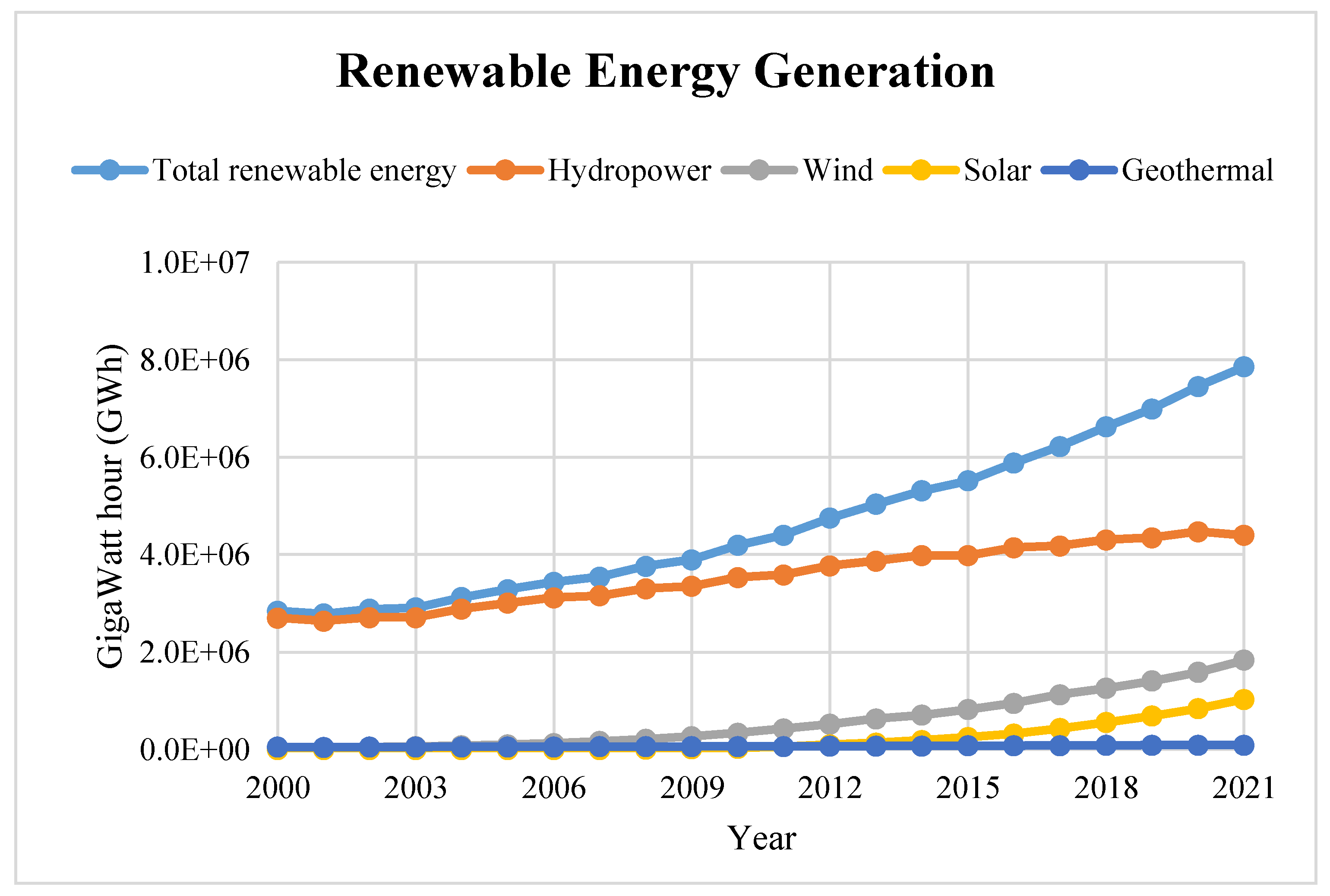
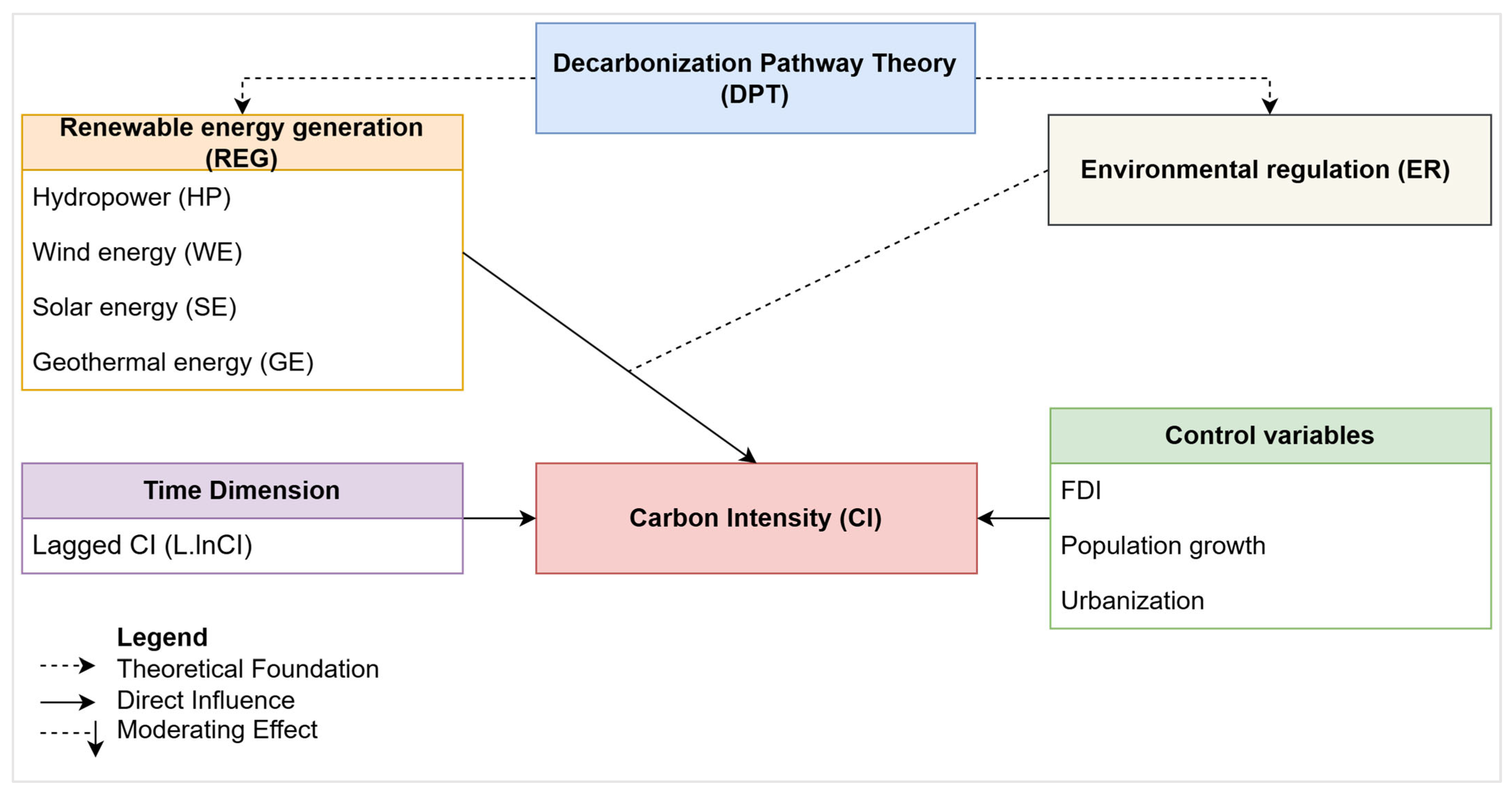

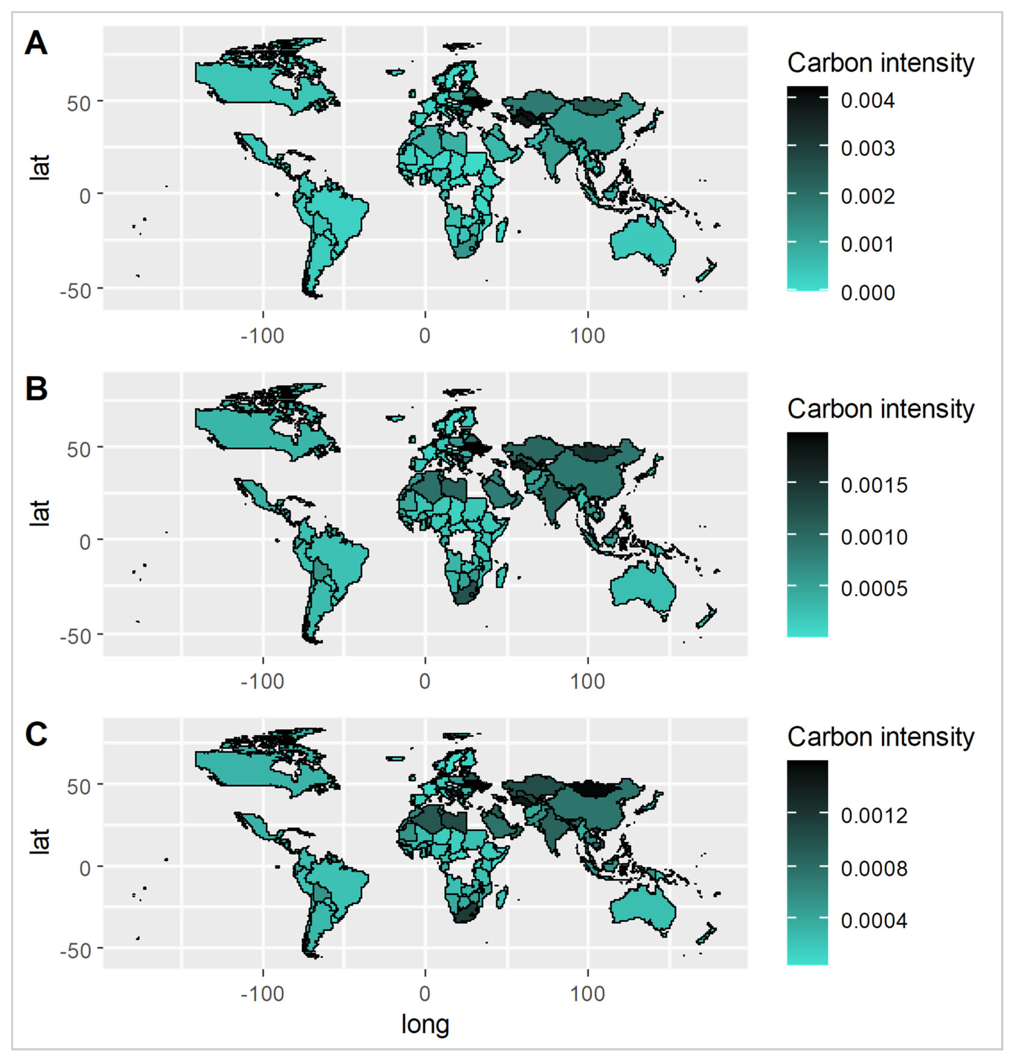
Disclaimer/Publisher’s Note: The statements, opinions and data contained in all publications are solely those of the individual author(s) and contributor(s) and not of MDPI and/or the editor(s). MDPI and/or the editor(s) disclaim responsibility for any injury to people or property resulting from any ideas, methods, instructions or products referred to in the content. |
© 2025 by the authors. Licensee MDPI, Basel, Switzerland. This article is an open access article distributed under the terms and conditions of the Creative Commons Attribution (CC BY) license (https://creativecommons.org/licenses/by/4.0/).