Theory of Quantity Value Traceability of Effective Apparent Power and Evaluation Method of Uncertainty

Abstract

Apparent power and power factor are crucial metrics for evaluating the energy transmission efficiency and reactive power management in power systems. The increasing complexity of power load structures, driven by evolving energy production and consumption models, has intensified the nonlinear and unbalanced characteristics of circuits, presenting significant challenges to accurate apparent power measurement. The IEEE 1459-2010 standard introduces the concept of effective apparent power to enhance the assessment of energy transmission efficiency under non-sinusoidal and unbalanced conditions. However, the absence of a physical standard and a standardized traceability method for effective apparent power results in inconsistent measurement outcomes across instruments. This study proposes a novel method to trace effective apparent power measurements to the International System of Units (SI) benchmarks, based on the loss characteristics of transmission lines. The method includes a comprehensive analysis of measurement uncertainty. Simulation and experimental validation confirm that the proposed traceability circuit can achieve a measurement uncertainty of 0.0110% (coverage factor k = 2), satisfying the engineering requirement of expanded uncertainty U approximately 0.02% (k = 2). These results demonstrate the method’s practical suitability for engineering applications.

1. Introduction

The integration of new energy sources and power electronic devices into the power grid has significantly increased the complexity of load conditions, characterized by load imbalances, intensified voltage fluctuations, elevated harmonic content, and increased reactive power [1,2,3,4,5,6]. These factors contribute to higher circuit losses and, nowadays, power quality issues have attracted increasing global attention. IEC 61000-4-30 defines the measurement grades (A, S, B) for power quality parameters and specifies the performance requirements for monitoring equipment [7]. The European Union’s voltage quality standards for public power supply systems clearly stipulate the limits for voltage deviation, fluctuation, harmonics, etc., and require power suppliers to ensure compliance with the standards at the Point of Common Coupling (PCC) [8]. In most countries, grid operators integrate the power factor into the power adjustment tariff coefficient [9,10], applying additional fees to high-consumption users to incentivize the implementation of power factor correction measures. In some regions of North America, however, grid management companies directly bill consumers based on apparent power (kVA) rather than active power (kWh). These strategies collectively aim to minimize transmission line losses and enhance power quality [11,12]. Consequently, as a central technical metric for power quality, the traceable measurement of power factor has grown increasingly critical. This fundamentally hinges on the traceability of apparent power (kVA) measurements—the core determinant of power factor accuracy.

After extensive debate spanning over a century, the method proposed by A.E. Emanuel in 1995 for decomposing apparent power in three-phase unbalanced nonlinear circuits gained widespread acceptance and was adopted into the IEEE 1459-2010 standard [13]. Among these, only $P_1^{+}$ represents an “expected” power component, while the remaining components contribute to “unexpected” active power losses in transmission lines, leading to the inefficient use of electrical resources.

Drawing on the physical mechanism of the Poynting vector power flow, A.E. Emanuel’s derivation of apparent power [13] offers a more precise description of “unexpected” power components in three-phase nonlinear unbalanced circuits compared to the definitions proposed by C.I. Budeanu (1927), M. Depenbrock (1960), and L.S. Czarnecki (1984) [14,15,16]. Emanuel’s definition exhibits a smaller deviation from actual conditions.

According to IEEE 1459-2010, in unbalanced three-phase circuits, non-active power—stemming from unbalanced energy oscillations across the three phases and the neutral line—induces active power losses, leading to a power factor below unity. Consequently, when three-phase load voltage or current is unbalanced, the ideal economic operating condition of minimal loss (power factor = 1) cannot be achieved.

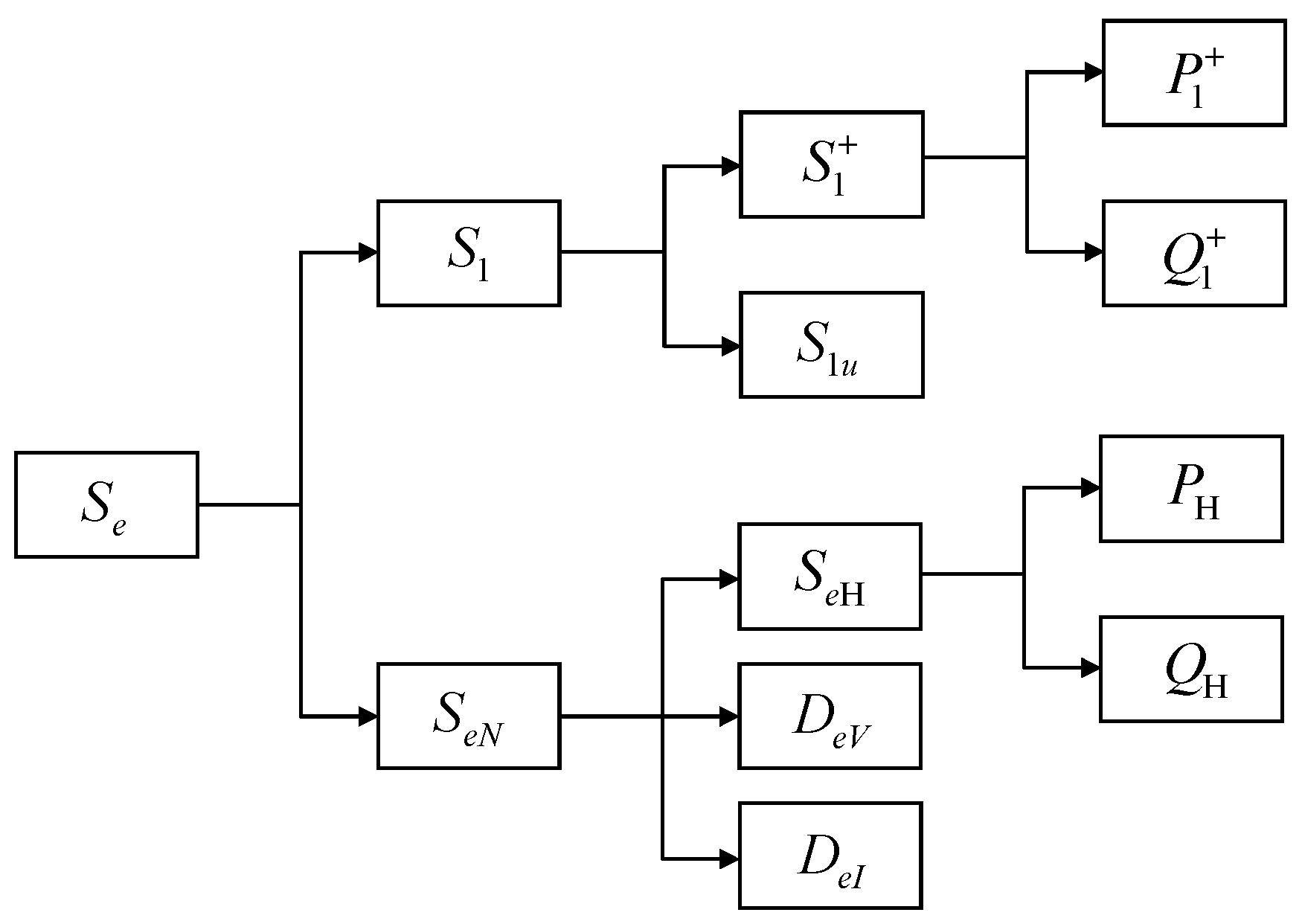
The power tree of IEEE 1459-2010 can be represented by Figure 1. The power decomposition framework defined in IEEE 1459-2010 (illustrated in Figure 1) represents the state of the art in modern power theory. Unlike traditional approaches that rely on simplified scalar power definitions, this standard provides a comprehensive decomposition of apparent power into its fundamental and non-fundamental components, including active, reactive, harmonic distortion, and unbalance terms. This advanced methodology enables more accurate quantification of power quality issues, facilitates precise loss allocation in power systems, and supports optimal compensation strategies. Its rigorous formulation aligns with contemporary grid challenges, such as renewable energy integration and nonlinear loads, making it the preferred reference for both industrial applications and power quality research.

The traceability of measurement results is fundamental to all measurement and analysis activities. For measurement results from different instruments to be comparable, they must be evaluated on a consistent scale. While the measurement formula for single-phase apparent power is universally accepted, the lack of a standardized definition for three-phase circuits leads to inconsistent measurement outcomes. Among the three widely accepted definitions of apparent power—arithmetic (Sₐ), vector (Sᵥ), and effective (Sₑ)—their calculation methods differ significantly. IEEE 1459-2010 employs a geometric analysis to evaluate the arithmetic and vector definitions, ultimately advocating for their discontinuation in favor of the effective apparent power (S_e). The rationale lies in Sₑ’s unique treatment of the three-phase system as a unified energy conversion entity, rather than three separate circuits, ensuring consistency with actual transmission losses.

Crucially, $S_e^2$ exhibits a proportional relationship with line losses, making it invaluable for loss quantification and energy efficiency optimization, particularly when neutral line zero-sequence currents contribute to economically significant losses [17,18,19]. If the primary objective of apparent power measurement is to “precisely evaluate line losses and maximize active power delivery” [20,21], effective apparent power (Sₑ) emerges as the most suitable definition, offering a more objective and physically meaningful representation of system-wide losses.

NEMA C12.31-2024 introduces three new apparent power definitions, providing their time-domain formulas and frequency-domain measurement models —fundamental apparent power, apparent power with DC component, and apparent power without DC component. For multi-cycle signals, average approximation methods are also specified. While these definitions and models are practical, they lack feasible measurement traceability methods [22]. Reference [23] proposes a traceability approach for arithmetic, vector, and effective apparent power based on measurement formulas. However, when the underlying assumptions of these formulas fail, both standard and instrument-measured values may yield identical but “unreasonable” results, deviating from the intended measurement objectives. For example, in a three-phase four-wire circuit with only Phase A carrying load current, the three apparent power definitions produce distinct results.

Given the advantages of effective apparent power (Sₑ) in quantifying transmission line losses and the absence of robust traceability methods, this paper proposes a traceability framework for Sₑ to physical quantity standards, including an uncertainty evaluation approach. This framework enables apparent power instruments, designed to “assess and optimize transmission line utilization efficiency” [24,25], to achieve traceability to International System of Units (SI) benchmarks. Simulation and experimental results confirm that the proposed method accurately reflects line losses and ensures SI-compliant traceability.

2. Effective Apparent Power Quantity Traceability Model to SI Standards

The definition and decomposition of apparent power are closely aligned with its original design purposes. This paper first establishes the following two measurement models.

Measurement Model 1: Based on the law of conservation of energy, the transmission line loss, ΔW, is defined as the difference between the active electrical energy measured at the power supply side, W_source, and that received at the load side, W_load. Given that the active power associated with line losses is linearly additive in the time domain, Equation (1) is derived as follows:

$$∆W=W_{source}-W_{load}$$

(1)

Measurement Model 2: Assuming that the line impedance parameter R_s remains constant (neglecting the skin effect and proximity effect under high-order harmonics), according to the definition of effective apparent power, S_e = V_eI_e (where I_e is the effective current, taking single-phase system as an example here), the line loss can be determined using the measured values of the load’s effective apparent power S_e and the effective voltage V_e within the measurement interval. This leads to the derivation of Equation (2).

$$∆W=R_s{(S_e/V_e)}^{2}T$$

(2)

In Equation (2), R_s represents the line impedance, S_e denotes the effective apparent power, V_e indicates the effective voltage, and T signifies the total measurement time. Combining Equations (1) and (2), it is evident that the right-hand sides of the two equations are equal. After rearrangement, the expression derived for S_e is shown in Equation (3):

$$S_e=V_e\sqrt{{\displaystyle \frac{W_{source}-W_{load}}{R_{s}T}}}$$

(3)

Let S be the reading of the apparent power instrument to be traced, subtract S_e from S, and then the error model of the apparent power instrument is shown in Equation (4):

$$∆S=S-V_e\sqrt{{\displaystyle \frac{W_{source}-W_{load}}{R_{s}T}}}$$

(4)

Since the derived expression of the effective apparent power S_e described by Equation (3) differs from its definition formula, to distinguish them, let the latter term on the right-hand side of Equation (4) be defined as S_r, as shown in Equation (5). When S_r is adopted as the standard measurement result, the measurement deviation of the instrument is given by ΔS.

$$S_r=S_e=V_e\sqrt{{\displaystyle \frac{W_{source}-W_{load}}{R_{s}T}}}$$

(5)

A single-phase effective apparent power traceability circuit is designed, as shown in Figure 2.

In the traceability circuit, the values of V_e (in volts, measured by a customized voltmeter), W_source (in joules, measured by a high-precision electricity meter), W_load (in joules, measured by a high-precision electricity meter), R_s (in ohms, using a standard resistor), and T (in seconds) are traceable to the corresponding International System of Units benchmarks. Consequently, this measurement circuit enables the traceability of the apparent power measurement result S for the single-phase apparent power instrument. To ensure compliance with the law of conservation of energy, the measurement uncertainty introduced by the power consumption of the electricity meters must be considered when necessary. This uncertainty can be mitigated by increasing the resistance value of the standard resistor R_s.

The uncertainty of the measurement equations can be evaluated using either the Guide to the Expression of Uncertainty in Measurement (GUM) method or the Monte Carlo method.

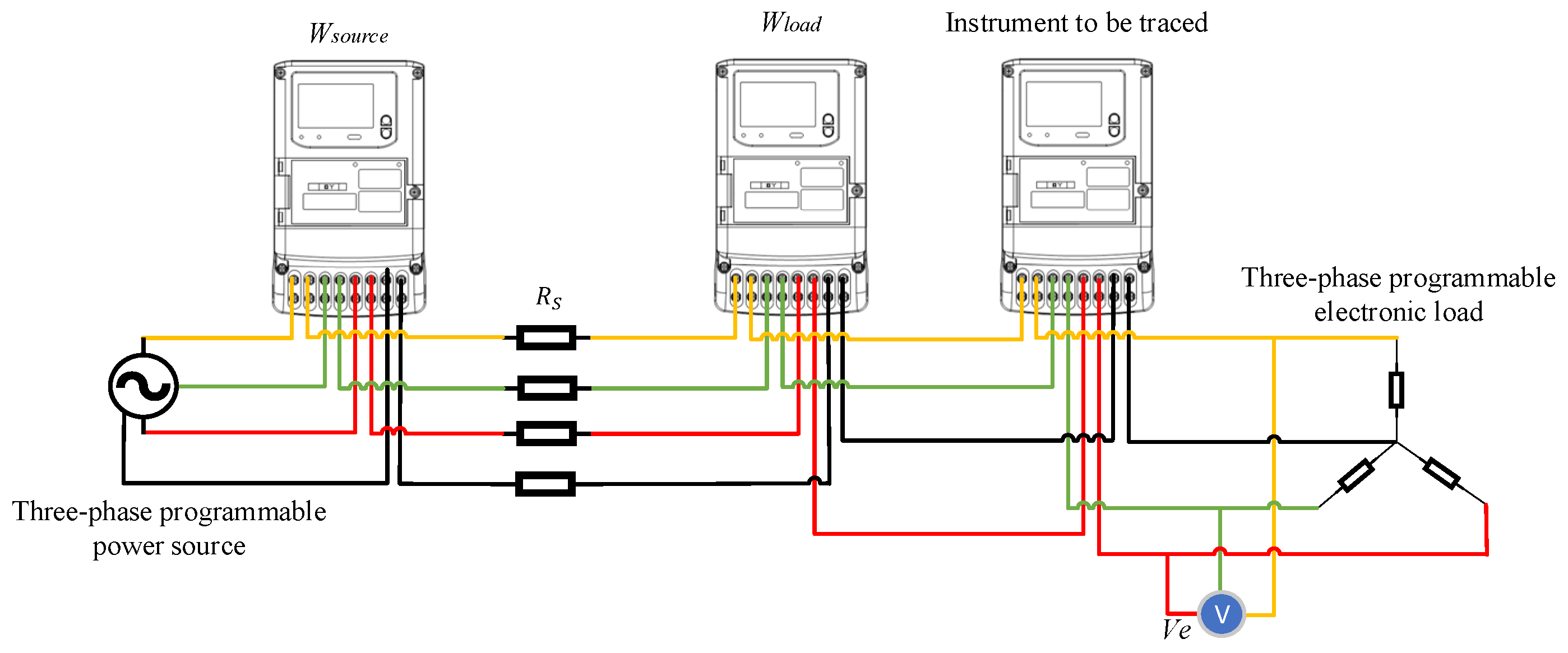
The design of the three-phase traceability circuit is presented in Figure 3 and Figure 4. It should be noted that the three-phase three-wire electricity meter is simplified and marked according to the direct connection mode.

The uncertainty evaluation method for the three-phase traceability circuit is analogous to that of the single-phase traceability circuit. Both the Guide to the Expression of Uncertainty in Measurement (GUM) method and the Monte Carlo method can be utilized for this evaluation. In the three-phase effective apparent power traceability models described above, the circuit’s voltage signal is controlled by a programmable power source, while the load is a programmable electronic load. By configuring the programmable power source and electronic load, various unexpected power signals can be generated as required, enabling the traceability of the effective apparent power to SI standards.

3. Simulation Verification

3.1. Under Ideal Standard Instrument Conditions

Using the three-phase four-wire effective apparent power traceability circuit depicted in Figure 4, the simulation experiment incorporates harmonic test waveforms specified for electric vehicle loads in OIML G22. Each phase of the three-phase programmable power supply outputs a harmonic voltage with a fundamental amplitude of 220 V at 50 Hz and harmonic components up to the 39th harmonic, as detailed in

Table 1. Harmonic components and contents.

Harmonic Number	Amplitude (%)	Harmonic Number	Amplitude (%)
1	100.00	2	0.25
3	3.00	4	0.20
5	2.40	6	0.16
7	2.28	8	0.15
9	2.16	10	0.14
11	2.05	12	0.00
13	1.95	14	0.00
15	1.85	16	0.00
17	1.76	18	0.00
19	1.67	20	0.00
21	1.59	22	0.00
23	1.51	24	0.00
25	1.43	26	0.00
27	1.36	28	0.00
29	1.29	30	0.00
31	1.23	32	0.00
33	1.17	34	0.00
35	1.11	36	0.00
37	1.05	38	0.00
39	1.00	40	0.00

. The standard resistor is set to 1 Ω. The three-phase programmable electronic load is configured as balanced, with fundamental currents of 0.1 A, 0.3 A, 0.5 A, 0.7 A, 0.9 A, and 1 A per phase. The harmonic components and their amplitudes for the current are identical to those of the voltage, as specified in Table 1. The measurement duration, T, is set to 1000 s. Under these conditions, the simulation results for ideal standard instruments are presented in

Table 2. Simulation results of the three-phase four-wire effective apparent power traceability circuit—Under Ideal Standard Instrument Conditions.

	0.1 A	0.3 A	0.5 A	0.7 A	0.9 A	1 A
S/VA	66.5918	199.5874	332.3323	464.8267	597.0706	663.0988
Ve/V	220.5437	220.3417	220.1397	219.9377	219.7357	219.6348
Wsource/J	6.6387 × 104	1.9916 × 105	3.3193 × 105	4.6470 × 105	5.9747 × 105	6.6385 × 105
Wload/J	6.6357 × 104	1.9889 × 105	3.3117 × 105	4.6321 × 105	5.9501 × 105	6.6081 × 105
Sr/VA	66.5918	199.5874	332.3323	464.8267	597.0706	663.0988

.

Additionally, a simulation verification of an unbalanced load test is conducted. The test conditions remain identical to those in Table 2, except that the three-phase programmable electronic load is adjusted to an unbalanced configuration. Specifically, phase C has no load current, while the currents in phases A and B remain unchanged from the balanced load test in Table 2. The results of the unbalanced load test are presented in

Table 3. Simulation results of the three-phase four-wire effective apparent power traceability circuit (under imbalanced load conditions)—Under Ideal Standard Instrument Conditions.

	0.1 A	0.3 A	0.5 A	0.7 A	0.9 A	1 A
S/VA	66.4155	198.9441	331.0719	462.8020	594.1370	659.6573
Ve/V	220.5774	220.4432	220.3094	220.1762	220.0433	219.9771
Wsource/J	4.4248 × 104	1.3268 × 105	2.2104 × 105	3.0931 × 105	3.9751 × 105	4.4158 × 105
Wload/J	4.4218 × 104	1.3241 × 105	2.2029 × 105	3.0784 × 105	3.9508 × 105	4.3858 × 105
Sr/VA	66.4155	198.9441	331.0719	462.8020	594.1370	659.6573

.

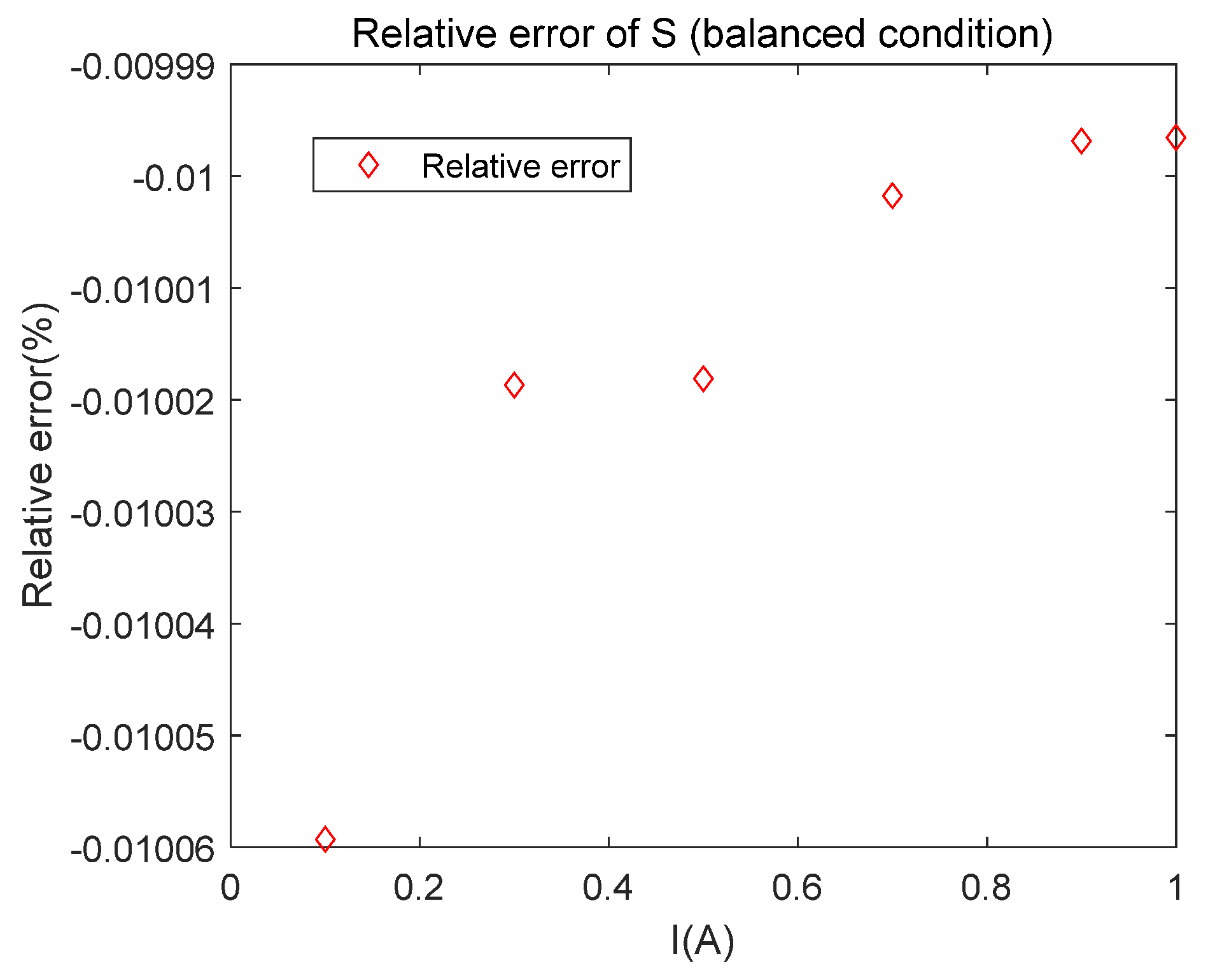
We compare the values of S and S_r under various load current conditions, and the results are shown in Figure 5 and Figure 6.

By analyzing Figure 5 and Figure 6, it can be seen that, in the case of ideal standard instruments, regardless of whether the system is in a balanced state or an unbalanced state, there is no error between the value of S and the ideal value S_r. This indicates that the traceability method proposed in this paper is practical and feasible, and that the measured value S can be traced back to the International System of Units benchmarks from the theoretical true value S_r.

3.2. Under Non-Ideal Standard Instrument Conditions

Following the validation of the traceability model’s feasibility using an ideal standard instrument, instrument errors were introduced to the ideal standard instrument to simulate the performance of an actual traceability system.

In the three-phase programmable power supply, each phase still outputs harmonic voltages containing up to the 39th harmonic. The specific harmonic components and their contents are shown in Table 1, with the fundamental voltage being 220 V. The standard resistor is set to 1 Ω. The three-phase programmable electronic load is balanced, and the balanced three-phase fundamental currents are still set to 0.1 A, 0.3 A, 0.5 A, 0.7 A, 0.9 A, and 1 A. The harmonic components and their contents are consistent with those of the voltage, as shown in Table 1. Two high-precision electric energy meters, calibrated against common high-precision standard electric energy meters, were used, with an error level of 0.05%. The standard resistor exhibited an error level of 0.05%. A customized voltmeter, employed to measure the effective voltage, had a voltage error level of 0.01%. The measurement duration, T, was set to 1000 s. Under these conditions, the simulation results for non-ideal standard instruments are presented in

Table 4. Simulation results of the three-phase four-wire effective apparent power traceability circuit—Under Non-Ideal Standard Instrument Conditions.

	0.1 A	0.3 A	0.5 A	0.7 A	0.9 A	1 A
S/VA	66.5984	199.6070	332.3647	464.8716	597.1279	663.1620
Ve/V	220.5657	220.3635	220.1614	219.9593	219.7573	219.6562
Wsource/J	6.6400 × 104	1.9920 × 105	3.3200 × 105	4.6479 × 105	5.9759 × 105	6.6398 × 105
Wload/J	6.6370 × 104	1.9893 × 105	3.3124 × 105	4.6330 × 105	5.9512 × 105	6.6094 × 105
Sr/VA	66.6051	199.6270	332.3980	464.9181	597.1876	663.2283

.

A simulation-based validation of the unbalanced load test was conducted. The experimental conditions were consistent with those specified in Table 4, except for the configuration of the three-phase programmable electronic load, which was adjusted to an unbalanced state. Specifically, the load current in phase C was set to zero, while the currents in phases A and B remained identical to those in the test conditions of Table 4. The results of the simulation are presented in

Table 5. Simulation results of the three-phase four-wire effective apparent power traceability circuit (under imbalanced load conditions)—Under Non-Ideal Standard Instrument Conditions.

	0.1 A	0.3 A	0.5 A	0.7 A	0.9 A	1 A
S/VA	66.4221	198.9636	331.1040	462.8463	594.1932	659.7194
Ve/V	220.5994	220.4651	220.3313	220.1979	220.0650	219.9988
Wsource/J	4.4257 × 104	1.3271 × 105	2.2108 × 105	3.0938 × 105	3.9759 × 105	4.4167 × 105
Wload/J	4.4227 × 104	1.3244 × 105	2.2033 × 105	3.0790 × 105	3.9516 × 105	4.3867 × 105
Sr/VA	66.4287	198.9835	331.1371	462.8626	594.2527	659.7853

.

The values of S and S_r were compared under various load current conditions. The results are presented in Figure 7 and Figure 8.

As shown in Figure 7 and Figure 8, when non-ideal standard instruments are used, a discrepancy exists between the measured value of S and the ideal value S_r. The error, ΔS, is calculated using Equation (4). Additionally, the measured value S can be traced to the International System of Units (SI) standards through S_r.

The simulation results demonstrate that the traceability model proposed in this study is applicable to circuits with non-ideal standard instruments and offers significant practical value.

4. The Practical Implementation of the Traceability Mode

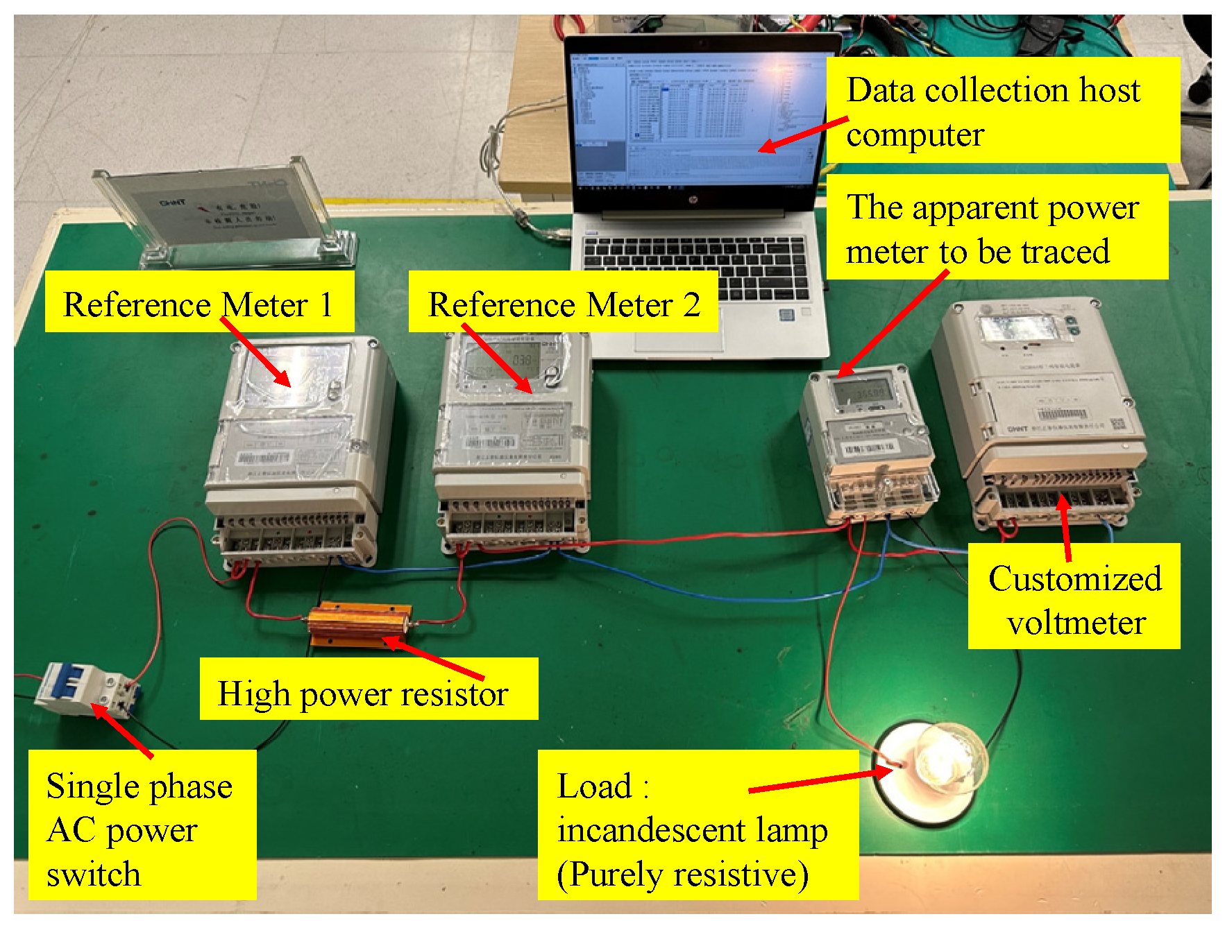
Simulation verification confirms that the proposed traceability model for effective apparent power is both reasonable and feasible. The model enables traceability to the International System of Units (SI) by comparing the measured apparent power S, obtained from the instrument under test, with the theoretical true value S_r. Using the single-phase effective apparent power traceability circuit as an example, the practical implementation of the traceability model is illustrated in Figure 9.

The traceability circuit illustrated in Figure 9 is designed to facilitate the accurate measurement and traceability of single-phase equivalent apparent power. A detailed description of each component in the circuit is provided below to clarify their roles and specifications.

Voltage Source: The circuit employs a stable single-phase 220 V (rms) voltage source operating at 50 Hz, provided by a laboratory-grade power supply. This source is calibrated to maintain a voltage stability within ±0.1% to ensure consistent excitation of the circuit, minimizing fluctuations that could affect measurement accuracy.

Reference Meters: Two high-accuracy energy meters, manufactured by a reputable Chinese energy meter company, are positioned at the power supply and load ends of the circuit. These meters, designated as Reference Meter 1 (supply end) and Reference Meter 2 (load end), have a specified measurement error of less than 0.04% for active power. Both meters are capable of measuring voltage, current, and power, with a resolution of 0.001 kWh for energy measurements. They are calibrated against national standards to ensure traceability to the International System of Units (SI).

Apparent Energy Meter (Under Traceability): The apparent energy meter to be traced is an independently developed device by a Chinese energy meter company. This meter is designed to measure apparent power based on the effective apparent power theory. Its nominal input range is 220 V and up to 60 A, with a specified accuracy of ±2% for apparent power measurements. The meter is interfaced with the circuit to evaluate its performance against the reference measurements provided by the traceability setup.

Line Impedance: A customized 20 Ω high-power resistor is used to simulate the line impedance. This resistor is engineered with a temperature drift of less than 15 ppm/°C to maintain stable resistance under varying thermal conditions. The resistor is rated to handle power dissipation up to 100 W, ensuring reliable operation across the range of test currents. Its precise resistance value is verified using a calibrated high-accuracy ohmmeter prior to testing.

Customized Voltagemeter: A specialized equivalent voltage meter is employed to measure the effective voltage, which is critical for calculating the equivalent apparent power. This meter has a measurement range of 0–250 V and an accuracy of ±0.01%. For enhanced precision, an eight-and-a-half-digit digital multimeter or a standard digital multimeter with an accuracy of ±0.01% can be substituted if available. The meter is configured to sample voltage at a rate of 6400 samples per second to capture steady-state conditions accurately.

Load: The load consists of pure resistive incandescent lamps, selected for their stable resistive characteristics and minimal harmonic distortion. The lamps are available in multiple power ratings, allowing the load current to be adjusted by varying the lamp model or quantity. The total load current is controlled within the range of 0.1 A to 60 A to simulate realistic operating conditions. The lamps are connected in parallel to ensure uniform voltage distribution.

Communication Interface: All measurement instruments (energy meters, apparent energy meter, and equivalent voltage meter) are equipped with RS-485 communication interfaces ensuring reliable and synchronized data acquisition at a baud rate of 9600 bps. These interfaces enable real-time data transmission to a computer-based upper control system, which records and processes the measurements.

The single-phase equivalent apparent power traceability circuit, configured with the above components, is used for field tests. To ensure measurement reliability, data recording commences only after the incandescent lamps reach thermal stability, typically after a warm-up period of 5 min. The power consumption of Energy Meter 2 is accounted for in the data analysis to avoid systematic errors. The measurement duration for each test is set to 1 h, with data sampled at 10 s intervals. The resulting test data are presented in

Table 6. Experimental results of the single-phase effective apparent power traceability circuit.

	0.1937 A	0.3776 A	0.6556 A
Reading of the apparent power meter to be traced (S)/VA	43.7839	84.1230	142.1088
Reading of the voltage meter (Ve)/V	226.0400	222.7833	216.9600
Energy consumed of Reference Meter 1 (Wsource)/kWh	0.0463	0.0890	0.1527
Energy consumed of Reference Meter 2 (Wload)/kWh	0.0446	0.0852	0.1431
Power consumption of reference meter/W	0.9640	0.9640	0.9640
Sr/VA	43.3620	83.8920	142.5677

.

Analyzing the data in Table 6, the test results are in line with expectations. The value of S has a small error from the ideal value S_r, as shown in Figure 10 below.

Furthermore, the success of the single-phase experiment supports the feasibility of the three-phase traceability circuit, as the core principles of apparent power measurement and traceability are consistent across both configurations.

5. Uncertainty Evaluation of the Measurement Results

In the proposed effective apparent power traceability model, the reference standard value S_r serves as the benchmark for traceability. The measured apparent power S from the instrument under test is compared against S_r to establish its traceability to the International System of Units (SI). The reliability of this traceability hinges on the uncertainty of S_r. Accordingly, the uncertainty evaluation for S_r is conducted as follows.

The primary sources of uncertainty for S_r in the traceability circuit model are identified through detailed analysis and include the following components: (1) measurement deviations of the source power W_source and load power W_load; (2) resistance tolerance of the standard resistor R_s; (3) measurement error of the custom voltmeter V_e; (4) timing error in the measurement duration T.

The measurement results for W_source and W_load are obtained using high-precision electricity meters. Consequently, the standard uncertainties, u(W_source) and u(W_load), are derived as Type B uncertainties based on the specifications provided in the meter’s documentation. Taking Reference Meter 1 and Reference Meter 2 in Figure 9 as examples, according to the specification sheet, their power energy error uncertainty under the power frequency of 50 Hz is 0.04%, which is assumed to follow a uniform distribution with a coverage factor of k = $\sqrt{3}$.

The measurement result of V_e is provided by a specially customized high-precision voltage meter, which is designed to give the effective value of all voltage signals within the measurement interval. The uncertainty Ve can be evaluated according to Type A standard uncertainty or using the Type B standard uncertainty result from its specification as a reference. Specifically, the measurement result of Ve is provided by a specially customized effective voltage meter, and its measurement uncertainty for 220 V AC voltage at 50 Hz is 0.01%, with a coverage factor of k = 2.

R_s is a customized high-accuracy, low-temperature-drift high-power aluminum-shell resistor designed to provide a stable resistance output. To neglect the influence of connection line impedance and improve measurement resolution, R_s can adopt a relatively larger value, and its Type B standard uncertainty u(R_s) is calculated based on data from calibration certificates or specification sheets. It should be noted that R_s must reach thermal stability during physical experiments. In the test shown in Figure 9, the temperature drift of this resistor does not exceed 15 ppm, and the typical uncertainty is 0.01% with a coverage factor of k = 2.

The time interval, T, is measured using a standard time base source, with its Type B standard uncertainty, u(T), derived from the data provided in the verification certificate. For example, a typical rubidium clock achieves an uncertainty in the order of 10⁻¹¹. Compared to other uncertainty components, the contribution of u(T) to the overall measurement uncertainty in the calculation model is generally negligible.

Additionally, the measurement uncertainty arising from the power consumption factor of the electricity meter should be evaluated when relevant. Using the GUM (Guide to the Expression of Uncertainty in Measurement) framework and applying the law of uncertainty propagation, the combined standard uncertainty of S_r is determined. The measurement model for S_r is given by Equation (5). As the input quantities are uncorrelated, the combined variance is expressed as Equation (6).

$${u_c^2(S}_r)={\left[{\displaystyle \frac{\partial S_r}{\partial W_{source}}}\right]}^2{u}^2\left(W_{source}\right)+{\left[{\displaystyle \frac{\partial S_r}{\partial W_{load}}}\right]}^2{u}^2\left(W_{load}\right)+{\left[{\displaystyle \frac{\partial S_r}{\partial V_e}}\right]}^2{u}^2\left(V_e\right)+{\left[{\displaystyle \frac{\partial S_r}{\partial R_s}}\right]}^2{u}^2\left(R_s\right)+{\left[{\displaystyle \frac{\partial S_r}{\partial T}}\right]}^2{u}^2\left(T\right)$$

(6)

The sensitivity coefficients are shown in Equations (7)–(11), respectively.

$${\displaystyle \frac{\partial S_r}{\partial W_{source}}}={\displaystyle \frac{V_e}{2\sqrt{{R_{s}T(W}_{source}-W_{load})}}}$$

(7)

$${\displaystyle \frac{\partial S_r}{\partial W_{load}}}={\displaystyle \frac{-V_e}{2\sqrt{{R_{s}T(W}_{source}-W_{load})}}}$$

(8)

$${\displaystyle \frac{\partial S_r}{\partial V_e}}=\sqrt{{\displaystyle \frac{W_{source}-W_{load}}{R_{s}T}}}$$

(9)

$${\displaystyle \frac{\partial S_r}{\partial R_s}}={\displaystyle \frac{-V_e}{2}}\sqrt{{\displaystyle \frac{W_{source}-W_{load}}{T}}}{R_s}^{-1.5}$$

(10)

$${\displaystyle \frac{\partial S_r}{\partial T}}={\displaystyle \frac{-V_e}{2}}\sqrt{{\displaystyle \frac{W_{source}-W_{load}}{R_s}}}{T}^{-1.5}$$

(11)

Taking the single-phase traceability circuit as an example, the combined standard uncertainty u_c(S_r) is calculated. By substituting the measurement data in Table 6 into Equations (6)–(11), the combined standard uncertainty u_c(S_r) and expanded uncertainty U (k = 2) are obtained, as shown in

Table 7. The uncertainty calculation results of the single-phase effective apparent power traceability circuit.

	0.1937 A	0.3776 A	0.6556 A
uc(Sr)/%	0.0055	0.0107	0.0181
U(k = 2)/%	0.0110	0.0213	0.0362

below.

As shown in Table 7, in the test results of the single-phase effective apparent power traceability circuit depicted in Figure 9, the expanded uncertainty U (k = 2) of S_r reaches 0.0110% when the load current is 0.1937 A, meeting the engineering application requirement that U (k = 2) is approximately 0.02%. The numerical differences in uncertainty calculation results under different current loads are mainly attributed to the variation in the sensitivity coefficient with the load current. The physical experiment shown in Figure 9 serves as a simplified demonstration to validate the feasibility of the proposed effective apparent power traceability circuit. To achieve lower measurement uncertainty, adjustments can be made to the values of T and R_s in the traceability model, or alternatively, higher-accuracy energy meters, voltmeters, and standard resistors available on the market may be utilized.

6. Conclusions

This study introduces a method for tracing the quantity value of apparent power based on the effective apparent power theory. Building on two measurement models for line losses, traceability circuit models for single-phase and three-phase effective apparent power are developed. The simulation test results demonstrate that the apparent power instrument to be traced can accurately measure the apparent power value in the circuit. Even in the case of a non-ideal instrument, the relative error between the reading S of the instrument to be traced and the ideal true value S_r can be maintained at a level of −0.01%. And this method accurately reflects line losses and enables traceability to the International System of Units (SI) standards. Compared to existing quantity value traceability methods defined by measurement equations, the proposed method better aligns with the original intent of effective apparent power, which is to quantitatively assess the actual losses in transmission lines. Furthermore, its applicability to complex circuits enhances its practical value.

The actual test results of the single-phase traceability circuit show that the maximum relative error between the reading S of the instrument to be traced and the ideal true value S_r occurs at the load point of 0.1937 A, reaching 0.9730%. An uncertainty evaluation based on the Guide to the Expression of Uncertainty in Measurement (GUM) method demonstrates that the proposed traceability circuit achieves an expanded uncertainty of 0.0110% (k = 2), meeting the engineering requirement of approximately 0.02% (k = 2). This method establishes a metrological traceability foundation for ‘effective apparent power,’ a critical line loss control indicator in modern power systems. By enabling collaborative power quality management between the grid and users, it maximizes transmission line utilization and minimizes energy losses.

Based on the foundation of this research paper, future studies will further explore the measurement traceability of apparent power in transient and dynamic processes. Meanwhile, given the rapid growth trend of nonlinear loads in power systems, it will be of great significance to study the measurement traceability methods for power factor and apparent power, as well as the line loss characteristics in systems with nonlinear loads. This research will help improve the power quality in power systems and ensure efficient energy utilization.

References

- Wang, L.; Tang, H. Research on electric energy measurement method of energy measurement instruments with unbalanced load. Electr. Switchg. 2024, 62, 65–68. [Google Scholar]
- Liu, H.R. Research on Control Strategy of Delta-Connected Multi-Level SVG under Unbalanced Load. Master’s Thesis, Anhui University of Technology, Ma’anshan, China, 2023. [Google Scholar]
- Hang, X.Q.; Wang, X.R.; Wang, D.L.; Zhang, L. On apparent power of unbalanced non-sinusoidal electric power system. Power Syst. Prot. Control. 2006, 12, 30–34. [Google Scholar] [CrossRef]
- Wang, X.; Chen, J.; Yuan, R.; Jia, X.; Zhu, M.; Jiang, Z. OOK power model based dynamic error testing for smart electricity meter. Meas. Sci. Technol. 2017, 28, 025015. [Google Scholar] [CrossRef]
- Gaiceanu, M.; Epure, S.; Solea, R.C.; Buhosu, R. Power Quality Improvement with Three-Phase Shunt Active Power Filter Prototype Based on Harmonic Component Separation Method with Low-Pass Filter. Energies 2025, 18, 556. [Google Scholar] [CrossRef]
- Ghanayem, H.; Alathamneh, M.; Yang, X.; Seo, S.; Nelms, R.M. Enhanced Three-Phase Shunt Active Power Filter Utilizing an Adaptive Frequency Proportional-Integral–Resonant Controller and a Sensorless Voltage Method. Energies 2025, 18, 116. [Google Scholar] [CrossRef]
- IEC 61000-4-30; 2015: Testing and Measurement Techniques—Power Quality Measurement Methods. IEC Technical Committee: Geneva, Switzerland, 2015.
- EN 50160:2010; Voltage Characteristics of Electricity Supplied by Public Distribution Systems. European Committee for Electro technical Standardization: Brussels, Belgium, 2010.
- Liao, T.; Zhang, J.F.; Zheng, J.H.; Wang, H.J.; Zhang, M.K. Principles and measures for distributed photovoltaic users to reduce power adjustment electricity charges. Pop. Util. Electr. 2023, 9, 16–17. [Google Scholar]
- Lai, J.H. Research on reactive power compensation of all cable power through-line for high-speed railway with power regulation fee. Master’s Thesis, Southwest Jiaotong University, Chengdu, China, 2022. [Google Scholar]
- Blasco, P.A.; Montoya-Mira, R.; Diez, J.M. Formulation of the phasors of apparent harmonic power: Application to Non-Sinusoidal three-phase power systems. Energies 2018, 11, 1888. [Google Scholar] [CrossRef]
- Li, X.P. Research on the calculation and allocation method of distribution network loss taking into account the effects of three-phase unbalance and harmonics. Master’s Thesis, Lanzhou Jiaotong University, Lanzhou, China, 2024. [Google Scholar]
- Emanuel, A.E.; Langella, R.; Testa, A. Power definitions for circuits with nonlinear and unbalanced loads—The IEEE standard 1459–2010. In Proceedings of the 2012 IEEE Power and Energy Society General Meeting, San Diego, CA, USA, 22–26 July 2012. [Google Scholar] [CrossRef]
- Budeanu, C.I. Puissances Reactives et Fictives; Romanian National Institute for Energy Research: Bucharest, Romania, 1927. [Google Scholar]
- Depenbrock, M. Investigation of Voltage and Power Conditions at Converters Without Energy Storage. Ph.D. Thesis, Technical University of Hanover, Hanover, Germany, 1962. [Google Scholar]
- Czarnecki, L.S. Orthogonal decomposition of the currents in a 3-phase nonlinear asymmetrical circuit with a nonsinusoidal voltage source. IEEE Trans. Instrum. Meas. 1988, 37, 30–34. [Google Scholar] [CrossRef]
- Emanuel, A.E. Apparent power definitions for three-phase systems. IEEE Trans. Power Deliv. 2022, 14, 767–772. [Google Scholar] [CrossRef]
- Zhao, L.H.; Niu, S.J.; Rong, Q.; Niu, C.C.; Feng, Z.S. Research on power factor measuring method in traction power supply system. Electr. Meas. Instrum. 2016, 53, 51–56+61. [Google Scholar] [CrossRef]
- Wang, S.W.; Liu, X.Z.; Xuan, S.; Mao, Q.; Yao, W.B. Research on apparent power and power factor calculation methods based on line loss equivalence. Electr. Meas. Instrum. 2024, 61, 65–70. [Google Scholar]
- Ferrero, A. Definitions of electrical quantities commonly used in non-sinusoidal conditions. Eur. Trans. Electr. Power 1998, 8, 235–240. [Google Scholar] [CrossRef]
- Willems, J.L.; Ghijselen, J.A.; Emanuel, A.E. The apparent power concept and the IEEE Standard 1459–2000. IEEE Trans. Power Deliv. 2005, 20, 876–884. [Google Scholar] [CrossRef]
- NEMA C12.31G-TR-2024; American National Standard for Electric Meters—Code for Electricity Metering. National Electrical Manufacturers Association: Rosslyn, VA, USA, 2024.
- Wang, T.T.; Cui, W.Q. An overview of algorithm traceability. Metrol. Sci. Technol. 2023, 67, 23–30. [Google Scholar] [CrossRef]
- Tian, M.X.; Zhao, Y.X.; Wang, J.B. Apparent power calculation based on equivalent scheme. Electr. Power Autom. Equip. 2017, 37, 153–158. [Google Scholar] [CrossRef]
- Zhao, Y.X. Analysis of IEEE Std 1459–2010 and research on its application in harmonic responsibility distinguish. Master’s Thesis, Lanzhou Jiaotong University, Lanzhou, China, 2017. [Google Scholar]
Figure 1.
Power tree of IEEE 1459-2010.
Figure 2.
Single-phase effective apparent power traceability circuit.
Figure 3.
Three-phase three-wire effective apparent power traceability circuit.
Figure 4.
Three-phase four-wire effective apparent power traceability circuit.
Figure 5.
Results of S and Sr under the balanced condition.
Figure 6.
Results of S and Sr under the imbalanced condition.
Figure 7.
Non-ideal instrument—measurement results under the balanced condition.
Figure 8.
Non-ideal instrument—measurement results under the imbalanced condition.
Figure 9.
Single-phase effective apparent power traceability circuit model.
Figure 10.
Measurement results of the single-phase traceability circuit.