Advanced Non-Unit Protection Strategy for MMC-HVDC Grids Leveraging Two-Dimensional High-Frequency Characteristics via HHT and SVM

Abstract

The rapid development of direct current (DC) grids poses significant challenges to the speed, reliability, and selectivity of fault protection systems. These systems are required to identify and distinguish between internal and external faults despite the constraints of limited information and time. This study introduces a non-unit protection scheme based on the classification of two-dimensional feature parameters utilizing the Hilbert–Huang transform (HHT) and a support vector machine (SVM). Through time–frequency analysis of the voltage waveform following DC faults, critical information within the high-frequency component of the fault voltage, specifically, the instantaneous frequency and amplitude of the wavefront, is extracted to distinguish internal from external faults. Two-dimensional feature parameters are associated with signal attenuation and distortion during fault propagation via the transmission path, thereby providing a foundation for precise fault identification. The employment of an SVM ensures the selectivity of this scheme without relying on protection settings. The efficacy of the scheme is validated through simulations conducted using PSCAD/EMTDC across various fault scenarios.

1. Introduction

DC grids based on modular multilevel converters (MMCs) are vital for high-power long-distance electricity transmission, enabling the seamless integration of new energy sources on a wide scale [1,2]. However, the low inertia and weak damping characteristics of flexible DC systems render them susceptible to severe fault currents [3]. The protection and restoration of DC faults are crucial for reliable operation and widespread development of DC grids [4,5]. To avoid damage to critical equipment within a flexible DC grid owing to DC faults, it is generally necessary to achieve fault clearance within 5 ms [6]. Therefore, fault detection and identification techniques for DC grids must shorten detection time and improve response sensitivity based on traditional detection and identification techniques [7,8].

The primary safeguard is often provided by local data to prevent transmission delays [9,10,11]. In their study, Chengyu Li et al. [12] provide a rapid approach for detecting short-circuit faults in HVDC grids. This approach relies on accurate measurement of the voltage across the current-limiting reactor under DC faults. Wang et al. [13] proposed a fault identification method based on the transient voltage square difference, which is used to identify faulted lines in an overhead line DC grid. Li et al. [14] proposed a protection scheme for multiterminal direct current (MTDC) systems in offshore wind farms. This scheme focuses on the detection of high-frequency components within fault current signals, enabling effective classification of fault categories and precise fault detection in every line. Traveling wave protection based on time-domain characteristics mainly uses numerical features, such as the voltage change rate and current change rate, to form criteria for identifying faults inside or outside the area [15,16]. Nevertheless, the rate of change and variation in the DC voltage and current significantly depend on the impedance of the long faulty line and grounding resistance [17]. Determining high-resistance faults and faults located at a great distance from an external fault using time-domain characteristics can be challenging [18]. The selectivity and dependability of methods that rely on them are constrained.

After a DC line fault occurs, a rapid change in the current can lead to a rapid change in the electromagnetic field, thereby triggering high-frequency voltage components [19]. Although excessive resistance may cause attenuation and distortion of high-frequency signals [20], its impact on high-frequency components is relatively small. Thus, high-frequency components can accurately indicate the propagation path of a DC fault [21]. By monitoring and analyzing the high-frequency components of surge voltages, it is possible to distinguish between internal and external faults and further determine the location and type of the fault [22,23,24]. Sabug Jr et al. [25] proposed a real-time boundary wavelet transform (RT-BWT) method to protect against DC faults in MTDC grids. Jayamaha et al. [26] utilized wavelet transform to capture the characteristic variations in current signals induced by network defects by sampling measured branch currents. Classification was performed using artificial neural networks, and the results demonstrated that the proposed method is capable of detecting and localizing defects quickly and independently. An approach that utilizes frequency-domain analysis substantially enhances selectivity. However, the complexity of the process of selecting the wavelet basis function reduces WT adaptability.

The Hilbert–Huang transform (HHT) developed by Norden E. Huang offers a powerful time–frequency analysis solution for analyzing nonlinear and nonstationary signals [27,28]. In [29], the performances of wavelet transform and Hilbert–Huang transform (HHT) in extracting fault features of high-voltage direct current transmission systems were compared. It was pointed out that wavelet transform requires repeated debugging of the basis functions and has a weak effect in extracting DC fault features. Compared with wavelet transform, HHT, as an adaptive time–frequency analysis method, does not require preset basis functions. It can adaptively extract signal modes through empirical mode decomposition. The fault features extracted by it are more obvious and can dual-locate the start and end points of faults. In terms of signal adaptability, HHT does not require preset basis functions and is adapted to the nonlinear characteristics of DC faults. In terms of time–frequency resolution, HHT can adaptively adjust to accurately capture transient high-frequency components. In terms of anti-noise ability, the combination of HHT and the improved technology has a better effect in suppressing modal aliasing and noise. In terms of the applicability of DC power grids, HHT is specifically designed for non-stationary signals and has a stronger ability to distinguish high-frequency characteristics of DC faults. Li et al. [30] examined the viability of using HHT to identify faults in HVDC systems based on voltage source converters (VSC). Feature extraction is achieved by using HHT in [31,32,33], and corresponding fault detection methods are proposed for HVDC systems. However, there is a dearth of studies on the use of HHT to safeguard DC grids from faults. In this study, the equivalent impedance values of DC fault voltage propagation paths at different locations were compared at different frequencies. It was found that the high-frequency components of the internal and external DC fault voltages are different. By employing the HHT to decompose the DC surge voltage, the high-frequency component’s frequency-domain characteristics of the voltage under different fault locations were analyzed. This method enables the extraction of the instantaneous frequency and amplitude, providing essential characteristic quantities for fault detection. The effects of fault distance, fault ground resistance, and the current-limiting reactor (CLR) on the frequency domain characteristics were then studied.

With these characteristic quantities, a fault-detection strategy for DC fault identification and classification in MTDC systems based on support vector machines (SVMs) is proposed. As a supervised learning algorithm, a support vector machine (SVM) maps input features to a high-dimensional space through kernel functions and can effectively achieve the linear partitioning of complex nonlinear patterns. This characteristic makes it particularly suitable for the fault identification task in this paper, because the instantaneous frequency and amplitude features extracted through the Hilbert–Huang transform (HHT) present complex nonlinear correlations between internal faults and external faults. This fault detection technique does not rely on telecommunication and demonstrates robust resistance to interference as well as excellent sensitivity and selectivity in identifying faults that are far away and problems with high-resistance grounding, making it a superior choice for reliable fault detection.

The remainder of this paper is organized as follows. Section 2 investigates the frequency-domain characteristics of the DC voltage in the context of DC failures. A DC fault detection approach utilizing support vector machines (SVMs) is presented in Section 3. Section 4 examines the elements that determine high-frequency features and subsequently tests the proposed solutions using simulations in PSCAD/EMTDC. Section 5 provides concluding remarks.

2. Transient Voltage Characteristics of Internal and External Faults

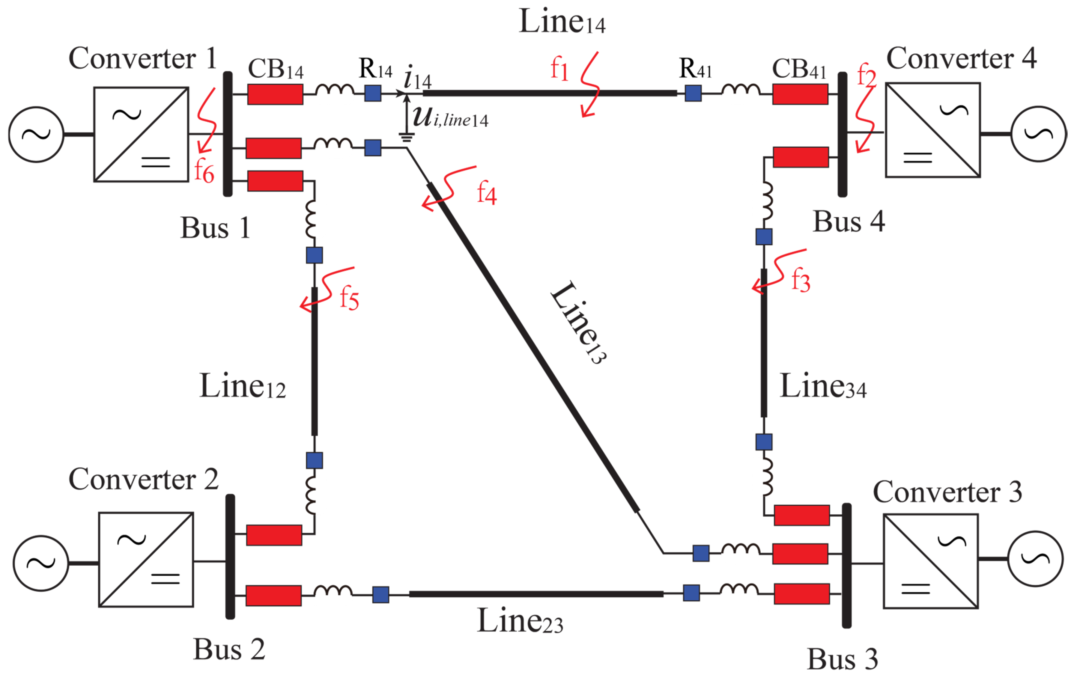
Figure 1 illustrates a typical standard topology of a four-terminal HVDC grid. Four modular multilevel converters (MMCs) are interconnected by high-voltage DC cables. Each cable connection is equipped with series DC circuit breakers (CBs) at both ends, which are crucial for the rapid isolation of faulty sections to avert cascading failures. Furthermore, current-limiting reactors (CLRs) are connected in series with the circuit breakers, effectively suppressing the rapid rise of fault currents during internal line faults. The relay, connected in series with the reactor and positioned on the inner side of the line, measures local signals to detect faults. In the event of an internal fault, it provides tripping signals to the circuit breakers on the same line. Regarding DC line fault detection based on local measurements by the protective relay, the challenge lies in differentiating between internal and external faults, particularly when the faults originate from the same direction.

Existing time-domain feature-based fault-detection schemes employ current and voltage derivatives to distinguish internal faults. When the value of the extracted feature exceeded the threshold value, an internal fault was considered. However, owing to the rapid attenuation of fault waves, selectivity cannot be ensured when distinguishing between internal high-resistance faults, internal far-terminal faults, and external metallic faults. The attenuation and distortion of the traveling waves under the combined effect of the grounding resistance, line impedance, and current-limiting reactor makes fault detection difficult.

However, it should be noted that the influences of the grounding resistance, line impedance, and current-limiting reactor on fault-traveling waves are different in the frequency domain. The distributed parameters of the DC line change at different frequencies, whereas the current limiter reactor exhibits an obvious filtering effect on the high-frequency components. Hence, it is important to investigate the transient properties of high-frequency elements in both internal and external problems. In pursuit of this objective, this section examines the frequency characteristics of voltage-traveling waves during DC faults and suggests techniques for extracting transient frequency-domain attributes using HHT.

2.1. Frequency-Domain Response

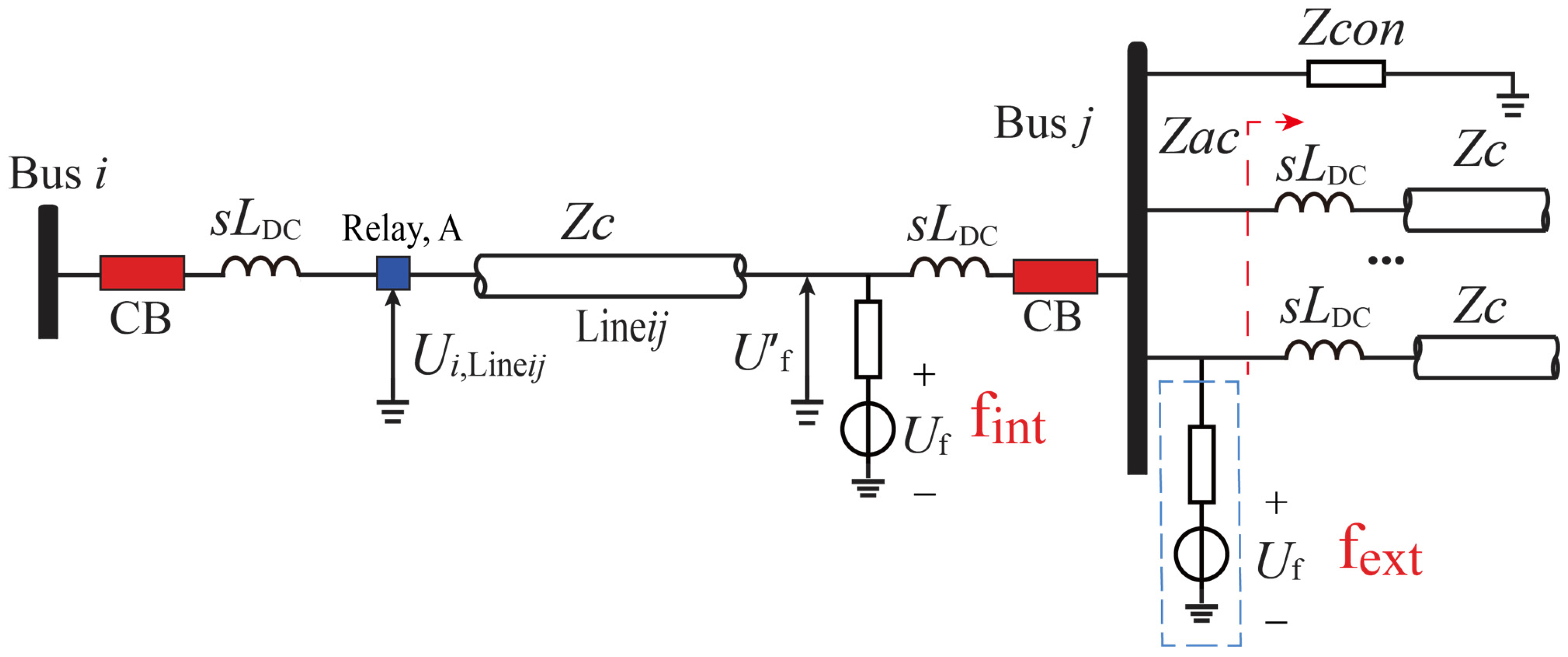
Taking any line Line_ij in the DC grid as an example, as depicted in Figure 2, when a DC line fault occurs, the voltage wave propagates along the transmission line and is subsequently recorded by relay A at the measurement point in the head of the line. The fault identification result dictates the operation of the circuit breaker located at the line head. Faults occurring within the reactors on both sides of the line are classified as internal faults, whereas those occurring beyond these boundaries are categorized as external faults.

The propagation process of the impulse voltage generated at the DC fault point to relay A can be divided into two parts: (1) an additional voltage source is generated at the grounded fault point and (2) the voltage traveling wave propagates to the detecting point along the transmission line. The incident traveling voltage wave measured by relay A can be formulated as follows:

$$U_{\mathrm{a}}(s)=U_{\mathrm{f}}^{\prime }(s)e^{-r\left(s\right)l}$$

(1)

where $U_{\mathrm{f}}^{\prime }(s)$ denotes the additional voltage at fault point. To simplify the calculation, the waveform distortion, attenuation, and propagation delay information are decoupled as follows:

$$A(s)=e^{-r\left(s\right)l}\approx {\displaystyle \frac{K_{\mathrm{a}}}{1+s{T}_{\mathrm{a}}}}{\mathrm{e}}^{-{\displaystyle \frac{sl}{v}}}$$

(2)

where $e^{-r\left(s\right)l}$ is the time delay of traveling wave propagation, v is the maximum speed of the traveling wave within the considered frequency range, l is the propagation distance, ${\displaystyle \frac{K_{\mathrm{a}}}{1+s{T}_{\mathrm{a}}}}$ represents the transmission attenuation and distortion caused by dispersion, $K_{\mathrm{a}}$ is the attenuation ratio, which represents the ratio of the amplitude of the traveling wave with the propagation distance l and the initial amplitude, and $T_{\mathrm{a}}$ is the dispersion time constant, of which the denominator characterizes the distortion degree of the traveling wave with propagation distance l relative to the initial traveling wave.

The additional voltages under internal and external faults are different because of the different equivalent impedances at the grounded point, as shown in Figure 2. The voltage $U_{\mathrm{f},\mathrm{i}\mathrm{n}\mathrm{t}}^{\prime }$ under internal conditions is expressed as follows:

$$U_{\mathrm{f},\mathrm{i}\mathrm{n}\mathrm{t}}^{\prime }(s)={\displaystyle \frac{Z_{\mathrm{c}}//\left(s{L}_{\mathrm{D}\mathrm{C}}+Z_{\mathrm{c}\mathrm{o}\mathrm{n}}//Z_{\mathrm{a}\mathrm{c}}\right)}{R_{\mathrm{f}}+Z_{\mathrm{c}}//\left(s{L}_{\mathrm{D}\mathrm{C}}+Z_{\mathrm{c}\mathrm{o}\mathrm{n}}//Z_{\mathrm{a}\mathrm{c}}\right)}}{U}_{\mathrm{f}}$$

(3)

where $U_{\mathrm{f}}$ is the rated DC voltage with reverse polarity, $Z_{\mathrm{c}}$ is the wave impedance of the DC line, $L_{\mathrm{D}\mathrm{C}}$ is the value of the current-limiting reactor, and $R_{\mathrm{f}}$ is the transition resistor. $Z_{\mathrm{c}\mathrm{o}\mathrm{n}}$ denotes the equivalent impedance of the converter. When a half-bridge (HB) MMC is used in the DC grid, the capacitance discharge contributes to the fault current at the initial stage before the converter is blocked under DC faults. Thus, the converter is equivalent to a series RLC model, which is represented by the following:

$$Z_{\mathrm{c}\mathrm{o}\mathrm{n}}=R_{\mathrm{e}\mathrm{q}}+s{L}_{\mathrm{e}\mathrm{q}}+1/s{C}_{\mathrm{e}\mathrm{q}}$$

(4)

$Z_{\mathrm{a}\mathrm{c}}$ represents the equivalent impedance of the lines adjacent to the fault line, which can be computed as follows:

$$Z_{\mathrm{a}\mathrm{c}}=Z_{\mathrm{c}}/n+L_{\mathrm{D}\mathrm{C}}/n$$

(5)

where n is the number of the adjacent lines.

The voltage under a nearby external solid fault is

$$U_{\mathrm{f},\mathrm{e}\mathrm{x}\mathrm{t}}^{\prime }(s)={\displaystyle \frac{Z_{\mathrm{c}}}{Z_{\mathrm{c}}+s{L}_{\mathrm{D}\mathrm{C}}}}{U}_{\mathrm{f}}$$

(6)

Using Equations (1), (3), and (6), the ratio of the incident voltage measured at the monitoring point under an internal fault and nearby external fault can be calculated by $K_{\mathrm{i}}/K_{\mathrm{o}}$, where

$$K_{\mathrm{i}}={\displaystyle \frac{Z_{\mathrm{c}}//\left(s{L}_{\mathrm{D}\mathrm{C}}+Z_{\mathrm{c}\mathrm{o}\mathrm{n}}//Z_{\mathrm{a}\mathrm{c}}\right)}{R_{\mathrm{f}}+Z_{\mathrm{c}}//\left(s{L}_{\mathrm{D}\mathrm{C}}+Z_{\mathrm{c}\mathrm{o}\mathrm{n}}//Z_{\mathrm{a}\mathrm{c}}\right)}}$$

(7)

$$K_{\mathrm{o}}={\displaystyle \frac{Z_{\mathrm{c}}}{Z_{\mathrm{c}}+s{L}_{\mathrm{D}\mathrm{C}}}}$$

(8)

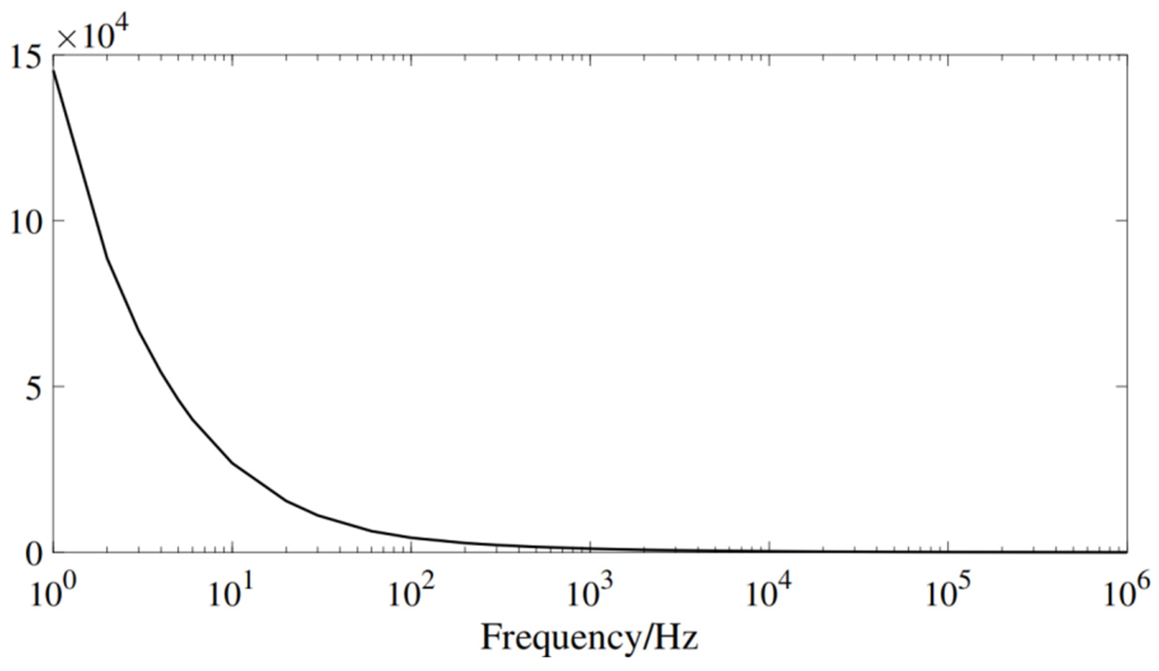
As can be seen from Equations (7) and (8), the values of $K_i$ and $K_o$ will change with frequency, because parameters such as $Z_{\mathrm{c}}$, $Z_{\mathrm{c}\mathrm{o}\mathrm{n}}$, $Z_{\mathrm{a}\mathrm{c}}$, and $s{L}_{\mathrm{D}\mathrm{C}}$ all vary with frequency. 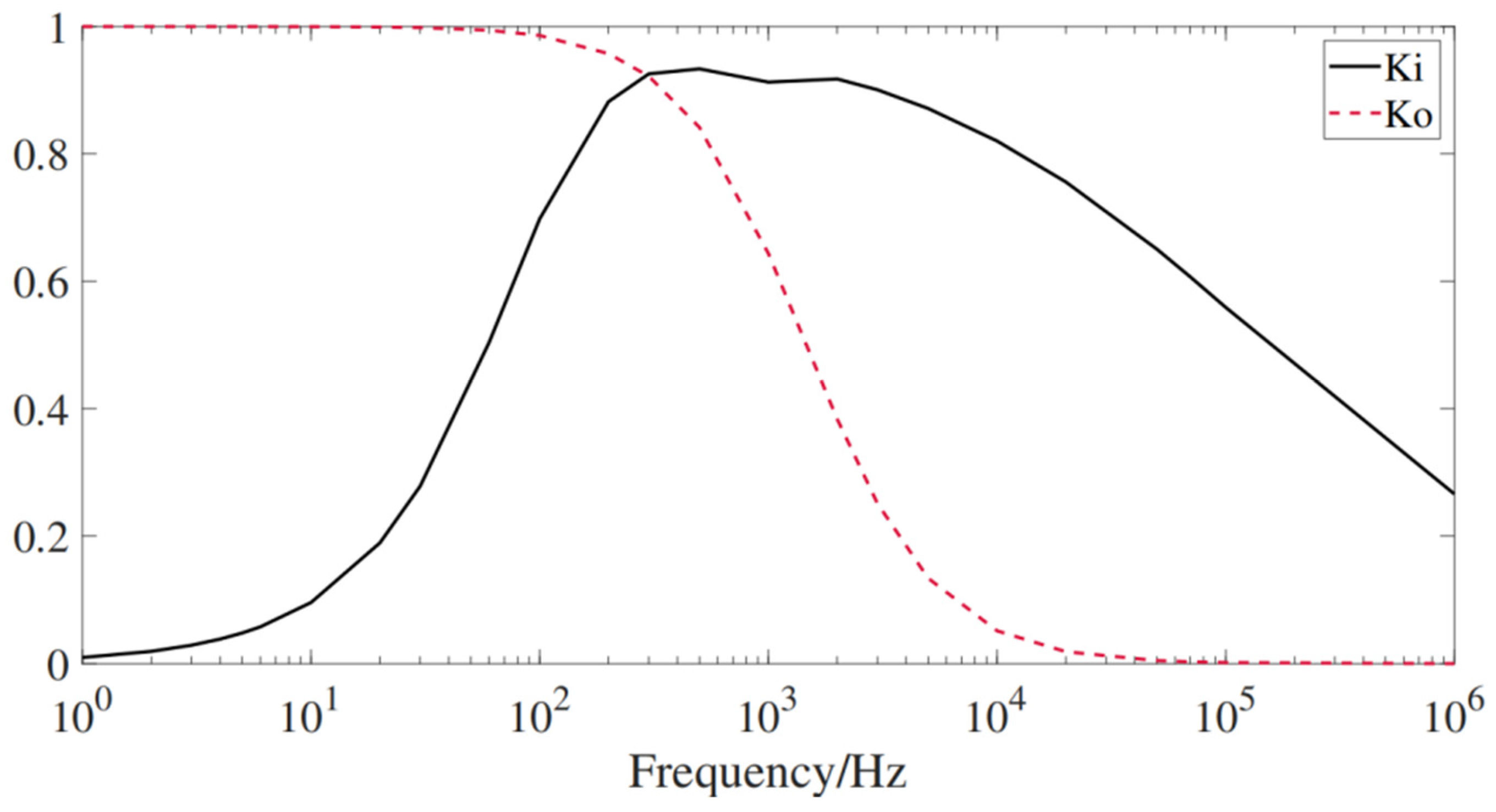Taking the cable in a DC grid as an example, the amplitude of the wave impedance $Z_{\mathrm{c}}$ at different frequencies can be obtained, as shown in Figure 3. The frequency response, in terms of the magnitude of the transfer function for the internal and external faults, was then computed, as shown in Figure 4. It can be observed that in the case of an external fault, the voltage attenuates much more rapidly in the high-frequency region. From the perspective of the frequency domain, the fault travel waves caused by internal and external faults show obvious differences when passing through the current-limiting reactor because of the inhibition effect of the reactor on the high-frequency components of the travel wave. Current-limiting reactors have also become natural barriers for DC fault protection. The principle behind the proposal of highly selective protective measures is to incorporate this boundary characteristic.

2.2. CEEMDAN

Based on the aforementioned disparity in high-frequency impedance along the travel path during internal faults compared with external faults, it can be anticipated that the transient features of the high-frequency components of the DC fault voltage will vary between internal and external faults.

Before extracting transient features from the high-frequency component, the DC voltage traveling wave was decomposed into several single-frequency components. Improved Empirical Mode Decomposition (EMD) and Complete Ensemble Empirical Mode Decomposition with Adaptive Noise (CEEMDAN) were used in this study. This method adds multi-white noise to the signal being processed and calculates the average intrinsic mode function (IMF) by summing all the decomposition results after each EMD of the signal with white noise. The influence of noise was canceled by multiple superpositions and averaging. Once the first-order IMF component is calculated, white noise is included in the residual value. Subsequently, the average value of the next-order IMF component was computed using the same calculation procedure. This process was repeated until all the components were calculated by multiple iterations. Compared to EMD, CEEMDAN has a faster computing speed and more completely decomposed signals. Moreover, unnecessary low-frequency components were reduced, which contributed to the rapid analysis of the frequency characteristics of the traveling waves.

The DC voltage on the line side of $L_{\mathrm{D}\mathrm{C},ij}$, denoted as $U_{i,\mathrm{L}\mathrm{i}\mathrm{n}\mathrm{e}}$, undergoes decomposition into several IMFs, each characterized by a specific frequency, using the CEEMDAN method. The expression for $U_{i,\mathrm{L}\mathrm{i}\mathrm{n}\mathrm{e}}$ can be formulated as Equation (9):

$$U_{i,\mathrm{L}\mathrm{i}\mathrm{n}\mathrm{e}}=\sum _{k=1}^n{c}_k(t)+r_n(t)$$

(9)

where $c_k\left(t\right)$ is the order k of the IMF component and $r_n\left(t\right)$ is the remainder.

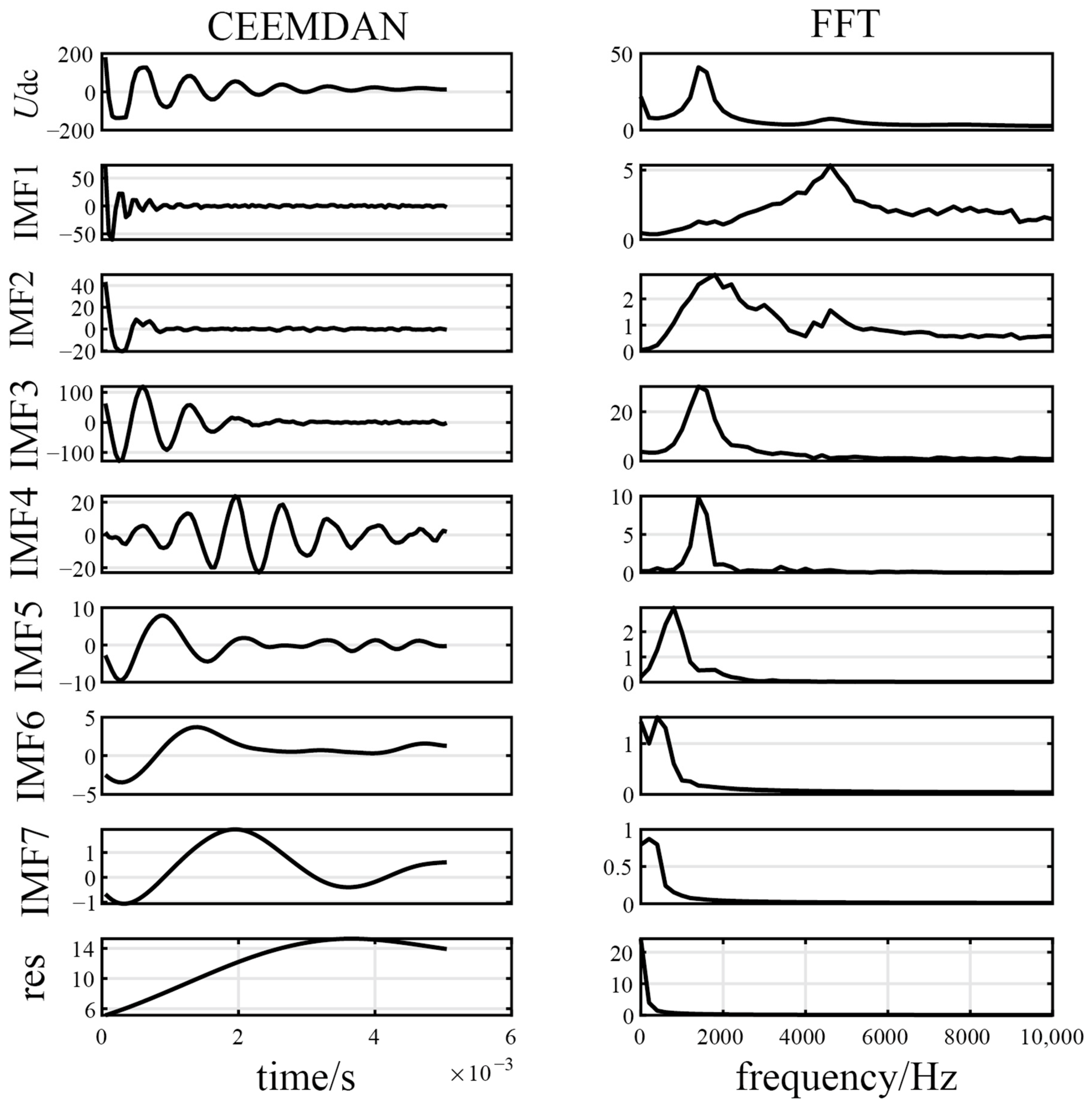
In the DC grid illustrated in Figure 1, when an internal DC grounding fault occurs at a distance of 30 km from the head end of Line₁₄, the voltage measured by relay R₁₄ is processed using the CEEDMAN method. The resultant outcome is presented in Figure 5. Simultaneously, the frequency spectrum of each signal was analyzed using a fast Fourier transform (FFT). IMF₁ contains the highest frequency component, and the frequency of the subsequent IMFs progressively decreases. The transient characteristics of the IMF are significantly influenced by the varying effects of the grounding resistance, CLR, and distribution parameters of the transmission line. These variations can significantly affect the behavior of high-frequency signals under different fault conditions. Consequently, the key features related to the most important information regarding the fault can be extracted from IMF₁.

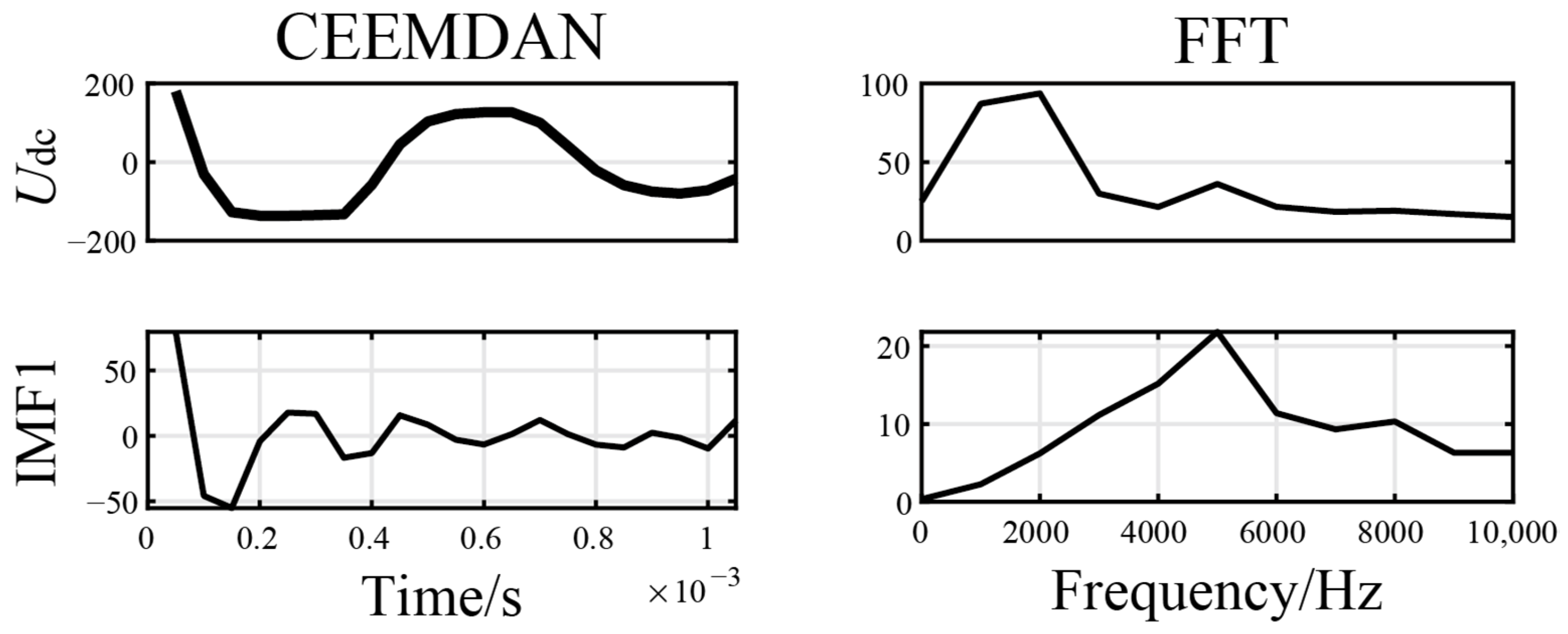
To improve the calculation speed and reduce the number of calculations, a fault identification criterion was set up to detect the wavefront of the traveling wave. Upon arrival of the fault voltage at the relay, the wavefront of the voltage traveling wave within milliseconds was decomposed by CEEMDAN for feature extraction. As illustrated in Figure 6, under fault conditions identical to those in Figure 5, only the first 1 ms of post-fault voltage information is analyzed through time–frequency analysis. By narrowing the time window to 1 ms—a duration sufficiently short to ensure rapid fault detection—IMF₁ retains the high-frequency characteristics of the DC voltage, as shown in Figure 6. This highlights the method’s capability to capture transient fault signatures within ultra-short intervals, thereby achieving an effective balance between speed and accuracy in fault diagnosis.

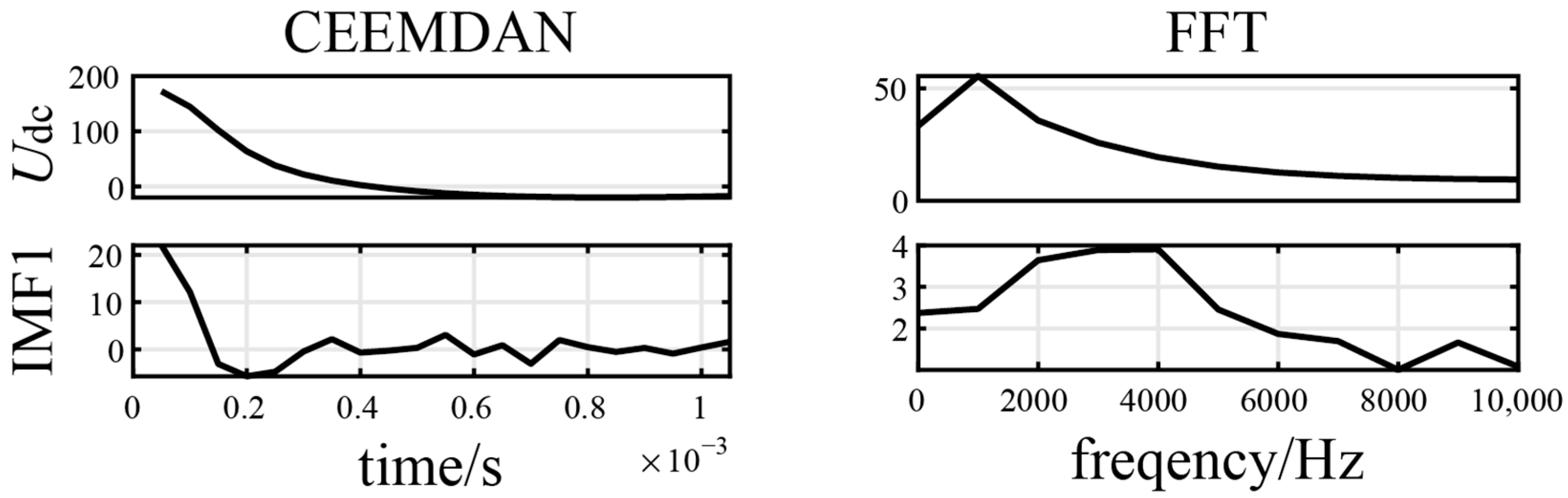
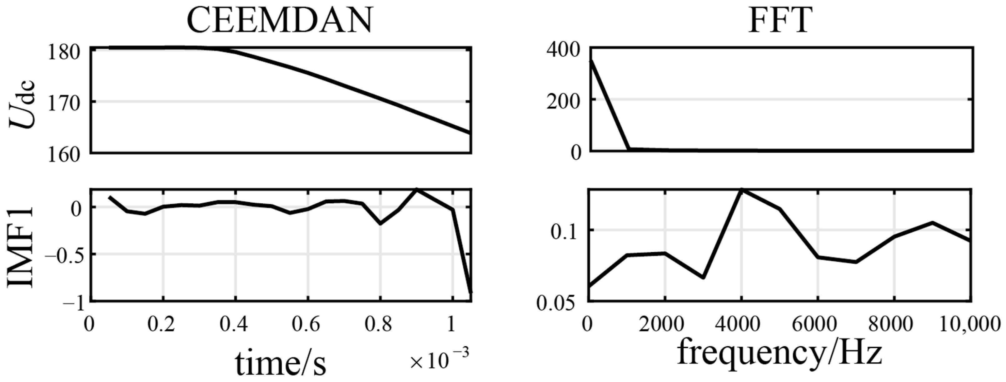
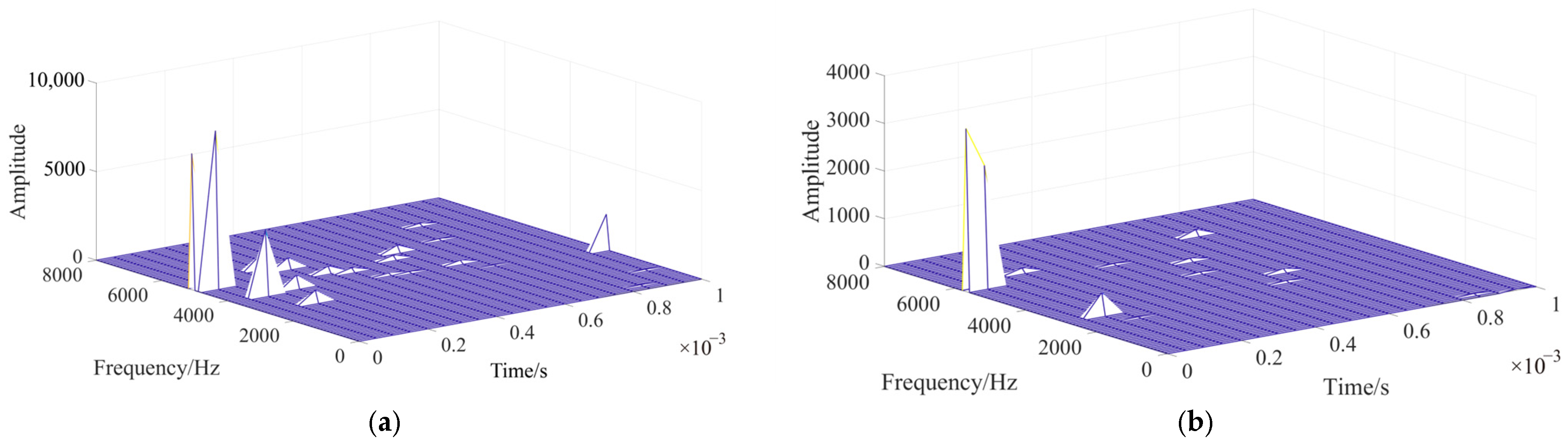
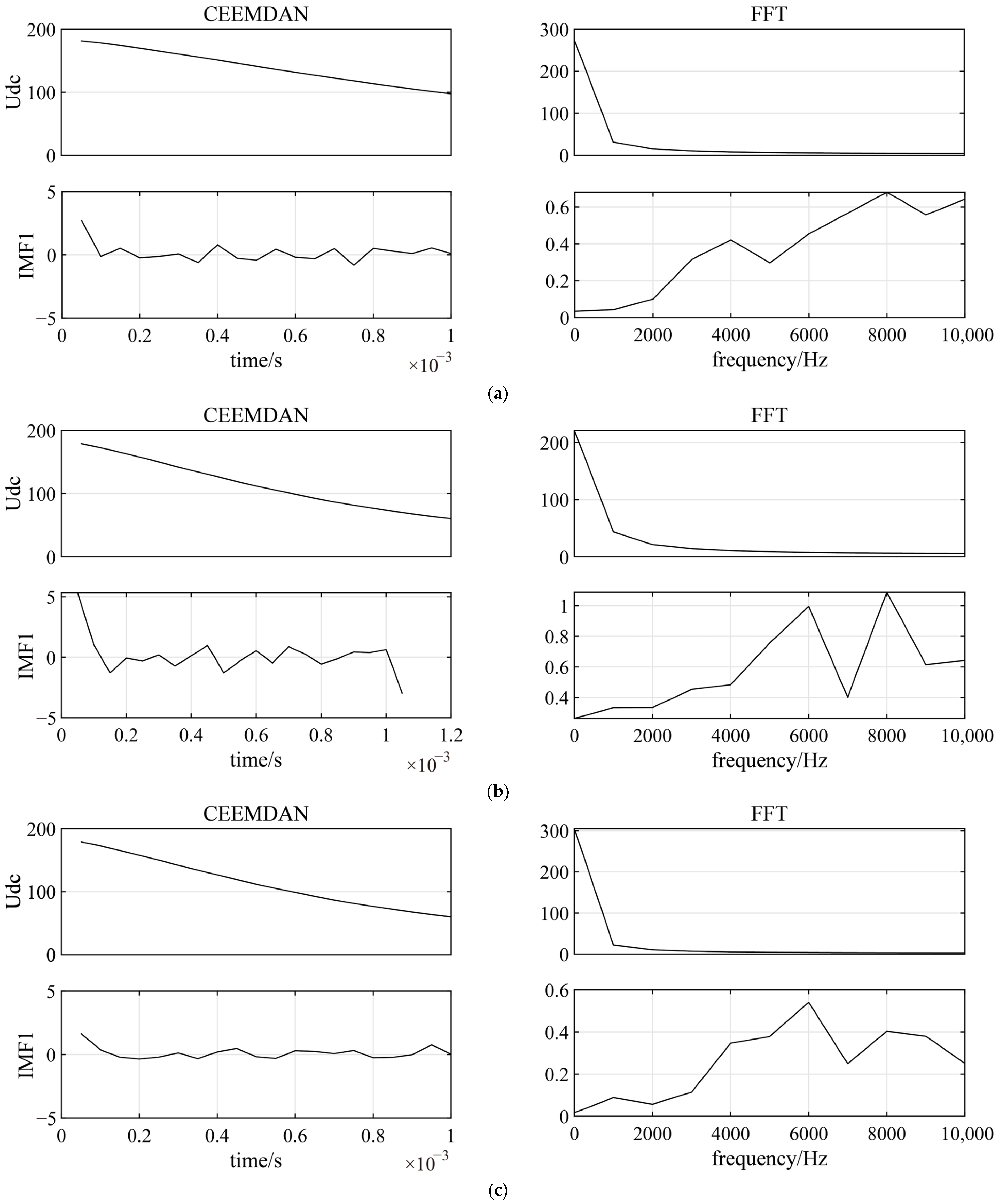
During fault identification, two specific types of faults pose significant challenges in differentiation: long-distance high-resistance faults and severe external faults. As illustrated in Figure 7, an internal high-resistance fault occurs at the end of Line₁₄ with a high grounding resistance. In contrast, Figure 8 depicts an external metallic grounding fault located beyond the reactor at the line terminal. Given the extensive propagation distance, the fault voltage experiences considerable attenuation and distortion before reaching the relay R₁₄. As a result, the original DC voltage waveforms presented in Figure 7 and Figure 8 demonstrate comparable rates of decline and similar variation trends in their time-domain profiles. This similarity renders traditional time-domain features, such as voltage amplitude decay, inadequate for reliable fault discrimination. However, the contents of the high-frequency components under internal high-resistance faults and external faults are different. Moreover, the derivative of IMF₁ at the moment the fault occurs under an external fault is decreased, from which adequate information about the fault can be extracted.

2.3. The Hilbert Transform

The Hilbert transform (HT) of the continuous signal x(t) is defined as Equation (10).

$$y(t)={\displaystyle \frac{1}{\pi }}P{\int }_{-\mathrm{\infty }}^{+\mathrm{\infty }}{\displaystyle \frac{x_{\delta }\left(\delta \right)}{t-\delta }}\mathrm{d}\delta$$

(10)

Signals $y\left(t\right)$ and $x\left(t\right)$ exhibit a complex relationship, facilitating the derivation of the analytical signal $z\left(t\right)$ through the subsequent procedure.

$$z(t)=x(t)+i\cdot y(t)=a(t)\cdot e^{i\theta (t)}$$

(11)

where $a\left(t\right)$ and $\theta \left(t\right)$ are the instantaneous amplitude and phase, respectively, which can be calculated as

$$a(t)=\sqrt{x^2\left(t\right)+y^2\left(t\right)},\theta =arctan{\displaystyle \frac{y\left(t\right)}{x\left(t\right)}}$$

(12)

The instantaneous frequency can be computed as

$$f(t)={\displaystyle \frac{1}{2\mathsf{\pi }}}{\displaystyle \frac{\mathrm{d}\theta \left(t\right)}{\mathrm{d}\left(t\right)}}$$

(13)

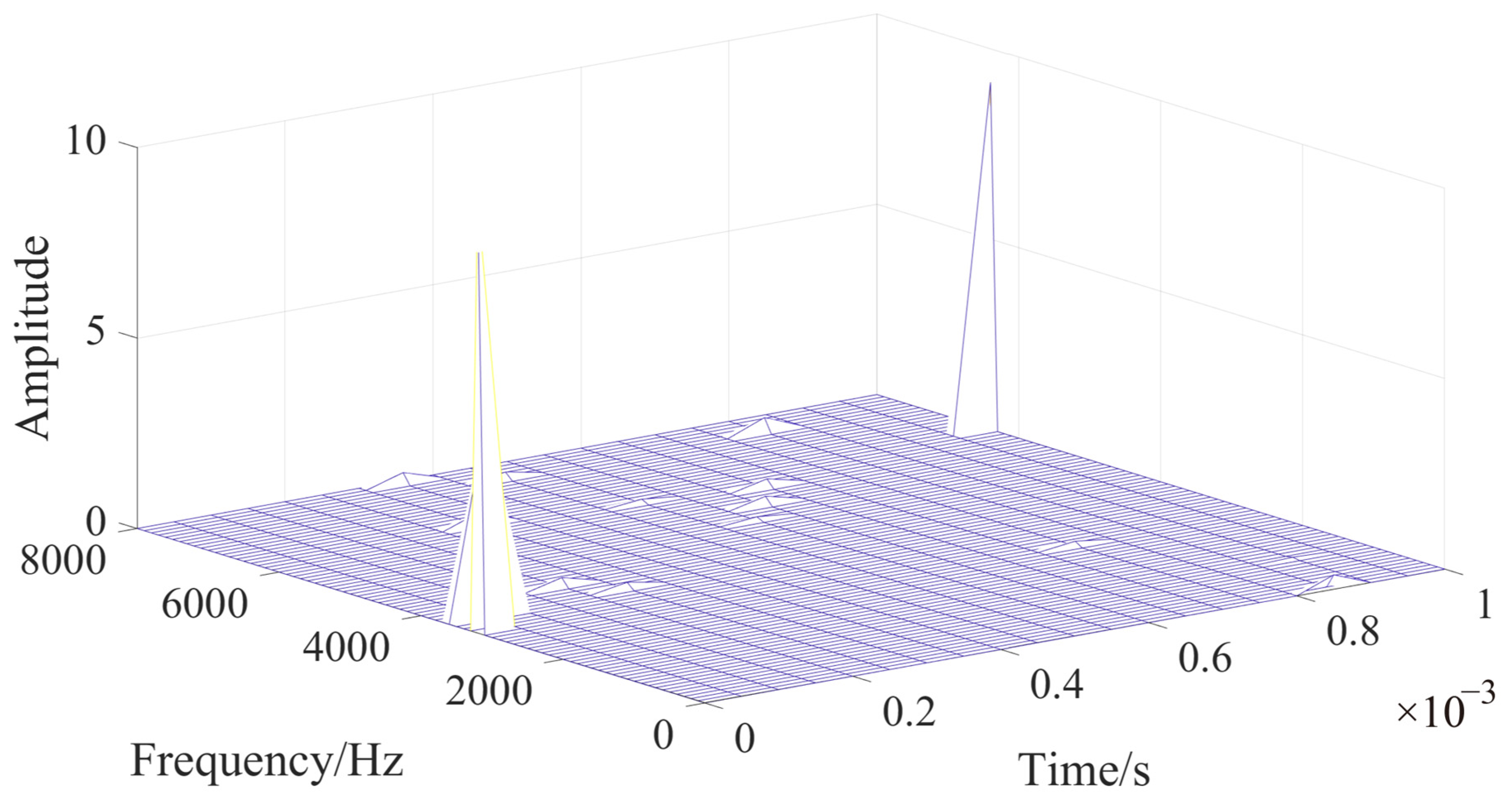
As shown in Figure 9, the Hilbert spectrum of IMF₁ (from the 1 ms time-window analysis in Figure 6) corresponds to an internal fault occurring on Line₁₄. The spectrum clearly illustrates the time-varying distribution of instantaneous frequencies and amplitudes under the specified fault condition. At 0 s, the moment the fault occurs, the instantaneous frequency and amplitude are at an extreme point because the voltage signal at the position of the traveling wave head decreases sharply at the moment of failure. As the voltage traveling wave propagates through the DC transmission lines, the wavefront attenuates gradually, whereas the steepness decreases. This change can be quantitatively characterized by the instantaneous frequency and amplitude of the high-frequency component. The extreme points in the Hilbert spectrum near 0 s are referred to as $f_0$ and $a_0$. Predictably, $f_0$ and $a_0$ change with changes in the fault position, grounding resistance, and inductance of the RLC.

3. The Proposed Fast Single-Ended Protection Scheme

By extracting the instantaneous high-frequency features ($f_0$, $a_0$) with the HHT, a selective fault detection approach is proposed. To avoid the disadvantages of the fault detection criterion with a threshold, a classification based on an SVM was employed in this study to distinguish between internal and external faults.

3.1. The SVM Classification

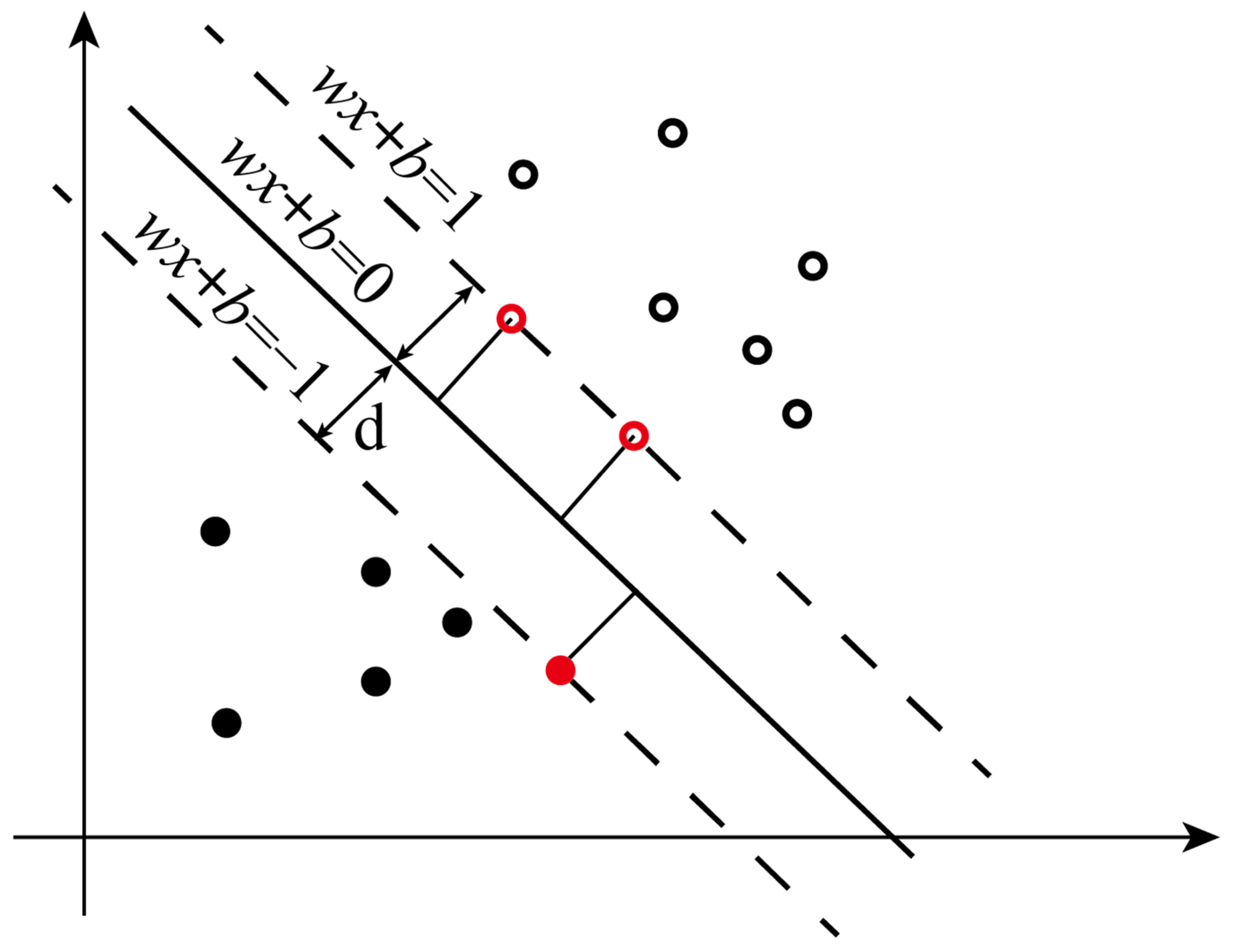
A support vector machine (SVM) is a binary classification model utilized in machine learning. It is adept at managing both linearly separable and linearly non-separable data, facilitating the construction of optimal decision boundaries within a high-dimensional space. As shown in Figure 10, a line can be drawn for a dataset to separate two sets of data points; such data are called linearly separable. The lines that separate the dataset are called the segmentation hyperplanes. The equation for this line in two dimensions is $y=ax+b$, and when generalized to n dimensions, it becomes a hyperplane equation $f\left(x\right)=w^{T}x+b$. The support vector (SV) refers to the collection of points closest to the hyperplane.

The purpose of an SVM is to find a hyperplane such that the sample is divided into two classes, and the space between the points and the hyperplane is the largest. Equation (14) represents a random hyperplane.

$$w^{T}x+b=0$$

(14)

The distance from each support vector to the hyperplane can be expressed as

$$d={\displaystyle \frac{|w^{T}x+b|}{\parallel w\parallel }}$$

(15)

In a binary classification problem, $y_i$ represents the label $x_i$, which has a value of 1 or −1. For any class $x_i$, $y\left(w^T+b\right)>0$. Therefore, $y\left(w^T+b\right)=|w^T+b|$.

The maximization of distance d can be expressed as an optimization problem in Equation (16).

$$\mathrm{m}\mathrm{a}\mathrm{x}2\times {\displaystyle \frac{y(w^{T}x+b)}{\parallel w\parallel }}$$

(16)

For ease of derivation, ||w||d is assumed to be 1. Thus, vector y (w^Tx + b) = 1. The optimization problem is given by Equation (17).

$$\mathrm{m}\mathrm{a}\mathrm{x}{\displaystyle \frac{2}{\parallel w\parallel }}$$

(17)

For calculation convenience, the formula is written as

$$\mathrm{m}\mathrm{i}\mathrm{n}{\displaystyle \frac{1}{2}}\parallel w{\parallel }^2\mathrm{s}.\mathrm{t}. y_i(w^T{x}_i+b)⩾1$$

(18)

3.2. Proposed Detection Method by HHT-SVM

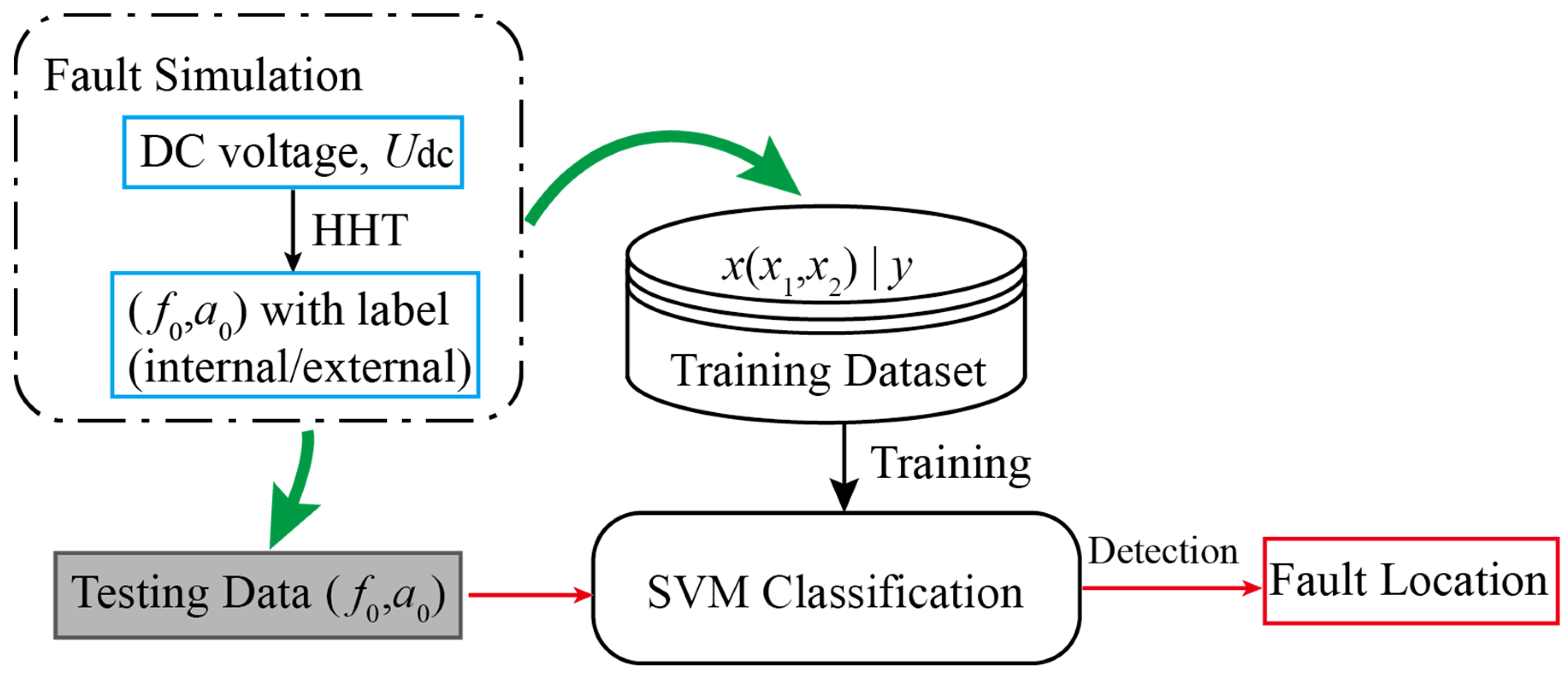
The analysis of high-frequency characteristics in fault voltage shows that the instantaneous frequency ($f_0$) and amplitude ($a_0$) of the DC voltage signal on the line side of CLR are crucial indicators for identifying internal versus external faults. The existence of current-limiting reactors at both ends of a DC line results in obvious changes in the high-frequency components $f_0$ and $a_0$ after fault voltage propagation. Thus, in a space constructed with the abscissa $f_0$ and ordinate $a_0$, the points of the “inside” and “outside” types are clustered in different regions. A fault detection method for DC fault classification was proposed by segmenting the space using an SVM.

As shown in Figure 11, this study utilized a large amount of data obtained from simulations of internal and exterior faults, which vary in terms of fault lengths and transition resistance. The purpose of these data was to train an SVM classification model. The remaining data were utilized to thoroughly assess the accuracy of the SVM classification.

3.3. The Protection Algorithm

3.3.1. Fault Identification Criterion

This technique uses local measurements of the DC current and voltage at one end of the DC line. To minimize the computational workload, the DC voltage drop criterion, represented by Equation (19), is first used to determine the presence of a DC fault in the DC grid. Subsequently, the alteration in the direction of the DC current signal is used to pinpoint the direction of the fault.

$$\mathrm{m}\mathrm{a}\mathrm{x}\left(\right|∆U_{i,\mathrm{L}\mathrm{i}\mathrm{n}\mathrm{e}\mathrm{p}}|,|∆U_{i,\mathrm{L}\mathrm{i}\mathrm{n}\mathrm{e}\mathrm{p}}\left|\right)>U_{\mathrm{r}\mathrm{e}\mathrm{q}}$$

(19)

The measured current flowed in a positive direction from the relay to the other terminal. Therefore, a forward fault was loaded in the positive direction of the fault current. The fault direction criterion was set as follows:

$${\displaystyle \frac{\mathrm{d}{I}_{\mathrm{d}\mathrm{c},ij}}{\mathrm{d}t}}>K_{\mathrm{d}\mathrm{i}}$$

(20)

where $K_{\mathrm{d}\mathrm{i}}$ was set to a value slightly greater than zero. If it is a forward fault, the data of the following 1 ms wave-front will be recorded for transient frequency feature extraction by HHT. The time-frequency analysis was conducted based on PyCharm 2024.1.7.

3.3.2. Flowchart of the Proposed DC Protection Strategy

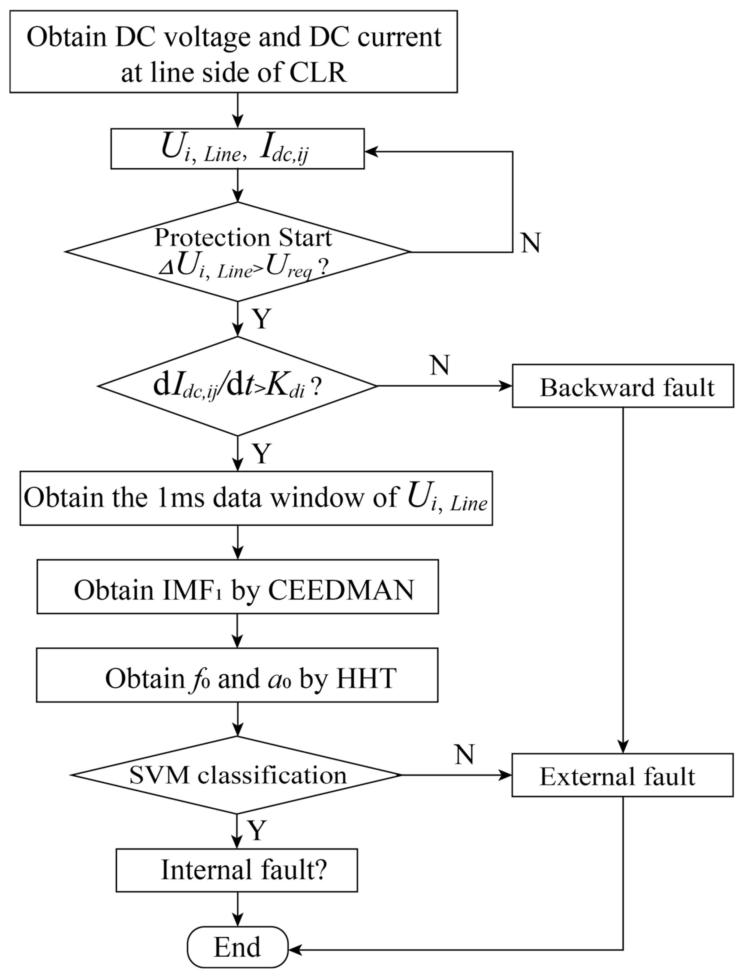
A flowchart of the proposed single-ended DC protection strategy is shown in Figure 12. The DC voltage and current were measured by the relay during the operation of the DC grid at the line side of the current-limiting reactor in series with the circuit breaker. Once the DC voltage drop reached the threshold value of the fault identification criterion, a DC-side fault was identified. The derivative of the fault current was then computed to determine the direction of the fault. A backward fault was noted as an external fault. For forward faults, the HHT-SVM-based fault detection starts to distinguish between internal and external faults. The 1 ms data at the front of the voltage traveling wave were recorded for feature extraction.

4. Simulation Verification

As shown in Figure 1, a ±200 kV four-terminal symmetric monopole HVDC grid was built in the PSCAD/EMTDC 4.6.2 software environment. VSC stations employ widely recognized modular multilevel converters (MMCs). The cables that connect them use a frequency-dependent (phase) line model.

Table 1. Converter and grid parameters.

	Conv. 1	Conv. 2–4
Rated capacity [MVA]	360	120
Rated DC voltage [kV]	±200	±200
Rated AC voltage [kV]	220	220
Operation Mode Setpoints	Constant DC voltage control ±200 [kV]	Constant active power control 100 [MW]

presents the parameters of the primary system.

The DC circuit breakers (CB) were installed at both ends of each DC line. As shown in 1, taking CB₁₄, the circuit breaker at the head end of Line₁₄, as an example, obvious voltage and current changes will be observed in the circuit breaker when faults occur in the transmission line of the DC power network, such as f₁–f₅. To limit the fault area, only when the internal fault f₁ is accurately identified will a trigger signal be generated to cut off CB₁₄. The same is true for other circuit breakers.

4.1. Influence Factors on the Transient Features

The influences of the CLR, grounding resistance, and distributed parameters of the cable on the high-frequency components of the traveling waves are different. The different effects of these parameters coincide transparently with variations in instantaneous frequency and amplitude. Simulations were performed to study the relationship between the fault parameters and transient frequency characteristics.

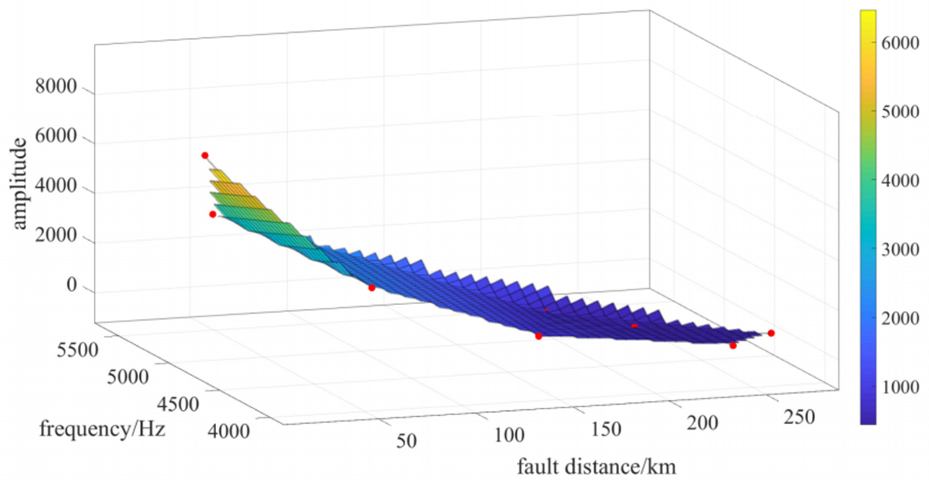
4.1.1. Influence of Fault Distance

The fault distance l changes from 10 to 270 km, the grounding resistance $R_{\mathrm{g}}$ is 0, and CLR $L_{\mathrm{D}\mathrm{C}}$ is 100 mH. The Hilbert spectrum of IMF₁ of the DC voltage under faults at different distances is shown in Figure 13.

The initial instantaneous frequency $f_0$ and amplitude $a_0$ demonstrated a clear decreasing trend as the fault distance increased. This relationship is illustrated in Figure 14. The instantaneous frequency and amplitude were quite high, with the fault located 10 km from the monitoring point. $f_0$ and $a_0$ decreased simultaneously owing to the effects of distributed resistance and inductance. When l changes from 10 to 270 km, $f_0$ and $a_0$ vary over a wide range.

4.1.2. Influence of Grounding Resistance

Simulations were performed with the grounding resistance $R_{\mathrm{g}}$ changed from 0 Ω to 100 Ω, while the fault distance l remained at 30 km and the CLR $L_{\mathrm{D}\mathrm{C}}$ remained at 100 mH. The instantaneous frequencies and amplitudes for the different transition resistances are shown in Figure 15. It is evident that, as the transition resistance increases, the transient amplitude decreases rapidly, whereas the instantaneous frequency varies less.

4.1.3. Influence of the CLR

As mentioned above, when the voltage surge wave generated by an external fault travels through the current-limiting reactor at the end of the terminal, the high-frequency components are filtered out by the reactor. This boundary characteristic is the principle behind frequency-domain fault protection in a DC grid. The Hilbert spectrum of the voltage under the fault at Bus 4 is shown in Figure 16. It is evident that there are very few high-frequency components measured by the relay at the head terminal of Line₃₄. A comparison of high-frequency components with reactance changes is shown in Figure 17. When the reactance of $L_{\mathrm{D}\mathrm{C}}$ is reduced, the voltage change rate increases. The instantaneous frequency at the time of fault occurrence also increased.

4.2. Fault Detection

The reliability of the proposed fault protection scheme was verified by simulation experiments in this section. Line₁₄ was set as the protected line. The operation of the corresponding circuit breaker was then determined through fault identification. According to the fault protection scheme process shown in Figure 12, first determine whether a DC side fault occurs and whether it is a forward fault based on the locally measured voltage and current signals, and then further distinguish whether it is an internal fault by an SVM.

Before validating the fault-diagnosis scheme, an SVM was trained and tested. A multitude of simulations were conducted within the PSCAD model. The fault conditions for the simulations are listed in

Table 2. Simulation data for SVM training and testing.

Training Dataset
Fault distance from Bus 3	10 60 90 150 210 270 300 340 380 420
Fault resistance [Ω]	0 10 30 60 90 100 200
Testing dataset
Fault distance from Bus 3	30 90 120 180 240 320 360 400
Fault resistance [Ω]	0 10 30 60 90 100 200

. A portion of the simulation results was used for training, and another portion was used for testing.

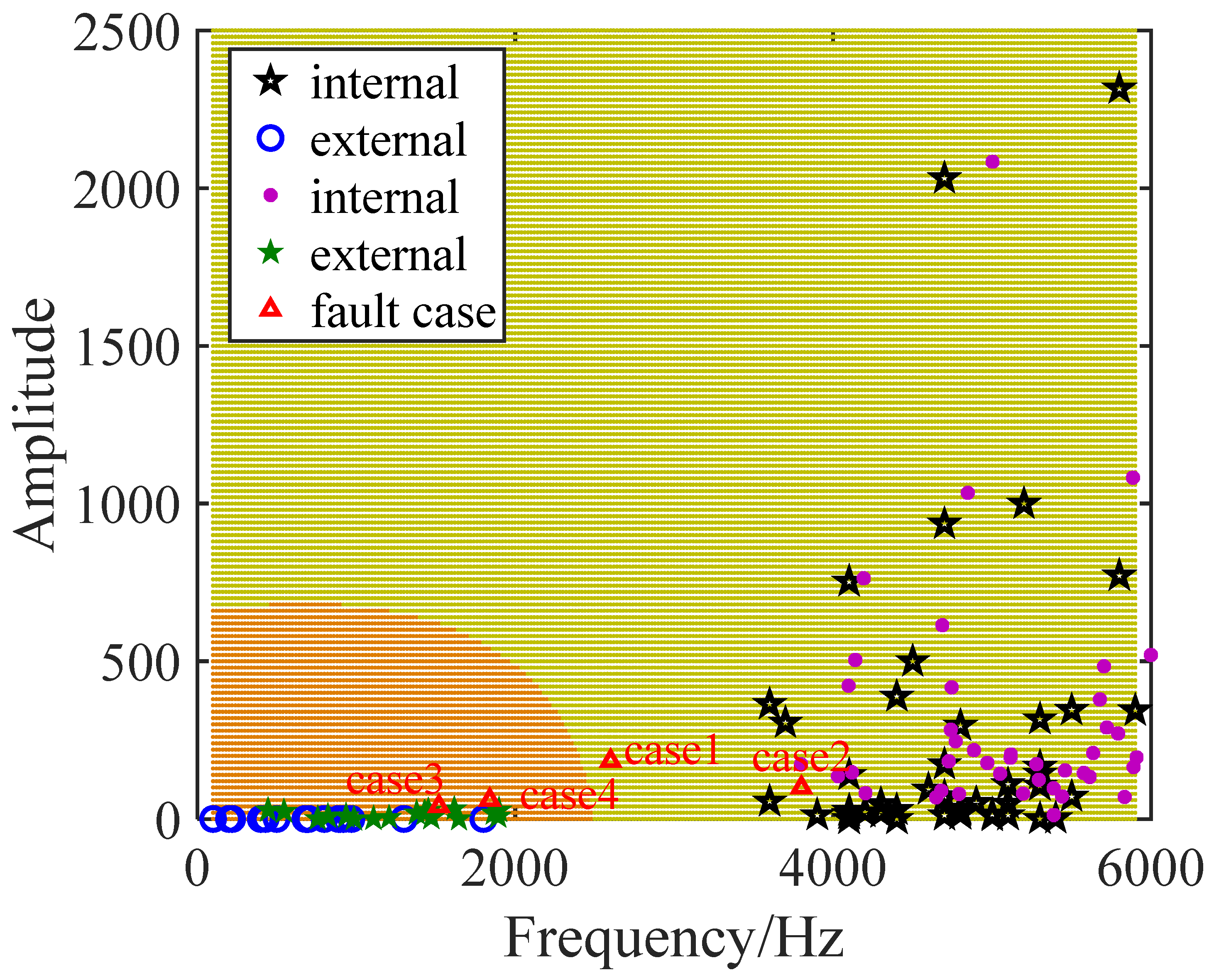
The training and testing results of the SVM are shown in Figure 18. In a two-dimensional space composed of instantaneous frequency and amplitude, the black star in the training point represents the internal problem, while the blue circle represents the external defect. The SVM was trained to divide this space into two parts: the orange external fault region and the yellow internal fault region. Fault detection based on an SVM using test data obtained from simulations verified the classification accuracy. In Figure 18, the purple dots indicate internal faults and the corresponding green pentagrams represent external faults. The test results match the fault positions in the simulations. To evaluate the performance of the SVM, indicators such as accuracy, precision, recall, and F1 score were selected to evaluate the classification results under different fault scenarios. As the results show in

Table 3. The classification results across different fault scenarios.

Fault Scenario	Accuracy	Precision	Recall	F1-Score
Internal High-Resistance Faults	98.3%	97.5%	98.1%	97.9%
Internal Low-Resistance Faults	99.2%	99.1%	99.5%	98.6%
Internal Remote Faults	96.8%	97.2%	97.1%	96.4%
External Severe Ground Faults	98.1%	97.9%	97.4%	97.5%
External High-Resistance Faults	98.6%	99.5%	97.7%	98.3%
External Remote Faults	96.8%	95.9%	97.6%	96.7%

, the SVM demonstrates consistently outstanding performance in terms of classification accuracy for all tested fault scenarios.

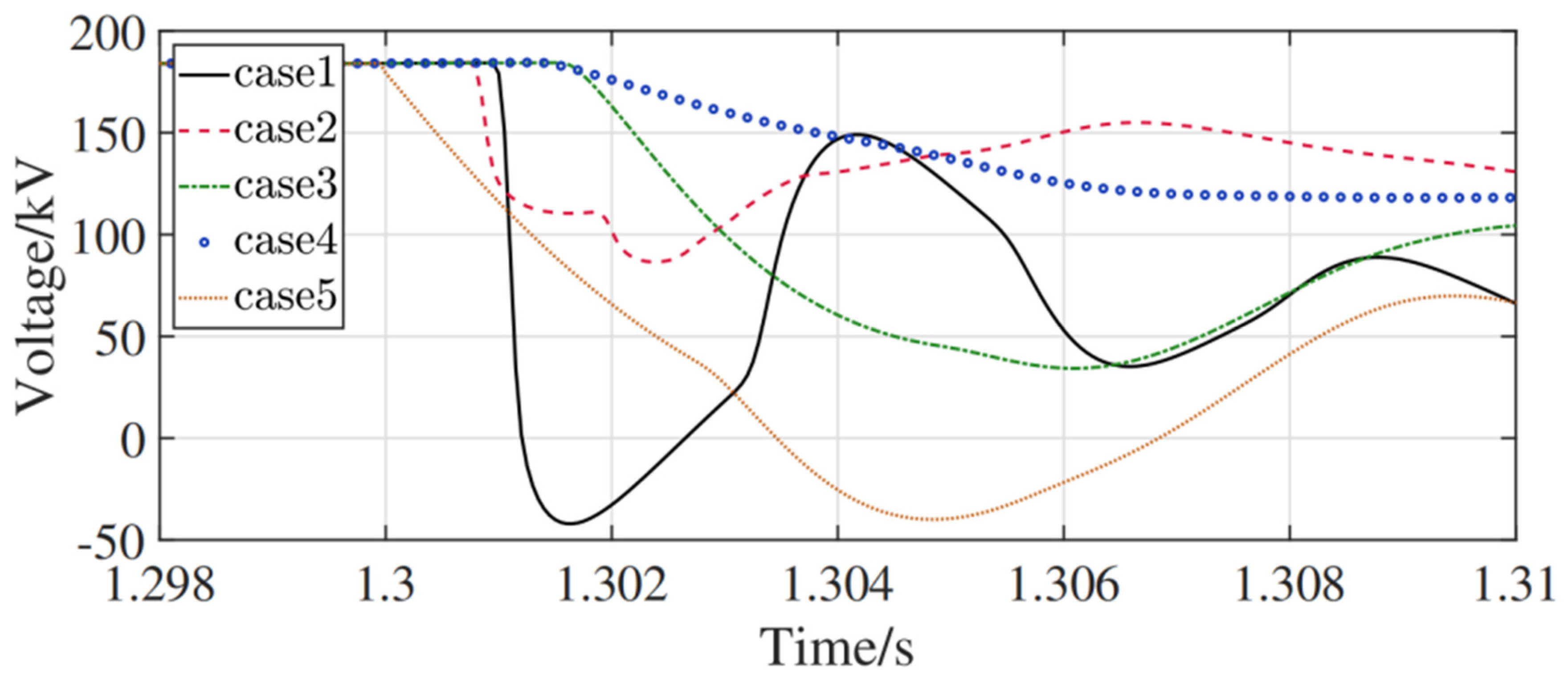
Simulations were conducted to verify the protection scheme proposed in this study. Based on the built DC grid simulation model, Line₁₄ is designated as the protected line. By single-ended protection requirements, measurements are conducted by relay R₁₄ adjacent to circuit breaker CB14 at the line’s head end, with fault types identified via local signals. Although faults occur simultaneously, their arrival times at R14 differ due to varying distances. The specific fault conditions are as follows: Case 1 is an internal pole-to-pole fault on Line 14, located 140 km from R14; Case 2 is a pole-to-ground fault on Line 14 at 160 km from R14 with a grounding resistance of 60 Ω; Case 3 is a pole-to-ground fault on Line 45 at 300 km from R14 (external to Line 14) with a grounding resistance of 30 Ω; Case 4 is a pole-to-ground fault on Bus 4 (external to Line 14) with a metallic ground; and Case 5 is a pole-to-pole fault on Bus 2 (external to Line 14). The latter three cases (Cases 3–5) are categorized as external faults with respect to Line 14.

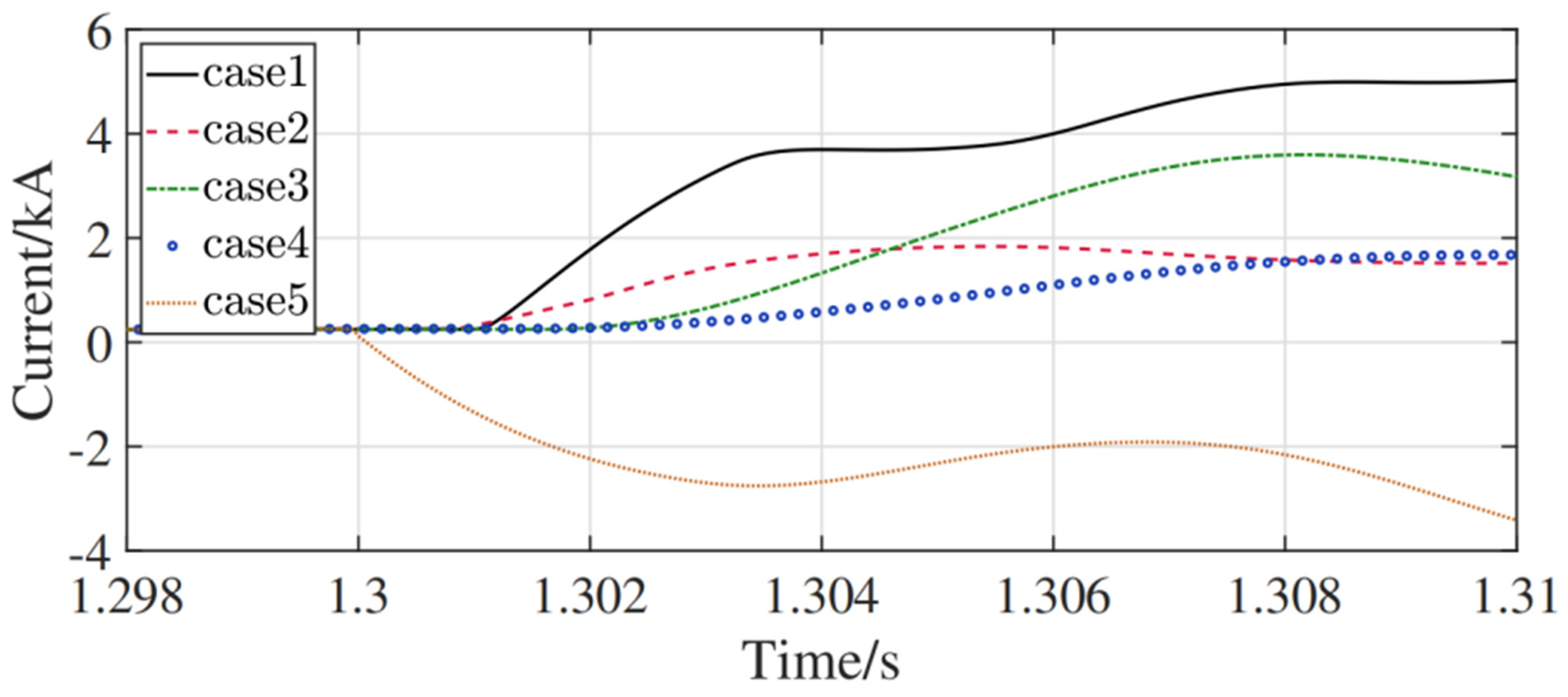
Figure 19 shows the voltage variation after a fault. In every condition, the DC voltage decreased when the fault appeared. Therefore, it is determined that a DC-side fault has occurred, and the DC-side fault protection is activated. As shown in Figure 20, the variation in the fault current was used to determine the direction of the fault. In Cases 1 to 4, the fault current variation rate is positive, which indicates straightforward faults. Case 5 represents a negative fault current variation rate, which is determined as a backward fault, that is, an external fault. Intercepting voltage waveform data 1 ms after Case 1–Case 4 fault occurrence, SVM fault identification was applied after extracting the fault characteristics of high-frequency components with HHT. As shown in Figure 18, Cases 1 and 2 were determined to be internal faults, whereas Cases 3 and 4 were determined to be external faults. The results prove the reliability of the fault-protection solution.

5. Conclusions

This study explores the transient characteristics of the high-frequency component of the voltage traveling wave under DC faults. Due to the characteristics of the current-limiting reactor of the faulty circuit and the distribution parameters of the line varying with frequency, the internal and external fault voltages show significant characteristic differences in the high-frequency region. The time–frequency characteristics of the high-frequency components of the fault voltage are analyzed through HHT, and the instantaneous frequency and instantaneous amplitude of the high-frequency components of the voltage traveling wave are extracted as the characteristic parameters for fault identification. The results show that the instantaneous frequency and amplitude decrease rapidly with an increase in the fault distance, and high transition resistance mainly reduces the instantaneous amplitude. Due to the filtering effect of the current-limiting reactor, the transient frequency of external faults is significantly lower than that of internal faults.

This study utilizes the transient high-frequency characteristics of voltage traveling waves during faults and proposes a novel single-ended protection scheme for DC power grids. Through Hilbert–Huang transform (HHT) analysis, the instantaneous frequencies and amplitudes of the high-frequency components excited by faults were extracted as discriminative features, revealing the significant mode differences between internal and external faults. The proposed classification method based on a support vector machine (SVM) effectively eliminates the need for manually setting protection thresholds, showing fast response, high selectivity and reliable performance, especially with significant advantages in challenging fault scenarios such as high resistance and long distance.

Simulation results in PSCAD validate the feasibility of the approach, confirming its ability to accurately classify faults under varying system conditions. However, this method mainly relies on simulation data for simulation and data analysis. In practical applications, it may be affected by factors such as electromagnetic interference, cable aging, and measurement noise. Furthermore, the model’s simplification treatments such as idealizing cable characteristics and ignoring environmental influences may lead to a decrease in the effectiveness of the support vector machine when the real fault characteristics differ significantly from the simulation. To address these limitations, future research should focus on conducting field tests in actual high-voltage direct current power grids and collecting real data to enhance the practicability of the methods. At the same time, develop more accurate physical models to better cope with actual complex scenarios.