Abstract
Accurate predictions of the temperature of battery energy storage systems (BESSs) are crucial for ensuring their efficient and safe operation. Effectively addressing both the long-term historical periodic features embedded within long look-back windows and the nuanced short-term trends indicated by shorter windows are key factors in enhancing prediction accuracy. In this paper, we propose a BESS temperature prediction model based on a convolutional neural network (CNN), patch embedding, and the Kolmogorov–Arnold network (KAN). Firstly, a CNN block was established to extract multi-scale periodic temporal features from data embedded in long look-back windows and capture the multi-scale correlations among various monitored variables. Subsequently, a patch-embedding mechanism was introduced, endowing the model with the ability to extract local temporal features from segments within the long historical look-back windows. Next, a transformer encoder block was employed to encode the output from the patch-embedding stage. Finally, the KAN model was applied to extract key predictive information from the complex features generated by the aforementioned components, ultimately predicting BESS temperature. Experiments conducted on two real-world residential BESS datasets demonstrate that the proposed model achieved superior prediction accuracy compared to models such as Informer and iTransformer across temperature prediction tasks with various horizon lengths. When extending the prediction horizon from 24 h to 72 h, the root mean square error (RMSE) of the proposed model in relation to the two datasets degraded by only 11.93% and 19.71%, respectively, demonstrating high prediction stability. Furthermore, ablation studies validated the positive contribution of each component within the proposed architecture to performance enhancement.
1. Introduction
With the ongoing transformation of energy structures, the importance of battery energy storage systems (BESSs) is growing significantly [1,2]. Owing to advantages such as their high energy density and rapid response speed, lithium-ion batteries have emerged as the dominant technology for electrochemical energy storage [3]. However, the performance and state of health (SOH) of these batteries are significantly influenced by thermal effects during operation [4]. Furthermore, sustained exposure to high temperatures can potentially trigger thermal runaway events, posing serious safety risks to both personnel and equipment [5].
Relying solely on passive temperature monitoring and reactive thermal management strategies is often insufficient to address unforeseen operational conditions or emergencies. Accurate prediction of BESS temperature plays a crucial role in enhancing thermal management and operational safety. Such predictive capacity provides critical inputs that help battery management systems (BMSs) implement proactive thermal control strategies, optimizing operational performance [6,7]. Additionally, it facilitates early detection of potential thermal anomalies, enabling timely interventions to prevent safety-critical events [8,9].
The current research on BESS temperature prediction primarily falls into three categories: physics-based modeling methods, data-driven approaches, and hybrid-driven methods. Physics-based modeling methods offer strong interpretability and contribute to revealing the intrinsic heat generation mechanisms within BESSs [10,11]. Hybrid-driven methods typically leverage physical models to provide prior knowledge or constraints, while data-driven models are employed for residual correction, parameter identification, or modeling aspects that are difficult to capture with physical models. This synergy can enhance the accuracy of physical models and improve the interpretability of data-driven models [4,11]. However, methods involving physical models often require complex modeling and are subject to significant challenges in accurately acquiring necessary parameters and numerous limitations in practical applications.
Although physics-based modeling methods and hybrid-driven methods demonstrate potential, purely data-driven approaches are often favored for their adaptability and ability to learn directly from operational data, especially when detailed physical parameters are difficult to obtain [9]. Wang et al. [12] applied backpropagation neural networks (BP-NNs), radial basis function neural networks (RBF-NNs), and elman neural networks (Elman-NNs) to establish temperature prediction models for lithium-ion batteries under conditions involving metal foam and forced-air cooling. Their study demonstrated the feasibility of applying neural network techniques to the domain of temperature prediction.
The core of BESS temperature prediction involves time series forecasting. Jiang et al. [13] proposed a joint prediction method for predicting the maximum and minimum temperatures of a BESS based on an elitist genetic algorithm (EGA) and a bidirectional long short-term memory (BiLSTM) network. By optimizing the time series segmentation strategy and introducing an improved bidirectional loss function, this approach achieved superior prediction accuracy compared to standard LSTM and light gradient boosting machine (LightGBM) models. Recognizing the spatio-temporal nature of temperature data, Zhao et al. [14] integrated the spatial feature extraction capabilities of a convolutional neural network (CNN) with the temporal modeling advantages of LSTM networks, proposing a temperature prediction method for lithium-ion batteries based on a hybrid CNN-LSTM neural network. Using this method, they successfully predicted temperatures for various battery types. The success of the aforementioned studies provides a strong foundation and valuable insights for utilizing data-driven methods to assist in the thermal management of BESSs.
By accounting for the critical role of accurately capturing long-range dependencies in time series analysis, models based on attention mechanisms (AMs) have demonstrated exceptional capabilities and achieved significant success [15]. Consequently, various attention-based models have also been widely applied in predicting battery remaining useful life (RUL), SOH, and temperature [16,17,18,19]. Li et al. [20] proposed a method for lithium-ion battery surface temperature prediction based on empirical mode decomposition (EMD) and the Informer model. In this approach, the authors used EMD to decompose temperature data into intrinsic mode functions (IMFs), reconstructed the IMF components based on the Pearson correlation coefficient, and finally combined these reconstructed components with voltage and current data, feeding them into multiple sub-models to realize high-precision temperature prediction. Qi et al. [21] utilized EMD to decompose original temperature data into different components, subsequently employing an LSTM network augmented by an AM to learn long-term dependencies within the features. Ultimately applied to the temperature prediction of electric vehicle (EV) power batteries, experiments conducted under various operating conditions validated the method’s ability to handle high-frequency non-stationary noise. Hong et al. [22] presented a novel multi-forward-step prediction technique based on a spiral self-attention neural network (SS-ANN) for predicting battery temperature, combining the self-attention mechanism (SAM) with gated recurrent units (GRUs), achieving substantial performance improvements compared to those yielded by conventional LSTM models. The success of these studies underscores the importance of introducing attention mechanisms into the domain of BESS temperature prediction.
However, the monitoring data of BESSs operating in non-laboratory environments (e.g., EV power batteries, residential BESSs, and battery energy storage power stations) are influenced by user habits and routine dispatch commands. The temperature profiles of these BESSs often exhibit pronounced local fluctuations superimposed on underlying periodic characteristics. While attention-based models excel at capturing dependencies, proactively and effectively addressing both the long-term historical periodic features embedded within long look-back windows and the nuanced short-term trends indicated by shorter windows remains a crucial factor in enhancing prediction accuracy. Furthermore, accurately extracting key predictive information from complex features is also pivotal for improving temperature prediction precision.
To predict BESS temperature and address the multifaceted challenges previously discussed, we propose a customized CNN–Patch–Transformer model that utilizes a Kolmogorov–Arnold Network (KAN) for feature mapping. A comparison of the main features of this model with the aforementioned existing approaches is presented in Table 1. The CNN–Patch–Transformer model was designed as follows: Firstly, a CNN block was established to extract multi-scale temporal periodic features and multi-scale correlations among data points embedded within long look-back windows. This allows for the capture of global patterns in time series data and the interdependencies among monitored variables. Subsequently, to capture fine-grained local dynamics, a patch-embedding mechanism and a transformer encoder were introduced. This endows the model with the ability to extract local temporal features from segments within historical long look-back windows, enabling it to perceive subtle local variations in the time series. Finally, the KAN model was applied, leveraging the strong fitting capabilities of B-spline functions, to enhance the model’s ability to extract key predictive information from the complex, feature-rich data representations generated by the preceding components.

Table 1.
Comparison of main features of various methods.
2. Problem Definition
For the BESS composed of multiple battery modules, predicting the maximum and minimum temperatures of the entire BESS provides comprehensive reference information for decision-makers. Consequently, the temperature prediction task addressed in this study is fundamentally a multivariate time series forecasting problem with covariates, involving two target variables. When the length of the look-back window is L, the time series window for the maximum and minimum temperatures is defined as follows:
where represents the maximum and minimum temperature values at timestamp t.
Given Nz covariates, the covariate input window is defined as follows:
where denotes the covariate data at timestamp t.
The BESS temperature prediction problem can be formulated as follows: given the historical data X and covariate data Z within the look-back window, predict the maximum and minimum temperature data for the next T future time steps. This task can be represented by the following equation:
where represents the predicted output corresponding to the ground truth ; denotes the network model, with θ representing the model’s parameters; indicates the concatenation of X and Z along the first dimension; represents the concatenated look-back window; and N = Nz + 2.
The objective of this paper is to optimize the parameters θ of the neural network model using the gradient descent method, such that the predicted output closely approximates the ground truth . In this process, this paper employs the mean squared error (MSE) function as the loss function during the gradient descent procedure, which is calculated as follows:
where represents the predicted value of the i-th variable at time t, and represents the label value of the i-th variable at time t.
3. CNN–Patch–Transformer Model
To address the unique challenges presented by BESS temperature data, we introduce a customized CNN–Patch–Transformer model. Figure 1 illustrates the overall architecture of the CNN–Patch–Transformer model, wherein the CNN block is employed to extract multi-scale periodic temporal features and inter-variable multi-scale correlations from time series data embedded in long look-back windows. This design enables the model to address the daily periodicity inherent in BESS temperature data and integrate correlations among monitored variables at different scales, thereby enhancing temperature prediction accuracy. The patch-embedding mechanism and its corresponding encoder are utilized to extract local temporal features from long historical look-back windows, allowing the model to process subtle local fluctuations in temperature data. The KAN model then functions as a powerful decoder, mapping these complex, multifaceted features to accurate predictions. The operational mechanism of each module depicted in the figure will be described in detail in this section.
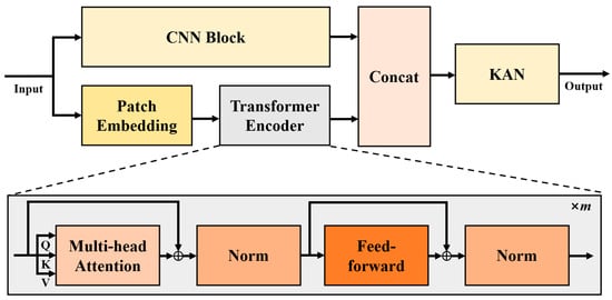
Figure 1.
Overall architecture of the CNN–Patch–Transformer model.
3.1. CNN Block
To extract multi-scale periodic features within long look-back windows, we designed a CNN-based feature extraction module. Its specific operational mechanism is detailed in the pseudocode presented below (Algorithm 1).
Within the CNN block, we first downsampled the look-back window data Nc times to obtain Nc sub-windows with varying sampling frequencies. Subsequently, operations were performed independently on each sub-window. Specifically, we performed N convolutions on the data within each sub-window. The processing method for each convolution is illustrated in Figure 2.
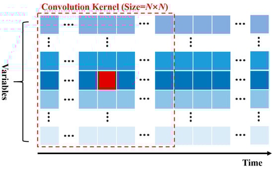
Figure 2.
Convolution method within the CNN block. In the figure, the identically colored blue squares represent the data of the same monitored variable at various time steps, and the red square represents the current convolution center.
| Algorithm 1: CNN Block | |
| 1 | |
| 2 | Downsample into Nc windows |
| 3 | for g = 1 to Nc do |
| 4 | |
| 5 | for n = 1 to N do |
| 6 | |
| 7 | |
| 8 | end for |
| 9 | |
| 10 | |
| 11 | Append hc to Hc |
| 12 | |
| 13 | return Hc |
According to Figure 2, during convolution, we first conceptually position the n-th time series at the center relative to all other series. Then, a convolutional kernel with dimensions of N × N is utilized for the convolution operation. The advantage of this approach is that it not only enables the convolutional kernel to fully extract concurrent correlated features between the variable being convolved and its surrounding variables but also the cross-temporal correlated features among the variables. It is noteworthy that, during convolution, both the beginning and end of the sequence are padded by replication. This ensures that the length of the sequence after convolution is equal to the length of the original sequence after the current downsampling operation.
After N convolutions have been performed on the data within a sub-window, the N sets of features obtained from these convolutions are concatenated and subsequently mapped to D dimensions using a linear projection. Once all sub-windows have undergone convolution, these Nc convolutional results are then concatenated to form the final extracted output of the CNN block.
3.2. Patch Embedding
To extract cross-temporal correlations from time series data within long look-back windows and accurately analyze the local temporal characteristics of the time series data, we employ the patch-embedding method [23]. Patch embedding processes each time series individually. When processing each time series, the sequence is first subjected to a patching operation [1], as illustrated in Figure 3:
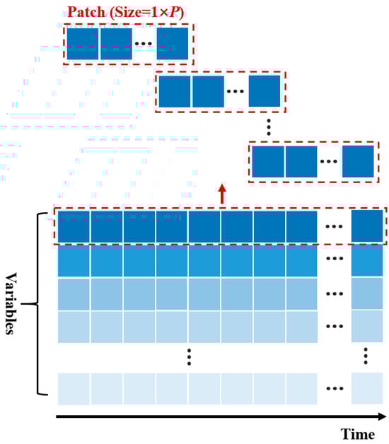
Figure 3.
Schematic diagram of the patching operation. In the figure, the identically colored blue squares represent the data of the same monitored variable at various time steps.
According to Figure 3, each sequence is divided into multiple patches with a length of P. During the division process, the degree of overlap between patches is controlled by the stride S. The patching process decomposes the sequence into sub-sequences. These sub-sequences for the n-th variable are collectively represented as . To ensure that each patch has an equal length, the end of the last patch is padded using replication.
After decomposing the sequence into patches, patch embedding is used to map the patches to embedded features through position embedding and a linear projection. The final embedding result is then represented as .
3.3. Transformer Encoder
As in most attention-based models, we also utilize a transformer encoder block to process the embedded features from patch embedding. The transformer encoder block employed in this study consists of a multi-head attention mechanism, normalization, and a feed-forward network (FFN) [24,25].
The multi-head attention mechanism first applies a linear mapping to the input . This projects the original embedding dimension D to dk to obtain learnable query, key, and value matrices. The query, key, and value matrices are then projected Nhead times to obtain Nhead individual attention heads. Finally, the outputs of these individual attention heads are concatenated and projected to produce the final computational result. In this process, the computation for a single attention head is performed as follows:
where Q, K, and V correspond to the query, key, and value matrices, respectively; dk = D/Nhead; and the scaling factor is used to prevent the dot products from becoming excessively large, which could lead to vanishing gradients in the softmax function.
The primary purpose of normalization is to stabilize the distribution of activation values during training, reduce internal covariate shift, accelerate model convergence, and potentially improve model performance. In this study, batch normalization was employed for the output of patch embedding.
We implement the FFN using linear layers. Finally, the dimensionality of the input remains unchanged after passing through one transformer encoder block.
3.4. KAN
After key predictive features have been extracted by the preceding modules, merely using a linear layer or a shallow multilayer perceptron (MLP) model may be insufficient for complex decoding tasks. Han et al. [26] experimentally demonstrated the effectiveness of KANs in multivariate time series forecasting tasks, also showing that replacing linear layers in other models with a KAN can yield superior benefits. In light of this, this paper employs a single-layer KAN to map the complex, multi-dimensional features extracted by the various preceding modules to temperature predictions.
Unlike traditional MLPs, which apply fixed activation functions neuron-wise, a KAN features learnable, univariate, spline-based activation functions on each network edge. This design is inspired by the Kolmogorov–Arnold representation theorem, which posits that any multivariate continuous function can be expressed as a finite composition of univariate functions and additions [27]. This composition can be formulated as
where xp is the p-th input feature, and and are both parameterized univariate spline functions, typically taken to be B-spline functions.
The capacity of a KAN to learn the optimal functional form for each connection is considered crucial for effectively transforming complex encoded information into precise temperature predictions. A KAN can be viewed as a special type of MLP, with its uniqueness stemming from the use of learnable B-spline functions as activation functions [28]. Leveraging the strong fitting capabilities of B-spline functions, KANs possess enhanced flexibility in modeling complex non-linear relationships, often leading to more accurate predictions than simpler decoders when mapping complex features to prediction results.
We did not employ a dedicated attention module in the decoding stage. Instead, we first concatenated the feature extraction results from the CNN block and the output of the transformer encoder processing the patch embedding into , where Ncat = Nc + Np. Subsequently, the concatenated result was flattened into . Then, the KAN model was used to map the flattened result to the prediction output . Finally, this output was truncated to obtain the required final prediction result .
4. Experiments and Analysis
4.1. Dataset Description
The two datasets employed in this study originate from residential BESSs located in Europe. Each BESS is composed of six battery sub-modules, and the chemical composition of the corresponding batteries is lithium iron phosphate (LFP). Henceforth, these datasets will be referred to as Dataset 1 and Dataset 2. Both datasets present an initial sampling frequency of 10 min and include monitored variables such as current, voltage, state of charge (SOC), maximum temperature, and minimum temperature. All these variables represent system-level data obtained directly from the BESSs’ monitoring systems. The prediction objectives of this study were the overall maximum and minimum temperatures observed for the entire BESS. These system-level aggregate temperatures are critical for overall thermal management and safety assessment.
To ensure the stability of model training and the reliability of the prediction results, we preprocessed the datasets. Firstly, we conducted a check for missing values within the datasets. For the few missing data points detected, linear interpolation was employed for imputation to maintain the continuity of the time series. Secondly, considering that sensors in practical deployments may produce anomalous readings, we utilized the local outlier factor (LOF) detection algorithm to identify potential outliers in the data [29]. The LOF algorithm assesses whether a data point is an outlier by calculating the density difference between the point in question and other data points within its neighborhood. Data points identified as outliers by the LOF algorithm were subsequently corrected using linear interpolation in order to mitigate the negative impact of noisy data on model performance.
The raw data spans the period from January 2020 to December 2020. Considering the substantial volume of the original 10 min sampling frequency data and to facilitate efficient model training and evaluation within available computational resources, we downsampled the original 10 min data to 1 h intervals by taking the average. While this approach may smooth out very rapid, sub-hourly thermal transients, the predictive objective of this research was to capture hour-level temperature changes over the upcoming day or multiple days, aiming to provide decision support for BESS thermal management. In this application context, 1 h temporal granularity is more suitable for capturing the dominant daily cycles and key heat accumulation or dissipation trends.
For the subsequent experiments, the data was partitioned such that the first 70% constituted the training set, the following 10% served as the validation set, and the remaining 20% formed the test set. The datasets were standardized; the mean and variance for this standardization were derived from the training set and subsequently applied to the training, validation, and test sets.
4.2. Setup of the Experiments
To evaluate the model’s performance, we adopted three evaluation metrics. In addition to the MSE metric used in the loss function, mean absolute error (MAE) and Root mean square error (RMSE) were also selected. The ways in which they are calculated are presented below:
To validate the effectiveness of the proposed model in regard to BESS temperature prediction, we compared it with the following models: Transformer [25], Informer [30], iTransformer [31], patch time series Transformer (PatchTST) [23], and time series Transformer with exogenous variables (TimeXer) [32]. Transformers are classic attention-based models widely applied in various time series forecasting tasks. The Informer model, building upon the Transformer model, introduces improvements to the self-attention mechanism and the encoder–decoder architecture. In contrast, iTransformer, PatchTST, and TimeXer focus their enhancements more on the processing and embedding of time series data.
The aforementioned algorithms were all implemented based on Python 3.9 and PyTorch 2.3.0. They were executed on a computer equipped with a Windows 10 operating system, an Intel® Core™ i9-10980XE CPU @ 3.00 GHz, and an Nvidia GeForce RTX 3090 GPU. The source code for the comparative models was obtained from the time series library (TSLib) [24]. The hyperparameters for each model were tuned based on their performance with respect to a dedicated validation set, with the aim of identifying a reasonable and competitive configuration for every model. To ensure the stability and reproducibility of the experimental results and mitigate the impact of randomness, each model in the experimental section was independently run five times with different random seeds. The performance metrics ultimately reported are the means and standard deviations of the results from these five runs.
In the experimental setup, the target variables were designated as the maximum and minimum temperatures, while the covariates included current, voltage, and SOC. It should be noted that the method proposed in this paper also treats vectorized timestamps as covariates, whereas other comparative models employ their own respective methods for processing timestamp information. In the experiments, we utilized data from the preceding 7 days to predict data for the subsequent 1, 2, and 3 days; i.e., the look-back window length was 24 × 7 h, and the prediction horizon lengths were 24, 24 × 2, and 24 × 3 h, respectively. All the models adopted an input–output overlapping strategy similar to that pertaining to the Informer [30], and the normalization method proposed for Non-Stationary Transformers [33] was also applied to all the models to enhance performance.
To mitigate model overfitting, we adopted an early-stopping strategy during the training process. Specifically, the model’s performance regarding the validation set was continuously monitored. If no improvement in validation performance was observed over five consecutive training epochs, the training process was terminated, and the model parameters that yielded the best performance with respect to the validation set were preserved. This method facilitates halting the training when the model reaches its optimal generalization capability, thus preventing overfitting to the training data.
4.3. Comparative Experiments for Classic 24-Hour Prediction
We initially conducted comparative experiments focusing on the classic 24 h prediction horizon. The CNN block established herein is capable of extracting multi-scale periodic features from long historical look-back windows. However, for some models, such long look-back windows might introduce irrelevant reference information, increasing their processing burden and potentially impacting their accuracy. Considering these factors, for each comparative model, in addition to evaluating performance with the 24 × 7 sampling point look-back window, we also conducted experiments by truncating data from the end of this window to construct new, shorter look-back windows. This approach was employed to ensure that each comparative method could be evaluated with a more appropriate look-back length. The final test results for the two datasets are presented in Table 2 and Table 3, respectively, wherein all metrics are reported as the means ± standard deviations over five runs.
Table 2.
Comparative results for classic 24 h prediction regarding Dataset 1.
Table 3.
Comparative results for classic 24 h prediction with respect to Dataset 2.
Based on the metrics presented in Table 2, the algorithm proposed in this paper achieved the best test results, and its stability was also extremely high. iTransformer and PatchTST, when using a look-back window truncated to 24 × 5, obtained close tests results, which were second-best overall; the average values of the evaluation metrics for iTransformer were slightly better than those for PatchTST, but the former’s stability was slightly lower. Furthermore, when iTransformer and PatchTST employed a 24 × 7 look-back window, their metrics did not significantly degrade from their respective best performances. This may be attributed to iTransformer’s ability to effectively integrate inter-variable correlations and PatchTST’s proficiency in handling local temporal features.
As for TimeXer, its prediction performance with look-back window lengths of 24 × 5 and 24 × 7 was slightly superior to that with windows of 24 × 1 and 24 × 3; however, overall, the average values of its prediction metrics were poorer. When the look-back window was truncated to 24 × 1, both the Transformer and Informer models achieved their respective best prediction results. When longer look-back windows were employed, the stability of the Transformer and Informer models significantly deteriorated. This suggests that when processing longer look-back windows, their performance might be adversely affected by the introduction of irrelevant reference information.
According to Table 3, the experiments conducted on Dataset 2 demonstrate that the proposed algorithm again achieved the best test performance. Unlike the experiments conducted on Dataset 1, both the Informer and TimeXer models obtained their respective best average test metrics when the look-back window was truncated to 24 × 1, while the remaining models achieved their respective best average test metrics with a look-back window length of 24 × 7. This result may be attributed to differences between the two datasets. As in the experiments conducted on Dataset 1, iTransformer and PatchTST once again achieved test performances ranking second only to the proposed model, whereas the Transformer and Informer models yielded poorer metrics and exhibited lower stability. This could be attributed to the different perspectives from which each model analyzes the characteristics of time series data.
To provide a more intuitive demonstration of the proposed method’s performance in BESS temperature prediction, we present, using Dataset 1 as an example, plots of the predicted time series curves for each model under the same random seed. For the comparative models, the look-back window lengths that achieved their best average prediction metrics, as reported in Table 2, were utilized. Due to the large quantity of data, Figure 4 illustrates only a segment of these data.
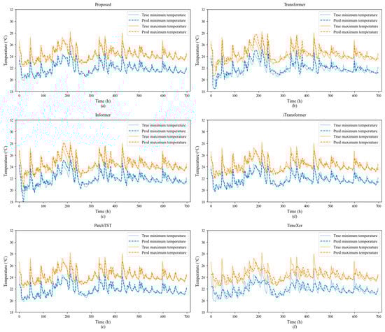
Figure 4.
Illustrative comparison of prediction results for each model regarding Dataset 1. In the figure, the solid blue line represents the ground truth of minimum temperature, the dashed blue line represents the predicted minimum temperature, the solid yellow line represents the ground truth of maximum temperature, and the dashed yellow line represents the predicted maximum temperature. Each subplot corresponds to the prediction results of a different model: (a) the proposed method, (b) Transformer, (c) Informer, (d) iTransformer, (e) PatchTST, and (f) TimeXer.
As can be seen from Figure 4, for 1-step-ahead prediction, the proposed method demonstrates excellent tracking between predicted and actual values. During minor data fluctuations, the predicted and actual values align closely, and the method responds quite sensitively to local data variations. However, at higher peak values, the proposed method tends to underestimate these peaks; nevertheless, these errors remain around approximately 2 °C, which is within an acceptable range.
The Transformer model performed poorly in predicting minor fluctuations and was sluggish in responding to minor local changes. It exhibited significant prediction bias around the 0th to 20th sampling points and near the 170th to 220th sampling points. The Informer model also showed notable prediction bias around the 5th to 20th sampling points and near the 170th to 210th sampling points, which may be indicative of the poorer results obtained by the Transformer and Informer models shown in Table 2. The iTransformer model also exhibited sensitivity to local changes, but it underestimated many minor peaks. PatchTST also demonstrated sensitivity to local data variations, a characteristic closely related to its excellent ability to extract local temporal features. However, its underestimation of some peaks is more pronounced than that of the proposed method. Although TimeXer can capture local data fluctuations reasonably well, its overall estimations of numerical values at each sampling point are generally poor.
To provide a more comprehensive evaluation of each model’s prediction performance for the upcoming 24 h of data, we present, using Dataset 1 as an example, box plots of the prediction errors for each model at every time step within the prediction window. Detailed information is shown in Figure 5. To ensure the clarity and conciseness of the subplots, outliers are not displayed in the figure.

Figure 5.
Box plots of prediction errors for each model with respect to Dataset 1 at each prediction time step. In each row, the left plot shows the box plot of prediction errors for the minimum temperature, and the right plot shows the box plot of prediction errors for the maximum temperature. The short red line segments within the plots indicate the median prediction error. (a,b) the proposed method; (c,d) Transformer; (e,f) Informer; (g,h) iTransformer; (i,j) PatchTST; and (k,l) TimeXer.
According to Figure 5, the median prediction error of the proposed method is close to zero across all time steps, indicating that the model exhibits low systematic bias in temperature prediction. As the prediction horizon increases, the interquartile range (IQR) and the length of the whiskers gradually increase, stabilizing after the fifth time step. The error distribution remains relatively stable and compact. The whisker tips are situated around ±2 °C, which is within an acceptable range.
The median prediction error of the Transformer model is slightly above zero at almost all time steps, indicating a systematic overestimation in its predictions; this overestimation appears more pronounced in the prediction of the maximum temperature. The IQR and whisker length also gradually increase with the prediction step, and the error dispersion for the Transformer model is slightly greater than that for the proposed method. The Informer model’s errors are relatively compact before the sixth prediction step; however, its predictions exhibit systematic overestimation. The median prediction error of the iTransformer model consistently stays near zero, indicating it has minimal systematic prediction bias. However, the compactness of its errors at later time steps is slightly inferior to that of the proposed method. The median prediction error of the PatchTST model is also relatively close to zero, exhibiting low systematic prediction bias, while the compactness of its errors at later time steps is inferior to that of the proposed method. The median prediction error of the TimeXer model remains near zero; however, the dispersion of its errors at earlier time steps is noticeably higher than that of other models. This aligns with the prediction performance depicted in Figure 4. Overall, the magnitude of its errors is slightly higher than that of the other models.
Furthermore, the optimal results reported for the aforementioned comparative models in the 24-step prediction experiments were achieved after experimenting with various truncated look-back windows. In practical application scenarios where future label data is unavailable, the process of obtaining different results from multiple predictions could inherently introduce interference for decision-makers, making it difficult for them to determine which result is the most reliable. In contrast, the method proposed in this paper only requires accepting the long look-back window directly, and it can automatically extract its multi-scale periodic features and local temporal characteristics, thereby minimizing such interference for decision-makers.
In summary, it can be asserted that the method proposed in this paper not only demonstrates commendable accuracy and prediction stability in the comparative experiments but is also more suitable for providing a reliable basis for decision-making in practical scenarios.
4.4. Comparative Experiments for Other Prediction Horizons
To evaluate the performance of the proposed model under different prediction horizon scenarios, we conducted comparative experiments for 48 h and 72 h predictions. Similar to the classic 24 h prediction, for each comparative model, in addition to evaluating performance using a look-back window of 24 × 7 sampling points, we also conducted experiments by truncating data from the end of this window to construct new, shorter look-back windows. For the 48 h prediction experiments, the final test results for the two datasets are presented in Table 4 and Table 5, respectively. Similarly, for the 72 h prediction experiments, the results for the two datasets are shown in Table 6 and Table 7, respectively. All metrics in these tables are also reported as the means ± standard deviations over five runs.
Table 4.
Comparative results for 48 h prediction with respect to Dataset 1.
Table 5.
Comparative results for 48 h prediction using Dataset 2.
Table 6.
Comparative results for 72 h prediction with respect to Dataset 1.
Table 7.
Comparative results for 72 h prediction with respect to Dataset 2.
According to Table 4 and Table 5, the proposed model continued to achieve the best test results, and its stability also remained high. As with the classic 24 h prediction, iTransformer and PatchTST still yielded good test results, and their overall performances were comparable. The stability of the Transformer and Informer models was also relatively poor. TimeXer, on the other hand, yielded moderate performance overall.
In Table 2, Table 3, Table 4 and Table 5, it can be observed that as the prediction horizon increased, the prediction performance of all the models declined, which aligns with the general pattern in time series forecasting. When the prediction time was extended from 24 h to 48 h, for Dataset 1, the average MSE, MAE, and RMSE values of the proposed model degraded by 14.56%, 8.12%, and 7.03%, respectively. The three average metrics for iTransformer at its best performance degraded by 22.63%, 12.04%, and 10.74%, respectively, and those for PatchTST at its best performance degraded by 20.87%, 12.21%, and 9.94%, respectively. For Dataset 2, the average MSE, MAE, and RMSE values of the proposed model degraded by 28.34%, 15.64%, and 13.29%, respectively. The three average metrics for iTransformer at its best performance degraded by 33.79%, 17.07%, and 15.67%, respectively, while those for PatchTST at its best performance degraded by 33.69%, 18.55%, and 15.62%, respectively.
According to Table 6 and Table 7, the proposed model continued to achieve the best average evaluation metrics, and its stability also remained at a high level. After the prediction horizon was extended from 24 h to 72 h, for Dataset 1, the average MSE, MAE, and RMSE values of the proposed model degraded by 25.29%, 14.19%, and 11.93%, respectively. The three average metrics for iTransformer at its best performance degraded by 39.83%, 22.59%, and 18.25%, respectively, while those for PatchTST at its best performance degraded by 33.38%, 18.35%, and 15.49%, respectively. For Dataset 2, the average MSE, MAE, and RMSE values of the proposed model degraded by 43.31%, 23.50%, and 19.71%, respectively. The three average metrics for iTransformer at its best performance degraded by 53.35%, 25.88%, and 23.83%, respectively, while those for PatchTST at its best performance degraded by 50.98%, 26.95%, and 22.88%, respectively.
Based on the metrics, iTransformer and PatchTST were consistently strong competitors with respect to the model proposed in this paper. However, iTransformer primarily focuses on the overall characteristics of the time series and the correlations between monitored variables, whereas PatchTST places greater emphasis on local variations within the time series. The model proposed in this paper can concurrently address inter-variable correlations, the multi-scale periodic characteristics of time series, and local variations within time series. Consequently, the model described herein consistently achieved the best results in terms of evaluation metrics. Furthermore, the aforementioned figures regarding the degree of model degradation also indicate that when the prediction horizon lengthens, the performance decay exhibited by the algorithm proposed in this paper is significantly less than that of iTransformer and PatchTST. This further demonstrates the superiority of the model described in this paper in handling prediction tasks of varying lengths.
4.5. Ablation Study
To further demonstrate the positive contribution of each module to the prediction task, ablation studies were conducted in this paper. It is noteworthy that, similar to the comparative experiments section, each model in the ablation study was also run 5 times with different random seeds. Furthermore, when experimenting without the CNN Block, new look-back windows were constructed by truncating data from the end of the original look-back window. It is also important to note that during the ablation study of the KAN module, an MLP was used to replace the original single-layer KAN model. Table 8 and Table 9 list the average statistical metrics and prediction deviations obtained from the ablation studies conducted on Dataset 1 and Dataset 2, respectively.
Table 8.
Ablation results regarding Dataset 1.
Table 9.
Ablation results for Dataset 2.
The results presented in Table 8 and Table 9 indicate that each module of the proposed method is crucial. When an MLP was used instead of the KAN model in the final layer, the average values of the MSE, MAE, and RMSE all showed degradation, and a noticeable degradation in stability was also observed in the classic 24 h prediction. This suggests that the KAN model successfully parsed future information embedded in the complex, multi-dimensional encoded representations from the preceding stages. Upon removing patch embedding, the average values of all the evaluation metrics exhibited greater degradation. Simultaneously, except for the 48 h prediction on Dataset 2, removing patch embedding led to a significant decrease in model stability in all cases. This indicates that local temporal variations embedded within different segments of the long look-back window constitute critical information for the BESS temperature prediction process. Finally, after removing the CNN block, regardless of how the look-back window was truncated, the average values of the evaluation metrics showed a decline. This demonstrates that the multi-scale periodic features embedded in the long look-back window, as well as the correlation information between various monitoring variables, are also critical for the BESS temperature prediction process.
5. Conclusions and Prospects
5.1. Conclusions
In this paper, we propose a BESS temperature prediction method based on the CNN–Patch–Transformer model. In this method, a CNN block is used to extract multi-scale periodic features from historical data and capture the multi-scale correlations among various monitored variables. Patch embedding, combined with an attention module, is employed to extract local variation features from the temporal data. The KAN model is then utilized to map the acquired multi-dimensional information, thereby achieving joint prediction of the maximum and minimum temperatures of a BESS.
In the experimental phase, we conducted a comparative analysis against Transformer, Informer, iTransformer, PatchTST, and TimeXer models. The experimental results demonstrate that the proposed method can automatically extract key information that is conducive to prediction from long historical look-back windows. In comparative experiments conducted across different prediction horizons, the values obtained for the statistical metrics MSE, MAE, and RMSE consistently exhibited the best evaluation performance. The results of ablation studies also validated the positive contribution of each component in the proposed method. The findings from various experiments also indicate that for temperature prediction in practical BESS scenarios, the multi-scale periodic features of time series data, local variation characteristics, and the correlations among monitored variables are all crucial factors for ensuring prediction accuracy.
5.2. Prospects
Due to the datasets employed in this study not directly providing detailed BESS charge/discharge state labels, an analysis based on operational modes was not undertaken at this stage. Furthermore, as the datasets span a period of one year, an error analysis based on seasonal patterns was also omitted to mitigate the risk of drawing potentially biased conclusions from imbalanced data across seasons. Consequently, an important direction for future research will be the collection or annotation of datasets that include explicit seasonal information and detailed BESS operating conditions. This will enable a meticulous quantitative evaluation of the proposed model’s performance under diverse conditions, and such fine-grained analysis will be invaluable for developing more robust models tailored to complex, real-world operating scenarios and further enhancing their practical utility.
Given the availability of relevant data, the findings of this research are based on residential BESS datasets. However, the constituent components of the proposed model are designed to capture fundamental characteristics within time series data, and these characteristics are also likely present in monitoring data from industrial and utility-scale BESSs, although their specific manifestations in terms of magnitude and parameters may vary. Consequently, the core architecture of the proposed model possesses inherent potential for generalizability and scalability. Future work will be dedicated to retraining and fine-tuning the model using data from systems of specific scales to extend its applicability to a wider range of BESS application scenarios.
Another significant avenue for future research will involve the practical deployment of this model. While the current work has established its predictive superiority, the computational burden and inference latency in real-time BESS applications remain to be thoroughly evaluated. The complexity introduced by the CNN block, transformer encoder, and KAN layer suggests that direct implementation in resource-constrained embedded BESS controllers could be challenging without optimization. Therefore, future investigations will explore techniques such as model pruning, quantization, and knowledge distillation to create more lightweight and efficient versions of the model and deploy and optimize these versions on representative embedded hardware platforms commonly used in BESSs. Furthermore, in practical scenarios, leveraging predicted temperature to guide the establishment of effective thermal management strategies, charge/discharge management policies, and early fault diagnosis will be crucial for enabling this model to meet real-world application demands. This will represent a key step in transforming this research into a practical tool for BESS thermal management.
Author Contributions
Conceptualization, Y.L. and K.Q.; methodology, Y.L. and K.Q.; software, Y.L.; validation, K.Q., Q.S., and Q.M.; formal analysis, Q.S. and Q.M.; investigation, X.W.; resources, Y.L. and K.Q.; data curation, X.W. and Z.W.; writing—original draft preparation, Y.L.; writing—review and editing, X.W. and Z.W.; visualization, Z.W.; supervision, K.Q.; project administration, K.Q.; funding acquisition, K.Q. All authors have read and agreed to the published version of the manuscript.
Funding
This work is supported by Science and Technology Project Funding of State Grid Jiangsu Electric Power Co., Ltd. (J2024015).
Data Availability Statement
The data presented in this study are available on request from the corresponding author. The data are not publicly available due to privacy concerns.
Conflicts of Interest
Authors Yafei Li, Kejun Qian, Qiuying Shen and Qianli Ma were employed by the State Grid Suzhou Power Supply Company. The remaining authors declare that the research was conducted in the absence of any commercial or financial relationships that could be construed as a potential conflict of interest. The authors declare that this study received funding from State Grid Jiangsu Electric Power Co., Ltd. The funder was not involved in the study design, collection, analysis, interpretation of data, the writing of this article or the decision to submit it for publication.
Abbreviations
The following abbreviations are used in this manuscript:
| BESS | Battery Energy Storage System |
| SOH | State of Health |
| BMS | Battery Management System |
| BP-NN | Backpropagation Neural Network |
| RBF-NN | Radial Basis Function Neural Network |
| Elman-NN | Elman Neural Network |
| EGA | Elitist Genetic Algorithm |
| BiLSTM | Bidirectional Long Short-Term Memory |
| LightGBM | Light Gradient Boosting Machine |
| CNN | Convolutional Neural Network |
| AM | Attention Mechanism |
| RUL | Remaining Useful Life |
| EMD | Empirical Mode Decomposition |
| IMF | Intrinsic Mode Function |
| EV | Electric Vehicle |
| SS-ANN | Spiral Self-Attention Neural Network |
| SAM | Self-Attention Mechanism |
| GRU | Gated Recurrent Unit |
| KAN | Kolmogorov–Arnold Network |
| MSE | Mean Squared Error |
| FFN | Feed-Forward Network |
| MLP | Multilayer Perceptron |
| SOC | State of Charge |
| LFP | Lithium Iron Phosphate |
| LOF | Local Outlier Factor |
| MAE | Mean Absolute Error |
| RMSE | Root Mean Square Error |
| PatchTST | Patch Time Series Transformer |
| TimeXer | Time Series Transformer with Exogenous Variables |
| TSLib | Time Series Library |
| IQR | Interquartile Range |
References
- Gao, Y.; Xing, F.; Kang, L.; Zhang, M.; Qin, C. Ultra-Short-Term Wind Power Prediction Based on the ZS-DT-PatchTST Combined Model. Energies 2024, 17, 4332. [Google Scholar] [CrossRef]
- Bracale, A.; De Falco, P.; Noia, L.P.D.; Rizzo, R. Probabilistic State of Health and Remaining Useful Life Prediction for Li-Ion Batteries. IEEE Trans. Ind. Appl. 2023, 59, 578–590. [Google Scholar] [CrossRef]
- Wang, S.; Zhao, L.; Su, X.; Ma, P. Prognostics of Lithium-Ion Batteries Based on Battery Performance Analysis and Flexible Support Vector Regression. Energies 2014, 7, 6492–6508. [Google Scholar] [CrossRef]
- Wang, Y.; Xiong, C.; Wang, Y.; Xu, P.; Ju, C.; Shi, J.; Yang, G.; Chu, J. Temperature State Prediction for Lithium-Ion Batteries Based on Improved Physics Informed Neural Networks. J. Energy Storage 2023, 73, 108863. [Google Scholar] [CrossRef]
- Chu, F.; Shan, C.; Guo, L. Temporal Attention Mechanism Based Indirect Battery Capacity Prediction Combined with Health Feature Extraction. Electronics 2023, 12, 4951. [Google Scholar] [CrossRef]
- Chen, J.; Zhao, Y.; Wang, M.; Yang, K.; Ge, Y.; Wang, K.; Lin, H.; Pan, P.; Hu, H.; He, Z.; et al. Multi-Timescale Reward-Based DRL Energy Management for Regenerative Braking Energy Storage System. IEEE Trans. Transp. Electrif. 2025, 11, 7488–7500. [Google Scholar] [CrossRef]
- Ying, Y.; Tian, Z.; Wu, M.; Liu, Q.; Tricoli, P. A Real-Time Energy Management Strategy of Flexible Smart Traction Power Supply System Based on Deep Q-Learning. IEEE Trans. Intell. Transp. Syst. 2024, 25, 8938–8948. [Google Scholar] [CrossRef]
- Zhang, H.; Fotouhi, A.; Auger, D.J.; Lowe, M. Battery Temperature Prediction Using an Adaptive Neuro-Fuzzy Inference System. Batteries 2024, 10, 85. [Google Scholar] [CrossRef]
- Fan, X.; Zhang, W.; Qi, H.; Zhou, X. Accurate Battery Temperature Prediction Using Self-Training Neural Networks within Embedded System. Energy 2024, 313, 134031. [Google Scholar] [CrossRef]
- Zhang, W.; Wan, W.; Wu, W.; Zhang, Z.; Qi, X. Internal Temperature Prediction Model of the Cylindrical Lithium-Ion Battery under Different Cooling Modes. Appl. Therm. Eng. 2022, 212, 118562. [Google Scholar] [CrossRef]
- Krewer, U.; Röder, F.; Harinath, E.; Braatz, R.D.; Bedürftig, B.; Findeisen, R. Review—Dynamic Models of Li-Ion Batteries for Diagnosis and Operation: A Review and Perspective. J. Electrochem. Soc. 2018, 165, A3656. [Google Scholar] [CrossRef]
- Wang, Y.; Chen, X.; Li, C.; Yu, Y.; Zhou, G.; Wang, C.; Zhao, W. Temperature Prediction of Lithium-Ion Battery Based on Artificial Neural Network Model. Appl. Therm. Eng. 2023, 228, 120482. [Google Scholar] [CrossRef]
- Jiang, L.; Yan, C.; Zhang, X.; Zhou, B.; Cheng, T.; Zhao, J.; Gu, J. Temperature Prediction of Battery Energy Storage Plant Based on EGA-BiLSTM. Energy Rep. 2022, 8, 1009–1018. [Google Scholar] [CrossRef]
- Zhao, H.; Chen, Z.; Shu, X.; Xiao, R.; Shen, J.; Liu, Y.; Liu, Y. Online Surface Temperature Prediction and Abnormal Diagnosis of Lithium-Ion Batteries Based on Hybrid Neural Network and Fault Threshold Optimization. Reliab. Eng. Syst. Saf. 2024, 243, 109798. [Google Scholar] [CrossRef]
- Zhao, H.; Xu, P.; Gao, T.; Zhang, J.J.; Xu, J.; Gao, D.W. CPTCFS: CausalPatchTST Incorporated Causal Feature Selection Model for Short-Term Wind Power Forecasting of Newly Built Wind Farms. Int. J. Electr. Power Energy Syst. 2024, 160, 110059. [Google Scholar] [CrossRef]
- Li, L.; Li, Y.; Mao, R.; Li, L.; Hua, W.; Zhang, J. Remaining Useful Life Prediction for Lithium-Ion Batteries With a Hybrid Model Based on TCN-GRU-DNN and Dual Attention Mechanism. IEEE Trans. Transp. Electrif. 2023, 9, 4726–4740. [Google Scholar] [CrossRef]
- Wang, Y.; Jiang, B. Attention Mechanism-Based Neural Network for Prediction of Battery Cycle Life in the Presence of Missing Data. Batteries 2024, 10, 229. [Google Scholar] [CrossRef]
- Sun, S.; Sun, J.; Wang, Z.; Zhou, Z.; Cai, W. Prediction of Battery SOH by CNN-BiLSTM Network Fused with Attention Mechanism. Energies 2022, 15, 4428. [Google Scholar] [CrossRef]
- Lin, M.; Wu, J.; Meng, J.; Wang, W.; Wu, J. State of Health Estimation with Attentional Long Short-Term Memory Network for Lithium-Ion Batteries. Energy 2023, 268, 126706. [Google Scholar] [CrossRef]
- Li, C.; Kong, Y.; Wang, C.; Wang, X.; Wang, M.; Wang, Y. Relevance-Based Reconstruction Using an Empirical Mode Decomposition Informer for Lithium-Ion Battery Surface-Temperature Prediction. Energies 2024, 17, 5001. [Google Scholar] [CrossRef]
- Qi, X.; Hong, C.; Ye, T.; Gu, L.; Wu, W. Frequency Reconstruction Oriented EMD-LSTM-AM Based Surface Temperature Prediction for Lithium-Ion Battery. J. Energy Storage 2024, 84, 111001. [Google Scholar] [CrossRef]
- Hong, J.; Zhang, H.; Xu, X. Thermal Fault Prognosis of Lithium-Ion Batteries in Real-World Electric Vehicles Using Self-Attention Mechanism Networks. Appl. Therm. Eng. 2023, 226, 120304. [Google Scholar] [CrossRef]
- Nie, Y.; Nguyen, N.H.; Sinthong, P.; Kalagnanam, J. A Time Series Is Worth 64 Words: Long-Term Forecasting with Transformers. arXiv 2023, arXiv:2211.14730. [Google Scholar] [CrossRef]
- Wang, Y.; Wu, H.; Dong, J.; Liu, Y.; Long, M.; Wang, J. Deep Time Series Models: A Comprehensive Survey and Benchmark. arXiv 2024, arXiv:2407.13278. [Google Scholar] [CrossRef]
- Vaswani, A.; Shazeer, N.; Parmar, N.; Uszkoreit, J.; Jones, L.; Gomez, A.N.; Kaiser, L.; Polosukhin, I. Attention Is All You Need. arXiv 2023, arXiv:1706.03762. [Google Scholar] [CrossRef]
- Han, X.; Zhang, X.; Wu, Y.; Zhang, Z.; Wu, Z. Are KANs Effective for Multivariate Time Series Forecasting? arXiv 2025, arXiv:2408.11306. [Google Scholar] [CrossRef]
- Liu, Z.; Wang, Y.; Vaidya, S.; Ruehle, F.; Halverson, J.; Soljačić, M.; Hou, T.Y.; Tegmark, M. KAN: Kolmogorov-Arnold Networks. arXiv 2025, arXiv:2404.19756. [Google Scholar] [CrossRef]
- Yu, R.; Yu, W.; Wang, X. KAN or MLP: A Fairer Comparison. arXiv 2024, arXiv:2407.16674. [Google Scholar] [CrossRef]
- Breunig, M.M.; Kriegel, H.-P.; Ng, R.T.; Sander, J. LOF: Identifying Density-Based Local Outliers. In Proceedings of the 2000 ACM SIGMOD International Conference on Management of Data; Association for Computing Machinery: New York, NY, USA, 2000; pp. 93–104. [Google Scholar]
- Zhou, H.; Zhang, S.; Peng, J.; Zhang, S.; Li, J.; Xiong, H.; Zhang, W. Informer: Beyond Efficient Transformer for Long Sequence Time-Series Forecasting. Proc. AAAI Conf. Artif. Intell. 2021, 35, 11106–11115. [Google Scholar] [CrossRef]
- Liu, Y.; Hu, T.; Zhang, H.; Wu, H.; Wang, S.; Ma, L.; Long, M. iTransformer: Inverted Transformers Are Effective for Time Series Forecasting. arXiv 2024, arXiv:2310.06625. [Google Scholar] [CrossRef]
- Wang, Y.; Wu, H.; Dong, J.; Qin, G.; Zhang, H.; Liu, Y.; Qiu, Y.; Wang, J.; Long, M. TimeXer: Empowering Transformers for Time Series Forecasting with Exogenous Variables. arXiv 2024, arXiv:2402.19072. [Google Scholar] [CrossRef]
- Liu, Y.; Wu, H.; Wang, J.; Long, M. Non-Stationary Transformers: Exploring the Stationarity in Time Series Forecasting. arXiv 2023, arXiv:2205.14415. [Google Scholar] [CrossRef]
Disclaimer/Publisher’s Note: The statements, opinions and data contained in all publications are solely those of the individual author(s) and contributor(s) and not of MDPI and/or the editor(s). MDPI and/or the editor(s) disclaim responsibility for any injury to people or property resulting from any ideas, methods, instructions or products referred to in the content. |
© 2025 by the authors. Licensee MDPI, Basel, Switzerland. This article is an open access article distributed under the terms and conditions of the Creative Commons Attribution (CC BY) license (https://creativecommons.org/licenses/by/4.0/).