1. Introduction
Energy underpins national development, and its secure and stable supply is essential for economic growth and social stability. In recent decades, wind energy as a typical form of clean power has seen rapid adoption and has contributed significantly to carbon emissions reduction and sustainable development. Nevertheless, the inherent intermittency and variability of wind energy introduce notable challenges to the stable operation of modern power systems [
1,
2,
3,
4]. Therefore, enhancing the ability to predict wind energy output accurately is of great importance for strengthening grid stability, improving energy system efficiency, and supporting long-term sustainability goals [
5,
6,
7,
8]. Current research focuses on improving the accuracy and reliability of wind power prediction to provide strong support for the stable development of the energy industry.
Wind power prediction methods mainly include physical, statistical, and artificial intelligence-based approaches. Physics-based approaches were the earliest techniques used for wind power prediction, relying on numerical weather prediction (NWP) models and physical data [
9]. Reference [
10] proposed a method integrating overlapping historical NWP datasets to improve intraday wind power prediction accuracy. By incorporating historical NWP data and employing an innovative representation learning pretraining strategy, this model effectively captured spatiotemporal correlations and enhanced prediction accuracy. However, physics-based models struggle with extreme weather adaptability, suffer from high computational complexity, and heavily depend on high-quality meteorological data, limiting their applicability in highly dynamic environments.
Statistical approaches primarily rely on historical data and the statistical relationships between meteorological factors and wind power generation. Common techniques include time series analysis, regression analysis, and Bayesian inference. By modeling wind speed, wind direction, temperature, and other meteorological factors, statistical models can capture the variation patterns of wind power. Reference [
11] optimized the autoregressive integrated moving average (ARIMA) model with an enhancement scheme for short-term load prediction, while Reference [
12] improved the ARIMA model using repeated wavelet transform, enhancing wind speed prediction accuracy. Although statistical methods offer good interpretability, their prediction accuracy declines significantly in extreme weather conditions, large-scale meteorological fluctuations, or missing data scenarios. Additionally, they heavily depend on data quality and struggle to capture the complex nonlinear variations in wind power, necessitating integration with other models to enhance robustness.
With advancements in artificial intelligence, machine learning techniques have been widely applied in wind power prediction. Reference [
13] proposed a model based on random forest regression (RFR) to enhance nonlinear feature representation. Reference [
14] employed support vector machines (SVMs) with wavelet transform for noise reduction and cuckoo search for parameter optimization, improving prediction accuracy. Reference [
15] integrated the light gradient boosting machine (LightGBM) with the mutual information coefficient (MIC) for key meteorological feature selection, enhancing nonlinear fitting capability. However, traditional machine learning models struggle with long-term dependency modeling and temporal feature extraction. Additionally, their performance heavily relies on manual feature selection and hyperparameter tuning, which limits model generalization.
Deep learning models automatically extract complex nonlinear relationships from data, exhibiting strong adaptability. Reference [
16] employed an long short-term memory (LSTM)-based model combined with MIC and multitask learning (MTL) to enhance the relationship modeling between wind speed and wind power. Reference [
17] introduced a temporal convolutional network (TCN)-based model that utilized dilated causal convolutions and residual connections to improve long-term dependency modeling. Reference [
18] introduced a gated recurrent unit (GRU)-based model for building a smart wind power prediction system, emphasizing its effectiveness in modeling time series features and adaptability to low-resource environments. Reference [
19] proposed a Transformer-based wind power prediction model that utilized self-attention mechanisms to capture long-range dependencies and enhance sequence modeling capabilities. Reference [
20] applied a multilayer perceptron (MLP) model with NWP and supervisory control and data acquisition (SCADA) inputs for wind power prediction, supporting market scheduling decisions. Although deep learning models have advanced significantly, they still face key limitations in practical use. Their reliance on large labeled datasets, high computational costs, and lack of interpretability hinder their application in real-time and transparent wind power prediction. Thus, there is a clear need for models that balance accuracy, efficiency, and interpretability.
To overcome the limitations of single models in wind power prediction, recent research has not only focused on improving model structures but also increasingly emphasized the importance of effective feature processing. High-quality input features are crucial for enhancing models’ ability to learn complex temporal patterns and improve prediction accuracy. As a result, various advanced feature engineering techniques have been introduced [
21,
22]. For example, Reference [
23] incorporated chaotic disturbance noise to enrich the distribution of power features, while ref. [
24] applied complete ensemble empirical mode decomposition with adaptive noise (CEEMDAN) to decompose wind signals into trend and periodic components. Reference [
25] used variational mode decomposition (VMD) to extract stationary sub-series, and ref. [
26] employed fast Fourier transform (FFT) to uncover hidden periodic structures in the frequency domain. However, these methods still face challenges such as poor adaptability to non-stationary signals, high computational complexity, sensitivity to parameter settings, and difficulty capturing short-term volatility in small datasets—leading to potential overfitting and reduced prediction performance.
Wind power prediction models are highly sensitive to hyperparameter configurations, and traditional tuning methods often suffer from inefficiency and local optima issues. To improve optimization efficiency, bioinspired optimization algorithms have been introduced. Reference [
27] employed the whale optimization algorithm (WOA) to optimize kernel extreme learning machine (KELM) parameters, enhancing prediction accuracy. Reference [
28] utilized an improved dung beetle optimization (IDBO) algorithm to optimize VMD parameters, improving data decomposition stability. Reference [
29] introduced an improved reptile search algorithm (IRSA) to optimize bidirectional long short-term memory (BiLSTM) and extreme learning machine (ELM) hyperparameters, improving global optimization and model accuracy. However, bioinspired optimization algorithms generally entail high computational costs and limited generalization across different datasets, requiring further enhancements to improve their stability and adaptability.
To improve the generalization and interpretability of wind power prediction models under complex conditions, this study proposes a lightweight modeling approach integrating multi-source features. Drawing inspiration from financial time series analysis [
30], the model incorporates candlestick (K-line) structures and three classical indicators—moving average convergence divergence (MACD), Bollinger bands (BOLL), and average true range (ATR)—to characterize trend, volatility, and short-term dynamics. It also introduces power fluctuation features based on current, lagged, and differential power values to enhance responsiveness to abrupt changes. The extreme gradient boosting (XGBoost) algorithm is employed for prediction, offering a favorable balance of accuracy, computational efficiency, and model transparency. Its tree-based structure enables the effective interpretation of feature contributions, supporting practical deployment in volatile prediction scenarios. Compared with most deep learning models, the proposed method achieves comparable predictive performance while significantly reducing model complexity and improving interpretability and deployment flexibility.
To evaluate the effectiveness and generalization capability of the proposed method, initial experiments were conducted using real-world data from a wind farm in Inner Mongolia, a region characterized by abundant wind resources and complex meteorological conditions. This area is one of the most representative regions for wind power prediction research in China. Wang et al. [
31] also conducted a study based on data from this region, proposing a hybrid prediction model that integrates improved entropy weighting, selective ensemble complete empirical mode decomposition (SECEEMD) decomposition, and deep learning. Compared with their approach, the method proposed in this study achieves comparable prediction accuracy while significantly reducing model complexity, improving modeling efficiency, and enhancing interpretability. Furthermore, to assess cross-regional generalization, the model was also tested on wind power data from the European network of transmission system operators for electricity (ENTSO-E) dataset in Germany. The results similarly demonstrated strong predictive performance, confirming the robustness and transferability of the proposed method. Overall, this study presents a practical, lightweight, and interpretable framework for wind power prediction, demonstrating a promising application of financial analysis techniques in the energy domain.
2. Model Framework and Key Algorithms
2.1. Model Framework
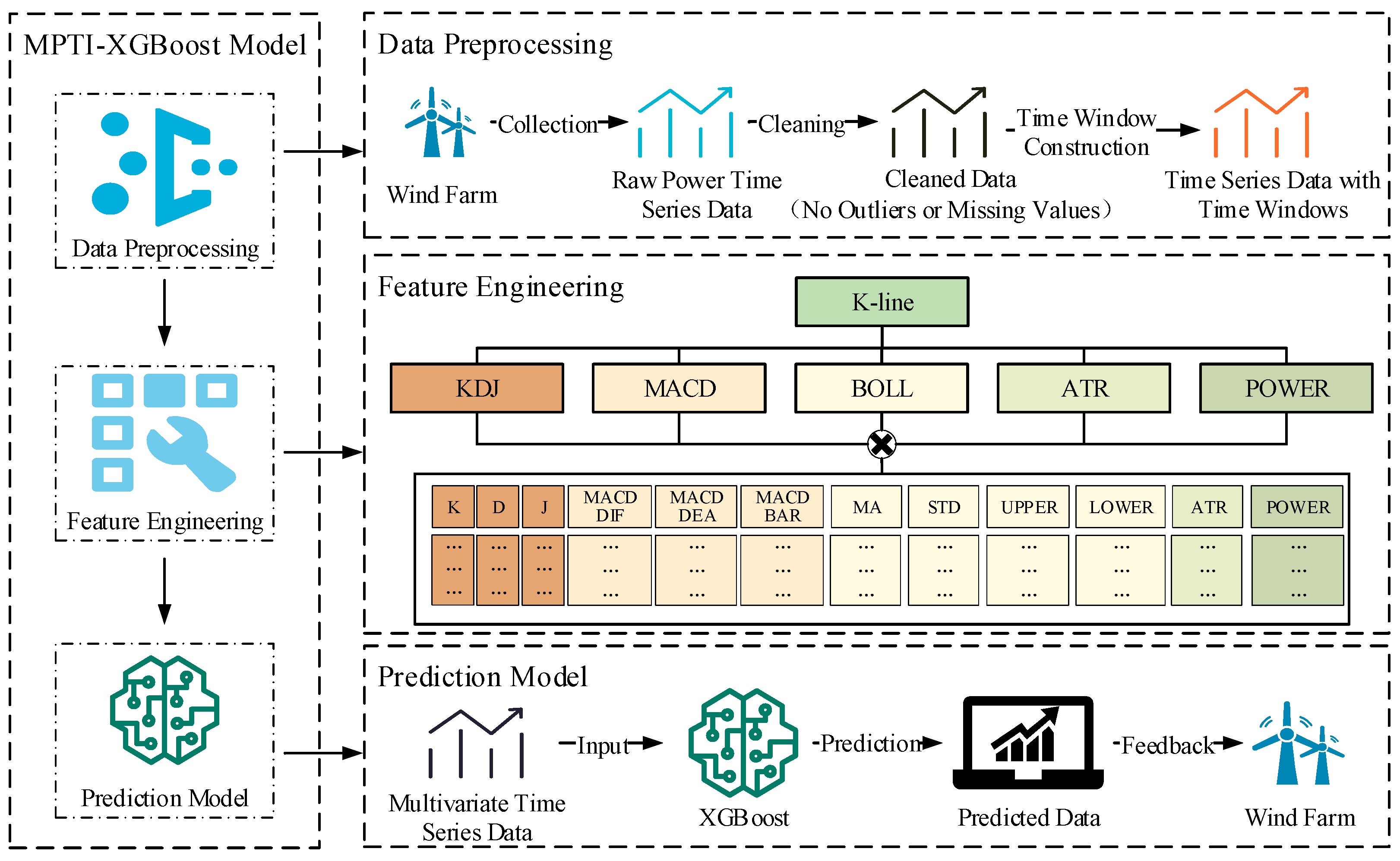
To improve the accuracy and reliability of wind power prediction, this study proposes a wind power prediction method that integrates multiple technical indicators and the XGBoost algorithm, named multiple technical indicators and XGBoost (MTI-XGBoost). As shown in
Figure 1, the prediction process of the MTI-XGBoost model is primarily divided into three modules: data preprocessing, feature engineering, and the prediction model.
First, during the preprocessing phase, the power data from the wind farm is carefully processed to improve data reliability by eliminating anomalies, thereby minimizing their impact on model learning. Meanwhile, a sliding window approach is employed to capture the initial, maximum, minimum, and final power values within each time interval, providing the basis for later-stage feature construction and analysis.
Next, in the feature engineering module, multiple technical indicators and power fluctuation features are extracted based on the preprocessed time window power data. First, a power candlestick chart is drawn, similar to the candlestick charts in financial markets, to visually present power fluctuations. Then, three technical indicators are calculated—MACD, BOLL, and ATR—which are used to analyze trend reversals, fluctuation ranges, and fluctuation amplitudes, respectively. Additionally, power fluctuation features are introduced by recording the current power value, the previous power value, and their difference to capture short-term power changes. The combination of these features and technical indicators significantly improves the model’s sensitivity to power fluctuations and prediction accuracy.
In the prediction model module, the processed multi-feature data is divided into training and testing sets and input into the XGBoost model for training. Finally, the prediction results are fed back into the wind farm management system, providing reliable power predictions to support operational scheduling and optimization decisions.
2.2. Construction of Sliding Time Window
To further explore the features of wind power time series data, this study adopts the time window method to expand the dimensionality of the input data. First, analyzing the periodic characteristics of wind power, the sampling interval is set to 15 min, and five consecutive sampling points are combined into a single data unit. Next, a sliding time window is used to sequentially construct time series samples: the first to fifth sampling points form the first sample, the second to sixth sampling points form the second sample, and so on. This method transforms the original data into a periodic time series dataset. Finally, power features, including the starting value, highest value, lowest value, and ending value, are extracted from each time window, providing foundational data for subsequent analysis and model construction.
2.3. Power Fluctuation Features
To capture deeper characteristics of wind power time series, this paper applies a sliding window approach to increase the feature space of the input. These features record the current power value, the previous power value, and their difference, thereby revealing the short-term change trends in wind power and providing key dynamic information for the model. Specifically, power fluctuation characteristics are calculated using the following equation:
In the formula, represents the wind power value at the current time, represents the power value at the previous time, and is the power fluctuation, which is the difference in power between the two time points.
By recording the power value and its fluctuation at each moment, the model can identify the trends of power increase, decrease, or stability. Due to the high volatility and uncertainty of wind power over short periods, these fluctuation features, when used as inputs to the model and combined with other technical indicators and time series data, help to significantly improve the prediction accuracy of the model.
2.4. Candlestick Chart Based on Power Time Series Data
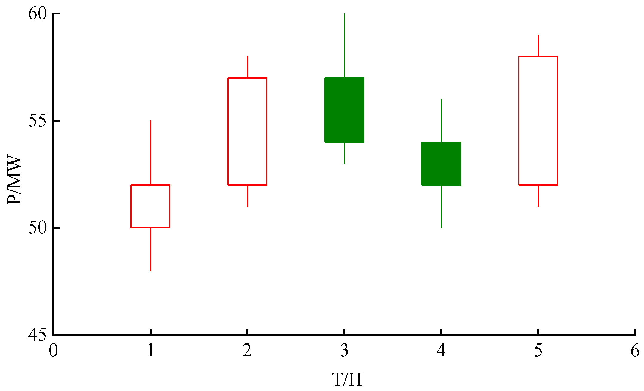
In financial markets, candlestick charts are drawn using the opening price, highest price, lowest price, and closing price. If the opening price is higher than the closing price, the candlestick is represented by a filled body; if the opening price is lower than the closing price, the candlestick is represented by an empty body. A candlestick chart based on wind power data is shown in
Figure 2 (where P represents power in MW and T represents the collection time in hours). In this figure, red hollow candlesticks indicate periods of increasing wind power, while green solid candlesticks indicate periods of decreasing wind power.
In this study, a candlestick chart approach is introduced for modeling wind power time series. Referring to the sliding window framework outlined in
Section 2.2, the power reading at the beginning of each window is regarded as the “opening” value, while the maximum and minimum readings represent the “high” and “low” values, respectively, and the final point in the window corresponds to the “closing” value. This graphical structure captures fluctuations in wind power by visualizing opening, high, low, and closing values over time intervals, and serves as the foundation for calculating subsequent technical indicators.
2.5. Moving Average Convergence Divergence Based on Power Time Series Data
The Moving Average Convergence Divergence indicator, also known as MACD, was developed by Gerald Appel and is a classical trend-following technique originally used in financial time series analysis [
32]. This study introduces the MACD indicator into wind power prediction to capture trend variations in power data by combining the principles of oscillators with a new crossover method involving the exponential moving average (EMA). The method consists of the Fast Line difference (DIF), Slow Line differential exponential average (DEA), and the Red–Green Histogram buyer acceptance range (BAR). The key to this method lies in the relationship between the short-term and long-term exponential moving averages. In this study, the short-term and long-term EMAs use 3- and 5-period time windows, respectively, to better capture short-term wind power trends. By calculating the difference between the two, the method analyzes their convergence and divergence to assess the medium- to long-term trends in wind power. The calculation method for the short-term exponential moving average α is as follows:
In the formula, is the short-term EMA for the q-th hour and is the short-term EMA from three hours prior; in cases where this value is unavailable, a default value of 0 is applied. The value of α can be negative, and is the power value at the end of the q-th hour.
The calculation method for the long-term exponential moving average
is as follows:
In the formula, is the long-term EMA for the q-th hour and is the value from five hours earlier; in cases where this value is unavailable, a default value of 0 is applied. The value of can be negative, and is the power value at the end of the q-th hour.
After obtaining the values of
α and
β from Formulas (2) and (3), The difference between (DIF) the two EMAs is defined as
In the formula, represents the difference between the short-term EMA and the long-term EMA for the q-th hour. It indicates the strength and direction of the trend: a positive value suggests upward momentum, while a negative value implies downward pressure.
After obtaining the
value from Formula (2) and the
value and
value from Formula (3), the calculation method for the smoothed moving average value
is as follows:
In the formula, is the smoothed moving average value for the q-th hour. It combines the current and lagged long-term EMA values to reduce short-term noise.
After obtaining the
value from Formula (2) and the
value and
value from Formula (3), the calculation method for the histogram value BAR is as follows:
In the formula, is the histogram value for the q-th hour. It reflects the change intensity in trend momentum. A larger value indicates a more pronounced shift in short-term trend direction.
2.6. Average True Range Based on Power Time Series Data
The Average True Range indicator, also known as ATR, was invented by J. Welles Wilder and is an oscillating indicator designed to measure market volatility [
33]. This study applies ATR to measure the intensity of wind power fluctuations. A lower ATR value indicates that wind power fluctuations are relatively mild, while a higher ATR suggests that wind power fluctuations are more frequent. Changes in ATR can reflect potential reversals in power trends, with both extremely low and high ATR values possibly signaling a change in the direction of power variation. By observing the fluctuations in wind power, it is easier to assess the changing trend. The ATR is derived by smoothing the true range (TR) over a period of time to obtain the average value of power fluctuations. The calculation method is as follows:
In the formula, is the True Range for the q-th hour, is the wind power value at hour q, is the highest power value in the previous 3 h period, and is the lowest power value in the same period.
After obtaining the
value, the
value at time
q is calculated by averaging the True Range over the past 14 h. The calculation formula is as follows:
In the formula, is the True Range at hour i and is the smoothed average over a 14 h sliding window. This adaptation allows the model to better reflect short-term volatility in wind power generation.
2.7. Bollinger Bands Based on Power Time Series Data
The Bollinger Bands indicator, also known as BOLL, was proposed by John Bollinger in the 1980s and is a widely used volatility analysis tool originally designed for identifying price fluctuation ranges and abnormal patterns in financial markets [
34]. In this study, a BOLL-based method tailored for wind power time series has been developed, where the confidence interval is constructed based on the statistical principle of standard deviation. This approach enables the assessment of current wind power output deviations relative to historical fluctuation patterns. This interval consists of a middle band, an upper band, and a lower band. By observing the width of the Bollinger Band channel, extreme conditions, and the upper and lower thresholds, the variation trend of wind power can be effectively evaluated.
The middle band (MB), also known as the moving average (MA) and representing the central tendency of wind power, is calculated as
In the formula, denotes the 20 h moving average value of wind power for the q-th hour and is the power value at the end of the (q − i)-th hour.
After obtaining the
value, the calculation method for the standard deviation (STD) is as follows:
In the formula, is the rolling standard deviation for the q-th hour. It quantifies the dispersion degree of wind power values over the past 20 h around the moving average , reflecting the short-term volatility.
After obtaining the
value, the calculation method for the upper band (UB) is as follows:
In the formula, represents the upper boundary of the Bollinger Bands for the q-th hour, indicating the upper limit of the expected fluctuation range.
Similarly, the lower band (LB) is expressed as
In the formula, denotes the lower boundary of the Bollinger Bands at the q-th hour, serving as the lower threshold of expected power fluctuations.
2.8. The Logical Relationships and Innovations Between Features
In this study, three well-established technical indicators—MACD, ATR, and BOLL—are integrated into the feature extraction process for wind power data, along with power fluctuation features specifically designed for this application. These features form a multi-level analytical framework from the perspectives of trend analysis, volatility assessment, and short-term dynamic capture.
While these indicators have been widely used in financial time series analysis, the innovation of this study lies in the contextual integration and adaptation of classical technical indicators to the specific characteristics of wind power prediction, where volatility, intermittency, and rapid fluctuations pose unique challenges. The proposed feature combination not only enriches the representation of wind power behavior but also improves the model’s sensitivity to both medium-term trends and short-term irregularities.
MACD, as a classic trend-following indicator, is used to capture medium-term trend changes, smoothing short-term fluctuations and noise, thereby enhancing the robustness of trend judgment. The introduction of ATR and BOLL significantly improves the volatility assessment capabilities. ATR quantifies the intensity of wind power fluctuations, performing particularly well in situations where fluctuations are caused by changes in wind speed or system disturbances. BOLL constructs the power fluctuation range through upper and lower bands, and when the power value approaches or breaks through these bands, it typically signals a trend reversal or abnormal fluctuation.
Moreover, the introduction of power fluctuation features, which record the power value and its change at each moment, captures short-term fluctuations in wind power and provides key dynamic information. This supplementation improves the analysis capabilities of other technical indicators in the time series, making the model more responsive to short-term fluctuations.
These innovations not only enrich the methods for extracting wind power features but also enhance the adaptability of the prediction model to complex fluctuations. Experimental results show that the enhanced feature extraction method performs excellently across multiple error metrics, validating the effectiveness and reliability of ATR, BOLL, and power fluctuation features in wind power prediction.
2.9. XGBoost Algorithm
Ensemble learning integrates multiple base models to improve predictive performance and enhance the model’s ability to generalize. Among various decision-tree-based approaches, XGBoost, developed by Tianqi Chen, has gained attention for its high computational efficiency and superior ensemble effectiveness [
35]. In this study, XGBoost was used to learn the relationship between technical indicators and wind power output, and to predict future wind power values. The model was implemented using the XGBoost Python package (version 2.0.3). XGBoost employs classification and regression trees (CARTs) as its underlying learners, allowing multiple interconnected trees to work together for improved prediction. In this iterative process, the input to each successive tree is influenced by the outputs and prediction errors of the preceding trees, enabling the model to progressively correct residuals and refine performance.
The objective function of XGBoost consists of a loss function and a regularization term, which control the model’s accuracy and complexity, respectively. The specific equation is as follows:
In this equation, is the observed value; l is the loss function, which is primarily used to measure the difference between and the predicted value ; and is the regularization term, which penalizes the model’s complexity to prevent overfitting.
Using the tree ensemble model from Equation (13), the function is used as a parameter to perform additional training on the model. Suppose that in the
t-th iteration the prediction result for the
i-th instance is
, and after adding the new function
f(
t), the goal is to minimize the objective function defined by the following formula:
The objective function is approximated by a Taylor expansion, and the optimized objective function is as follows:
By substituting the decision tree parameters into the objective function, the sample set for the
j-th leaf is defined as follows:
. For a fixed structure
q(
x), the optimal weight
for leaf
j can be calculated using the following formula:
Then, the corresponding optimal value can be calculated as follows:
For a specific split, calculate the sum of the derivatives of its left and right child nodes and compare the change in loss before and after the split. The split with the largest loss reduction is selected as the best split. The equation for the reduction in loss after the split is as follows:
3. Experimental Setup
A reasonable experimental design was crucial for evaluating the model’s performance. This section provides a detailed description of the experimental setup, including the selection of datasets, definition of evaluation metrics, configuration of the experimental environment, choice of benchmark models, and model parameter settings. The proposed MTI-XGBoost model was developed based on the mathematical modeling of wind power fluctuations and technical indicators, forming a structured and interpretable prediction framework. To validate the model’s effectiveness, its predictions were directly compared with real-world wind power measurements obtained from the SCADA system.
3.1. Dataset
This study conducted in-depth experiments based on two real-world wind power datasets. The first dataset (Dataset 1) was collected from a wind farm in the Inner Mongolia Autonomous Region of China, with an installed capacity of 60 MW. It consisted of two parts: NWP data and actual wind power output. The NWP data contained eight fields—two for the timestamp and six for meteorological variables such as wind speed, wind direction, air density, and atmospheric pressure.
Table 1 summarizes the statistical properties of the wind power data.
Preliminary analysis confirmed that the NWP data was of high quality, with no missing or anomalous values, thanks to multi-source validation and rigorous cross-checks. In contrast, the wind power data contained some anomalies: 68 missing values, 562 time points with zero power output, and 343 time points showing abnormal power levels (i.e., significantly lower output under normal weather conditions). These issues were likely caused by malfunctions in the SCADA system or transmission errors. To ensure data quality, all missing and abnormal values were either removed or imputed using the average of their adjacent values. After aligning the NWP and power data by timestamp, 12,500 valid samples were obtained. The dataset was then split into 70% for training and 30% for testing.
To further evaluate the model’s generalization ability across different climates and operational scales, a second dataset (Dataset 2) was introduced. This dataset was obtained from ENTSO-E and represents aggregated wind power data from Germany, with an installed capacity of approximately 4000 MW. It includes wind power output and corresponding meteorological variables recorded at 15 min intervals. After preprocessing and normalization, a total of 200,000 valid samples were retained, with a 70/30 split between training and testing. The inclusion of this large-scale, geographically distinct dataset enabled a more robust assessment of the proposed model under diverse conditions.
3.2. Evaluation Metrics
In this paper, four error evaluation metrics were used to assess the prediction accuracy of the proposed model and the benchmark model, namely MAE, MSE, RMSE, and R
2 [
36]. The specific formulas for each error metric are as follows:
In the formulas, and are the actual and predicted power values at the i-th time point; is the mean of the actual power values; and N is the number of samples.
3.3. Experimental Environment
The prediction task in this study was conducted in a Python 3.9 environment. The experimental hardware configuration included an Intel Core i5-10500 processor (Intel Corporation, Santa Clara, CA, USA), 16 GB of memory, and a GeForce RTX 2060 SUPER graphics card (NVIDIA Corporation, Santa Clara, CA, USA).
3.4. Benchmark Model
To evaluate the effectiveness and scientific novelty of the proposed MTI-XGBoost model, we conducted a series of comprehensive experiments, comparing it with several widely used benchmark models introduced in the Introduction, including LSTM, Transformer, TCN, MLP, GRU, and LightGBM. All the models were trained and tested under consistent experimental conditions. To ensure the reliability of the results, each experiment was repeated 10 times, and the average performance was reported.
To achieve optimal performance, hyperparameter tuning was performed for both the proposed XGBoost model and all the baseline models. For XGBoost, a grid search strategy was adopted to optimize key parameters such as learning_rate, max_depth, and num_rounds based on validation performance on the training set. The final parameter settings used in all the experiments are listed in
Table 2.
For the other baseline models (including GRU, LSTM, Transformer, TCN, MLP, and LightGBM), hyperparameter configurations were determined by referencing the relevant literature and further refined through preliminary experiments. Specifically, the deep learning models were tuned for the number of hidden units, input sequence length, and dropout rate, while LightGBM was optimized with respect to learning_rate, num_leaves, and num_rounds. All the models were trained under a unified training setup to ensure a fair comparison and the reproducibility of experimental results.
4. Experimental Results and Analysis
This section first presents the results of a comparative experiment on the combination of meteorological features using Dataset 1, aiming to eliminate ineffective variables. Then, we discuss the importance analysis performed on the constructed technical indicator features to verify their effectiveness. Next, the proposed MTI-XGBoost model is evaluated through the results of comparative experiments with six advanced wind power prediction methods on both datasets, providing a comprehensive performance assessment. Finally, we discuss the ablation experiments conducted on Dataset 1 to validate the effectiveness of each module within the proposed model.
4.1. Comparative Experiment on Meteorological Feature Combinations
Meteorological variables play a vital role in wind power prediction, and constructing effective feature combinations is essential for improving model performance. We conducted a series of comparative experiments on Dataset 1 to evaluate different combinations of meteorological inputs and identify optimal configurations.
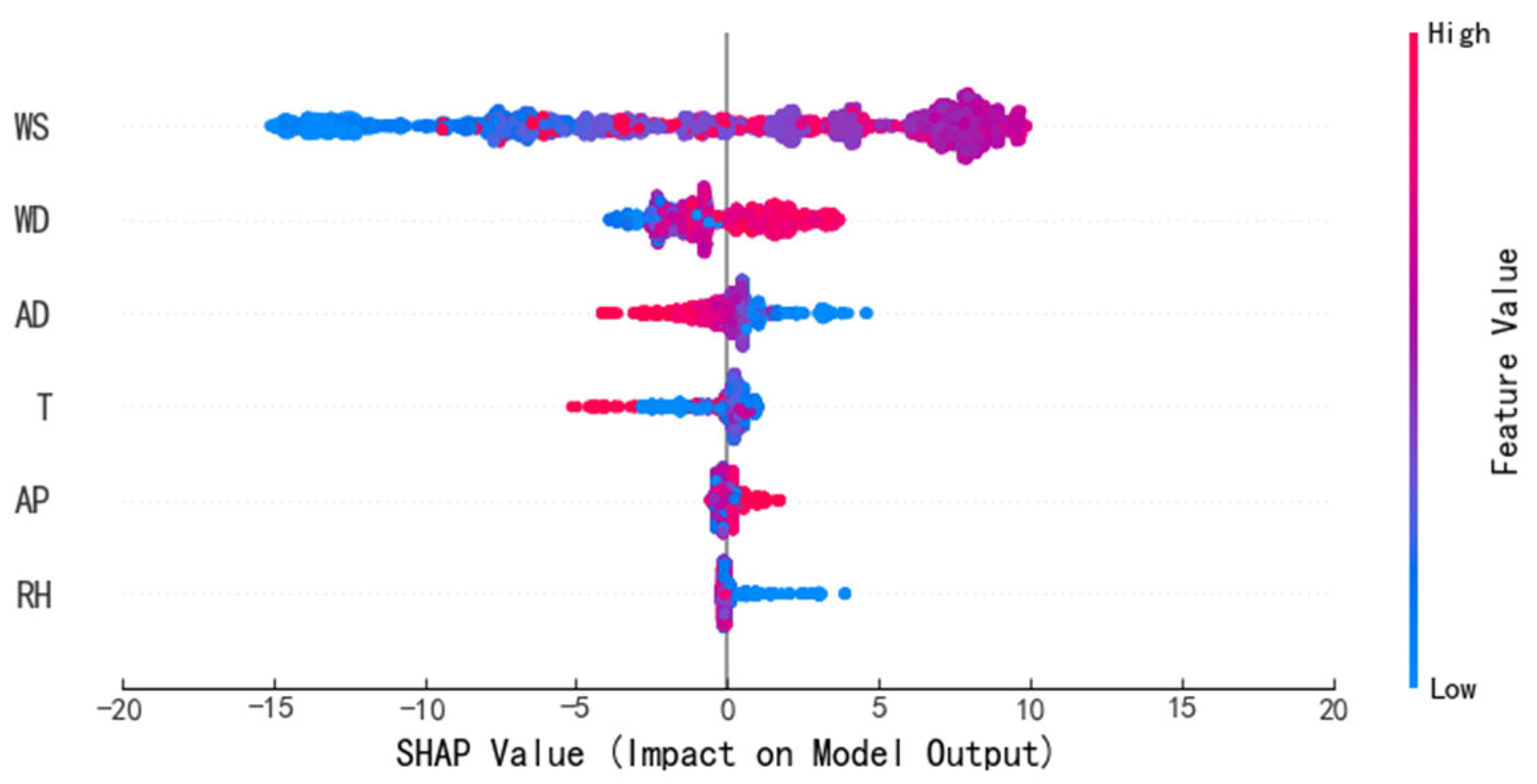
Prior to the combination experiments, Shapley additive explanations (SHAP) was applied to perform a preliminary importance analysis of six commonly used meteorological features, including wind speed (WS), wind direction (WD), temperature (T), relative humidity (RH), air density (AD), and atmospheric pressure (AP). SHAP values quantify the marginal contribution of each feature to the model output at the sample level. As shown in
Figure 3, this analysis not only provides a reference for selecting effective input features but also enhances the interpretability of the model by revealing how different variables influence its predictions. Such interpretability contributes to better transparency and increases user trust in the model’s decision-making process.
Based on the SHAP analysis, various feature combinations were constructed and evaluated using the XGBoost model. The prediction performance of each combination, measured by MAE, MSE, RMSE, and R
2, is presented in
Table 3. The results indicate that the combination of wind speed, wind direction, humidity, and temperature yields the best overall performance, achieving the lowest MAE of 7.68 and the highest R
2 of 0.44. Compared to models using only wind speed or a limited set of features, this combination demonstrates improved accuracy and stability.
In summary, SHAP provides a quantitative interpretation of the relative importance of meteorological features, which supports the design of more effective input combinations. The experimental results further validate the advantage of multi-variable input schemes in wind power prediction. Incorporating features such as wind direction, humidity, and temperature not only improves predictive accuracy but also contributes to the interpretability and practical applicability of the model while maintaining computational efficiency.
4.2. Technical Indicator Feature Importance Analysis Experiment
To evaluate the effectiveness of the constructed technical indicator features, the sample coverage method based on the XGBoost model (i.e., the Cover method) was used on Dataset 1 to calculate the contribution of each feature to the samples covered by the model’s split nodes. The importance of the features is then presented in tabular form. The Cover method measures the relationship between the number of samples covered by the feature in the split decision and the split gain, providing an intuitive reflection of the feature’s impact on the model’s prediction performance.
Table 4 presents the calculated importance scores of the features. The meteorological data used in the table corresponds to the best meteorological feature combination verified in
Section 3.1. From the feature importance scores of Groups 4 and 5 in
Table 4, it can be seen that the feature construction method proposed in this study, including technical indicators and power fluctuation indicators, has significantly higher importance than the meteorological data features. The total importance score of the meteorological data in Group 4 is only 57% of the total importance score of the technical indicators. In Group 6, when considering all features, the power technical indicator MA ranks first in feature importance, with other technical indicators also occupying important positions. This shows that, compared to meteorological data, technical indicators and power fluctuation features contribute more to the improvement of the model’s prediction performance, fully validating the effectiveness and superiority of the constructed features in wind power prediction.
4.3. Comparative Experiment
To comprehensively evaluate the predictive performance and generalization capability of the proposed MTI-XGBoost model for ultra-short-term wind power prediction, comparative experiments were conducted using two real-world datasets, as described in
Section 3.1. The evaluation employed the five metrics introduced in
Section 3.2: mean absolute error (MAE), mean squared error (MSE), root mean squared error (RMSE), the coefficient of determination (R
2), and training time. These metrics jointly assess both predictive accuracy and computational efficiency. All the models were trained and tested independently on each dataset under consistent hyperparameter settings and data partitioning strategies. Each experiment was repeated ten times, and the results are reported as means ± standard deviations to reflect model stability and robustness.
Furthermore, to determine the statistical significance of the performance differences, paired-sample t-tests were conducted to compare MTI-XGBoost with baseline models based on RMSE, with a significance level set at α = 0.05.
Table 5 summarizes the performance of all the models on Dataset 1 (a wind farm in Inner Mongolia) and Dataset 2 (ENTSO-E wind power data from Germany). As shown in the table, the MTI-XGBoost model achieved the best performance across both datasets in terms of prediction accuracy and computational efficiency. On Dataset 1, the model obtained an RMSE of 2.7049 ± 0.0036 and an R
2 of 0.9555 ± 0.0001, with a training time of just 0.1290 ± 0.0057 s. On Dataset 2, it achieved an RMSE of 0.5684 ± 0.0008 and an R
2 of 0.9932 ± 0.0001, with a training time of 0.2090 ± 0.0099 s. The results of the
t-tests confirmed that the performance improvements of MTI-XGBoost over all the baseline models were statistically significant (
p < 0.05), further validating its robustness and superiority.
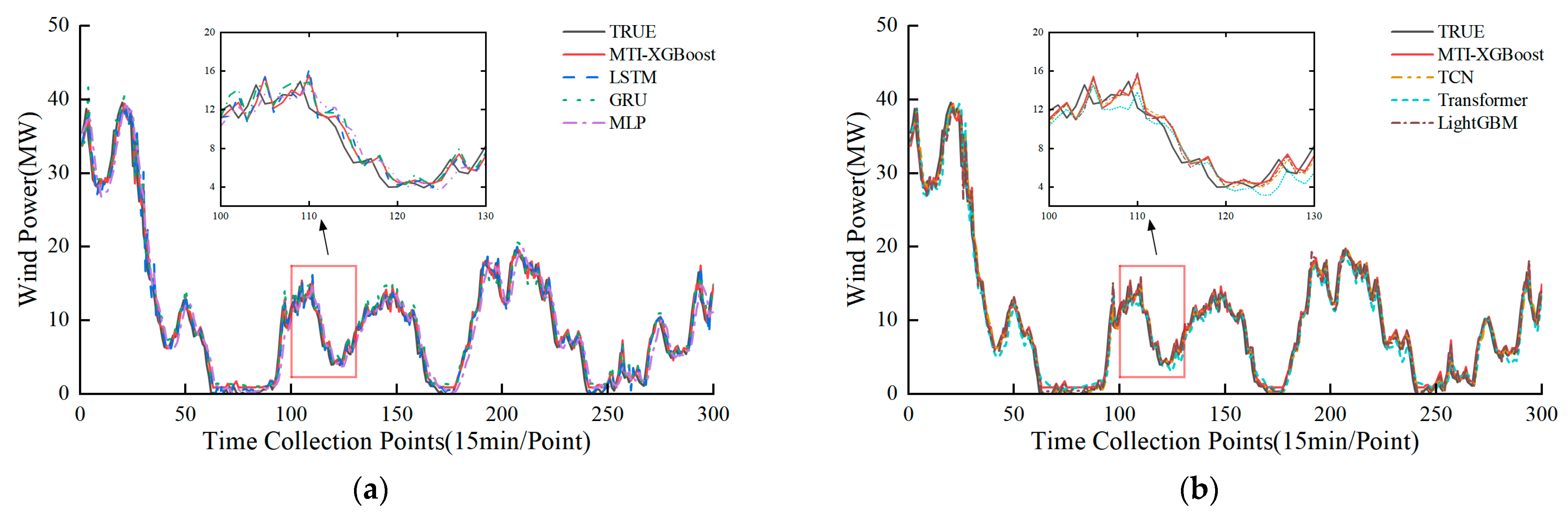
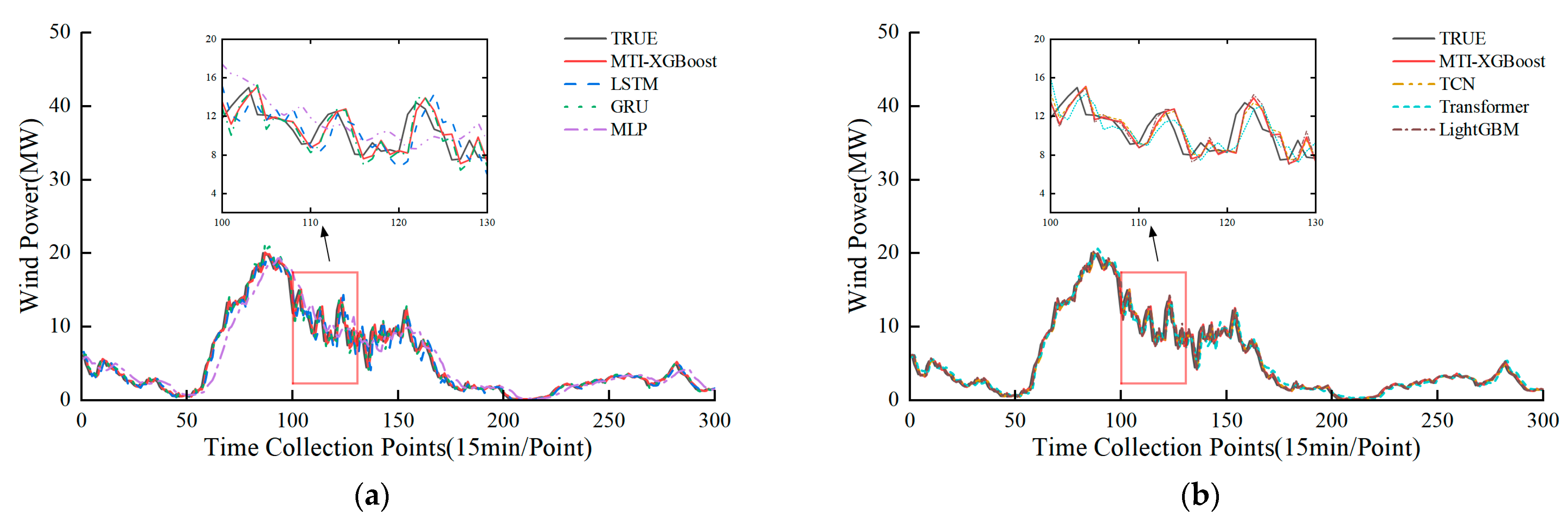
To visually demonstrate the predictive capability of the proposed model, visualization analyses were conducted on both datasets. For Dataset 1 (Inner Mongolia wind farm), the data spanned from 1 January to 11 May 2019, with a 15 min sampling interval, resulting in approximately 12,500 data points.
Figure 4 shows the predictions of MTI-XGBoost and the six benchmark models over 300 consecutive time points from the test set, including a zoomed-in segment to highlight the model’s ability to track short-term fluctuations.
For Dataset 2 (Germany ENTSO-E), the data spanned from 1 January 2015, to 5 June 2016, also with a 15 min sampling interval, yielding approximately 50,000 data points.
Figure 5 presents the predictions of all the models over 300 consecutive test points, along with a zoomed-in view to examine local variation tracking. These visualizations further demonstrate the generalization ability of MTI-XGBoost across different wind regimes and regional characteristics. All training and evaluation procedures were conducted on the full datasets with consistent experimental settings to ensure fairness and reproducibility.
In
Figure 4 and
Figure 5, the black lines represent the actual values, while the red lines denote the predictions made by MTI-XGBoost.
Figure 4 highlights the model’s precise tracking of rapid fluctuations in Dataset 1, while
Figure 5 confirms its adaptability to the ENTSO-E dataset. In both cases, the MTI-XGBoost predictions closely align with the actual values and clearly outperform all other models, demonstrating the model’s superior accuracy in ultra-short-term wind power prediction.
Taking Dataset 1 as an example (
Figure 4 and
Table 5), compared with the LSTM baseline, the proposed model achieved improvements of 5.23%, 11.38%, 5.81%, and 0.58% in MAE, MSE, RMSE, and R
2, respectively. Additionally, the training time was drastically reduced from 106 s to just 0.129 s. On Dataset 2, MTI-XGBoost similarly outperformed all benchmarks across all evaluation metrics, underscoring its strong adaptability and stability in diverse wind power scenarios. These results collectively show that the proposed machine learning approach offers not only superior predictive performance but also significantly enhanced efficiency compared to deep learning models, confirming its practical effectiveness and reliability for real-world applications.
4.4. Ablation Experiment
We aimed to validate the performance of the MTI-XGBoost model in the context of wind power prediction by conducting ablation studies, with a specific focus on the impact of individual technical indicators. All the experiments were carried out on Dataset 1 (wind farm data from Inner Mongolia). The details of the experimental setup and the corresponding results are presented in
Table 6.
Six distinct experimental configurations were established in this study. In Group 1, the model inputs consisted of numerical weather prediction variables, primarily covering meteorological parameters such as wind speed, direction, humidity, and ambient temperature. In Group 2, the input features included numerical weather prediction data and power fluctuation features, where the power fluctuation features consisted of the current power value, the previous power value, and the difference between the two. Groups 3 to 5 included power fluctuation features, numerical weather prediction data, and technical indicators as their input features. Group 6 included only power fluctuation features and technical indicators. Based on
Table 6, the following observations were made:
Group 1, which uses only numerical weather prediction data for wind power prediction, performs poorly, with MAE, MSE, RMSE, and R2 significantly lagging behind the other groups.
Group 2, which introduces power fluctuation features, shows a significant improvement in the MTI-XGBoost model’s performance. Compared to Group 1, the MSE improved by 91.51%, indicating that the inclusion of power fluctuation features significantly enhances the accuracy of wind power prediction.
Groups 3 to 5 introduce technical indicators, further improving the model’s prediction performance. Taking Group 2 as a baseline, the MSE of Groups 3, 4, and 5 improved by 3.17%, 4.31%, and 5.24%, respectively. As more technical indicators were added, the model’s prediction performance gradually improved.
Group 6 removed the numerical weather prediction data. Comparing Group 6 with Groups 2 and 5 shows that the combination of technical indicators and power fluctuation features performs better than relying solely on numerical weather prediction data. Combining all three features actually reduces prediction accuracy, indicating that the introduction of technical indicators and power fluctuation features reduces the model’s reliance on meteorological data, providing a new solution for wind power prediction.
4.5. The Role of Technical Indicators
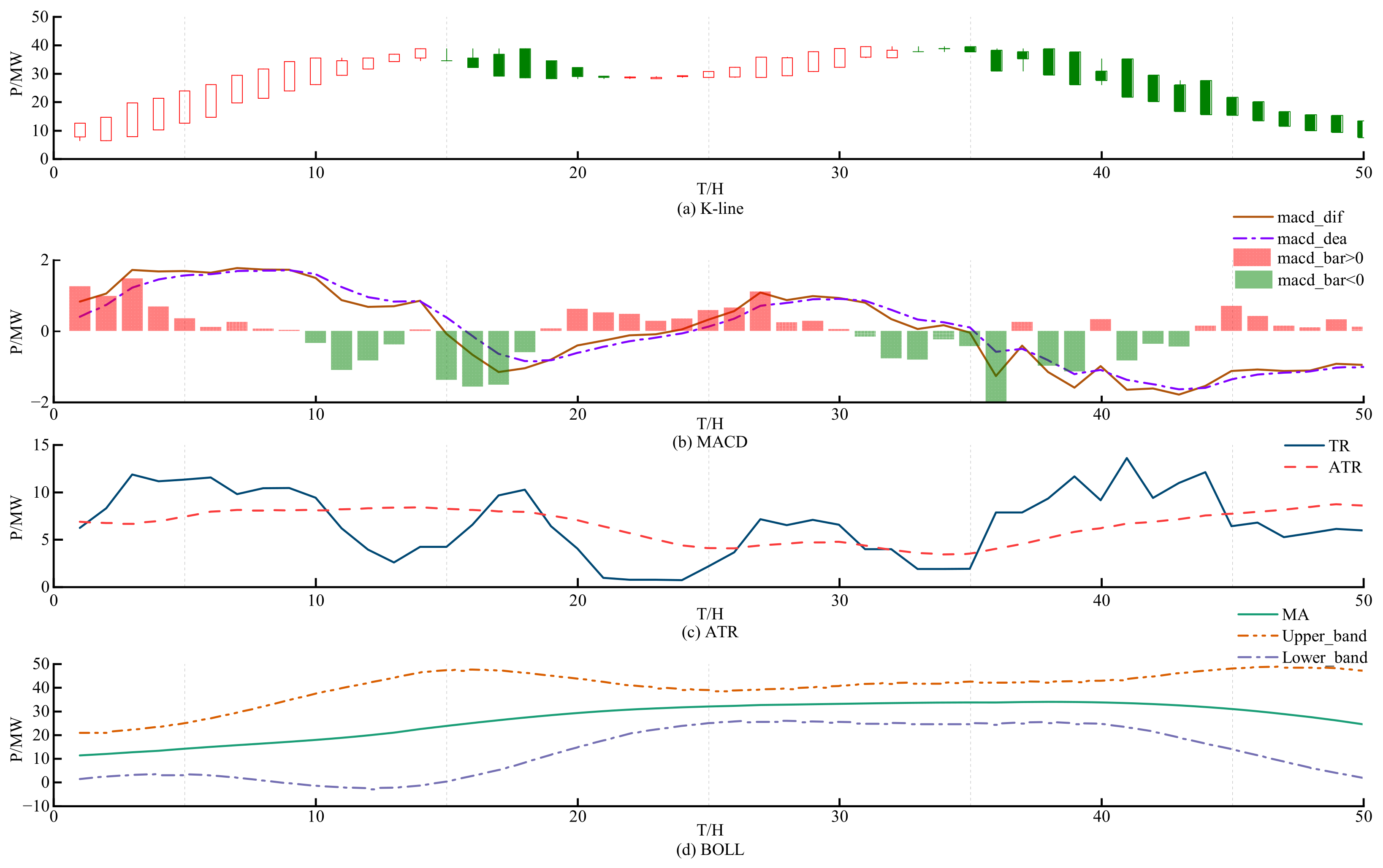
The visualization results presented in
Figure 6 are based on Dataset 1, which contains wind power data collected from a wind farm in Inner Mongolia.
The plotting results of the technical indicator MACD are shown in
Figure 6b. The solid brown line represents the DIF line, which reflects the trend of wind power fluctuations. The purple dashed line represents the DEA line, which is the moving average of the DIF line, smoothing the fluctuations of the DIF line and providing a clearer display of the wind power trend. The red and green BAR histograms represent the differences between the DIF and DEA lines: when the BAR is positive, it indicates that the DIF is above the DEA, generally corresponding to an upward trend in wind power; conversely, when the BAR is negative, it indicates a downward trend in wind power. The BAR histogram visually reflects the momentum and strength of the wind power trend, and its application in prediction helps improve model accuracy.
The plotting results of the technical indicator ATR are shown in
Figure 6c. The solid dark blue line represents the TR line, which tracks the trend of wind power fluctuations. Comparing with
Figure 6a, the TR line can anticipate the upward or downward trends of wind power. The red dashed line represents the ATR line, which is derived from the TR line and reflects the average extent of wind power fluctuations. The application of the ATR indicator improves the model’s ability to assess wind power trends, thereby increasing prediction accuracy.
The plotting results of the technical indicator BOLL are shown in
Figure 6d. The solid green line represents the MA line, which is the middle band of the Bollinger Bands, reflecting the trend of wind power fluctuations. The orange-brown dashed line represents the UB line, the upper band, showing the upper limit and pressure area of wind power; the light purple-blue dashed line represents the LB line, the lower band, indicating the lower limit and support area of wind power. The application of the BOLL indicator further enhances the model’s prediction accuracy.
This study proposes a feature engineering method combining multiple technical indicators. By integrating the three indicators and utilizing their sensitivity to wind power time series data and trend judgment capabilities, the prediction accuracy is enhanced. In the stock market, events like “black swans” and “gray rhinos” often trigger severe volatility. These events have similar impact mechanisms to wind power fluctuations, and they can unpredictably affect the market or data. Therefore, when constructing prediction models, it is crucial to fully consider these factors to enhance the model’s robustness and accuracy.
5. Conclusions
This study proposes an ultra-short-term wind power prediction method that integrates multiple technical indicators with the XGBoost model. The method was validated on two real-world datasets: Dataset 1, collected from a wind farm in Inner Mongolia, China, and Dataset 2, sourced from ENTSO-E wind power data in Germany. The experimental results demonstrate that the proposed approach exhibits excellent predictive performance, strong generalization ability across different regions and scenarios, and enhanced interpretability. The main conclusions are as follows:
By combining multiple technical indicators with the feature learning framework, the potential information in wind power time series data was effectively mined, enabling the more accurate capture of wind power fluctuation trends and significantly improving the model’s prediction accuracy.
The use of the XGBoost model greatly reduces training time, enhancing computational efficiency while maintaining high predictive accuracy. Across both datasets, the model achieved fast and reliable training and inference, making it well-suited for real-time prediction applications.
Compared to deep learning models such as LSTM, the proposed method yields comparable or superior results. For instance, on Dataset 1, the MSE was reduced by approximately 11.4% compared to the LSTM model, demonstrating that the combination of technical indicators and power fluctuation features can effectively compensate for the complexity of deep neural networks.
Overall, the proposed method overcomes the limitations of traditional feature extraction approaches, fully utilizes technical indicators to characterize wind power trends, and achieves efficient, accurate, and interpretable prediction. Thanks to the tree-based structure of XGBoost, the model provides clear explanations of feature contributions, improving transparency and fostering trust in model decisions. The approach also demonstrates strong generalization across diverse geographical and operational contexts, offering valuable support for wind power integration, dispatch, and power system operations. Future research will focus on improving outlier correction and parameter optimization to further enhance prediction stability and adaptability, promoting the transition of wind power technology from passive grid adaptation to active grid support.


