Determining Pilot Ignition Delay in Dual-Fuel Medium-Speed Marine Engines Using Methanol or Hydrogen

Abstract

Dual-fuel engines are a way of transitioning the marine sector to carbon-neutral fuels like hydrogen and methanol. For the development of these engines, accurate simulation of the combustion process is needed, for which calculating the pilot’s ignition delay is essential. The present work investigates novel methodologies for calculating this. This involves the use of chemical kinetic schemes to compute the ignition delay for various operating conditions. Machine learning techniques are used to train models on these data sets. A neural network model is then implemented in a dual-fuel combustion model to calculate the ignition delay time and is compared using a lookup table or a correlation. The numerical results are compared with experimental data from a dual-fuel medium-speed marine engine operating with hydrogen or methanol, from which the method with best accuracy and fastest calculation is selected.

1. Introduction

Maritime transport contributed nearly 3% of global anthropogenic ${\mathrm{C}\mathrm{O}}_2$ emissions in 2018 [1]. Within the EU, shipping industry accounted for an estimated 3 to 4% of total emissions, producing over 144 million tons of ${\mathrm{C}\mathrm{O}}_2$ in 2019 [2]. The maritime sector is expected to grow by between 25% and 180% by 2050 [2]. Projections indicate that that the carbon emissions caused by maritime transport could rise by up to 130% compared to 2008 levels by 2050. In response, the European Union has mandated reductions of 2% by 2025 and 80% by 2050 [1,3,4]. Therefore, urgent actions should be taken to meet the targets.

One of the promising ways to achieve these emission reduction targets is to transition to renewable fuels like hydrogen and methanol [5,6]. Gaseous hydrogen, as a clean energy carrier, is highly regarded as a promising fuel for the future, as it can be sourced from renewable source [7,8]. For marine applications, it is expected to be used where it outperforms the energy density of batteries, but where autonomy demands are still limited. If these demands become stricter, a denser energy carrier is needed, for which several hydrogen carriers are being considered. One of these is methanol [5,9,10]. Being liquid under ambient conditions, methanol facilitates easy handling and transportation; furthermore it is relatively straightforward to produce from biomass feedstocks and renewable electricity [11,12].

Hydrogen and methanol can serve as primary fuels in internal combustion engines (ICE). However, in compression ignition (CI) engines, the prime power plant for marine transportation, they cannot be used as such, due to their high autoignition temperature (reflected in their high octane numbers). A way around this is to use a pilot injection of a diesel-like fuel with low autoignition temperature (high cetane number), which then initiates combustion. Thus, methanol and hydrogen can be used in a dual-fuel mode. Hydrogen has a wide flammability range and fast flame speed, which makes it a promising solution for managing challenges associated with other gaseous fuels. Its application in dual-fuel diesel engines can improve thermal efficiency due to its faster flame velocity than other gaseous fuels [13]. Additionally, hydrogen does not contain structural carbon; it could thus reduce emissions of unburned hydrocarbons ($\mathrm{U}\mathrm{H}\mathrm{C}$) and carbon monoxide ($\mathrm{C}\mathrm{O}$) in dual-fuel engines [7,14]. Methanol also demonstrates excellent engine performance with high efficiency and extremely low emissions compared to hydrocarbons such as petrol and diesel fuels [5,15,16], with its low flame temperatures leading to reduction in oxides of nitrogen (${\mathrm{N}\mathrm{O}}_{\mathrm{x}}$) and with no soot formation due to its carbon atom being bonded to an oxygen atom.

Various approaches are available for dual-fuel engines, primarily determined by the way hydrogen or methanol is injected into the engine. One of these methods is direct injection into the cylinder alongside a burning diesel jet [17,18], or they can be fumigated into the intake manifold at a single point or multiple points before reaching the intake valves [19,20]. In this study, port fuel injection (PFI) is focused on because it offers the most convenient solution for retrofitting engines. This is particularly important for the marine sector as the average age of vessels is over 20 years so one cannot solely rely on newbuilds to reduce the carbon emissions. The PFI method benefits from a low-pressure (and thus low cost) fuel circuit and requires very few engine modifications because methanol or hydrogen are introduced into the intake manifold [19,21]. This fumigation concept has been extensively studied and demonstrated over the past decade, but challenges persist. Hydrogen poses significant challenges with PFI, including issues like pre-ignition, knock, and backfiring due to its wide flammability range, low minimum ignition energy, and limited quenching distance. Furthermore, hydrogen displaces air in the intake, limiting the engine’s power density [22]. For methanol, its high heat of vaporization can lead to potentially severe diesel knock under high load conditions [23]. The strong cooling caused by this high heat of evaporation also complicates ignition during cold starts, warming up, and low-load conditions [24,25]. Additionally, there is an increase in the levels of $\mathrm{C}\mathrm{O}$ and $\mathrm{T}\mathrm{H}\mathrm{C}$ [26] due to the fuel being premixed and thus entering combustion chamber crevices where a flame cannot propagate.

Conventional high-performance diesel engines normally have high valve overlap to ensure that residual gases are completely evacuated from the cylinder. Converting these engines to PFI dual-fuel operation introduces some challenges [27]. In methanol–diesel dual-fuel engines, some of the methanol–air mixture may escape into the exhaust during the valve overlap period, a phenomenon known as scavenging loss. This unburned fuel loss results in two main issues: first, it negatively impacts the engine’s thermal efficiency; second, it leads to an increase in unburned methanol emissions. Zhenyu Sun et al. [27] found that valve timing affects methanol film formation and fuel scavenging losses. Therefore, it can significantly reduce thermal efficiency. They concluded that during the valve overlap period, unburned methanol escapes into the exhaust, resulting in reduced combustion efficiency. In hydrogen/diesel engines, hydrogen’s low ignition energy and high diffusivity increase the risk of backfiring or early ignition during valve overlap. Studies show that high valve overlap makes this issue worse, but optimizing injection timing and valve overlap can help reduce the risk [28].

A comprehensive understanding of hydrogen/diesel and methanol/diesel co-combustion is vital to effectively addressing these challenges. One of the critical parameters for accurately simulating PFI dual-fuel combustion of hydrogen/diesel and methanol/diesel is the pilot ignition delay—the time between the start of pilot injection and the start of pilot combustion—as diesel is now injected into an air–fuel mixture with properties different from air. The results reported by Dierickx et al. [19], shown in Figure 1, illustrate how increasing the methanol energy fraction (MEF) significantly influences the ignition delay time of diesel in a PFI dual-fuel engine. As MEF increases, the start of combustion, shown by an increase in the pressure rise rate (marked with a red circle), occurs later in the cycle. This shift clearly reflects a longer ignition delay associated with higher levels of methanol substitution. If this time is incorrectly estimated, the whole combustion process will be calculated wrongly. Few studies have looked into how to calculate the ignition delay time in PFI dual-fuel engines operating on hydrogen or methanol under actual engine conditions.

In dual-fuel operation using hydrogen, there is no evaporative cooling, which influences the intake air temperature since hydrogen is usually introduced as a gas. Hydrogen’s heat capacity at standard temperature (20 °C) and pressure (1 atm) is approximately 14 times greater than that of air, specifically 14.28 kJ/(kg K). This increased heat capacity of the mixture results in smaller rise in temperature while compressing [29,30]. Additionally, when hydrogen is added into the port, it displaces some of the intake air due to its low density, which reduces the volumetric efficiency compared to diesel operation and consequently lowers reduces the amount of oxygen in the intake mixture [28,31]. All these factors influence the temperature and the oxygen availability during diesel injection, affecting the ignition delay [30]. The chemical influence of premixed hydrogen or methanol on the ignition delay of a diesel pilot was investigated by Parsa et al. [32]. They concluded that premixed hydrogen did not notably impact the ignition delay of the pilot fuel, except when the percentage of hydrogen in the premixed fuel was significantly high. However, the ignition delay of the pilot fuel is greatly influenced by the presence of premixed methanol.

Introducing methanol into the incoming air in dual-fuel applications has been reported to prolong the ignition delay of the diesel pilot. This delay results from several elements. Firstly, methanol’s high heat of vaporization [5,20] lowers the temperature of the intake air-fuel mix significantly, which reduces the temperature and pressure at the moment when diesel fuel starts being injected [19,33]. In addition, the higher heat capacity of the intake mixture also limits the rise in temperature as the mixture is compressed [33]. Additionally, Yin et al. [34] found that at a methanol-to-air equivalence ratio of 0.1 and temperatures under 920 K, methanol slows down the initial chemical reaction rate of diesel autoignition. This effect has been linked to the temperature dependence of radical species conversion, particularly involving $\mathrm{O}\mathrm{H}·$ and ${\mathrm{H}}_2{\mathrm{O}}_2$.

Few studies have analyzed the ignition delay of hydrogen/diesel and methanol/diesel dual-fuel engines under actual engine operation scenarios. Dhole et al. [35] conducted an experimental study on the combustion duration and ignition delay of a dual-fuel diesel engine using hydrogen, producer gas, and various mixtures of producer gas and hydrogen as secondary fuels with a diesel pilot. The experiments were performed on a 4-cylinder turbocharged and intercooled 62.5 kW generator set diesel engine at a constant speed of 1500 rpm. Their findings indicated that at low loads, replacing 30% (mass percentage) of the diesel fuel with hydrogen extended the combustion duration by 2.5 crank angle degrees (CA) and lengthened the ignition delay by 2° CA. However, at higher loads (80%) with 50% hydrogen substitution (mass percentage), both the ignition delay and combustion duration were reduced. The study also found that the ignition delay in dual-fuel engines is influenced not only by the type and concentration of gaseous fuels but also by the charge temperature, pressure, and oxygen content.

Some correlations have been proposed for estimating the ignition delay of methanol/diesel and hydrogen/diesel dual-fuel combustion. Dierickx et al. [36] proposed a correlation for the calculation of ignition delays in dual-fuel engines with hydrogen or methanol in a medium speed single cylinder engine. The newly developed methanol dual-fuel correlation incorporates the inhibition effect using the methanol-air equivalence ratio. Consequently, the ignition delay increases with a rising methanol-air equivalence ratio, resulting from an increased methanol content in the cylinder, besides temperature, pressure, and diesel equivalence ratio effects. In dual-fuel operation with hydrogen, this study discovered that the measured ignition delay was minimally affected by increasing the hydrogen energy fraction. However, they observed that ignition delay slightly decreased when they analyzed the temperature and pressure changes during the ignition delay and their impact on the various elements of the ignition delay correlations. Zong et al. [37] integrated a skeletal kinetic model developed by Xu et al. [38] for predicting the ignition delay of methanol/n-heptane into a diesel-methanol dual-fuel 3D CFD study. Also, Decan et al. [39] used tabulated ignition delays estimated by detailed chemistry schemes in the CFD simulation of a fumigated dual-fuel engine.

According to the literature review, an accurate estimation of the ignition delay in dual-fuel engines operating on hydrogen or methanol is necessary for any simulation of dual-fuel combustion, and it should be applicable as generally as possible. As discussed above, the ignition delay can be calculated in different ways: either through a correlation that typically incorporates some physics but is mostly phenomenological in nature, i.e., fitted to experimental data; or through chemical kinetic simulations. The latter are the best starting point, as they do not depend on engine-specific data. However, these require the selection of appropriate reaction mechanisms, that properly take the effects of both premixed fuel and pilot fuel into account. Also, as calculating the ignition delay time from chemical kinetics “on the fly”, i.e., during engine combustion simulations, is computationally expensive, these mechanisms are typically used to generate a table beforehand, covering all conditions expected in engines. There are then various options on how to use this table during engine combustion simulations. It can be used to look up the relevant ignition delay time during engine combustion simulation, but with the recent improvements in machine learning, it could also be worthwhile to use machine learning to capture the table data in a mathematical formulation. Such an approach could potentially speed up the engine calculations as less time is needed for data retrieval.

To address these research gaps, the present study thus integrates ignition delay data from chemical kinetic mechanisms, calculated using Cantera over a wide range of operating conditions, into a dual-fuel multi-zone combustion model using two different methodologies: machine learning and look-up tables, and also compares these to the results when using the correlation from Dierickx et al. [36]. The accuracy of these methodologies is then evaluated against experimental data from a medium-speed marine engine. While traditional correlations require calibration based on engine specifications to yield accurate results, it is evaluated whether the methodologies proposed in this work allow using the calculated ignition delay times without the need for any pre-calibration. Additionally, as the data are derived from chemical kinetics, the chemical effect of the premixed fuel on the ignition delay of the pilot diesel can be further elaborated.

The main long-term objective of this work is to develop a more accurate 0D/1D dual-fuel combustion model (for which GT-Power V2023 serves as the simulation environment), serving as a virtual engine for future real engine development. Accurate prediction of ignition delay time is a critical step toward achieving full-cycle simulation accuracy. This study focuses specifically on improving the start of combustion by comparing ignition delay times predicted by different methodologies against experimental engine data under various operating conditions. While the start of combustion is crucial, accurately simulating it alone does not ensure improvements across the full combustion cycle. Other factors, such as laminar and turbulent burning velocities and flame surface area, also significantly impact the combustion process. However, this study focuses completely on establishing an accurate methodology for ignition delay time prediction, without attempting full combustion cycle evaluation, which will be tackled in follow-up work.

In the following sections, a brief explanation of the experimental setup used to collect the data and the study cases examined in this work will be provided. This will be followed by a detailed explanation of the numerical methodologies, and then the results and conclusions will be presented.

2. Experimental Setup

In the present study, data measured from the single-cylinder engine (SCE) shown in Figure 2 are utilized. The engine specifications can be found in

Table 1. The engine specifications.

Engine Model Name	FM24
Cylinders	1
Compression ratio	12.1:1
Bore × stroke	240 × 290 mm (SCE1) 256 × 290 mm (SCE2)
Displacement volume	13.1 l (SCE1) and 14.9 l (SCE2)
Diesel injection system	Cam-driven Single Injection Pumps
Nominal power	200 kW (SCE1), 224 kW (SCE2)
Nominal speed	1000 rpm

. The SCE, developed in collaboration with Anglo Belgian Corporation, is located at the WTZ Roßlau laboratory. The experimental data was obtained from two different bore sizes: one with a bore size of 240 mm (SCE 1) and the other with a bore size of 256 mm (SCE 2).

In the single-cylinder engine, methanol was injected at a low pressure (below 1 MPa) into the intake port, whereas hydrogen injection was at a constant pressure, 0.05 MPa higher than the intake air pressure. The intake air temperature and pressure adjustment were based on the fuel and engine settings, as outlined in

Table 2. Experimental cases ($\mathrm{M}\mathrm{E}\mathrm{F}$ and $\mathrm{H}\mathrm{E}\mathrm{F}$ represent methanol energy fraction and hydrogen energy fraction, respectively [36]).

Campaign	Samples	Parameter Variations
MEOH-SCE1	1	${\mathrm{P}}_{\mathrm{a}\mathrm{i}\mathrm{r}}=0.35 \mathrm{M}\mathrm{P}\mathrm{a},{\mathrm{T}}_{\mathrm{a}\mathrm{i}\mathrm{r}}=324.15 \mathrm{K},\hspace{1em}\hspace{1em}\mathrm{M}\mathrm{E}\mathrm{F}=60\mathrm{\%},\hspace{1em}\hspace{1em}\mathrm{l}\mathrm{o}\mathrm{a}\mathrm{d}=75\mathrm{\%}$
	2, 3	${\mathrm{P}}_{\mathrm{a}\mathrm{i}\mathrm{r}}=0.35 \mathrm{M}\mathrm{P}\mathrm{a},{\mathrm{T}}_{\mathrm{a}\mathrm{i}\mathrm{r}}=348.15 \mathrm{K},\hspace{1em}\hspace{1em}\mathrm{M}\mathrm{E}\mathrm{F}=60, 70\mathrm{\%},\hspace{1em}\hspace{1em}\mathrm{l}\mathrm{o}\mathrm{a}\mathrm{d}=75\mathrm{\%}$
	4, 5	${\mathrm{P}}_{\mathrm{a}\mathrm{i}\mathrm{r}}=0.35 \mathrm{M}\mathrm{P}\mathrm{a},{\mathrm{T}}_{\mathrm{a}\mathrm{i}\mathrm{r}}=358.15 \mathrm{K},\hspace{1em}\hspace{1em}\mathrm{M}\mathrm{E}\mathrm{F}=70, 73\mathrm{\%},\hspace{1em}\hspace{1em}\mathrm{l}\mathrm{o}\mathrm{a}\mathrm{d}=75\mathrm{\%}$
	6, 7	${\mathrm{P}}_{\mathrm{a}\mathrm{i}\mathrm{r}}=0.35 \mathrm{M}\mathrm{P}\mathrm{a},{\mathrm{T}}_{\mathrm{a}\mathrm{i}\mathrm{r}}=324.15 \mathrm{K},\hspace{1em}\hspace{1em}\mathrm{M}\mathrm{E}\mathrm{F}=50, 60\mathrm{\%},\hspace{1em}\hspace{1em}\mathrm{l}\mathrm{o}\mathrm{a}\mathrm{d}=75\mathrm{\%}$
	8, 9	${\mathrm{P}}_{\mathrm{a}\mathrm{i}\mathrm{r}}=3.5 \mathrm{M}\mathrm{P}\mathrm{a},{\mathrm{T}}_{\mathrm{a}\mathrm{i}\mathrm{r}}=348.15 \mathrm{K},\hspace{1em}\hspace{1em}\mathrm{M}\mathrm{E}\mathrm{F}=50, 60\mathrm{\%},\hspace{1em}\hspace{1em}\mathrm{l}\mathrm{o}\mathrm{a}\mathrm{d}=75\mathrm{\%}$
	10, 11	${\mathrm{P}}_{\mathrm{a}\mathrm{i}\mathrm{r}}=0.33 \mathrm{M}\mathrm{P}\mathrm{a},{\mathrm{T}}_{\mathrm{a}\mathrm{i}\mathrm{r}}=324.15 \mathrm{K},\hspace{1em}\hspace{1em}\mathrm{M}\mathrm{E}\mathrm{F}=50, 60\mathrm{\%},\hspace{1em}\hspace{1em}\mathrm{l}\mathrm{o}\mathrm{a}\mathrm{d}=75\mathrm{\%}$
	12, 13	${\mathrm{P}}_{\mathrm{a}\mathrm{i}\mathrm{r}}=0.35 \mathrm{M}\mathrm{P}\mathrm{a},{\mathrm{T}}_{\mathrm{a}\mathrm{i}\mathrm{r}}=324.15 \mathrm{K},\hspace{1em}\hspace{1em}\mathrm{M}\mathrm{E}\mathrm{F}=50, 60\mathrm{\%},\hspace{1em}\hspace{1em}\mathrm{l}\mathrm{o}\mathrm{a}\mathrm{d}=75\mathrm{\%}$
	14, 15	${\mathrm{P}}_{\mathrm{a}\mathrm{i}\mathrm{r}}=0.37 \mathrm{M}\mathrm{P}\mathrm{a},{\mathrm{T}}_{\mathrm{a}\mathrm{i}\mathrm{r}}=324.15 \mathrm{K},\hspace{1em}\hspace{1em}\mathrm{M}\mathrm{E}\mathrm{F}=50, 60\mathrm{\%},\hspace{1em}\hspace{1em}\mathrm{l}\mathrm{o}\mathrm{a}\mathrm{d}=75\mathrm{\%}$
MEOH-SCE2	1	${\mathrm{P}}_{\mathrm{a}\mathrm{i}\mathrm{r}}=0.37 \mathrm{M}\mathrm{P}\mathrm{a},{\mathrm{T}}_{\mathrm{a}\mathrm{i}\mathrm{r}}=324.15 \mathrm{K},\hspace{1em}\hspace{1em}\mathrm{M}\mathrm{E}\mathrm{F}=46, 51\mathrm{\%},\hspace{1em}\hspace{1em}\mathrm{l}\mathrm{o}\mathrm{a}\mathrm{d}=75\mathrm{\%}$
	2	${\mathrm{P}}_{\mathrm{a}\mathrm{i}\mathrm{r}}=0.36 \mathrm{M}\mathrm{P}\mathrm{a},{\mathrm{T}}_{\mathrm{a}\mathrm{i}\mathrm{r}}=358.15 \mathrm{K},\hspace{1em}\hspace{1em}\mathrm{M}\mathrm{E}\mathrm{F}=50\mathrm{\%},\hspace{1em}\hspace{1em}\mathrm{l}\mathrm{o}\mathrm{a}\mathrm{d}=75\mathrm{\%}$
	3	${\mathrm{P}}_{\mathrm{a}\mathrm{i}\mathrm{r}}=0.36 \mathrm{M}\mathrm{P}\mathrm{a},{\mathrm{T}}_{\mathrm{a}\mathrm{i}\mathrm{r}}=348.15 \mathrm{K},\hspace{1em}\hspace{1em}\mathrm{M}\mathrm{E}\mathrm{F}=50\mathrm{\%},\hspace{1em}\hspace{1em}\mathrm{l}\mathrm{o}\mathrm{a}\mathrm{d}=75\mathrm{\%}$
	4	${\mathrm{P}}_{\mathrm{a}\mathrm{i}\mathrm{r}}=0.31 \mathrm{M}\mathrm{P}\mathrm{a},{\mathrm{T}}_{\mathrm{a}\mathrm{i}\mathrm{r}}=348.15 \mathrm{K},\hspace{1em}\hspace{1em}\mathrm{M}\mathrm{E}\mathrm{F}=45\mathrm{\%},\hspace{1em}\hspace{1em}\mathrm{l}\mathrm{o}\mathrm{a}\mathrm{d}=75\mathrm{\%}$
	5	${\mathrm{P}}_{\mathrm{a}\mathrm{i}\mathrm{r}}=0.36 \mathrm{M}\mathrm{P}\mathrm{a},{\mathrm{T}}_{\mathrm{a}\mathrm{i}\mathrm{r}}=348.15 \mathrm{K},\hspace{1em}\hspace{1em}\mathrm{M}\mathrm{E}\mathrm{F}=51\mathrm{\%},\hspace{1em}\hspace{1em}\mathrm{l}\mathrm{o}\mathrm{a}\mathrm{d}=75\mathrm{\%}$
	6–8	${\mathrm{P}}_{\mathrm{a}\mathrm{i}\mathrm{r}}=0.19 \mathrm{M}\mathrm{P}\mathrm{a},{\mathrm{T}}_{\mathrm{a}\mathrm{i}\mathrm{r}}=348.15 \mathrm{K},\hspace{1em}\hspace{1em}\mathrm{M}\mathrm{E}\mathrm{F}=50, 56 ,61\mathrm{\%},\hspace{1em}\hspace{1em}\mathrm{l}\mathrm{o}\mathrm{a}\mathrm{d}=75\mathrm{\%}$
	9, 10	${\mathrm{P}}_{\mathrm{a}\mathrm{i}\mathrm{r}}=0.27 \mathrm{M}\mathrm{P}\mathrm{a},{\mathrm{T}}_{\mathrm{a}\mathrm{i}\mathrm{r}}=348.15 \mathrm{K},\hspace{1em}\hspace{1em}\mathrm{M}\mathrm{E}\mathrm{F}=50, 56\mathrm{\%},\hspace{1em}\hspace{1em}\mathrm{l}\mathrm{o}\mathrm{a}\mathrm{d}=75\mathrm{\%}$
H2-SCE1	1, 2	${\mathrm{P}}_{\mathrm{a}\mathrm{i}\mathrm{r}}=0.21 \mathrm{M}\mathrm{P}\mathrm{a},{\mathrm{T}}_{\mathrm{a}\mathrm{i}\mathrm{r}}=309.15 \mathrm{K},\hspace{1em}\hspace{1em}\mathrm{H}\mathrm{E}\mathrm{F}=25, 40\mathrm{\%},\hspace{1em}\hspace{1em}\mathrm{l}\mathrm{o}\mathrm{a}\mathrm{d}=75\mathrm{\%}$
	3, 4	${\mathrm{P}}_{\mathrm{a}\mathrm{i}\mathrm{r}}=0.21 \mathrm{M}\mathrm{P}\mathrm{a},{\mathrm{T}}_{\mathrm{a}\mathrm{i}\mathrm{r}}=316.15 \mathrm{K},\hspace{1em}\hspace{1em}\mathrm{H}\mathrm{E}\mathrm{F}=25, 40\mathrm{\%},\hspace{1em}\hspace{1em}\mathrm{l}\mathrm{o}\mathrm{a}\mathrm{d}=75\mathrm{\%}$
	5–8	${\mathrm{P}}_{\mathrm{a}\mathrm{i}\mathrm{r}}=0.2 \mathrm{M}\mathrm{P}\mathrm{a},{\mathrm{T}}_{\mathrm{a}\mathrm{i}\mathrm{r}}=316.15 \mathrm{K},\hspace{1em}\hspace{1em}\mathrm{H}\mathrm{E}\mathrm{F}=\mathrm{25,35}, \mathrm{40,44}\mathrm{\%},\hspace{1em}\hspace{1em}\mathrm{l}\mathrm{o}\mathrm{a}\mathrm{d}=75\mathrm{\%}$
	9, 10	${\mathrm{P}}_{\mathrm{a}\mathrm{i}\mathrm{r}}=0.22 \mathrm{M}\mathrm{P}\mathrm{a},{\mathrm{T}}_{\mathrm{a}\mathrm{i}\mathrm{r}}=316.15 \mathrm{K},\hspace{1em}\hspace{1em}\mathrm{H}\mathrm{E}\mathrm{F}=25, 40\mathrm{\%},\hspace{1em}\hspace{1em}\mathrm{l}\mathrm{o}\mathrm{a}\mathrm{d}=75\mathrm{\%}$
	11–13	${\mathrm{P}}_{\mathrm{a}\mathrm{i}\mathrm{r}}=0.25 \mathrm{M}\mathrm{P}\mathrm{a},{\mathrm{T}}_{\mathrm{a}\mathrm{i}\mathrm{r}}=316.15 \mathrm{K},\hspace{1em}\hspace{1em}\mathrm{H}\mathrm{E}\mathrm{F}=25, 40, 50\mathrm{\%},\hspace{1em}\hspace{1em}\mathrm{l}\mathrm{o}\mathrm{a}\mathrm{d}=75\mathrm{\%}$
	14–16	${\mathrm{P}}_{\mathrm{a}\mathrm{i}\mathrm{r}}= 0.26\mathrm{M}\mathrm{P}\mathrm{a},{\mathrm{T}}_{\mathrm{a}\mathrm{i}\mathrm{r}}=316.15 \mathrm{K},\hspace{1em}\hspace{1em}\mathrm{H}\mathrm{E}\mathrm{F}=25, 40, 50\mathrm{\%},\hspace{1em}\hspace{1em}\mathrm{l}\mathrm{o}\mathrm{a}\mathrm{d}=75\mathrm{\%}$

. An air intercooler positioned after the compressor, which controls the intake air pressure, regulates the intake air temperature. An intake air heater was employed to make final adjustments. The in-cylinder pressure sensor had a resolution of 1 crank angle degree. A pressure sensor was also used in the diesel high-pressure line of the pump-line-nozzle system. Both SCE1 and SCE2 are equipped with a single diesel injector that supplies diesel energy in both diesel and dual-fuel operations. The maximum diesel injection pressure is 100 MPa. Table 2 presents the different experimental cases whose data are used in this study. More details about the experimental setup and the cases can be found in the literature [36].

3. Numerical Methodology

As mentioned previously, this study employs various methods to estimate the ignition delay time in dual-fuel marine engines. Initially, a constant volume batch reactor within the open-source Cantera code is used to calculate the ignition delay time of hydrogen/n-heptane and methanol/n-heptane mixtures under different operating conditions. Once the dataset is created, machine learning techniques including Artificial Neural Network (ANN) and Support Vector Regression (SVR) are applied in MATLAB R2023a to train the models. The trained neural network is then integrated into the multi-zone combustion model in GT-Power, a commercial 0D/1D engine simulation software. As an alternative method, the data from Cantera is also implemented as a lookup table within GT-Power. The following sections explain the methodologies in more detail.

3.1. Dataset Generation Using Chemical Kinetic Mechanisms and Cantera

First, the chemical kinetic mechanisms developed by Andrae et al. [40] and Liu et al. [41] are used in Cantera under various operating conditions to generate the datasets for methanol/diesel and hydrogen/diesel, respectively. It is worth mentioning that the ignition delay time is defined as the time at which the OH species concentration peaks. Four input parameters are considered: pressure (P), temperature (T), the overall equivalence ratio (φ), and the molar percentage of methanol or hydrogen in the mixture.

Table 3. Data range used for training.

	P (MPa)	T (K)	φ	Molar Percentage	Number of Datapoints
Methanol/diesel	7–13	625–1800	0.5–3.5	0–95	5240
Hydrogen/diesel	4–10	625–1100	0.5–3.0	0–95	3485

shows the range of input data and the number of data points used for methanol/diesel and hydrogen/diesel blends.

In the following section, two machine learning methods employed in this work are explained in more detail.

3.2. Machine Learning Method

In the present work, two different methods, namely Artificial Neural Network (ANN) and Support Vector Regression (SVR), are introduced and used to train models on the ignition delay data generated as discussed in the previous section. This is done in MATLAB. These two different methods are then compared to determine which one performs better in predicting the targets.

Before the training starts, it is important to preprocess the inputs. Four types of inputs are used: pressure (P), temperature (T), overall equivalence ratio (φ), and methanol or hydrogen molar percentage in total fuel mass. Each input must be normalized separately to prevent any single feature from dominating due to its scale, thereby improving the algorithm’s performance. Normalization also facilitates faster convergence during the training process, especially in neural networks. In this study, the “$\mathrm{m}\mathrm{a}\mathrm{p}\mathrm{m}\mathrm{i}\mathrm{n}\mathrm{m}\mathrm{a}\mathrm{x}$” method, defined by Equation (1), is employed to normalize input data. This technique, commonly used in the preprocessing stages of machine learning and neural networks, ensures equal contribution of all features to the training process and typically scales the data between −1 and 1 or 0 and 1 [42].

$${\mathrm{y}}_{\mathrm{n}}={\displaystyle \frac{\left({\mathrm{y}}_{\mathrm{m}\mathrm{a}\mathrm{x}}-{\mathrm{y}}_{\mathrm{m}\mathrm{i}\mathrm{n}}\right)({\mathrm{x}}_{\mathrm{i}}-{\mathrm{x}}_{\mathrm{m}\mathrm{i}\mathrm{n}})}{({\mathrm{x}}_{\mathrm{m}\mathrm{a}\mathrm{x}}-{\mathrm{x}}_{\mathrm{m}\mathrm{i}\mathrm{n}})}}+{\mathrm{y}}_{\mathrm{m}\mathrm{i}\mathrm{n}}\hspace{1em}\hspace{1em}{\mathrm{y}}_{\mathrm{m}\mathrm{a}\mathrm{x}}=1,\hspace{1em}\hspace{1em}{\mathrm{y}}_{\mathrm{m}\mathrm{i}\mathrm{n}}=-1$$

(1)

Here, ${\mathrm{x}}_{\mathrm{m}\mathrm{a}\mathrm{x}}$ and ${\mathrm{x}}_{\mathrm{m}\mathrm{i}\mathrm{n}}$ represent the maximum and minimum values of the actual data, respectively, while ${\mathrm{y}}_{\mathrm{n}}$ shows the normalized parameter. ${\mathrm{x}}_{\mathrm{i}}$ is the actual data to be scaled.

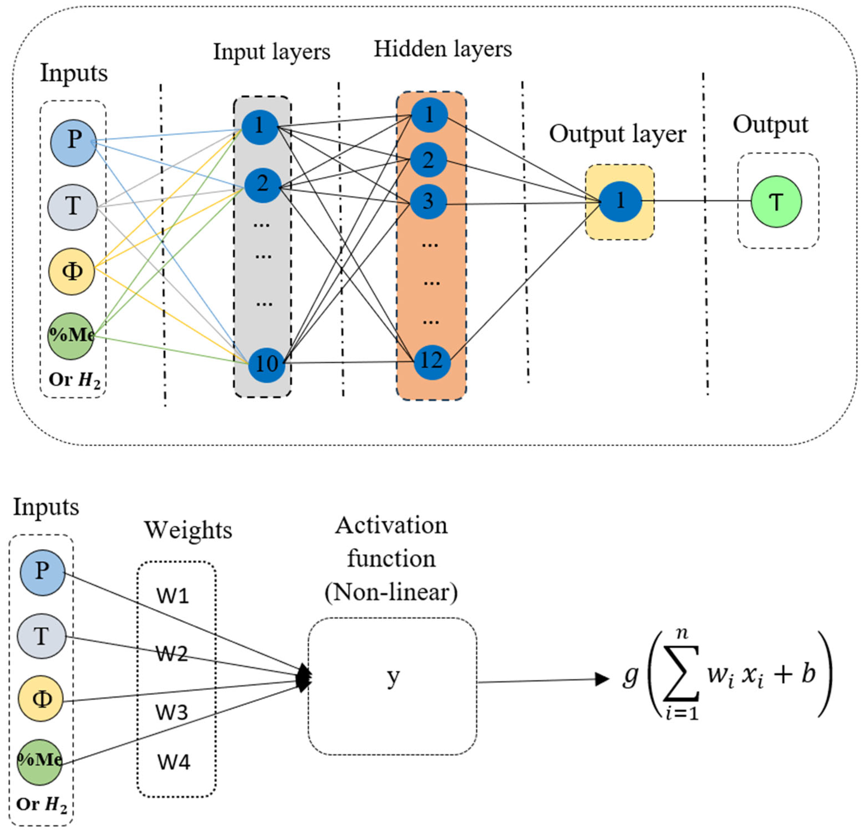
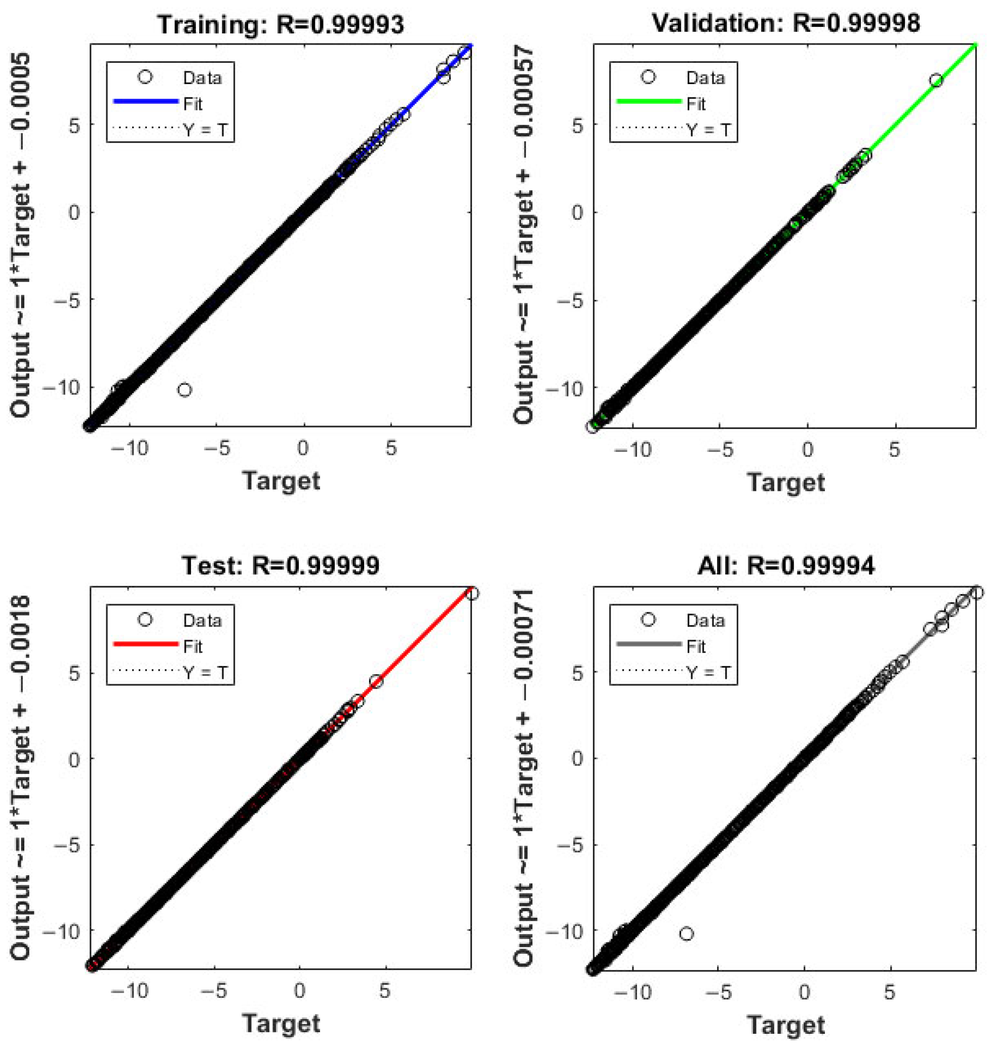
3.2.1. Artificial Neural Network (ANN)

Artificial Neural Networks (ANNs) are computational models that work similarly to the human brain. ANNs are used in a wide range of topics for classification, regression, pattern recognition, and more [43]. Figure 3 depicts the general structure of the ANN employed in the present work. The inputs to the ANN are pressure (P), temperature (T), overall equivalence ratio (φ), and the molar percentage of methanol or hydrogen in the mixture, and the output is the ignition delay. The ANN consists of neurons organized in layers: an input layer including ten neurons, one hidden layer including 12 neurons, and an output layer. The neurons of a layer are individually linked to each neuron of the next layer via a connection with a specific weight. When a neuron receives inputs from neurons of the prior layer, each input is multiplied by the related weight of the connection. The small random values are initially used for the weights. During training, these weights are revised using optimization algorithms to reach the minimum error in the network’s predictions. Each neuron also has a related bias term. After adding the weighted inputs, the bias is added to this sum. This process leads to non-zero output values even when all inputs are zero. After the weighted sum and bias addition, the result is passed through a transfer function (like sigmoid, hyperbolic tangent sigmoid, or Rectified Linear Unit), which makes the network non-linear. The network requires this non-linearity to deal with complex data. Overall, the primary function of ANNs is to minimize the error between predicted and target values by modifying the constants within the transfer functions between layers. Thus, selecting the transfer function and the specific errors in the training process are very important.

In the present study, the Levenberg–Marquardt algorithm is employed as the training function, while the mean squared error (MSE) method is used to evaluate the network’s performance. Data division is random. Random data division in ANNs refers to randomly splitting the dataset into different groups for training, validation, and testing. Consequently, diverse and representative data are used in the model’s performance evaluation. It will decrease the possibility of overfitting and provide a more precise assessment of its generalization capability.

The data are divided into three randomly discretized sets, for training, test, and validation. Approximately 70% of the data are used to train the network, 15% for testing, and the final 15% for validation. Figure 4 and Figure 5 present diagrams comparing the model output (y-axis) with the target values (x-axis) for these three datasets, as well as for the complete data set. In the diagrams, the more data points (shown as circles) lie on the “Fit” line, the better the model’s performance. According to the figures, the results demonstrate that the prediction accuracy (R) for training, validation, and testing exceeds 99% for both methanol/diesel and hydrogen/diesel ignition delay time data, indicating excellent model performance. The mean square errors for the best performance are 0.00066 and 0.000042 for methanol/diesel and hydrogen/diesel, respectively.

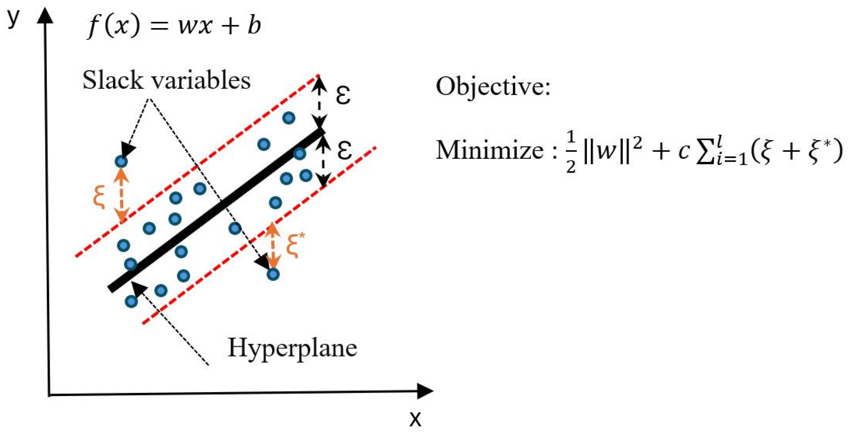
3.2.2. Support Vector Regression (SVR)

Support Vector Regression (SVR) is a machine learning algorithm based on so-called Support Vector Machines (SVM). It is widely used for regression tasks where a continuous target variable needs to be predicted [43]. SVR involves the principles of SVM, which is traditionally used for classification and regression problems. Traditional regression methods minimize the error directly, whereas SVR employs an ε-insensitive loss function. This means errors within a certain distance (ε) from the actual values are ignored, as illustrated in Figure 6. The model is only affected by data points that fall outside the ε margin (ξ and ${\mathsf{\xi }}^{\mathrm{*}}$). These crucial points, named support vectors, determine the position and direction of the regression line. A regularization parameter (C) is responsible for managing the compromise between the flatness of the regression function and the amount to which a deviation larger than ε is allowed. A larger C value leads to a more correct model that may overfit, while a smaller C allows for a more generalized model. SVR employs different kernels to deal with non-linear trends. Common kernels include linear kernel, polynomial kernel, and Gaussian kernel. This study trains the model using the Gaussian and polynomial kernels because the data show nonlinear trends.

Figure 7 and Figure 8 show diagrams comparing the SVR-predicted values (y-axis) with the observed values (x-axis) using two different kernel functions: (a) Gaussian and (b) Polynomial. These diagrams illustrate how closely the predicted values match the observed data. The more blue points that lie on the red line (“Fit”), the more accurate the trained model is. Both kernels demonstrate good performance for both methanol/diesel and hydrogen/diesel. According to the results, error values for hydrogen/diesel models are 0.9895 for the Gaussian method and 0.9802 for the polynomial method. For methanol/diesel models, the error values are 0.9947 and 0.9939, respectively.

Both machine learning methods demonstrate high accuracy in predicting the targets. However, because the training time for the ANN method is approximately five times shorter, this method is selected for the remainder of this this work.

It is worth mentioning that statistical processing can enhance the reliability of simulation-based studies by evaluating the impact of input parameters. Techniques like the Taguchi design improve efficiency by reducing the number of simulations needed. Similar methods have been successfully applied in engineering, such as in Milojević et al. [44], to optimize system performance.

Before explaining how the ANN method is integrated into the engine simulation software, the software used in this work is first introduced.

3.3. Multi-Zone Dual-Fuel Combustion Model in GT-Power

This study employs GT-SUITE’s predictive dual-fuel multi-zone combustion model to simulate a medium-speed dual-fuel engine. Researchers have previously used this model to simulate dual-fuel combustion of methane and diesel [45,46]. Three primary models are integrated into a multi-zone model to simulate dual-fuel combustion, to try to capture the physics of an autoigniting pilot spray that burns in a non-premixed mode and in turn ignites a premixed fuel-air mixture that burns in a flame propagation mode: a spray model (EngCylCombDIPulse), a transition function from spray to flame, and the flame model (SITurb). Different sub-models are employed by the DIPulse model to estimate spray entrainment, ignition delay, premixed combustion, and diffusion combustion, all referring to the pilot injection. The primary strategy involves tracking the fuel from injection, through evaporation, and mixing with the gas around the diesel spray, until it burns. The cylinder mixture is divided into three thermodynamic zones, each of which has its own species and temperature. The outer zone is called the main unburned zone, containing all cylinder content at intake valve closing time (IVC). The spray unburned zone is the inner zone, which includes injected fuel and entrained gas. There is a third zone between the mentioned zones called the burned zone, holding combustion products [46].

The Arrhenius equation presented in Equation (2) is used to estimate the ignition delay time of the blend in the pilot injection. The Ignition Delay Multiplier ($C_{ign}$) can be used to adjust the equation.

$${\mathsf{\tau }}_{\mathrm{i}\mathrm{g}\mathrm{n}}={\mathrm{C}}_{\mathrm{i}\mathrm{g}\mathrm{n}}{\mathsf{\rho }}^{-1.5}\mathrm{e}\mathrm{x}\mathrm{p}({\displaystyle \frac{3500}{\mathrm{T}}}){\left[{\mathrm{O}}_2\right]}^{-0.5}$$

(2)

The Livengood–Wu integral [47] is a commonly used method in ignition delay modeling. It relies on the conservation of delay principle, which states that the total ignition delay can be calculated by adding up the instantaneous ignition delays starting from the injection. Ignition, and thus the start of combustion, happens when the time integral equals one as is indicated in Equation (3).

$${\int }_{{\mathrm{t}}_{\mathrm{S}\mathrm{O}\mathrm{I}}}^{{\mathrm{t}}_{\mathrm{S}\mathrm{O}\mathrm{C}}}{\displaystyle \frac{1}{{\mathsf{\tau }}_{\mathrm{i}\mathrm{g}\mathrm{n}}\left(\mathrm{t}\right)}}=1$$

(3)

Dierickx et al. [36] compared the GT-Power correlation and several other correlations for predicting the ignition delay of methanol–diesel and hydrogen–diesel co-combustion, using measured data from a medium-speed marine engine under real-world conditions. They found that the GT-Power methodology accurately predicts ignition delay in diesel-only applications but fails to do so when the methanol energy fraction increases.

The next section explains how the ANN was incorporated into this modeling framework.

3.4. Integration of the ANN into the Multi-Zone Dual-Fuel Combustion Model in GT-Power

To integrate the ANN from Section 3.2.1. into the dual-fuel multi-zone combustion model in GT-Power, it is first converted into a mathematical formula using its weights ($w$), biases ($b$), and transfer functions ($f$) [42].

The equation that relates the input and output parameters can be obtained as follows:

$$\mathrm{z}={\mathrm{f}}_{\mathrm{o}\mathrm{u}\mathrm{t}}\left\{\left(\begin{array}{ccc}{\mathrm{w}}_{11}& {\mathrm{w}}_{12}\dots & {\mathrm{w}}_{1\mathrm{h}}\end{array}\right)\times {\mathrm{f}}_{\mathrm{h}\mathrm{i}\mathrm{d}\mathrm{d}\mathrm{e}\mathrm{n}}\left\{\left(\begin{array}{ccc}{\mathrm{w}}_{11}& \dots & {\mathrm{w}}_{1\mathrm{i}}\\ ⋮& \ddots & ⋮\\ {\mathrm{w}}_{\mathrm{h}1}& \dots & {\mathrm{w}}_{\mathrm{h}\mathrm{i}}\end{array}\right)\times {\mathrm{f}}_{\mathrm{i}\mathrm{n}\mathrm{p}\mathrm{u}\mathrm{t}}\left\{\left(\begin{array}{ccc}{\mathrm{w}}_{11}& \dots & {\mathrm{w}}_{14}\\ ⋮& \ddots & ⋮\\ {\mathrm{w}}_{\mathrm{i}1}& \dots & {\mathrm{w}}_{\mathrm{i}4}\end{array}\right)\times \left(\begin{array}{c}{\mathrm{y}}_1\\ {\mathrm{y}}_2\\ {\mathrm{y}}_3\\ {\mathrm{y}}_4\end{array}\right)+{\mathrm{b}}_{\mathrm{i}}\right\}+{\mathrm{b}}_{\mathrm{h}}\right\}+{\mathrm{b}}_{\mathrm{O}}\right\}$$

(4)

where ${\mathrm{f}}_{\mathrm{o}\mathrm{u}\mathrm{t}}$, ${\mathrm{f}}_{\mathrm{h}\mathrm{i}\mathrm{d}\mathrm{d}\mathrm{e}\mathrm{n}}$, ${\mathrm{f}}_{\mathrm{i}\mathrm{n}\mathrm{p}\mathrm{u}\mathrm{t}}$ are the transfer functions of the output layer, hidden layer, and input layer, respectively, and ${\mathrm{b}}_{\mathrm{o}}$, ${\mathrm{b}}_{\mathrm{h}}$, ${\mathrm{b}}_{\mathrm{i}}$ are the biases of the output layer, hidden layer and input layer. The scaled output (z) should be de-normalized using Equation (1) to obtain the actual output. This involves using the maximum and minimum values of the target data during the descaling process.

GT-Power software facilitates the development of new models for parameters such as ignition delay and flame speed through user-defined codes. The DIPulse user code, explained in the previous section, can be employed to incorporate user-defined models for estimating ignition delay time. It provides access to pulse conditions such as pulse temperature, cylinder pressure, and pulse composition.

In this study, the user code is used to implement a trained neural network for calculating ${\mathsf{\tau }}_{\mathrm{i}\mathrm{g}\mathrm{n}}$ in Equation (3), using the pulse conditions (P, T, φ, and methanol or hydrogen molar percentage) as inputs.

3.5. Look-Up Table and Correlation Methods

Another approach to incorporate the ignition delay data from Section 3.1. into the multi-zone combustion model is through the use of a look-up table. Initially, a look-up table is generated to cover a wide range of operating conditions that covers all scenarios occurring during the injection pulse. Subsequently, specific commands are implemented in the DIPulse user code to retrieve ${\mathsf{\tau }}_{\mathrm{i}\mathrm{g}\mathrm{n}}$(t) as per Equation (3) from the look-up table.

As a final alternative, the phenomenological correlation proposed by Dierickx et al. [36] is also employed in this work to estimate the ignition delay. They developed a new correlation for dual-fuel operation with hydrogen or methanol in a medium speed single cylinder engine. Their approach emphasizes the importance of incorporating additional terms, such as the methanol equivalence ratio, to accurately describe methanol’s inhibition effect. More detailed information about their correlation can be obtained from their paper [36].

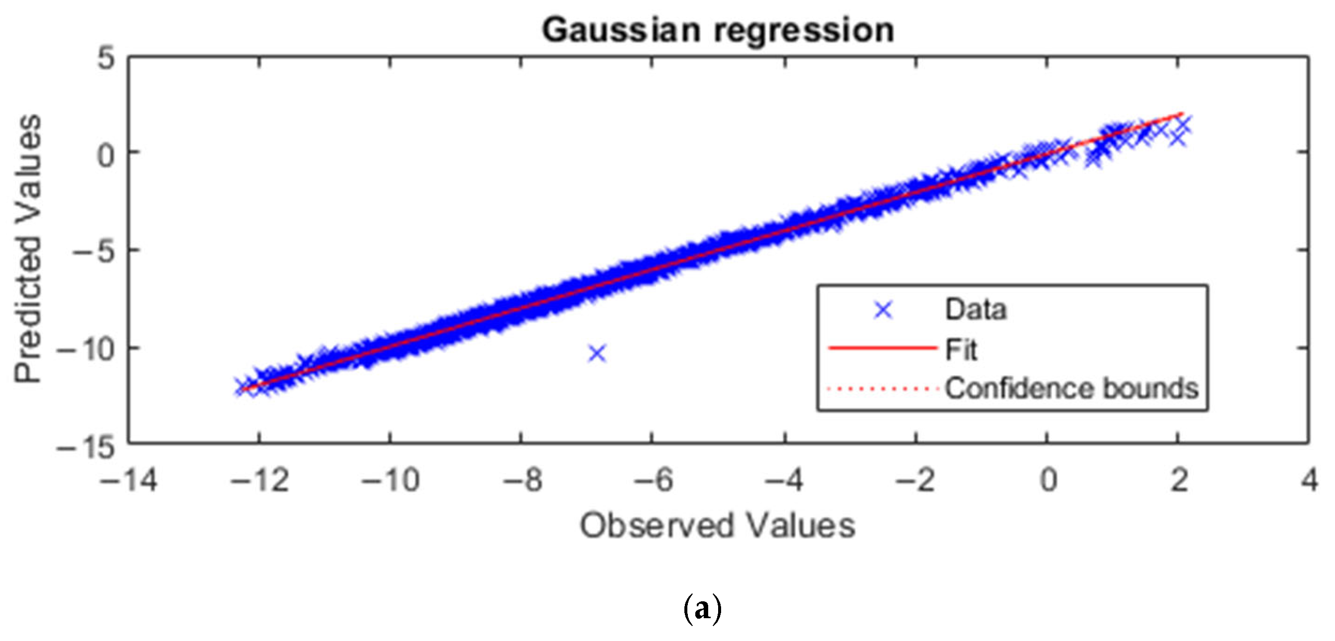
4. Results and Discussions

The mentioned methods are now used to predict the ignition delay after being integrated in a multi-zone combustion model and the results are compared to the experimental data from the medium-speed dual-fuel engine as listed in Section 2. The final goal is to see which method most accurately predicts the ignition delay in real-world engine conditions.

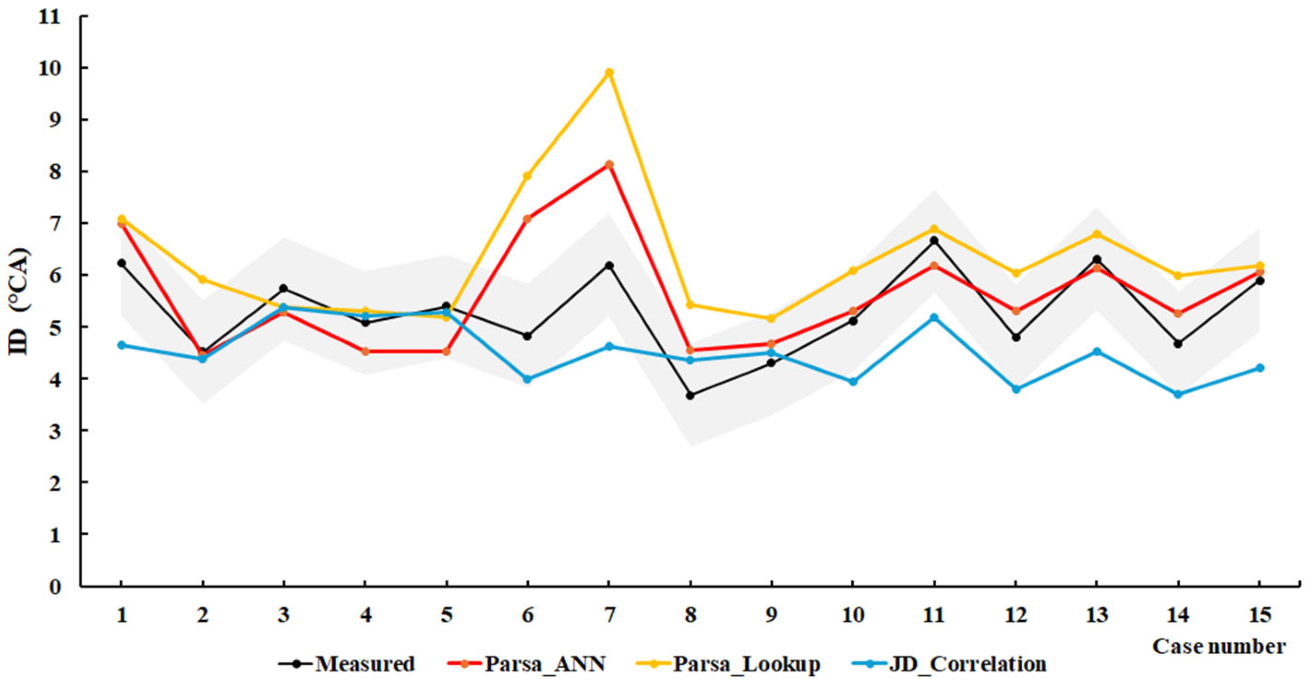
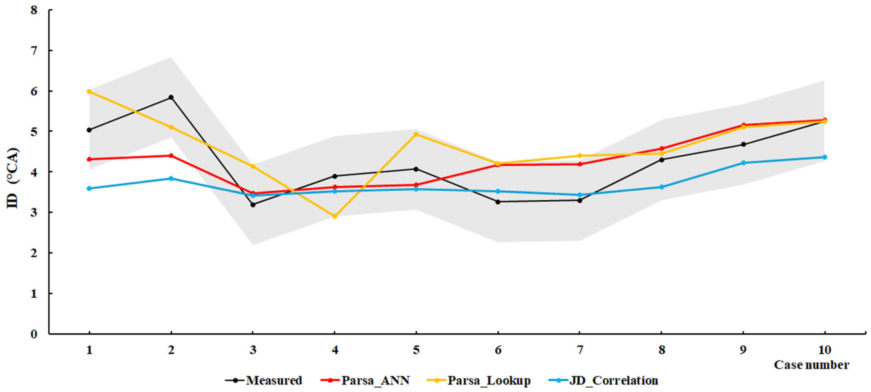
4.1. Methanol/Diesel

Figure 9 and Figure 10 compare the ignition delay predictions for the SCE1 and SCE2 methanol/diesel dual-fuel engine data points (as listed in Table 2) using the different methodologies. It should be mentioned that the measure ignition delay is derived from in-cylinder pressure data and is defined as the crank angle at which 2% of the total fuel mass has been burned. This point is commonly used as a reliable indicator of the start of combustion (SOC), as it captures the transition from fuel injection to the onset of significant heat release. To determine this, the apparent heat release rate is first calculated from the pressure trace using the first law of thermodynamics, and then integrated to obtain the cumulative heat release. The resulting mass fraction burned curve allows identification of the 2% burn point, which provides a consistent basis for comparing ignition delays under varying engine operating conditions. The gray area represents the measurement resolution of 1 crank angle degree. The methanol energy fraction varies from 50% to 75% for the SCE1 cases and from 46% to 56% for the SCE2 cases. It can be seen from both figures that the ignition delay of the pilot diesel is significantly influenced by increasing the methanol percentage in the premixed fuel under real engine conditions, which is in good agreement with the findings of previous works [32]. Ignition delay is represented in crank angle in the figures. It is worth mentioning that one crank angle degree at 1000 RPM is equal to 166.7 microseconds.

According to Figure 9, the results from the ANN show more accurate predictions of ignition delay compared to other methods. The average relative errors of the ANN, correlation, and lookup table methods are 13%, 17%, and 23%, respectively. Furthermore, the ANN method has the lowest RMSE, approximately 0.91, compared to around 1.09 and 1.52 for the correlation and lookup table methods, respectively. In addition, as shown in

Table 4. Comparison of RMSE and MSRE for the different methodologies.

Engine	Methodology	Root Mean Square Error (RMSE)	Mean Squared Relative Error (MSRE)
SCE1	Parsa_ANN	0.9127	0.0314
	Parsa_LookUP	1.5192	0.0894
	JD_Correlation	1.0909	0.0366
SCE2	Parsa_ANN	0.6939	0.1640
	Parsa_LookUP	0.7927	0.2115
	JD_Correlation	0.8996	0.1733

, the ANN method has a lower mean squared relative error (MSRE) of 0.03. The MSRE is 0.04 for the correlation method and 0.09 for the lookup table.

Figure 10 demonstrates the ignition delay predictions of the different methods for the SCE2 cases. It can be seen that here, too, that the ANN method predicts the ignition delay time more accurately compared to the other two methods. The average relative error of the ANN method is about 14%, which is lower than that of the correlation and lookup table methods, at 15% and 18.17%, respectively. Moreover, Table 4 shows that the ANN method has the lowest RMSE and MSRE, at approximately 0.7 and 0.2, respectively. Additionally, in terms of running time, the ANN and correlation methods are about 40% faster than using the lookup table.

The low accuracy of the lookup table method can be attributed to several factors: the four input data points required for prediction, the strongly non-linear trend of the ignition delay time, and the interpolation technique used. The interpolation method and the number of data points used to create the lookup table are critical factors affecting its accuracy in such situations. However, increasing the size of the lookup table and employing more complex interpolation methods will result in longer running times.

It can be concluded that the ANN methodology is the most accurate for predicting the ignition delay time of a methanol/diesel dual-fuel engine under real engine conditions. Since the data is derived from chemical kinetics mechanisms, developing a more accurate mechanism can potentially further enhance this method’s accuracy.

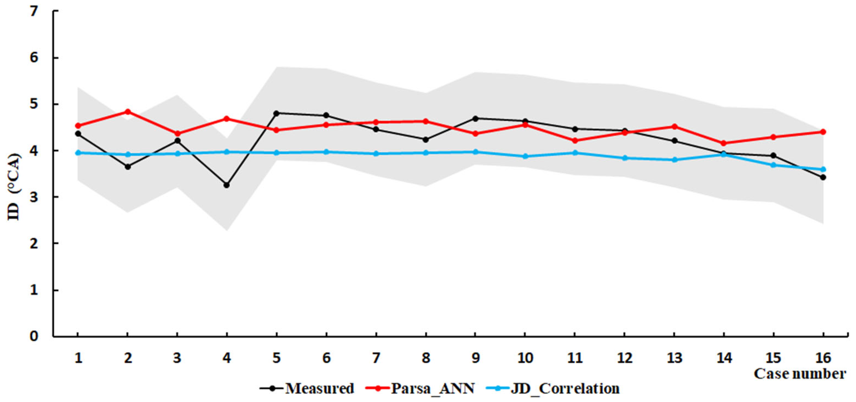
4.2. Hydrogen/Diesel

Figure 11 compares the ignition delay predictions for the hydrogen/diesel operation using two different methods, ANN and correlation, against the experimental data for SCE1. There are 12 cases, and the hydrogen energy fraction (HEF) changes between 25% and 50%. The results from both methods indicate that the ignition delay of the diesel pilot is not considerably affected by the percentage of hydrogen in the premixed fuel under real-world engine conditions. This finding aligns with results from other literature [32].

The average relative error of both methods is about 10.9%. Furthermore, the RMSE is 0.57 for the ANN method and 0.53 for the correlation method. Both methods show good accuracy in predicting the ignition delay time of the diesel pilot in the presence of a hydrogen/air mixture. The ANN and correlation methods both show the same running time.

5. Conclusions

Accurate estimation of the ignition delay time of the pilot fuel is essential for simulating methanol/diesel and hydrogen/diesel dual-fuel combustion. There has been insufficient investigation into calculating this ignition delay under real engine conditions. This study aimed to determine the most accurate method for estimating ignition delay times in methanol/diesel and hydrogen/diesel dual-fuel engines under real world conditions. Data were used from a medium speed single cylinder setup running in relevant conditions, to serve as validation data. Unlike traditional correlations that require calibration based on specific engine parameters to produce accurate results, the proposed methodologies in this work can principally be used to calculate ignition delay in any dual-fuel engine. For the SCE1 dataset, the ANN achieved an RMSE of 0.91, outperforming the correlation method (RMSE = 1.09) and the lookup table method (RMSE = 1.52). Similarly, for the SCE2 dataset, the ANN method achieved the lowest RMSE of 0.7. For hydrogen/diesel operation, both ANN and correlation methods achieved good accuracy, with average relative errors of ~10.9% and RMSE values of 0.57 and 0.53, respectively. Additionally, the ANN method is approximately 40% faster than the lookup table methodology in terms of running time.

References

1. Faber, J.; Hanayama, S.; Zhang, S.; Pereda, P.; Comer, B.; Hauerhof, E.; van der Loeff, W.S.; Smith, T.; Zhang, Y.; Kosaka, H. Reduction of GHG emissions from ships—Fourth IMO GHG study 2020—Final report. IMO MEPC 2020, 75, 15. [Google Scholar]
2. Dnv, G. Maritime Forecast to 2050, Energy Transition Outlook 2019; DNV GL: Høvik, Norway, 2019. [Google Scholar]
3. Fetting, C. The European Green Deal; ESDN Report; ESDN Office: Vienna, Austria, 2020; p. 2. [Google Scholar]
4. Hedberg, A. The European Green Deal: How to Turn Ambition into Action; EPC Discussion Paper 04 November 2021; EPC: Brussels, Belgium, 2021. [Google Scholar]
5. Verhelst, S.; Turner, J.W.; Sileghem, L.; Vancoillie, J. Methanol as a fuel for internal combustion engines. Prog. Energy Combust. Sci. 2019, 70, 43–88. [Google Scholar] [CrossRef]
6. Huang, Z. Fuel blend combustion for decarbonization. Proc. Combust. Inst. 2024, 40, 105776. [Google Scholar] [CrossRef]
7. Hosseini, S.H.; Tsolakis, A.; Alagumalai, A.; Mahian, O.; Lam, S.S.; Pan, J.; Peng, W.; Tabatabaei, M.; Aghbashlo, M. Use of hydrogen in dual-fuel diesel engines. Prog. Energy Combust. Sci. 2023, 98, 101100. [Google Scholar] [CrossRef]
8. Verhelst, S. Recent progress in the use of hydrogen as a fuel for internal combustion engines. Int. J. Hydrogen Energy 2014, 39, 1071–1085. [Google Scholar] [CrossRef]
9. Olah, G.A. After oil and gas: Methanol economy. Catal. Lett. 2004, 93, 1–2. [Google Scholar] [CrossRef]
10. Tian, Z.; Wang, Y.; Zhen, X.; Liu, Z. The effect of methanol production and application in internal combustion engines on emissions in the context of carbon neutrality: A review. Fuel 2022, 320, 123902. [Google Scholar] [CrossRef]
11. Gautam, P.; Upadhyay, S.N.; Dubey, S. Bio-methanol as a renewable fuel from waste biomass: Current trends and future perspective. Fuel 2020, 273, 117783. [Google Scholar] [CrossRef]
12. Lonis, F.; Tola, V.; Cau, G. Assessment of integrated energy systems for the production and use of renewable methanol by water electrolysis and CO2 hydrogenation. Fuel 2021, 285, 119160. [Google Scholar] [CrossRef]
13. Geo, V.E.; Nagarajan, G.; Nagalingam, B. Experimental investigations to improve the performance of rubber seed oil–fueled diesel engine by dual fueling with hydrogen. Int. J. Green Energy 2009, 6, 343–358. [Google Scholar] [CrossRef]
14. Parsa, S.; Jafarmadar, S.; Neshat, E. Application of waste heat in a novel trigeneration system integrated with an HCCI engine for power, heat and hydrogen production. Int. J. Hydrogen Energy 2022, 47, 26303–26315. [Google Scholar] [CrossRef]
15. Basile, A.; Dalena, F. Methanol: Science and Engineering; Elsevier: Amsterdam, The Netherlands, 2017. [Google Scholar]
16. Agarwal, A.K.; Valera, H.; Pexa, M.; Čedík, J. Methanol: A Sustainable Transport Fuel for CI Engines; Springer Nature: Berlin/Heidelberg, Germany, 2021. [Google Scholar] [CrossRef]
17. Jiang, M.; Sun, W.; Guo, L.; Zhang, H.; Jia, Z.; Qin, Z.; Zhu, G.; Yu, C.; Zhang, J. Numerical optimization of injector hole arrangement for marine methanol/diesel direct dual fuel stratification engines. Appl. Therm. Eng. 2024, 257, 124456. [Google Scholar] [CrossRef]
18. Li, Z.; Wang, Y.; Yin, Z.; Geng, H.; Zhu, R.; Zhen, X. Effect of injection strategy on a diesel/methanol dual-fuel direct-injection engine. Appl. Therm. Eng. 2021, 189, 116691. [Google Scholar] [CrossRef]
19. Dierickx, J.; Verbiest, J.; Janvier, T.; Peeters, J.; Sileghem, L.; Verhelst, S. Retrofitting a high-speed marine engine to dual-fuel methanol-diesel operation: A comparison of multiple and single point methanol port injection. Fuel Commun. 2021, 7, 100010. [Google Scholar] [CrossRef]
20. Yao, C.; Pan, W.; Yao, A. Methanol fumigation in compression-ignition engines: A critical review of recent academic and technological developments. Fuel 2017, 209, 713–732. [Google Scholar] [CrossRef]
21. Saravanan, N.; Nagarajan, G. Performance and emission studies on port injection of hydrogen with varied flow rates with Diesel as an ignition source. Appl. Energy 2010, 87, 2218–2229. [Google Scholar] [CrossRef]
22. Fayaz, H.; Saidur, R.; Razali, N.; Anuar, F.S.; Saleman, A.; Islam, M. An overview of hydrogen as a vehicle fuel. Renew. Sustain. Energy Rev. 2012, 16, 5511–5528. [Google Scholar] [CrossRef]
23. Havemann, H.; Rao, M.; Natarajan, A.; Narasimhan, T. Alcohol in diesel engines. J. Indian Inst. Sci. 2008, 88, 820. [Google Scholar]
24. Zhang, Z.; Tsang, K.; Cheung, C.S.; Chan, T.L.; Yao, C. Effect of fumigation methanol and ethanol on the gaseous and particulate emissions of a direct-injection diesel engine. Atmos. Environ. 2011, 45, 2001–2008. [Google Scholar] [CrossRef]
25. Shi, M.; Wu, B.; Wang, J.; Jin, S.; Chen, T. Optimization of methanol/diesel dual-fuel engines at low load condition for heavy-duty vehicles to operated at high substitution ratio by using single-hole injector for direct injection of methanol. Appl. Therm. Eng. 2024, 246, 122854. [Google Scholar] [CrossRef]
26. Imran, A.; Varman, M.; Masjuki, H.H.; Kalam, M.A. Review on alcohol fumigation on diesel engine: A viable alternative dual fuel technology for satisfactory engine performance and reduction of environment concerning emission. Renew. Sustain. Energy Rev. 2013, 26, 739–751. [Google Scholar] [CrossRef]
27. Sun, Z.; Lian, Z.; Ma, J.; Wang, C.; Li, W.; Pan, J. Combustion and Emissions Optimization of Diesel–Methanol Dual-Fuel Engine: Emphasis on Valve Phasing and Injection Parameters. Processes 2025, 13, 1183. [Google Scholar] [CrossRef]
28. Verhelst, S.; Wallner, T. Hydrogen-fueled internal combustion engines. Prog. Energy Combust. Sci. 2009, 35, 490–527. [Google Scholar] [CrossRef]
29. Liew, C.; Li, H.; Nuszkowski, J.; Liu, S.; Gatts, T.; Atkinson, R.; Clark, N. An experimental investigation of the combustion process of a heavy-duty diesel engine enriched with H2. Int. J. Hydrogen Energy 2010, 35, 11357–11365. [Google Scholar] [CrossRef]
30. Chintala, V.; Subramanian, K. A comprehensive review on utilization of hydrogen in a compression ignition engine under dual fuel mode. Renew. Sustain. Energy Rev. 2017, 70, 472–491. [Google Scholar] [CrossRef]
31. Karagöz, Y.; Sandalcı, T.; Yüksek, L.; Dalkılıç, A.S.; Wongwises, S. Effect of hydrogen–diesel dual-fuel usage on performance, emissions and diesel combustion in diesel engines. Adv. Mech. Eng. 2016, 8, 1687814016664458. [Google Scholar] [CrossRef]
32. Parsa, S.; Verhelst, S. Numerical Investigation of the Ignition Delay and Laminar Flame Speed for Pilot-Ignited Dual Fuel Engine Operation with Hydrogen or Methanol; 0148-7191; SAE Technical Paper; SAE: Warrendale, PA, USA, 2023. [Google Scholar]
33. Coulier, J.; Verhelst, S. Using alcohol fuels in dual fuel operation of compression ignition engines: A review. In Proceedings of the 28th CIMAC World Congress on Combustion Engine, Helsinki, Finland, 6–10 June 2016; pp. 1–12. [Google Scholar]
34. Yin, Z.; Yao, C.; Geng, P.; Hu, J. Visualization of combustion characteristic of diesel in premixed methanol–air mixture atmosphere of different ambient temperature in a constant volume chamber. Fuel 2016, 174, 242–250. [Google Scholar] [CrossRef]
35. Dhole, A.; Yarasu, R.; Lata, D. Investigations on the combustion duration and ignition delay period of a dual fuel diesel engine with hydrogen and producer gas as secondary fuels. Appl. Therm. Eng. 2016, 107, 524–532. [Google Scholar] [CrossRef]
36. Dierickx, J.; Mattheeuws, L.; Christianen, K.; Stenzel, K.; Verhelst, S. Evaluation and extension of ignition delay correlations for dual-fuel operation with hydrogen or methanol in a medium speed single cylinder engine. Fuel 2023, 345, 128254. [Google Scholar] [CrossRef]
37. Zang, R.; Yao, C. Numerical study of combustion and emission characteristics of a diesel/methanol dual fuel (DMDF) engine. Energy Fuels 2015, 29, 3963–3971. [Google Scholar] [CrossRef]
38. Xu, H.; Yao, C.; Xu, G. Chemical kinetic mechanism and a skeletal model for oxidation of n-heptane/methanol fuel blends. Fuel 2012, 93, 625–631. [Google Scholar] [CrossRef]
39. Decan, G.; Lucchini, T.; D’Errico, G.; Verhelst, S. A novel technique for detailed and time-efficient combustion modeling of fumigated dual-fuel internal combustion engines. Appl. Therm. Eng. 2020, 174, 115224. [Google Scholar] [CrossRef]
40. Andrae, J.C.; Head, R. HCCI experiments with gasoline surrogate fuels modeled by a semidetailed chemical kinetic model. Combust. Flame 2009, 156, 842–851. [Google Scholar] [CrossRef]
41. Liu, S.; Sun, T.; Zhou, L.; Jia, M.; Zhao, W.; Wei, H. A new skeletal kinetic model for methanol/n-heptane dual fuels under engine-like conditions. Energy 2023, 263, 125648. [Google Scholar] [CrossRef]
42. Lawal, A.I. An artificial neural network-based mathematical model for the prediction of blast-induced ground vibration in granite quarries in Ibadan, Oyo State, Nigeria. Sci. Afr. 2020, 8, e00413. [Google Scholar] [CrossRef]
43. Shahpouri, S.; Norouzi, A.; Hayduk, C.; Fandakov, A.; Rezaei, R.; Koch, C.R.; Shahbakhti, M. Laminar flame speed modeling for low carbon fuels using methods of machine learning. Fuel 2023, 333, 126187. [Google Scholar] [CrossRef]
44. Milojević, S.; Savić, S.; Mitrović, S.; Marić, D.; Krstić, B.; Stojanović, B.; Popović, V. Solving the problem of friction and wear in auxiliary devices of internal combustion engines on the example of reciprocating air compressor for vehicles. Teh. Vjesn. 2023, 30, 122–130. [Google Scholar]
45. Wenig, M.; Roggendorf, K.; Fogla, N. Towards predictive dual-fuel combustion and prechamber modeling for large two-stroke engines in the scope of 0D/1D simulation. In Proceedings of the 29th CIMAC World Congress on Combustion Engine Technology, Vancouver, BC, Canada, 10–14 June 2019; pp. 10–14. [Google Scholar]
46. Millo, F.; Accurso, F.; Piano, A.; Caputo, G.; Cafari, A.; Hyvönen, J. Experimental and numerical investigation of the ignition process in a large bore dual fuel engine. Fuel 2021, 290, 120073. [Google Scholar] [CrossRef]
47. Livengood, J.; PC, W. Correlation of autoignition phenomena in internal combustion engines and rapid compression machines. Symp. (Int.) Combust. 1955, 5, 347–356. [Google Scholar] [CrossRef]
Figure 1. In-cylinder pressure for different methanol energy fractions (MEF) at 1500 rpm and BMEP of 1.23 MPa. Adapted from [19]. As MEF rises, the start of combustion, shown by the pressure rise rate increase (marked with a red circle), moves to a later point in the engine cycle.
Energies 18 03064 g001
Figure 2. Picture of experimental setup. Methanol fuel supply system: 1: magnetic valve, 2: flexible hose pipe, 3: pressure sensor, 4: methanol injector, 5: surge tank [36].
Energies 18 03064 g002
Figure 3. Artificial neural network architecture (w, x, b and g are weights, inputs, bias and activation function, respectively).
Energies 18 03064 g003
Figure 4. Regression results of the training for the methanol/diesel data set.
Energies 18 03064 g004
Figure 5. Regression results of ANN training for the hydrogen/diesel data set.
Energies 18 03064 g005
Figure 6. Linear SVR (w, b, c, Ɛ and ξ are weight, bias, regularization parameter, margin and slack variables, respectively). The red dotted lines indicate the boundaries of the ε-insensitive tube, within which no penalty is given for errors.
Energies 18 03064 g006
Figure 7. Regression results of SVR training for methanol/diesel dataset using two different kernels: (a) Gaussian, (b) polynomial.
Energies 18 03064 g007aEnergies 18 03064 g007b
Figure 8. Regression results of SVR training for hydrogen/diesel dataset using two different kernels: (a) Gaussian, (b) polynomial.
Energies 18 03064 g008
Figure 9. Comparison of results from different methodologies with measured data (SCE1). The gray area represents the measurement resolution of 1 crank angle degree.
Energies 18 03064 g009
Figure 10. Comparison of results from different methodologies with measured data (SCE2). The gray area represents the measurement resolution of 1 crank angle degree.
Energies 18 03064 g010
Figure 11. Comparison of results from ANN and correlation methods with measured data (SCE1). The gray area represents the measurement resolution of 1 crank angle degree.
Energies 18 03064 g011