Impact of Models of Thermodynamic Properties and Liquid–Gas Mass Transfer on CFD Simulation of Liquid Hydrogen Release

Abstract

The safety performance of liquid hydrogen storage has a significant influence on its large-scale commercial application. Due to the complexity and costs of experimental investigation, computational fluid dynamics (CFD) simulations have been extensively applied to investigate the dynamic behaviors of liquid hydrogen release. The involved physical and chemical models, such as models of species thermodynamic properties and liquid–gas mass transfer, play a major role for the entire CFD model performance. However, comprehensive investigations into their impacts remain insufficient. In this study, CFD models of liquid hydrogen release were developed by using two widely used commercial simulation tools, Fluent and FLACS, and validated against experimental data available in the literature. Comparisons of the model results reveal strong discrepancies in the prediction accuracy of temperature and hydrogen volume fraction between the two models. The impact of the models of thermodynamic properties and liquid–gas mass transfer on the prediction results was subsequently explored by incorporating the FLACS sub-models to Fluent and evaluating the resulting prediction differences in temperatures and hydrogen volume fractions. The results show that the models of thermodynamic properties and liquid–gas mass transfer used in FLACS underestimate the vertical rise height and the highest hydrogen volume fraction of the cloud. Sensitivity analyses on the parameters in these sub-models indicate that the specific heats of hydrogen and nitrogen, in conjunction with the mass flow rate and outflow density of the mass transfer model, have a significant influence on model prediction of temperature.

1. Introduction

Hydrogen plays a vital role in advancing the low-carbon transformation of the transportation sector [1]. Liquid hydrogen presents significant potential for applications in aerospace, chemical, and transportation industries [2]. Compared to gaseous hydrogen, it provides advantages in energy density, purity, and economic viability for long-distance transportation [3]. However, its safety performance is a crucial prerequisite for large-scale commercial application, as its accidental leakage can lead to extreme consequences [4]. As the saturation temperature of liquid hydrogen is 20.3 K at atmospheric pressure, it must be stored under pressurized and cryogenic conditions [5]. When released, liquid hydrogen evaporates immediately because of the great differences between storage and atmospheric conditions [6]. The evaporated hydrogen mixes subsequently with air and forms a flammable gas cloud, which can be easily ignited and further explode by a spark source [7,8]. Given the significant consequences induced by liquid hydrogen leak, it is important to characterize and understand the dynamic behavior of liquid hydrogen release and explosion in order to ensure the safety use of liquid hydrogen [9,10,11].

In the past, experiments were conducted to explore the characteristics of liquid hydrogen release. Large-scale experiments were carried out by NASA (National Aeronautics and Space Administration, Washington, DC, USA) in 1981 [12]. Measurements on liquid hydrogen release between buildings were performed by BAM (Federal Institute for Materials Research and Testing, Berlin, Germany) [13], and tests on liquid hydrogen release in unobstructed scenarios were conducted by HSL (Health and Safety Laboratory, Derbyshire, UK) [14].

Compared to experimental approach, numerical simulations with CFD tools, such as Fluent [15] and FLACS [16], present advantages of lower costs and reduced risks [17] and thus were extensively applied to study the dynamic process of liquid hydrogen release. These tools incorporate physical and chemical models, such as those for combustion [18,19] as well as for mixing and diffusion [20,21], enabling a multi-physical description of the behaviors of liquid hydrogen release. To capture the dynamics of hydrogen release, the mixture model [19,20,21,22,23] and the pseudo source model [24,25,26] were often applied for the modeling of the two-phase flow of liquid and gaseous hydrogen. And the realizable $k-ϵ$ model [18,19,20,21] and the standard $k-ϵ$ model [24,25,26,27] were employed for turbulence modeling. The details of these models are introduced in the Mathematical Models Section. Schmidt et al. [27] developed a CFD model for the prediction of the safety distance for liquid hydrogen leakage between buildings with Fluent and validated the model against data reported by BAM. Sklavounos et al. [22] simulated the large-scale release of liquid hydrogen by using Fluent and derived a correlation between temperature and hydrogen concentration to describe the release behavior of liquid hydrogen near the release point. Pu et al. [23] compared the release and dispersion behavior of liquid hydrogen and liquid natural gas with Fluent in terms of their hazardous regions formed after the release. Middha et al. [24] developed a pool model with FLACS to evaluate the spread and evaporation of liquid hydrogen and validated the model against data reported by NASA. Also, with FLACS, Shen et al. [25] calculated the downwind distance and height of flammable cloud in a liquid hydrogen refueling station, and Hansen et al. [26] simulated liquid hydrogen leakage and its consequence caused by flame flashback in an enclosed container.

Studies were carried out to investigate the impact of important condition parameters on the prediction of the characteristics of liquid hydrogen release [19,23,28,29,30,31,32,33,34]. Regarding the parameters of hydrogen release, the effect of mass flow rate [23], gas phase mass fraction [28], release height, direction, and velocity [29] on the development of hydrogen flow was examined. For environmental factors, the influence of air condensation [30], ground thermal conductivity [31], and wind fields [32,33] on the flow field was investigated. In addition, the impact of parameters of application scenarios, such as dike around source [19] and garages and tunnels [34], on the behavior of liquid hydrogen release was explored. However, limited studies examined the effects of involved physical and chemical models, such as those of thermodynamic properties and liquid–gas mass transfer, on the prediction of liquid hydrogen release behavior, despite the fact that the differences in these sub-models can lead to significant discrepancies in model performance [28,35,36]. vom Lehn et al. [36] demonstrated that the values of specific heats of species affect the prediction accuracy of combustion targets by influencing the chemical equilibrium. Ichard et al. [28] revealed that the predicted shape of liquid hydrogen jet is sensitive to the mass fraction of species in gas phase at release outlet. Chen et al. [35] highlighted that the heat and mass transfers between liquid and gas hydrogen have an impact on the radius of individual liquid hydrogen droplets and thereby on the flame structure as well. The commercial CFD tools Fluent [15] and FLACS [16] employ different models for the thermodynamic properties of species and liquid–gas mass transfer at hydrogen outlet, as detailed in the Mathematical Models Section. By analyzing the impact of these models on the entire model performance, it is expected to identify key parameters that significantly affect the predictive accuracy and to provide valuable insights for model optimization.

Thus, the present study aims to investigate the impact of models of thermodynamic parameters and liquid–gas mass transfer on the simulation of liquid hydrogen release and to identify the important parameters in these sub-models. For this purpose, CFD models are first developed using two widely used commercial tools, Fluent [15] and FLACS [16], respectively. These models are subsequently validated against the HSL experimental data in the literature and compared in terms of prediction accuracy for temperatures and hydrogen volume fractions. By incorporating the FLACS [16] sub-models into Fluent [15] and evaluating the resulting prediction differences, the impacts of models of thermodynamic properties and liquid–gas mass transfer are explored. Furthermore, sensitivity analyses are carried out to identify the key parameters in these models that affect the prediction accuracy of temperature significantly.

The presentation of this paper is organized as follows: First, the experiment of liquid hydrogen release, which is considered as validation target, is briefly introduced in Section 2. Next, the mathematical CFD models are described in Section 3. Then, model validation is performed and the results are presented in Section 4. The impact of the models of thermodynamic properties and liquid–gas mass transfer on model performance are explored and the results are also shown in Section 4, in conjunction with those of the sensitivity analyses. The paper closes with a section of the major conclusions.

2. Experiment Description

A series of liquid hydrogen release tests was performed by the Health and Safety Laboratory (HSL). In these tests, liquid hydrogen was stored in a tank at a pressure of 0.2 MPa and released through a 0.0266 m vacuum insulated hose into an open, unobstructed environment [14]. Temperature sensors were placed in downwind directions of 1.5 m, 3 m, 4.5 m, 6 m, and 7.5 m and at heights of 0.25 m, 0.75 m, and 1.25 m. The horizontal test, whose release position is located at a height of 0.86 m above the ground and which is designated as Test 7, is considered in this study due to its extensive available data [28,30,37,38]. The detailed experimental conditions of Test 7 are summarized in

Table 1. Experimental conditions of HSL Test 7.

Parameter		Value
Release conditions	Diameter (m)	0.0266
	Height (m)	0.86
	Mass rate (kg/s)	0.071
	Direction	Horizontal
Weather conditions	Wind speed at 2.5 m (m/s)	2.9
	Ambient temperature (K)	284.5
	Relative humidity (%)	64

.

3. Modeling Approaches

3.1. Mathematical Models

The release of liquid hydrogen is modeled by solving three-dimensional, transient conservation equations of mass, momentum, and energy with the two widely used commercial CFD tools, Fluent [15] and FLACS [16].

The mass conservation equation is

$${\displaystyle \frac{\partial \rho }{\partial t}}+{\displaystyle \frac{\partial }{\partial x_j}}\left(\rho u_j\right)=0,$$

(1)

where $\rho$ is the density, $t$ is the time, $x$ is the spatial coordinate, and $u$ is the velocity component. Subscript $j$, ranging from 1 to 3, corresponds to the three orthogonal spatial dimensions.

The momentum conservation equation is

$${\displaystyle \frac{\partial }{\partial t}}\left(\rho u_i\right)+{\displaystyle \frac{\partial }{\partial x_j}}\left(\rho u_i{u}_j\right)=-{\displaystyle \frac{\partial p}{\partial x_i}}+{\displaystyle \frac{\partial }{\partial x_j}}\left(\left(\mu +{\mu }_t\right)\left({\displaystyle \frac{\partial u_j}{\partial x_i}}+{\displaystyle \frac{\partial u_i}{\partial x_j}}\right)\right)+\rho g_i,$$

(2)

where $p$ is the pressure, $\mu$ is the dynamic viscosity, ${\mu }_t$ is the turbulent viscosity, and $g_i$ is the gravitational acceleration component in direction $i$. Subscript $i$ denotes another spatial dimension, which is different from that represented by subscript $j$.

The energy conservation equation is

$${\displaystyle \frac{\partial }{\partial t}}\left(\rho h\right)+{\displaystyle \frac{\partial }{\partial x_j}}\left(\rho u_{j}h\right)={\displaystyle \frac{\partial }{\partial x_j}}\left({\displaystyle \frac{{\mu }_t}{{\sigma }_H}}{\displaystyle \frac{\partial h}{\partial x_j}}\right)+{\displaystyle \frac{dp}{dt}}+{\displaystyle \frac{\partial }{\partial x_j}}\left(\lambda {\displaystyle \frac{\partial T}{\partial x_j}}\right),$$

(3)

where $h$ is the specific enthalpy, $\lambda$ is the thermal conductivity, $T$ is the temperature, and ${\sigma }_H$ is the turbulent Prandtl number of enthalpy.

In this study, turbulence is simulated with the standard $k-ϵ$ model, which has been widely applied in simulating liquid hydrogen release. Application and validation examples can be found in the literature [28,30,39]. The transport equations for turbulent kinetic energy $k$ and the dissipation rate of turbulent kinetic energy $ϵ$ are given by

$${\displaystyle \frac{\partial }{\partial t}}\left(\rho k\right)+{\displaystyle \frac{\partial }{\partial x_i}}\left(\rho k{u}_i\right)={\displaystyle \frac{\partial }{\partial x_j}}\left[\left(\mu +{\displaystyle \frac{{\mu }_t}{{\sigma }_k}}\right){\displaystyle \frac{\partial k}{\partial x_j}}\right]+G_k+G_b-\rho ϵ-Y_M+S_k,$$

(4)

and

$${\displaystyle \frac{\partial }{\partial t}}\left(\rho ϵ\right)+{\displaystyle \frac{\partial }{\partial x_i}}\left(\rho ϵu_i\right)={\displaystyle \frac{\partial }{\partial x_j}}\left[\left(\mu +{\displaystyle \frac{{\mu }_t}{{\sigma }_{ϵ}}}\right){\displaystyle \frac{\partial ϵ}{\partial x_j}}\right]+C_{1ϵ}{\displaystyle \frac{ϵ}{k}}\left(G_k+{C_{3ϵ}G}_b\right)-C_{2ϵ}\rho {\displaystyle \frac{{ϵ}^2}{k}}+S_{ϵ},$$

(5)

respectively, where $G_k$ and $G_b$ represent the generation of turbulence kinetic energy due to the mean velocity gradients and due to buoyancy, respectively. $Y_M$ denotes the contribution of the fluctuating dilatation in compressible turbulence to the overall dissipation rate. $S_k$ and $S_{ϵ}$ are user-defined source terms, representing external contributions to the turbulent kinetic energy and its dissipation rate, respectively. In this study, they are both assumed to be zero. ${\sigma }_k$ and ${\sigma }_{ϵ}$ are the turbulent Prandtl numbers of $k$ and $ϵ$, respectively. $C_{1ϵ},C_{2ϵ},$ and $C_{3ϵ}$ are empirical constants. The values of turbulent Prandtl numbers and empirical constants used in the models are summarized in

Table 2. Values of turbulent Prandtl numbers and empirical constants.

${\mathit{\sigma }}_{\mathit{H}}$	${\mathit{\sigma }}_{\mathit{k}}$	${\mathit{\sigma }}_{\mathit{ϵ}}$	${\mathit{C}}_{1\mathit{ϵ}}$	${\mathit{C}}_{2\mathit{ϵ}}$	${\mathit{C}}_{3\mathit{ϵ}}$
0.7	1	1.3	1.44	1.92	0.8

.

The wall functions are applied to simulate the flow in the near-wall region following the recommendation of Fluent [15] and FLACS [16]. Details about the wall functions can be found in previous work by Visser et al. [40], Holborn et al. [31], and Shen et al. [25].

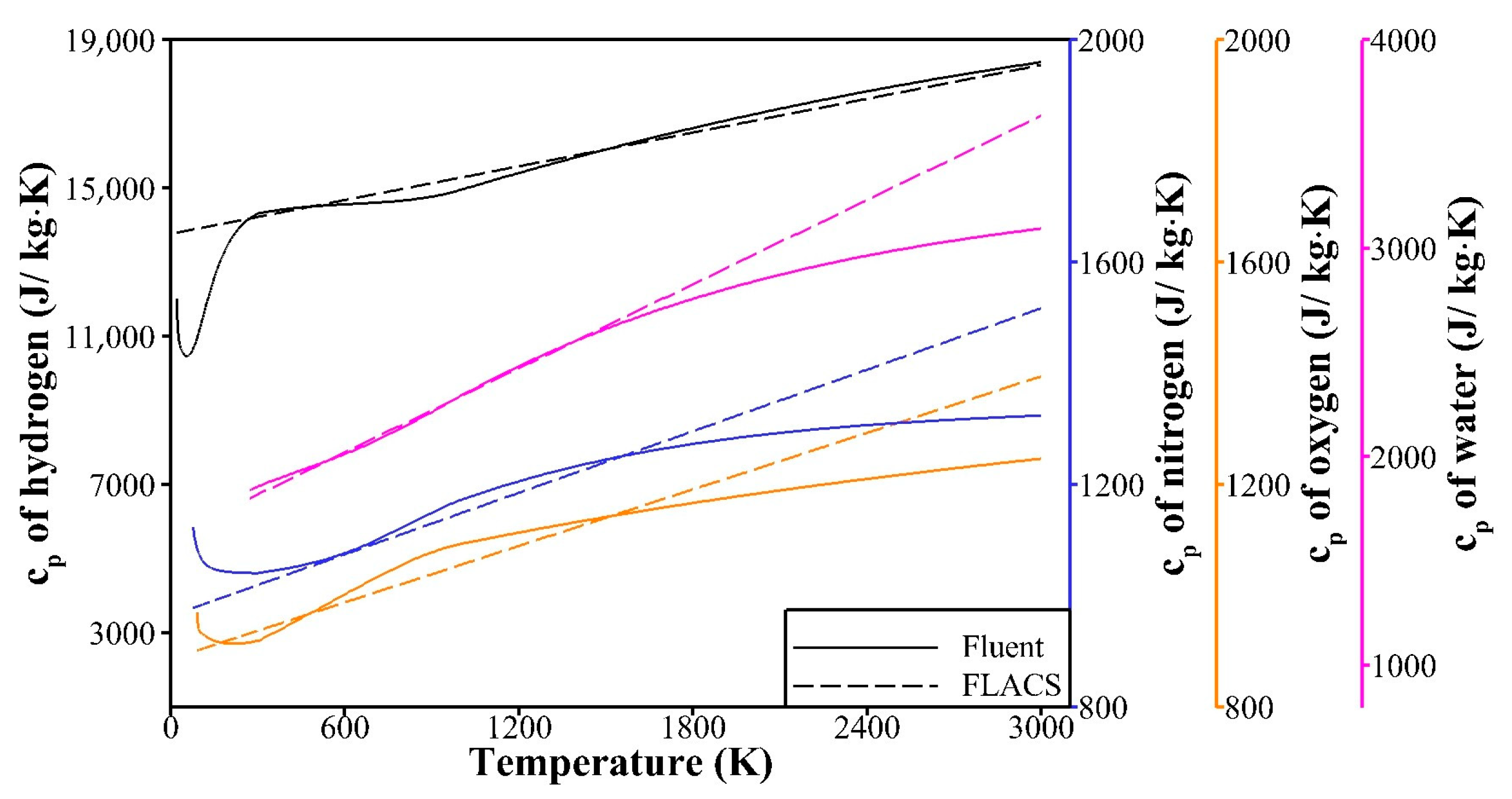
3.1.1. Models of Thermodynamic Properties of Species

The models of thermodynamic properties of species and the liquid–gas mass transfer at hydrogen outlet can impact the entire model performance significantly [28,35,36]. In the two widely used commercial CFD tools, Fluent [15] and FLACS [16], different models of thermodynamic properties and liquid–gas mass transfer are applied. The detailed descriptions of these models are presented as follows.

While the thermodynamics properties of species are calculated by default with piecewise-polynomial functions in Fluent [15], linear functions on temperature are used to estimate these properties in FLACS [16]. The results of calculated specific heats of gaseous hydrogen, nitrogen, oxygen, and water in the two CFD tools are shown in Figure 1. Significant discrepancies are observed, especially for the specific heats of hydrogen and nitrogen below 300 K and of hydrogen, nitrogen, and water above 1500 K. Constant values of 9747.6 J/(kg K) and 9500 J/(kg K) are assigned to the specific heat of liquid hydrogen in Fluent [15] and FLACS [16], respectively.

3.1.2. Model of Liquid–Gas Mass Transfer in Fluent

In Fluent [15], the mixture model is employed to model the flow of the liquid and gaseous hydrogen mixture based on the assumption that the liquid and gaseous hydrogen flow at the same velocity. The mass flow rate at liquid hydrogen outlet is expressed as follows:

$$m_1={\rho }_{mix,1}{v}_{1}A,$$

(6)

where $m_1$ is the mass flow rate at outlet, $v_1$ is the velocity, and $A$ is the outlet area. ${\rho }_{mix,1}$ is the density of the liquid–gas mixture, which is determined by

$${\displaystyle \frac{1}{{\rho }_{mix,1}}}={\displaystyle \frac{q_g}{{\rho }_g}}+{\displaystyle \frac{1-q_g}{{\rho }_l}},$$

(7)

where $q$ represents the mass fraction of hydrogen in different phases. The subscripts $g$ and $l$ represent the gas and liquid phase, respectively.

The mass transfer between liquid and gas phases for a specific species is governed by the Lee model [23].

$${\displaystyle \frac{\partial }{\partial t}}\left({\alpha }_g{\rho }_g\right)+{\displaystyle \frac{\partial }{\partial x_j}}\left({\alpha }_g{\rho }_g{u}_{g,j}\right)=\dot{m_{lg}}-\dot{m_{gl}.}$$

(8)

Here, ${\alpha }_g$ is the volume fraction of the species in gas phase. $u_{g,j}$ is the velocity of the species in gas phase in the $j$ direction. $\dot{m_{lg}}$ and $\dot{m_{gl}}$ represent the mass transfer rate from the liquid to the gas phase due to evaporation and from the gas to the liquid phase due to condensation, respectively. The mass transfer rate $\dot{m_{lg}}$ and $\dot{m_{gl}}$ are jointly determined by the liquid phase temperature $T_l$, gas phase temperature $T_g$, and the saturation temperature $T_{sat}$. When $T_l>T_{sat}$, the evaporation rate is given by

$$\dot{m_{lg}}=c_1{\alpha }_l{\rho }_l{\displaystyle \frac{T_l-T_{sat}}{T_{sat}}}.$$

(9)

When $T_{sat}>T_g$, the condensation rate is

$$\dot{m_{gl}}=c_2{\alpha }_g{\rho }_g{\displaystyle \frac{{T_{sat}-T}_g}{T_{sat}}}.$$

(10)

The symbols $c_1$ and $c_2$ in Equations (9) and (10) are coefficients characterizing the evaporation and condensation rates, respectively.

3.1.3. Model of Liquid–Gas Mass Transfer in FLACS

In FLACS [16], the liquid–gas mass transfer of hydrogen is defined using the pseudo source model. The pseudo source indicates a representative hydrogen outlet, where the liquid hydrogen has evaporated completely [38]. This model simplifies the process of liquid–gas mass transfer by replacing the complex physical source with the pseudo source, assuming that the momentum and energy conservations are achieved along the release direction [38,41]. The pseudo source model was validated in the previous work by Hansen [38], and the results show that it can reproduce the dense gas behavior of liquid hydrogen.

The velocity of the liquid–gas two-phase flow can be calculated by using Equation (6). During the flow process from the release position to the outlet of the pseudo source, the two-phase flow entrains air and absorbs heat. Assuming that all the heat absorbed is used for the evaporation of liquid hydrogen, the required amount of air is estimated by

$$m_{air}={\displaystyle \frac{\left(1-q_g\right)m_1\gamma }{c_p\left(T_{\infty }-T_{sat}\right)}},$$

(11)

where $\gamma$ is the latent heat of the vaporization of liquid hydrogen, $c_p$ is the specific heat of air, and $T_{\mathrm{\infty }}$ is the ambient temperature. Based on the momentum conservation along the release direction, the velocity and the area of the pseudo source are expressed as follows:

$$v_{pseudo}={\displaystyle \frac{m_1{v}_1}{m_1+m_{air}}},$$

(12)

and

$$A_{pseudo}={\displaystyle \frac{\frac{m_1}{{\rho }_g}+\frac{m_{air}}{{\rho }_{air}}}{v_{pseudo}}},$$

(13)

respectively. Thus, the mass flow rate at the outlet of pseudo source is

$$m_2={\rho }_{mix,2}{v}_{pseudo}{A}_{pseudo}.$$

(14)

Here, ${\rho }_{mix,2}$ represents the density of the gas mixture of evaporated liquid hydrogen and entertained air.

3.2. Computational Domain and Boundary Conditions

A computational domain of $\mathrm{50 }\mathrm{m }\times \mathrm{10 }\mathrm{m }\times \mathrm{10 }\mathrm{m}$ is used to simulate the release of liquid hydrogen and is illustrated in Figure 2. The left boundary at X = 0 m serves as the velocity inlet for wind, with air as the inflow species and a wind speed of 2.9 m/s at a height of 2.5 m. The right boundary at X = 50 m represents the outlet with a pressure of 1 bar. The bottom boundary at Z = 0 m represents the ground with a boundary of the stationary wall. The ground is modeled as concrete with a density of 2350 kg/m³, a specific heat of 0.97 kJ/(kg K), a temperature of 284.5 K, and a heat transfer coefficient of 1.28 W/(m K) [23]. Following the recommendation of Fluent [15] and FLACS [16], the front boundary at Y = −5 m, the back at Y = 5 m, and the top at Z = 10 m are set as open boundaries to minimize the influence of boundaries far from the main flow region on simulation results [34]. At these boundaries, the normal component of velocity is set to zero, while zero gradient condition is applied to all other variables. The release position of liquid hydrogen is located 10 m away from the left boundary. A cylinder with a characteristic diameter of 0.0263 m is used to represent the pipeline with a length of 1 m. The right side of the cylinder is set as the mass flow inlet with a coordinate at 11, 0, 0.86.

In this study, air is modeled as a mixture consisting of nitrogen, oxygen, and water vapor, as confirmed by the literature study [30]. The computational domain is initialized with stationary air at 283.5 K. The wind flow exits at the beginning to establish a stable wind field, with the direction perpendicular to the wind velocity inlet boundary. Liquid hydrogen is released at 5 s of the simulation.

When released, liquid hydrogen stored under cryogenic and pressurized conditions undergoes immediate evaporation. Since there is no measured data for the mass fraction of evaporated hydrogen at the outlet in HSL experiments, several studies were conducted to determine the mass fraction at the boundary [30,42]. Houf et al. [42] estimated the mass fraction of gaseous hydrogen at the outlet by using an isentropic model, and validated results against experimental data for gas release at a temperature of 80 K and pressures of 0.825 and 3.2 MPa. Giannissi et al. [30] compared the mass fraction of gaseous hydrogen calculated with the isentropic and isenthalpic assumptions. They revealed that, for liquid hydrogen released at a pressure of 2 bar, the relative deviation between the results of mass fraction at the outlet based on the two assumptions is 11.35%; thus, the impact of the isentropic and isenthalpic assumptions on the simulation results of liquid hydrogen release is negligibly small.

In this study, the mass fraction of gas phase is estimated by assuming an isenthalpic process, as given by

$$q_g={\displaystyle \frac{h_{1l}-h_{2l}}{h_{2g}-h_{2g}}},$$

(15)

where $h_{1l}$ represents the enthalpy of liquid hydrogen at storage conditions. $h_{2l}$ and $h_{2g}$ represent the enthalpies of liquid and gas hydrogen at hydrogen outlet, respectively. The enthalpies of hydrogen at different conditions can be found in the literature [43], and the mass fraction of hydrogen in gas phase is determined as 0.063.

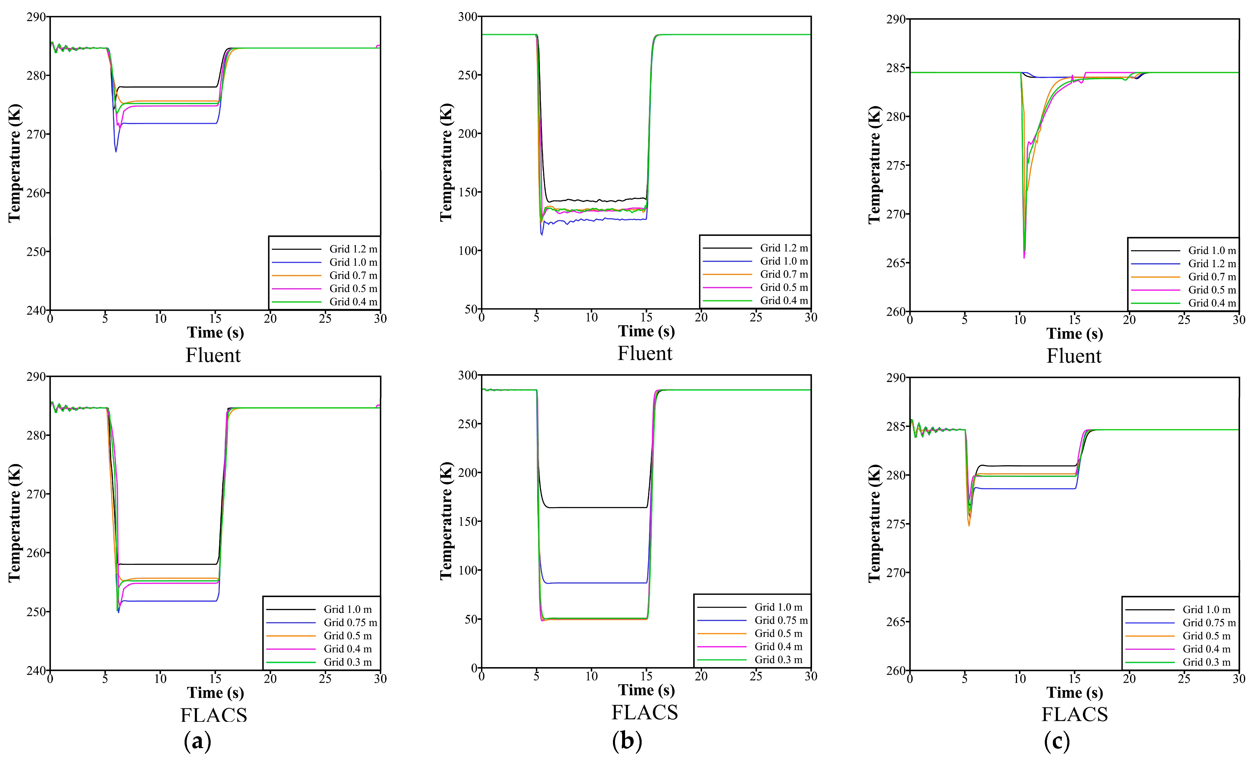
3.3. Mesh Information and Solution Method

Hexahedral meshes are generated in Fluent [15] and FLACS [16]. Local mesh refinement is imposed to those close to the release point and those near the ground. At the release point, the cell dimensions are equal to the release diameter, and near the ground, the smallest dimension of the cell is 0.02 m. Mesh independence tests are performed at all sensor positions for the predicted temperature. The results indicate that the mesh convergence is achieved with a relative error of less than 5% in the temperature prediction, when the global mesh size is smaller than 0.7 m for Fluent [15] and 0.5 m for FLACS [16]. The results of the mesh tests are shown in Figure 3. Therefore, for models developed with Fluent [15] and FLACS [16], mesh sizes of 0.7 m (291666 cells) and 0.5 m (240900 cells) are selected, respectively.

Transient simulations are performed to simulate the release of liquid hydrogen. A fixed time step size of 0.001 s is applied with a convergence criterion of 10⁻⁴ in Fluent [15] and FLACS [16] following the literature recommendation [23].

4. Results and Discussion

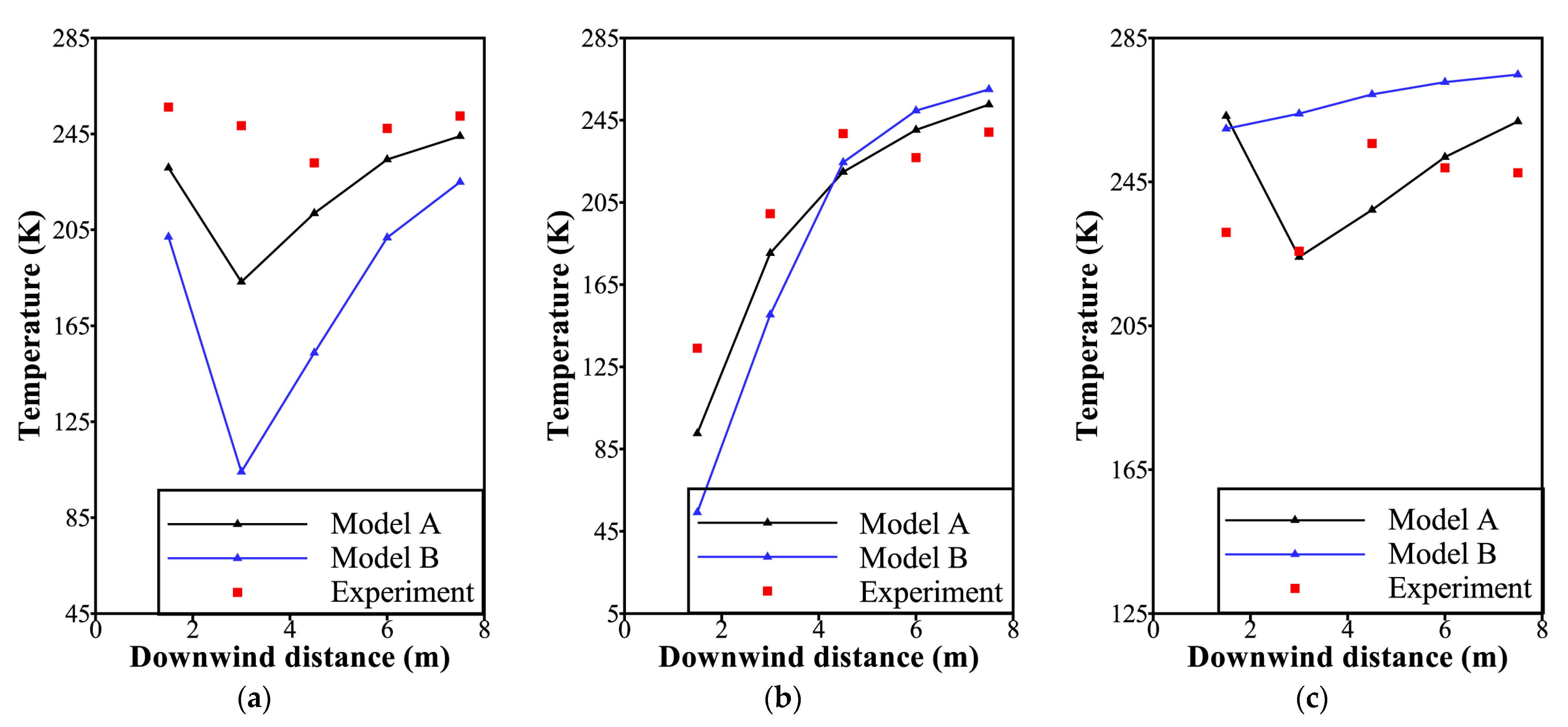
4.1. Model Validation

The models developed with Fluent [15] and FLACS [16] are denoted as models A and B, respectively. They were validated against the HSL experimental data of temperature reported in [28].

Table 3. Configurations for models A and B.

CFD Models	Tools	Sub-Models
		Thermodynamic Properties	Liquid–Gas Mass Transfer
Model A	Fluent	Polynomial	Mixture model
Model B	FLACS	Linear	Pseudo source model

shows the detailed configurations for models A and B in terms of sub-models of thermodynamic properties and liquid–gas mass transfer. In the experiment, the wind field exhibits fluctuations, while the standard $k-ϵ$ turbulence model is utilized in the simulations and the wind is aligned with the direction of the hydrogen jet. In this case of simplification for the wind field, the minimum temperature at the sensors is considered for the model validation following the literature recommendation [28,30]. Figure 4 presents the measured and predicted minimum temperatures at heights of 0.25 m, 0.75 m, and 1.25 m. Both models A and B reproduce the development of temperature in the downwind directions at 0.25 m and 0.75 m. However, they both underpredict the temperatures at a height of 0.25 m. In general, average prediction uncertainties of 8.53% and 20.4% are found for models A and B, respectively.

4.2. Comparison of Model Performance for Temperature and Hydrogen Volume Fraction

Figure 5 presents the comparison of the temperatures and hydrogen volume fractions predicted by models A and B. It is shown in Figure 5a that both models provide similar prediction accuracies for the downwind distance of the cryogenic cloud with a temperature of below 273 K. However, discrepancy exists in the vertical rise height of the cryogenic clouds. While both clouds show a downward trend near the liquid hydrogen outlet, the one simulated by model A shows a more pronounced upward lift at the far field. As illustrated in Figure 5b, the discrepancies in the rise height of clouds are also observed in model predictions of hydrogen volume fractions. Moreover, Figure 5b shows that the downwind distance of the flammable cloud, which is defined as the cloud with a volume fraction of above 4%, predicted by model A is substantially shorter than that predicted by model B. This is primarily attributed to the fact that model A predicts a smaller region of the hydrogen volume fractions between 0.04 and 0.20.

To further compare both models, the deviations between measured and predicted minimum temperatures at heights of 0.25 m, 0.75 m, and 1.25 m are evaluated by using the assessment criteria recommended by Chang et al. [44], which includes the fractional bias (FB), geometric mean bias (MG), and geometric mean variance (VG). FB and MG are measures of mean relative bias, and VG represents mean relative scatter. The corresponding formulas are

$$FB=2{\displaystyle \frac{〈T_o〉-〈T_p〉}{〈T_o〉+〈T_p〉}},$$

(16)

$$MG=exp\langle \mathit{ln}\left({\displaystyle \frac{T_o}{T_p}}\right)\rangle ,$$

(17)

and

$$VG=exp\langle {\left(ln{\displaystyle \frac{T_o}{T_p}}\right)}^2\rangle .$$

(18)

Here, the symbol 〈 〉 represents the average value over the dataset. $T_o$ and $T_p$ refer to the measured and predicted temperature, respectively. According to the definitions, the FB, MG, and VG of a model, whose prediction agrees perfectly with the experimental data, are 0, 1, and 1, respectively. The deviations between the experimental and the predicted minimum temperatures are presented in

Table 4. Deviations between measured and predicted minimum temperatures.

Model	Height	FB	MG	VG
Model A	H = 0.25 m	−0.127	0.879	1.024
	H = 0.75 m	−0.059	0.924	1.012
	H = 1.25 m	0.024	1.024	1.005
	Sum	−0.052	0.940	1.014
Model B	H = 0.25 m	−0.330	0.692	1.231
	H = 0.75 m	−0.101	0.807	1.202
	H = 1.25 m	0.103	1.110	1.012
	Sum	−0.096	0.853	1.144

.

The results show that both models underpredict the temperatures, with the largest difference at 0.25 m. At 1.25 m, both models overestimate the temperatures. As illustrated, model A shows prediction advantages over model B.

As stated above, model A developed with Fluent [15] demonstrates higher prediction accuracy in temperature. And more notably, the significant discrepancies in the prediction results of models A and B under the same liquid hydrogen release scenario suggest a need to further explore the underlying reasons. Previous studies indicate that the entire model performance is highly sensitive to the models of thermodynamic properties and the liquid–gas mass transfer [28,35,36]. The discrepancies in the temperatures and hydrogen volume fractions predicted by the two models developed with Fluent [15] and FLACS [16] can be attributed to the differences between these sub-models. Thus, the impact of models of thermodynamic properties and liquid–gas mass transfer on the prediction results of liquid hydrogen release is explored in the following section.

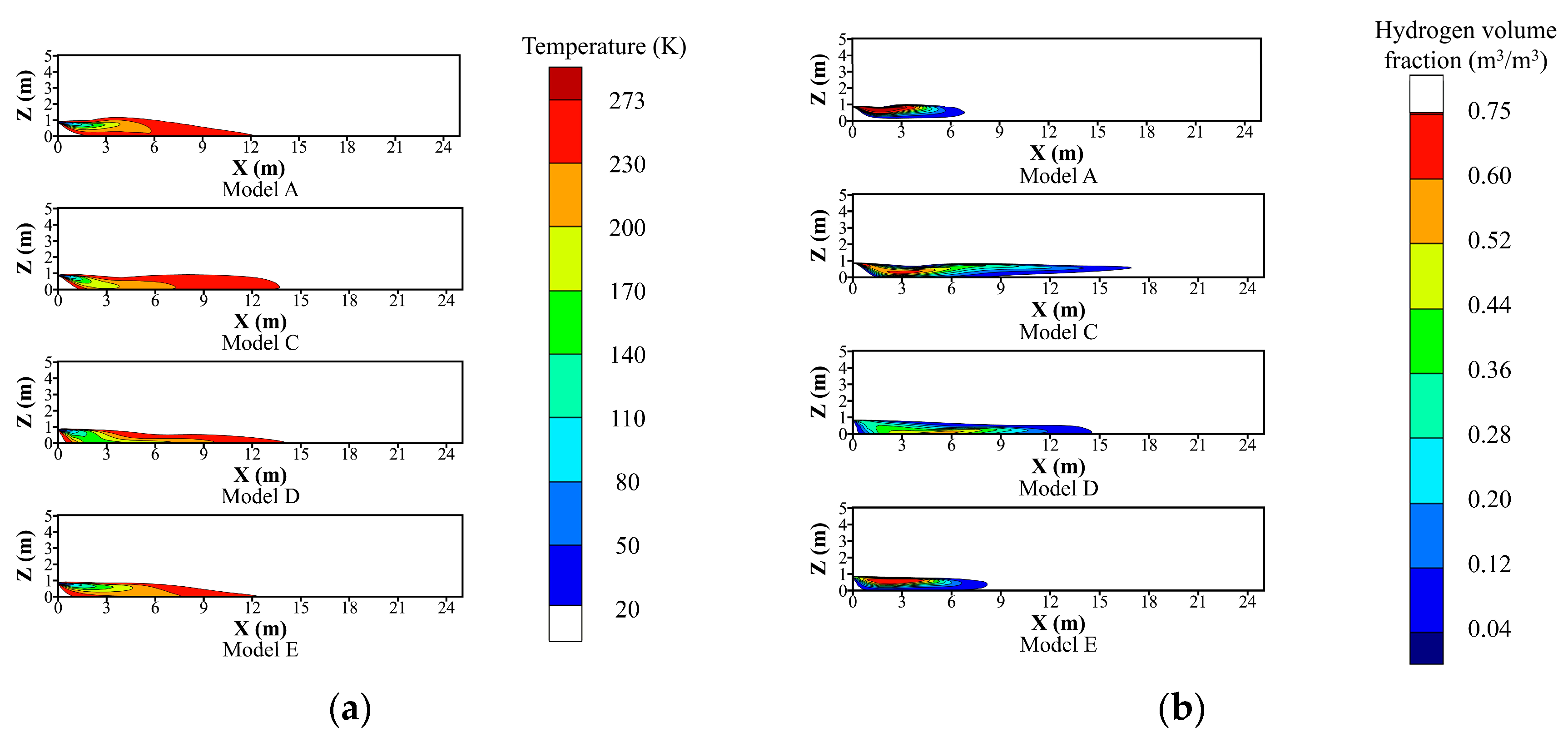
4.3. Impact of Models of Thermodynamic Properties and Liquid–Gas Mass Transfer

The CFD tool Fluent [15] offers a wide range of customizable parameters and enables efficient analyses of the impact of various models on the prediction results [15]. In this study, the FLACS [16] sub-models are incorporated into Fluent [15] and the resulting prediction differences are evaluated for the exploration of the impacts of models of thermodynamic properties and liquid–gas mass transfer. For this, Models C and D are developed by incorporating the FLACS [16] models of thermodynamic properties and liquid–gas mass transfer to Fluent [15], respectively. Model E is developed by incorporating both FLACS [16] sub-models simultaneously. The detailed configurations for models C, D, and E are summarized in

Table 5. Configurations of models C, D, and E.

CFD Models	Tools	Sub-Models
		Thermodynamic Properties	Liquid–Gas Mass Transfer
Model C	Fluent	Linear	Mixture model
Model D	Fluent	Polynomial	Pseudo source model
Model E	Fluent	Linear	Pseudo source model

.

Figure 6 compares the temperatures and hydrogen volume fractions predicted by models A, C, D, and E. As illustrated in Figure 6a, models C, D, and E predict lower temperatures near the ground and at reduced vertical rise heights, compared with model A. It indicates that both FLACS [16] sub-models of thermodynamic properties and liquid–gas mass transfer overestimate the dense effect of clouds. Furthermore, model D underestimates the highest hydrogen volume fraction within the flammable cloud, possibly due to the inclusion of air entrainment in the pseudo source model of FLACS [16], which enhances mixing and hydrogen dilution.

These observations highlight the strong influence of models of thermodynamic properties and liquid–gas mass transfer on the prediction results. Compared to Fluent [15], the models of FLACS [16] lead to underestimations of the vertical rise height and the highest hydrogen volume fraction of the cloud, as clearly demonstrated by the comparison between models A and E shown in Figure 6a,b.

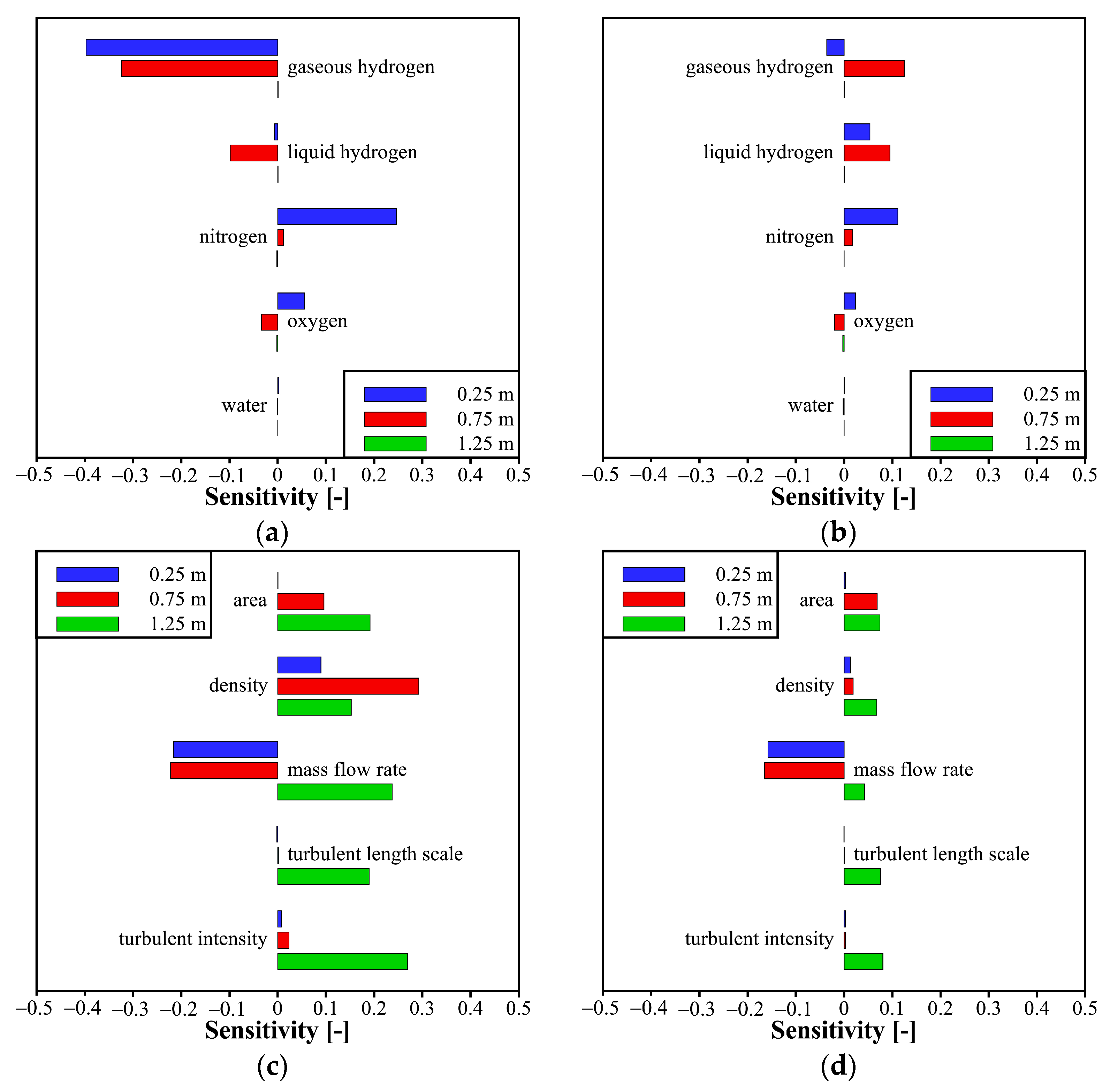
4.4. Sensitivity Analyses of Parameters in Models of Thermodynamic Properties and Liquid–Gas Mass Transfer

Sensitivity analyses are performed to identify the important parameters in the models of thermodynamic properties and liquid–gas mass transfer for temperature prediction. The sensitivity coefficient of parameter $i$ is defined as follows:

$$Sensitivit{y}_i={\displaystyle \frac{A_i}{T_i}}{\displaystyle \frac{\partial T_i}{\partial A_i}},$$

(19)

where $A_i$ is the value of the parameters and $T_i$ is the predicted temperature. Sensitivities are evaluated with respect to the predicted temperatures at different positions. For each height of 0.25 m, 0.75 m, and 1.25 m, both the lowest and highest values of the predicted temperature values are considered at targets of interest of the sensitivity analysis. For example, as illustrated in Figure 6a, at 0.25 m. the lowest and highest temperatures are predicted at 3 m and 7.5 m downwind of the release position, respectively. For parameters in the models of thermodynamic properties, the specific heats of hydrogen, nitrogen, oxygen and water are taken into account. For parameters in the models of liquid–gas mass transfer, sensitivities on the area, density, and mass flow rate at liquid hydrogen outlet are estimated. In addition, the sensitivity on the turbulence parameters of turbulence length scale and turbulence intensity is also examined, due to the fact that they affect the flow development significantly [45].

Figure 7a–d presents the results of the sensitivity analyses. A comparison of Figure 7a,b with Figure 7c,d reveals that temperature predictions at 0.25 m and 0.75 m are more influenced by the specific heats, whereas at 1.25 m, the parameters in mass flow specification have a larger impact. The temperature predictions are highly sensitive to the specific heats of hydrogen and nitrogen and the mass flow rate, while the minimum temperature is also influenced by the density at outlet.

Among these parameters, turbulence has the most significant impact on temperature prediction at 1.25 m, highlighting the necessity of detailed atmospheric turbulence measurements during liquid hydrogen release tests to enhance predictive accuracy for temperature at a relatively elevated height from the ground.

5. Conclusions

In the current study, two computational fluid dynamics models for liquid hydrogen release were developed using the widely used commercial tools Fluent [15] and FLACS [16]. The models were validated using the temperature experimental data in the literature. A comparison of model performance reveals strong discrepancies between their predicted temperatures and hydrogen volume fractions. The model developed with Fluent [15] shows prediction advantages of temperature over the one with FLACS [16]. Further investigation is carried out to explore the impact of models of thermodynamic properties and liquid–gas mass transfer applied in Fluent [15] and FLACS [16] on prediction accuracy. The results indicate that when compared with the Fluent [15] models, the FLACS [16] models of thermodynamic properties and liquid–gas mass transfer underestimate the vertical rise height and the highest hydrogen volume fraction of the cloud. Insights into important parameters affecting the model prediction accuracy are provided by the results of the sensitivity analyses on the parameters in the two sub-models. The specific heats of hydrogen and nitrogen, in conjunction with the mass flow rate and outflow density in the model of the liquid–gas mass transfer, are found to affect model performance significantly. In addition, the requirements of comprehensive data on atmospheric turbulence during liquid hydrogen release are highlighted for model validation.

References

1. Midilli, A.; Ay, M.; Dincer, I.; Rosen, M.A. On hydrogen and hydrogen energy strategies I: Current status and needs. Renew. Sustain. Energy Rev. 2005, 9, 255–271. [Google Scholar] [CrossRef]
2. Aasadnia, M.; Mehrpooya, M. Large-scale liquid hydrogen production methods and approaches: A review. Appl. Energy 2018, 212, 57–83. [Google Scholar] [CrossRef]
3. Sherif, S.A.; Zeytinoglu, N.; Veziroglu, T.N. Liquid hydrogen: Potential, problems, and a proposed research program. Int. J. Hydrogen Energy 1997, 22, 683–688. [Google Scholar] [CrossRef]
4. Najjar, Y.S. Hydrogen safety: The road toward green technology. Int. J. Hydrogen Energy 2013, 38, 10716–10728. [Google Scholar] [CrossRef]
5. Faye, O.; Szpunar, J.; Eduok, U. A critical review on the current technologies for the generation, storage, and transportation of hydrogen. Int. J. Hydrogen Energy 2022, 47, 13771–13802. [Google Scholar] [CrossRef]
6. Kangwanpongpan, T.; Makarov, D.; Cirrone, D.; Molkov, V. LES model of flash-boiling and pressure recovery phenomena during release from large-scale pressurised liquid hydrogen storage tank. Int. J. Hydrogen Energy 2024, 50, 390–405. [Google Scholar] [CrossRef]
7. Lowesmith, B.J.; Hankinson, G.; Chynoweth, S. Safety issues of the liquefaction, storage and transportation of liquid hydrogen: An analysis of incidents and HAZIDS. Int. J. Hydrogen Energy 2014, 39, 20516–20521. [Google Scholar] [CrossRef]
8. Aziz, M. Liquid Hydrogen: A Review on Liquefaction, Storage, Transportation, and Safety. Energies 2021, 14, 5917. [Google Scholar] [CrossRef]
9. Alfarizi, M.G.; Ustolin, F.; Vatn, J.; Yin, S.; Paltrinieri, N. Towards accident prevention on liquid hydrogen: A data-driven approach for releases prediction. Reliab. Eng. Syst. Saf. 2023, 236, 109276. [Google Scholar] [CrossRef]
10. Ikeuba, A.I.; Sonde, C.U.; Charlie, D.; Usibe, B.E.; Raimi, M.; Obike, A.I.; Magu, T.O. A review on exploring the potential of liquid hydrogen as a fuel for a sustainable future. Sust. Chem. One World 2024, 3, 100022. [Google Scholar] [CrossRef]
11. Hall, J.E.; Hooker, P.; Willoughby, D. Ignited releases of liquid hydrogen: Safety considerations of thermal and overpressure effects. Int. J. Hydrogen Energy 2014, 39, 20547–20553. [Google Scholar] [CrossRef]
12. Witcofski, R.D.; Chirivella, J.E. Experimental and analytical analyses of the mechanisms governing the dispersion of flammable clouds formed by liquid hydrogen spills. Int. J. Hydrogen Energy 1984, 9, 425–435. [Google Scholar] [CrossRef]
13. Schmidtchen, U.; Marinescupasoi, L.; Verfondern, K.; Nickel, V.; Sturm, B.; Dienhart, B. Simulation of accidental spills of cryogenic hydrogen in a residential area. Cryogenics 1994, 34, 401–404. [Google Scholar] [CrossRef]
14. Willoughby, D.B.; Royle, M. Experimental releases of liquid hydrogen. In Proceedings of 4th International Conference on Hydrogen Safety, San Francisco, CA, USA, 12–14 September 2011. [Google Scholar]
15. ANSYS Inc. ANSYS Fluent 2022 R1, Theory Guide; ANSYS Inc.: Canonsburg, PA, USA, 2022. [Google Scholar]
16. GexCon. FLACS v21.3 User’s Manual; GexCon: Bergen, Norway, 2021. [Google Scholar]
17. Venetsanos, A.G.; Baraldi, D.; Adams, P.; Heggem, P.S.; Wilkening, H. CFD modelling of hydrogen release, dispersion and combustion for automotive scenarios. J. Loss Prev. Process Ind. 2008, 21, 162–184. [Google Scholar] [CrossRef]
18. Pashchenko, D. Comparative analysis of hydrogen/air combustion CFD-modeling for 3D and 2D computational domain of micro-cylindrical combustor. Int. J. Hydrogen Energy 2017, 42, 29545–29556. [Google Scholar] [CrossRef]
19. Sun, H.J.; Yan, P.H.; Xu, Y.H. Numerical simulation on hydrogen combustion and flow characteristics of a jet-stabilized combustor. Int. J. Hydrogen Energy 2020, 45, 12604–12615. [Google Scholar] [CrossRef]
20. Pu, L.; Shao, X.Y.; Zhang, S.Q.; Lei, G.; Li, Y.Z. Plume dispersion behaviour and hazard identification for large quantities of liquid hydrogen leakage. Asia-Pac. J. Chem. Eng. 2019, 14, e2299. [Google Scholar] [CrossRef]
21. Jin, T.; Liu, Y.L.; Wei, J.J.; Wu, M.X.; Lei, G.; Chen, H.; Lan, Y.Q. Modeling and analysis of the flammable vapor cloud formed by liquid hydrogen spills. Int. J. Hydrogen Energy 2017, 42, 26762–26770. [Google Scholar] [CrossRef]
22. Sklavounos, S.; Rigas, F. Fuel gas dispersion under cryogenic release conditions. Energy Fuels 2005, 19, 2535–2544. [Google Scholar] [CrossRef]
23. Pu, L.; Tang, X.; Shao, X.Y.; Lei, G.; Li, Y.Z. Numerical investigation on the difference of dispersion behavior between cryogenic liquid hydrogen and methane. Int. J. Hydrogen Energy 2019, 44, 22368–22379. [Google Scholar] [CrossRef]
24. Middha, P.; Ichard, M.; Arntzen, B.J. Validation of CFD modelling of LH2 spread and evaporation against large-scale spill experiments. Int. J. Hydrogen Energy 2011, 36, 2620–2627. [Google Scholar] [CrossRef]
25. Shen, Y.H.; Wang, D.; Lv, H.; Zhang, C.M. Dispersion characteristics of large-scale liquid hydrogen spills in a real-world liquid hydrogen refueling station with various releasing and environmental conditions. Renew. Energy 2024, 236, 121327. [Google Scholar] [CrossRef]
26. Hansen, O.R.; Hansen, E.S. CFD-modelling of large-scale LH2 release and explosion experiments. Process Saf. Environ. Prot. 2023, 174, 376–390. [Google Scholar] [CrossRef]
27. Schmidt, D.; Krause, U.; Schmidtchen, U. Numerical simulation of hydrogen gas releases between buildings. Int. J. Hydrogen Energy 1999, 24, 479–488. [Google Scholar] [CrossRef]
28. Ichard, M.; Hansen, O.R.; Middha, P.; Willoughby, D. CFD computations of liquid hydrogen releases. Int. J. Hydrogen Energy 2012, 37, 17380–17389. [Google Scholar] [CrossRef]
29. Sun, R.F.; Pu, L.; Yu, H.S.; Dai, M.H.; Li, Y.Z. Modeling the diffusion of flammable hydrogen cloud under different liquid hydrogen leakage conditions in a hydrogen refueling station. Int. J. Hydrogen Energy 2022, 47, 25849–25863. [Google Scholar] [CrossRef]
30. Giannissi, S.G.; Venetsanos, A.G. Study of key parameters in modeling liquid hydrogen release and dispersion in open environment. Int. J. Hydrogen Energy 2018, 43, 455–467. [Google Scholar] [CrossRef]
31. Holborn, P.G.; Benson, C.M.; Ingram, J.M. Modelling hazardous distances for large-scale liquid hydrogen pool releases. Int. J. Hydrogen Energy 2020, 45, 23851–23871. [Google Scholar] [CrossRef]
32. Liu, Y.L.; Wei, J.J.; Lei, G.; Chen, H.; Lan, Y.Q.; Gao, X.; Wang, T.X.; Jin, T. Spread of hydrogen vapor cloud during continuous liquid hydrogen spills. Cryogenics 2019, 103, 102975. [Google Scholar] [CrossRef]
33. Jin, T.; Wu, M.X.; Liu, Y.L.; Lei, G.; Chen, H.; Lan, Y.Q. CFD modeling and analysis of the influence factors of liquid hydrogen spills in open environment. Int. J. Hydrogen Energy 2017, 42, 732–739. [Google Scholar] [CrossRef]
34. Tang, X.; Pu, L.; Shao, X.Y.; Lei, G.; Li, Y.Z.; Wang, X.K. Dispersion behavior and safety study of liquid hydrogen leakage under different application situations. Int. J. Hydrogen Energy 2020, 45, 31278–31288. [Google Scholar] [CrossRef]
35. Chen, W.; Gao, R.; Sun, J.F.; Lei, Y.F.; Fan, X.L. Modeling of an isolated liquid hydrogen droplet evaporation and combustion. Cryogenics 2018, 96, 151–158. [Google Scholar] [CrossRef]
36. vom Lehn, F.; Cai, L.M.; Pitsch, H. Impact of thermochemistry on optimized kinetic model predictions: Auto-ignition of diethyl ether. Combust. Flame 2019, 210, 454–466. [Google Scholar] [CrossRef]
37. Giannissi, S.G.; Venetsanos, A.G.; Markatos, N.; Bartzis, J.G. CFD modeling of hydrogen dispersion under cryogenic release conditions. Int. J. Hydrogen Energy 2014, 39, 15851–15863. [Google Scholar] [CrossRef]
38. Hansen, O.R. Liquid hydrogen releases show dense gas behavior. Int. J. Hydrogen Energy 2020, 45, 1343–1358. [Google Scholar] [CrossRef]
39. Venetsanos, A.G.; Papanikolaou, E.; Bartzis, J.G. The ADREA-HF CFD code for consequence assessment of hydrogen applications. Int. J. Hydrogen Energy 2010, 35, 3908–3918. [Google Scholar] [CrossRef]
40. Visser, D.C.; Houkema, M.; Siccama, N.B.; Komen, E.M.J. Validation of a FLUENT CFD model for hydrogen distribution in a containment. Nucl. Eng. Des. 2012, 245, 161–171. [Google Scholar] [CrossRef]
41. Yuan, W.H.; Li, J.F.; Zhang, R.P.; Li, X.K.; Xie, J.L.; Chen, J.Y. Numerical investigation of the leakage and explosion scenarios in China’s first liquid hydrogen refueling station. Int. J. Hydrogen Energy 2022, 47, 18786–18798. [Google Scholar] [CrossRef]
42. Houf, W.G.; Winters, W.S. Simulation of high-pressure liquid hydrogen releases. Int. J. Hydrogen Energy 2013, 38, 8092–8099. [Google Scholar] [CrossRef]
43. Eric, W.L.; Ian, H.B.; Marcia, L.H.; Mark, O.M. Thermophysical Properties of Fluid Systems. In NIST Chemistry WebBook, NIST Standard Reference Database Number 69; Linstrom, P.J., Mallard, W.G., Eds.; National Institute of Standards and Technology: Gaithersburg, MD, USA, 2025. [Google Scholar]
44. Chang, J.C.; Hanna, S.R. Air quality model performance evaluation. Meteorol. Atmos. Phys. 2004, 87, 167–196. [Google Scholar] [CrossRef]
45. Zhang, Z.; Zhang, W.; Zhai, Z.J.; Chen, Q.Y. Evaluation of various turbulence models in predicting airflow and turbulence in enclosed environments by CFD: Part 2—Comparison with experimental data from literature. HVAC&R Res. 2007, 13, 871–886. [Google Scholar] [CrossRef]
Figure 1. The specific heats of gaseous hydrogen, nitrogen, oxygen, and water.
Energies 18 03052 g001
Figure 2. Computational domain and boundary conditions.
Energies 18 03052 g002
Figure 3. The results of the mesh tests for temperatures 1 m downwind of the release point: (a) at a height of 0.25 m; (b) at a height of 0.75 m; (c) at a height of 1.25 m.
Energies 18 03052 g003
Figure 4. The measured and predicted minimum temperatures at different heights: (a) at a height of 0.25 m; (b) at a height of 0.75 m; (c) at a height of 1.25 m.
Energies 18 03052 g004
Figure 5. Comparison of temperatures and hydrogen volume fractions predicted by models A and B: (a) temperatures; (b) hydrogen volume fractions.
Energies 18 03052 g005
Figure 6. Comparison of temperatures and hydrogen volume fractions at 4 s after release predicted by models A, C, D, and E: (a) temperature; (b) hydrogen volume fraction.
Energies 18 03052 g006
Figure 7. Sensitivities of temperatures at monitor points on parameters: (a,b) denote sensitivities of minimum and maximum temperatures on parameters of thermodynamic properties, respectively. And (c,d) denote sensitivities of minimum and maximum temperatures on parameters of liquid–gas mass transfer, respectively.
Energies 18 03052 g007