Analysis and Control of Voltage Stability in Offshore Wind Systems Under Small Disturbances

Abstract

This paper proposes an analysis of voltage stability under small disturbances following the integration of an offshore wind farm into a real power system, considering various load and generation scenarios under both normal and post-disturbance conditions. This study utilizes the southern region equivalent system, simulated with Anarede software version 11.7.2, an offshore wind farm with a maximum capacity of 2010 MW. This wind farm is modeled as a PQ bus, operating at partial (50%) and full (100%) generation levels. Three power factor scenarios are examined: resistive, capacitive, and inductive. Submodule 2.3 of the Brazilian National System Operator guidelines states that the base case operating conditions are considered voltage insecurity. Resistive and capacitive power factor operation improved voltage stability margins but resulted in overvoltage on several buses. Conversely, inductive power factor operation led to reduced stability margins and undervoltages at buses near the wind farm. Contingency analysis further revealed stability margins below security limits. Static Var Compensators were installed at critical buses to mitigate these effects, successfully eliminating the initial overvoltage and undervoltage. Modeling as PQ buses does not guarantee stability, making compensators essential for the safe integration of offshore wind generation in Brazilian test systems.

1. Introduction

Brazil’s rise in onshore wind energy has spurred interest in offshore wind energy, which has offered advantages such as lower turbulence and higher wind speeds, leading to significantly increased energy production [1]. Nowadays, China, the United Kingdom, and Germany account for more than 83% of the 55.9 GW of globally installed offshore wind generation [2].

In Brazil, this energy source represents one of the most promising renewable energy technologies, with more than 234 GW in projects under evaluation by IBAMA [3]. This installation’s potential represents less than 25% of Brazil’s overall technical wind capacity, which, according to EPE [4] research, could reach approximately 700 GW at sites with depths up to 50 m. Despite the considerable potential, implementing this type of energy presents challenges related to increased grid penetration levels, such as issues related to voltage and frequency stability [5].

Voltage stability refers to the ability of the power system to maintain adequate voltage levels at all buses after a disturbance [6,7]. In voltage stability studies, the determination of the PV curve is extremely important to calculate the voltage stability margin (VSM), which refers to the maximum system load level that guarantees the existence of a balance point. Different methods have been proposed to calculate and increase the VSM in systems with synchronous generation only and through static analysis. In [8,9], the authors propose the Continuation Power Flow, which requires few operating points to plot the PV curve and determine the maximum power transfer. In [10], the authors apply the Look-Ahead method to quickly plot the VSM with two load increments and define some preventive measures. In [11], the authors determine the VSM of systems with synchronous generation considering variations in the direction of load growth. In [12,13,14], the authors apply artificial intelligence techniques to calculate the VSM, but again, the system only presents synchronous generation. In [15,16], the authors apply physical knowledge with Neural Networks to identify the VSM in a system with synchronous generation. In [17], the authors propose a method based on the Thevenin equivalent model and cubic spline extrapolation technique to identify the VSM of power systems but requires system reduction. In [18], the authors create a new index and evaluate the VSM of systems with Phasor Measurement Units. In [19], the authors apply a metaheuristic called Particle Swarm Optimization to compute the VSM through an optimization model. In [20], the authors propose to use the second-order cone approximation to calculate the VSM. In [21], the authors propose to calculate the VSM considering contingencies using the Pade approximation and holomorphic embedding. In [22], the authors propose an index to calculate the VSM of a system with only synchronous generation using data from the SCADA system and Phasor Measurement Units.

Thus, the scientific community has proposed different and promising techniques to calculate the VSM of power systems with different information. However, these techniques have been proposed, implemented, and evaluated in systems with synchronous generation from thermoelectric and hydroelectric plants. Modern power systems increasingly present alternative generation sources such as wind farms that may present different operating behaviors in relation to synchronous generation sources such as intermittent power generation. Thus, new models and tools must be proposed and evaluated to calculate the VSM and new preventive control strategies may be necessary to increase the VSM when they have inadequate values.

In [23], researchers evaluated the integration of offshore wind energy into the Turkish power system and observed its effects on static voltage stability. The PV curve results demonstrated that the loading margin at the critical bus increased from 50,970 MW to 51,775 MW when the Offshore Wind Power Plant (OWPP) operated at a unity power factor. Activating voltage control further raised the margin to 51,845 MW. Therefore, integrating this source improved the stability margin of the system.

Given the increasing promise of offshore wind power in Brazil for future implementation, and the critical role of voltage stability in power system operation assessment, this paper investigates the connection of an offshore wind farm to the Brazilian electrical grid. The main contribution of this study is the analysis of the impact on steady-state voltage stability under increasing load, N-1 contingency operation, and increased offshore wind generation. Should instability arise, corrective methods will be proposed.

The organization of this paper is as follows. Section 2 presents fundamental concepts of voltage stability and how VSM can be formulated and determined. Section 3 describes the Static Var Compensator as a preventive control strategy for VSM increase. Section 4 describes in detail the Offshore Wind Power Plant modeling applied in this research. Section 5 presents the proposed evaluation methods for voltage stability assessment of the system. Section 6 presents and discusses case studies of voltage stability assessment in the test system with offshore wind integration. Section 7 presents and discusses case studies of voltage control in the test system with appropriate design of Static Var Compensator. Section 8 presents the conclusions of the paper with future research directions.

2. Voltage Stability

Voltage stability is related to the power system’s capacity to maintain the voltage profile on all buses after experiencing a disturbance from a given operating condition [7]. It depends on the system’s ability to maintain and restore the balance between load and generation. A power system becomes voltage-unstable when a disturbance, such as increased demand or altered system conditions, causes a gradual and uncontrollable decrease or increase in voltage at one or more buses. Voltage instability may result in the disconnection of other equipment, the tripping of transmission lines, and load shedding due to the action of the protection system [7,24].

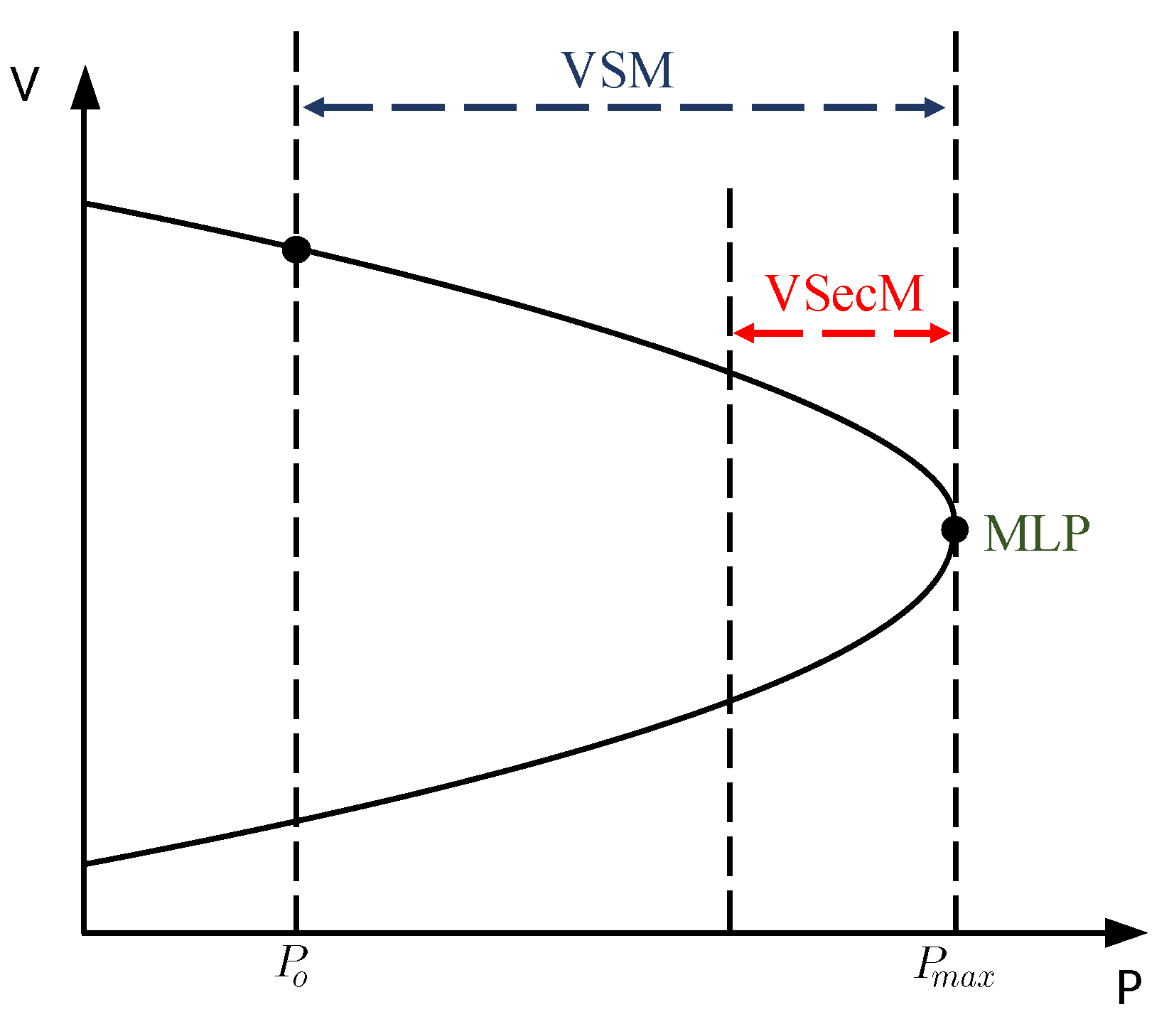
The PV curve (or nose curve) is one parameter utilized in voltage stability analysis, as illustrated in Figure 1. It establishes a correlation between the voltage at a bus and the increase in load under steady-state conditions. The PV curve is obtained through successive solutions of the power flow equations, a process known as Continuous Power Flow (CPF), as the system load level is incrementally increased while maintaining a constant power factor. The resulting equilibrium points define the PV curve [6]. Furthermore, the loads employed in the power flow and CPF studies are modeled as constant power (PQ buses), where power remains independent of voltage magnitude [25,26].

Three quantities can be determined from the PV curve: the VSM, the Voltage Security Margin (VSecM), and the Maximum Loading Point (MLP). The MLP represents the point at which stability is lost and corresponds to the maximum power the network can supply to the load. The VSM, as described in Equation (1), represents the difference between the system’s operating point $\left(P_{\mathrm{o}}\right)$ and the MLP $\left(P_{\max }\right)$. A decrease in the VSM indicates a higher risk of instability within the system. The VSecM, on the other hand, defines the minimum permissible value of the VSM required to maintain system security [27].

$$\mathrm{VSM}=\left({\displaystyle \frac{P_{\max }-P_{\mathrm{o}}}{P_{\mathrm{o}}}}\right)\times 100\%$$

(1)

According to Submodule 2.3 of the Brazilian National System Operator (ONS), Voltage Security Margins for operational planning studies are 7% for the intact system and 4% for the system under N-1 contingency conditions (single element outage). Real-time operation requires a 4% margin. Furthermore, if the system presents situations of voltage instability, i.e., the margin and voltages are not within the pre-established criteria, preventive and/or corrective control actions must be implemented. This can include the deployment of Static Var Compensators to enhance system security [5,6,28].

3. Static Var Compensator

Static Var Compensators (SVCs) have been employed in power systems since the 1970s. Their application extends to both onshore and offshore wind farms, as noted by Ali et al. [5], Gupta [29], and Hamzah et al. [30].

The primary function of SVC is to regulate reactive power compensation to control specific power system parameters, typically bus voltage. It provides flexible and continuous reactive power compensation, operating in capacitive and inductive regions. SVCs can be implemented using switched shunt elements and/or thyristor-controlled reactors and capacitors [26,31]. Figure 2 illustrates typical SVC configurations.

The SVC depicted in Figure 2a consists of a Fixed Capacitor (FC) connected in parallel with a Thyristor-Controlled Reactor (TCR), enabling smooth reactive power control. With the reactor fully conducting, the bank is inductive; conversely, with the reactor fully off, the bank is capacitive. Regulating the reactor current achieves control over the high-voltage bus; the configuration shown in Figure 2b employs a similar principle, which utilizes a Thyristor-Switched Capacitor (TSC) bank [31].

Regarding the optimal placement of SVCs in power systems, Nadeem et al. [32], Gupta [29], and Mehroliya et al. [33] argue that the critical bus, from a voltage stability perspective, is the most suitable candidate for SVC installation. Placement at the critical bus is most effective for increasing the voltage stability margin and maintaining acceptable voltage levels at neighboring buses, pre- and post-contingency.

4. Offshore Wind Power Plant Modeling

In Zhou et al. [34], the offshore wind farm (OWF) is modeled as an equivalent generator and represented as a PQ bus. Similarly, Dabbabi et al. [35] modeled the wind turbines and offshore substation transformers (66 kV/220 kV) as PQ nodes. A final transformer (220 kV/380 kV) is included on the onshore grid to step up the voltage for direct injection into the grid. Dakic et al. [36] also represented the offshore wind farm as a PQ bus in power flow formulation. Furthermore, the Type-3 and Type-4 wind turbines employed in the OWF are also modeled as PQ buses [5,37,38,39].

Therefore, based on the above-mentioned references, the OWF in this study will be modeled as a PQ bus. This modeling approach is referred to as the power factor (PF) control mode. Wind turbines typically operate at a unity PF, indicating zero reactive power generation. However, other values can be specified according to the requirements established by the system operator [38,40] or through optimization strategies, as proposed by Silva et al. [41].

Table 1. PF capacitive and inductive for different countries [42].

	Power Factors
Countries	Capacitive	Inductive
China	0.97	0.97
United Kingdom	0.95	0.95
Germany	0.95	0.95

presents the typical power factor values adopted in countries with offshore wind generation.

This study focuses on steady-state voltage stability assessment using CPF analysis; thus, the PQ model was adopted for its simplicity and widespread use. However, this approach does not consider dynamic aspects and reactive power control, which are relevant under real operating conditions, as discussed by Lu and Rao [43], Huu [44], and Wang et al. [45].

5. Methods

In order to assess voltage stability in offshore wind power systems, the equivalent Brazilian system was determined, along with the potential of a real wind farm and wind integration scenarios. Additionally, Submodule 2.3 of ONS was employed to perform the stability analyses.

5.1. Brazilian Equivalent Test System

The system selected for the analyses in this work is the Reduced Southern System, developed by Alves [46], as illustrated in Figure 3. This system consists of 33 buses, 7 large generating units, 26 transmission lines, and 24 transformers, with a total load demand of 5085 MW and a total generation capacity of 8912 MW. It is divided into two geographical areas, A and B, interconnected by two transmission lines and one transformer. Area A operates near its generation capacity limit, while Area B has a generation surplus, resulting in power flow from B to A.

The Anarede software version 11.7.2, was developed by the Center for Electric Energy Research (CEPEL). Anarede is the most widely used power system analysis software in the Brazilian electric power sector due to its high reliability [47]. For the CPF simulations, several controls were activated, including reactive power limits for PV and slack buses, remote voltage control through generator excitation, and voltage control via automatic transformer tap changing. The ONS typically employs these controls in real operation.

The load increase was implemented in 0.2% increments of both active and reactive power for the two areas (A and B) within the system. This maintains a constant power factor for the load, consistent with the PQ bus modeling specified by ONS Submodule 2.3. The code responsible for balancing active power across all generator buses was also applied in the event of a power imbalance, with a 100% participation factor for all system generators.

5.2. Potential of a Real Offshore Wind Farm

Regarding the potential of a real wind farm to be utilized, IBAMA provides maps of offshore wind projects in the licensing process for future installation. Based on this, and considering the system’s equivalence to the southern region, the project named RS-14, with a capacity to generate 2010 MW, was selected, as shown in Figure 4. This project consists of 134 wind turbines, each with a 15 MW capacity. It was selected among other projects with different capacities because its potential closely aligns with the installed capacity of onshore wind generation in southern Brazil, which is 2026 MW according to data provided by ONS [48].

5.3. Wind Power Insertion Scenarios

Only two onshore substation transformers are considered for wind power integration, as XLPE cable sizing is outside the scope of this research. Concerning the bus selected for wind power injection, Adetokun et al. [49] and Du et al. [50] allocated wind generation to the system’s critical buses from a voltage stability perspective. For that reason, in this study, the critical bus of the Reduced Southern System will be selected as the candidate for offshore wind integration. Specifically, a new PQ bus, representing the offshore wind farm, designated as bus 1, will be connected to the critical bus through two transformers.

Figure 5 illustrates the wind power integration scenarios. As explained in Section 4, the PF control mode permits a range of values from 0.95 capacitive to 0.95 inductive. This range is commonly observed in countries with offshore wind generation. Therefore, three PFs will be considered for subsequent analysis. Furthermore, two-generation scenarios were considered: one with 50% and another with 100% of the wind farm’s available capacity.

6. Voltage Stability Analysis with Offshore Wind Integration

This section presents the simulation results about the impact of an offshore wind farm on voltage stability in the Reduced Southern System.

6.1. Base Case

With the execution of the CPF for the base case, the VSM was 18.8078%, which is within the value established by the ONS for the complete system. Figure 6 presents the PV curves for buses 959 and 895, which exhibited similar behavior, reaching the MLP with voltages of 0.819 p.u. and 0.823 p.u., respectively. These were identified as the system’s critical buses (CBs), i.e., those experiencing the most significant voltage drops at the MLP. Therefore, as described in Section 5.3, bus 959 was selected for OWF integration.

Moreover, the voltage values at the MLP are outside the limits established by ONS. Since both buses have a base voltage of 500 kV, the values should be within the Operational Voltage Range (OVR) of 1.0 to 1.10 p.u., indicating non-compliance. Voltages below this range represent inadequate load supply and may damage equipment due to the low voltage levels, combined with activating undervoltage relays.

• N-1 Criterion

Under the N-1 contingency criterion, buses 959 and 976 were most frequently identified as the critical buses, exhibiting the lowest voltages at the MLP. Similar to the base case, all critical bus voltages are outside the limits established by ONS for the incomplete network.

ONS Submodule 2.3 stipulates a minimum voltage stability margin of 4% for the incomplete network. However, the analysis of

Table 2. Main VSM for different contingencies, along with the corresponding CB values and voltages of CB (pu).

Contingency	VSM (%)	CB	Voltage of CB (pu)
18	0.9125	976	0.7786
7	3.1750	976	0.8670
22	3.6438	976	0.7726
24	4.8188	959	0.8534
12	12.3125	959	0.8168
17	12.8313	938	0.7956

establishes that when disconnecting the circuits of lines 955-964 (contingency 18), 856-933 (contingency 7), and 959-895 (contingency 22), the stability margins are below the limit established by grid procedures. These outaged lines, exhibiting the lowest margins, are located in Area A, which experiences excess demand, leading to undervoltages at neighboring buses. Contingencies 22 and 18 resulted in the lowest voltages among all analyzed outage cases, indicating system instability under these conditions.

In contingencies 24 (line 995-1060), 12 (line 933-955), and 17 (line 938-959), despite having acceptable margins, the voltages at the MLP are below the voltage criteria for outages, where the OVR should range between 0.95 to 1.10 p.u. for 500 kV systems. In these cases, besides the location of these lines in Area A, which exhibits excess demand, the critical buses have significant associated loads, causing the voltage drops.

Finally, it is important to note that some cases involving transmission lines and transformer outages did not converge for the base case, meaning that a power flow solution could not be obtained, as shown in

Table 3. Non-converged contingency cases resulting from line or transformer disconnections.

Disconnected lines	Operational situation
896-897	Non-convergent
933-895	Non-convergent
933-959	Non-convergent
938-955	Non-convergent
964-976	Non-convergent
976-995	Non-convergent
1060-897	Non-convergent
Disconnected transformers	Operational situation
800-824	Non-convergent
2458-896	Non-convergent

. Consequently, these contingencies will be excluded from the stability analysis with the offshore wind farm integration, as their lack of data prevents any meaningful stability evaluation.

6.2. Resistive

The VSM rose to 28.6625% in Scenario 1 after wind power was integrated. In Scenario 2, a slight improvement was observed, with the VSM reaching 31.075%. Both stability margins exceed the ONS requirements. Therefore, the integration of wind power significantly increased the stability margins compared to the base case

Figure 7 illustrates the evolution of the curves for the base case and with the integration of 100% generation at buses 959 and 976, with bus 976 identified as the critical bus in both scenarios. Initial overvoltages are observed at both buses compared to the base case. Notably, these overvoltages also occur at several 500 kV buses in Area A, including bus 1, which corresponds to the wind farm. Overvoltages are undesirable as they may lead to equipment damage or failure due to exceeding insulation capabilities.

• N-1 Criterion

Table 4. Cases with convergence problems for Scenarios 1 and 2.

Contingency	Base (%)	Scenario 1 (%)	Scenario 2 (%)
18	0.9125	Non-convergent	Non-convergent
7	3.1750	Non-convergent	25.1375
22	3.6438	Non-convergent	Non-convergent
24	4.8188	Non-convergent	Non-convergent
12	12.3125	Non-convergent	Non-convergent
17	12.8313	Non-convergent	Non-convergent
29	17.4313	28.2488	Non-convergent
30	12.4438	21.4727	Non-convergent
31	14.6313	24.3594	Non-convergent
33	18.7	28.2488	Non-convergent

compares the stability margins for the two integration scenarios for the N-1 criterion. In some contingencies, convergence was not achieved, preventing system stability assessment. This lack of convergence is attributed to the activation of the reactive power control of the generators, reflecting expected behavior in real power systems. Deactivating this control would lead to pre-contingency reactive power absorption outside operational limits, compromising the validity of the results.

Contingencies 29, 30, 31, and 33 represent the disconnection of generators 810, 904, 915, and 925, respectively. In Scenario 1, before the CPF execution, post-contingency voltages increased compared to pre-contingency values due to the disconnected generators’ loss of reactive power absorption.

Stability margins were substantially higher during CPF execution than in the base case, demonstrating increased system loadability under outage conditions. Figure 8 presents the evolution of contingency 31 for both the base case and the first wind integration scenario at bus 976, as this bus is critical in almost all outages.

Following wind integration, the discontinuities observed in the PV curves in Figure 8 result from generators attempting to regain voltage control during the Continuation Power Flow solution process, specifically due to the automatic back-off mechanism, which influences the construction of curves.

6.3. Capacitive

Scenario 3 demonstrates greater system loadability than Scenarios 1 and 2, achieving a VSM of 33.5609%, which remains above the 7% minimum value established by the ONS. However, in Scenario 4, the power flow analysis did not converge due to excessive reactive power injection. Convergence would only be possible if the generator’s reactive power control were deactivated, similar to the first two scenarios.

Figure 9 shows the evolution of the PV curves at buses 959 and 976 (the critical bus in Scenario 3) for the base case and Scenarios 2 and 3. This figure reveals even higher initial overvoltages compared to Scenario 2. Similar to the previous scenario, these overvoltages are observed at numerous buses in Area A. This operating point is highly undesirable due to the detrimental effects of overvoltages, caused by reactive power injection leading to voltage increases at adjacent buses.

Furthermore, the deformations in the curves for Scenario 3 intensified, indicating that the generators, besides reaching their reactive power absorption limits, require a more significant load increase to regain and maintain voltage control, rendering system operation unacceptable.

• N-1 Criterion

Contingency analysis revealed seven cases of non-convergence, as shown in

Table 5. Cases with convergence problems for Scenario 3.

Contingency	Base (%)	Scenario 3
18	0.9125	Non-convergent
22	3.6438	Non-convergent
30	12.45	Non-convergent
31	14.6375	Non-convergent
28	17.4625	Non-convergent
33	18.6844	Non-convergent
29	18.7719	Non-convergent

. This is consistent with the behavior observed in Scenarios 1 and 2 (non-convergence due to reactive power control activation). In generation outages, excess system reactive power was a primary contributing factor to non-convergence. While three of the seven contingencies did not converge in Scenario 2, this number increased to five in the present analysis. Contingency 27 resulted in system islanding, while contingency 32 consistently supplied reactive power to the system. Consequently, system stability cannot be assessed for these contingencies. Such situations are undesirable from an operational standpoint, particularly because many of these contingencies were classified as critical in the base system.

Table 6. Contingencies with margin reduction for Scenario 3.

Contingency	Base (%)	Scenario 3 (%)	CB (%)	CB Voltage (pu)
7	3.1750	2.6375	840	0.955
12	12.312	5.2188	840	0.952
17	12.8313	2.1375	840	0.952
24	4.8250	0.1313	840	0.952

lists the contingencies that converged but with a lower VSM compared to the base case. Contingencies 7 (line 856-933), 17 (line 938-959), and 24 (line 995-1060) registered values below 4%, thus characterizing voltage instability for these outages.

Also, in Table 6, the critical bus is 840, which differs from the critical buses for the base case contingencies. This bus has a voltage controlled by a transformer tap changer, and the voltage at the MLP is within the permissible voltage range, consistent with the base case value. To illustrate the VSM reduction, Figure 10 shows the PV curves for contingencies 7 and 17 at bus 959.

Contingencies 7 and 24 represent interconnections between Areas A and B. Following wind integration, reactive power flows between these interconnections increased significantly from Area A to B. In other words, Area A has excess reactive power due to the wind farm integration. These factors contribute to margin reduction because, upon disconnection of one of these lines, redispatch occurs, causing more losses and loading in the other lines that interconnect the areas.

Conversely, contingency 17 represents the connection between the bus hosting the wind farm (959) and an auxiliary bus (938), which supplies a large load through three transformers. This contingency becomes critical due to the interrupted power supply to this load, resulting in redistribution to the auxiliary line (955-938); this latter line did not converge for the base case. Furthermore, the other outages resulted in margins above 4%.

6.4. Inductive

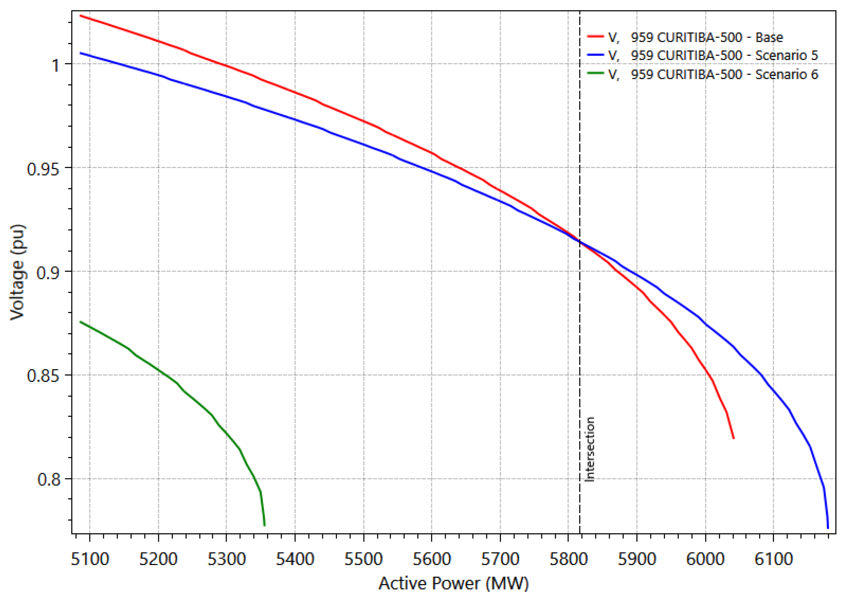
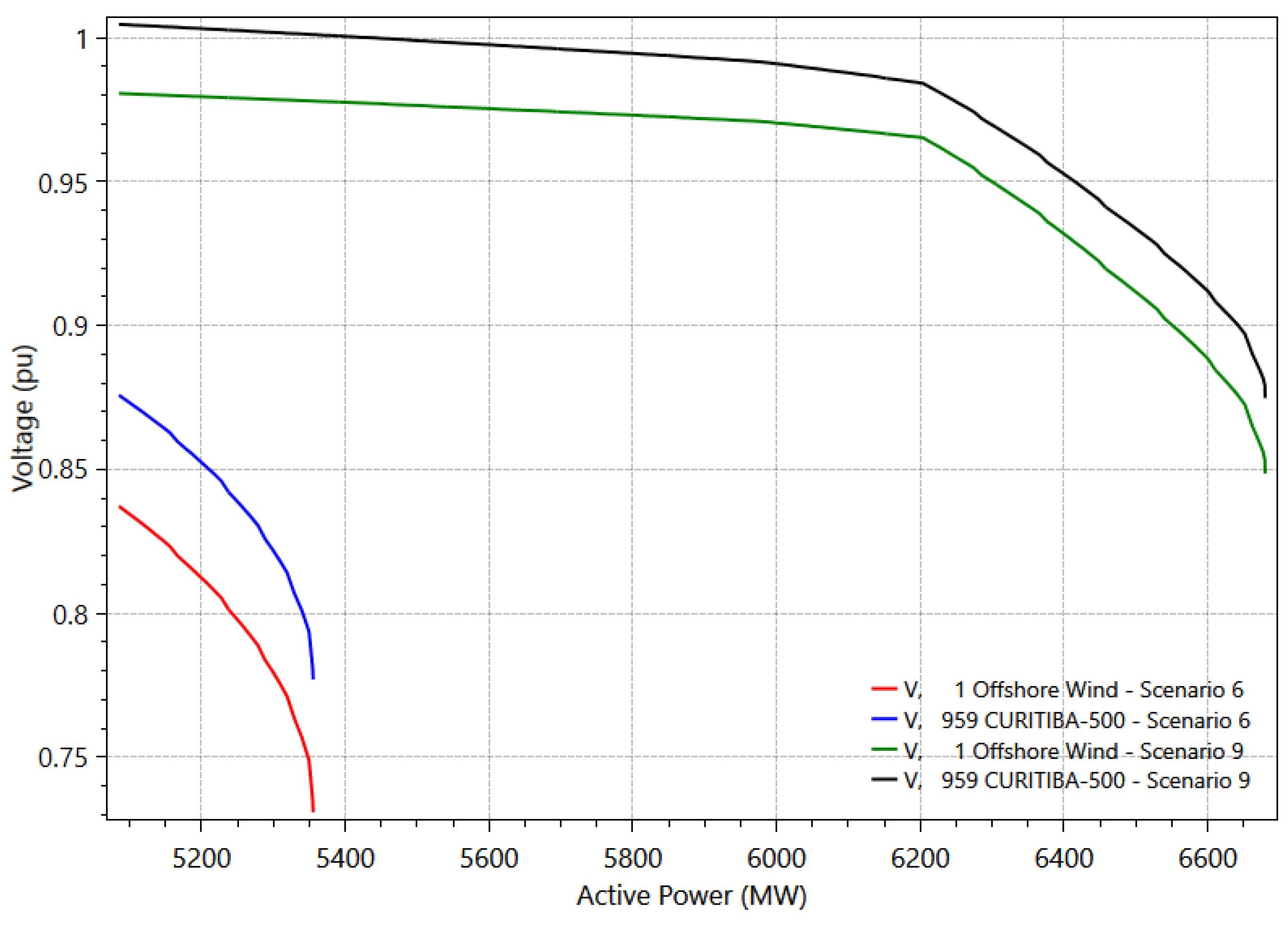
In Scenario 5, the load increase is less than in previous scenarios, reaching a margin of 21.5156%, close to the base case value. In Scenario 6, the load increase is even smaller, reaching only 5.3141%, indicating voltage instability due to high reactive power consumption.

Buses 959 and 1 (OWF) are the most critical in Scenario 6. Figure 11 compares bus 959 in both integration scenarios. In Scenario 5, voltages are lower than the base case during the load increase. However, the voltage profile increases after the intersection of the two curves. In Scenario 6, voltages are significantly lower throughout the load increase, reaching the MLP at 0.777 p.u. These undervoltages are also observed at several buses near the wind farm due to the farm’s high reactive power consumption.

• N-1 Criterion

Table 7. Cases with convergence problems for Scenario 6.

Contingency	Base (%)	Scenario 5 (%)	Scenario 6 (%)
18	0.9125	1.15	Non-convergent
7	3.1750	11.0121	Non-convergent
22	3.6438	4.9456	Non-convergent
24	4.8250	6.5296	Non-convergent
25	12.1063	15.6234	Non-convergent
12	12.3125	13.1404	Non-convergent
17	12.8313	11.9127	Non-convergent
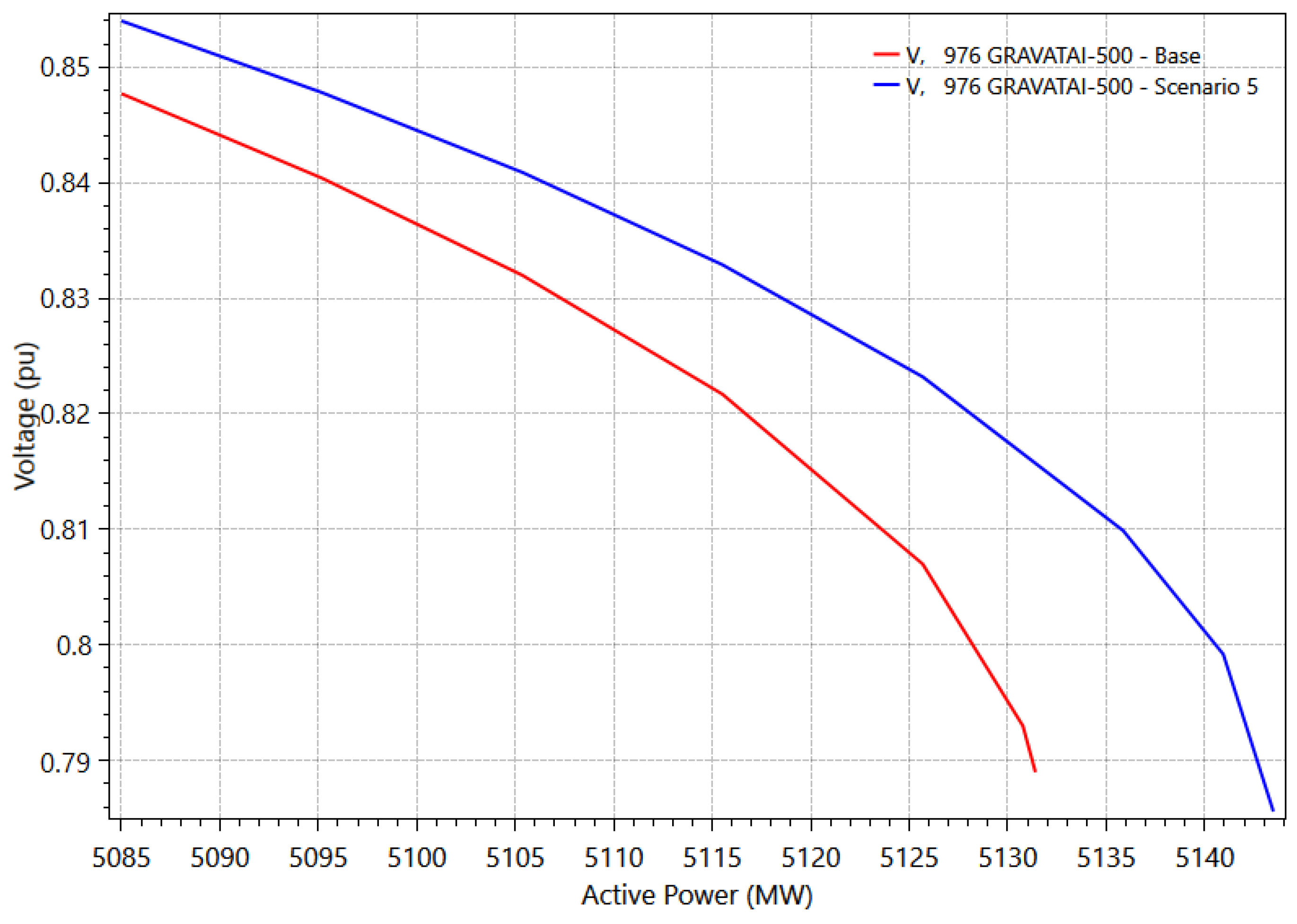
19	15.5875	16.3959	Non-convergent

shows the cases in which convergence problems occurred for Scenario 6, precluding stability analysis in relation to the N-1 criterion. This issue arises from the high reactive power absorption by the OWF. In particular, only one convergent operating point exists, corresponding to a consumption of 361 MVAr—greater than the -601 MVAr adopted for this scenario. This high consumption disrupts the system power balance, preventing convergence. In contrast, in Scenario 5, contingencies 7 (line 856-933), 22 (line 995-964), and 24 (line 995-1060) showed significant margin increases compared to the base case, except for contingency 18 (line 955-964), which exhibited minimal improvement.

Figure 12 shows the PV curve at bus 976, which remained the critical bus in Scenario 5 for contingency 18. This figure reveals slightly higher voltages during the load increase for this scenario; the contingency still leads to voltage instability. Furthermore, this contingency did not converge in Scenarios 1, 2, and 3 compared to previous ones. Contingency 7 exhibited a reduced margin compared to Scenario 2 (from 25.1375% to 11.0121%) and did not converge in Scenario 3.

In Scenario 3, contingencies 7 (line 856-933), 12 (line 933-955), 17 (line 938-959), and 24 (line 995-1060) exhibited increased VSM values, remaining within the safety margin required for proper system operation. Contingencies 7 and 24 are of particular interest, as in Scenario 5, with the wind power integration, Area A no longer exhibited excess reactive power, resulting in a decreased reactive power exchange between areas.

Finally, for the contingencies that converged in Scenario 6, seven cases exhibited VSM values below the acceptable safety margin, indicating voltage instability, as shown in

Table 8. Contingency cases with margins below 4% in Scenario 6.

Contingency	Base (%)	Scenario 5 (%)	Scenario 6 (%)
43	15.9063	17.4298	0.1250
44	15.9188	17.4486	0.1437
34	17.2628	19.4987	2.7090
35	17.3188	19.5540	3.7840
8	16.8	20.5040	2.0465
23	16.9625	19.8415	2.7152
31	14.6313	17.4048	3.7304

.

Contingencies 43 and 44 represent the interconnection between a large load bus (960) and the bus hosting the wind farm (959) via two transformers in parallel. This is similar to contingencies 34 and 35, which connect buses 814 and 895.

One factor contributing to the reduced VSM in these cases is the proximity of the outages to the wind farm. In this integration scenario, the wind farm consumes a significant amount of reactive power, resulting in greater undervoltages at neighboring buses following the outages. Additionally, undervoltages were observed after contingencies 8 (line 856-1060), 23 (line 995-1030), and 31 (generator 915), further contributing to the VSM reduction.

7. Voltage Control by SVC

Given overvoltage, undervoltage instances, and margins below the ONS recommendations, this section presents the results of voltage stability analysis using SVCs. As described in Section 3, SVCs were placed at the system’s critical buses in all integration scenarios: 1, 959, and 976. Additionally, an SVC was placed at bus 995, connected to generator 904, which exhibited high reactive power consumption in the first two scenarios.

Therefore, Section 7.1, Section 7.2 and Section 7.3, along with their respective subsections, explore voltage stability for the three worst-performing integration scenarios, Scenarios 2, 3, and 6, under the N-1 criterion. With voltage control applied, these scenarios are renamed 7, 8, and 9. The SVCs were configured to maintain a voltage of 1.0 p.u. at bus 1 and 1.020 p.u. at the other buses, consistent with ONS recommendations for 230 kV and 500 kV buses.

7.1. Scenario 7

The initial overvoltages that also occurred in several 500 kV buses due to their location in area A were eliminated by the static compensator, which regulated the voltages in the four buses of the system. This operating point is highly desirable, ensuring that equipment insulation limits are not exceeded and voltages remain within the permissible range established by the ONS.

The VSM for this scenario is 47.6891%, exceeding that of Scenario 2 (31.0750%). This indicates that, in addition to a VSM above the 7% requirement of Submodule 2.3, the initial voltages are within the permissible range. Figure 13 illustrates buses 959 and 976, identified as critical for the base case and Scenario 2, respectively, with and without voltage control. The figure shows that the SVCs maintain nearly constant voltage throughout most the load increases.

• N-1 Criterion

In Scenario 2, numerous contingencies initially exhibited convergence failures. However, with the application of SVCs, convergence was achieved in all cases due to the SVCs’ ability to balance system power. This includes generation contingencies (29, 30, 31, and 33), as the SVCs absorbed excess reactive power from the generators, facilitating convergence following the outages and resulting in increased stability margins, as shown in

Table 9. Contingency cases with convergence issues resolved in Scenario 7.

Contingency	Base (%)	Scenario 2 (%)	Scenario 7 (%)
18	0.9125	Non-convergent	13.9592
7	3.1750	25.1375	13.9592
22	3.6438	Non-convergent	22.7192
24	4.8188	Non-convergent	32.7730
12	12.3125	Non-convergent	37.6748
17	12.8313	Non-convergent	22.9754
29	17.4313	Non-convergent	47.5537
30	12.4438	Non-convergent	41.4080
31	14.6313	Non-convergent	44.0640
33	18.7	Non-convergent	47.5629

.

Moreover, Figure 14 compares the PV curves for contingencies 18 (line 955-964) and 22 (line 995-964) at critical bus 976, for both the base case and Scenario 7. This figure demonstrates that, even during the outages, voltages remain close to the control value (1.02 p.u.). Considering the voltage criterion for the reduced system (0.95 to 1.10 p.u.) at the 500 kV buses, the VSM would remain high for both contingencies, increasing system stability and security. Finally, the remaining outages exhibited acceptable margins, without initial voltage violations.

7.2. Scenario 8

Similar to Scenario 7, the initial overvoltages with the capacitive power factor were significantly reduced by the static compensator. However, the resulting voltages were higher compared to the previous scenario. Nevertheless, all bus voltages are within the permissible range, characterizing a desirable system operating point.

Regarding voltage stability, the load increase in Scenario 8 is less than in Scenario 7, reaching a VSM of 45.9317%. This reduced VSM is attributed to the lower power generation (1005 MW), which limits power transfer capability. The critical bus for this scenario remains bus 976, consistent with Scenarios 1, 2, and 3. Figure 15 compares the PV curves for buses 959 and 976 in Scenarios 3 and 8.

As shown in Figure 15, and similar to the previous scenario, voltages remain nearly constant throughout most of the loading process, demonstrating the effectiveness of the control in the scenario with the most voltage violations.

• N-1 Criterion

For the contingency analysis, as in the previous scenario, all contingencies converged with the static reactive compensator in operation. In this scenario, all outages, whether generation, line, or transformer outages, converged and exhibited voltages and margins well above those stipulated for the reduced system, according to grid procedures.

Table 10. Evolution of margins for all contingencies in Scenario 3.

Contingency	Base (%)	Scenario 3 (%)	Scenario 8 (%)
18	0.9125	Non-convergent	13.9404
22	3.6438	Non-convergent	21.5602
30	12.45	Non-convergent	38.3400
31	14.6375	Non-convergent	42.1509
28	17.4625	Non-convergent	45.7864
33	18.6844	Non-convergent	45.8065
29	18.7719	Non-convergent	45.5286
7	3.1750	2.6375	31.4077
24	4.8188	0.1313	33.7507
17	12.8313	2.1375	24.3969
12	12.312	5.2188	37.5936

presents the margin improvements for all contingencies, comparing the base case and Scenario 3. Contingencies 7 and 24, representing interconnections between areas, demonstrate significant margin improvements compared to Scenario 3.

According to Table 10, the critical bus for the five most severe contingencies is 976, except for contingency 17, where the critical bus remains 938. Figure 16 illustrates the increased VSM by comparing the PV curves for contingency 7 at bus 976 in Scenarios 3 and 8.

7.3. Scenario 9

Scenario 6 previously exhibited undervoltages at buses near the wind farm due to its reactive power consumption. However, with SVC deployment, which aims to maintain voltage stability, the controller automatically injects reactive power, raising voltage levels to acceptable operating values.

In Scenario 9, the load increase is less than in Scenarios 7 and 8, reaching a margin of 31.3578%. This VSM value is higher than that observed in Scenario 6 (5.3141%). Thus, the system no longer exhibits voltage instability with the SVC regulation. Figure 17 depicts the PV curves for buses 1 and 959, which remain the most critical, compared to Scenario 6.

• N-1 Criterion

Regarding the N-1 criterion for Scenario 9, all contingencies converged, as the static compensators injected reactive power, establishing a stable operating point. As detailed in Section 6.4, convergence requires a minimum reactive power absorption of 361 MVAr, a value at which power balance is maintained by the compensators. Furthermore, all VSMs remained within acceptable limits.

Table 11. All contingencies after correction in Scenario 6.

Contingency	Base (%)	Scenario 6 (%)	Scenario 9 (%)
18	0.9125	Non-convergent	13.1904
7	3.1750	Non-convergent	26.4184
22	3.6438	Non-convergent	16.6834
24	4.8250	Non-convergent	13.5217
25	12.1063	Non-convergent	26.8416
12	12.3125	Non-convergent	19.5575
17	12.8313	Non-convergent	11.1565
19	15.5875	Non-convergent	16.1646
31	14.6313	3.7304	29.0488
43	15.9063	0.1250	25.6684
44	15.9188	0.1437	25.6996
8	16.8	2.0465	29.9327
23	16.9625	2.7152	29.4925
34	17.2628	2.7090	28.68
35	17.3188	2.7840	28.7738

shows all contingencies that were critical for the base case and those that were critical and non-convergent in Scenario 6. The table demonstrates a substantial VSM increase, leading to a more stable system operation.

Figure 18 illustrates the increased stability margin for outages 31 and 43 at bus 1, the critical bus in these cases, in Scenarios 6 and 9. This figure clearly shows not only the increased stability margin but also that the initial and MLP voltages are well above those observed without the SVC, indicating a secure and reliable operating point from a voltage perspective.

8. Conclusions

This paper analyzed the impact of connecting an OWF to the Brazilian Southern System on steady-state voltage stability under progressively increasing load, N-1 contingency operation, and increased offshore wind generation at three different power factors.

Initially, a stability study of the Southern System was conducted, revealing its classification as insecure. According to ONS, a power system is considered voltage security when the VSecM and pre- and post-contingency voltage levels comply with established criteria, which was not observed in the base case. The stability margin increased with resistive and capacitive wind farm power factors, but overvoltages emerged at various system buses. Finally, the stability margin decreased with an inductive power factor, and undervoltages appeared on buses near the wind farm.

Moreover, contingency analysis in these scenarios resulted in non-convergence in some cases. The primary causes identified were reactive power control activation, power balance issues, and the inherent limitations of the Newton–Raphson method employed by the Anarede software. Converged cases exhibited voltage stability margins below the 4% security limit. To mitigate these issues, SVCs were installed at critical buses. Voltage regulation provided by the SVCs eliminated initial over- and undervoltages, ensuring system operation within the voltage limits established by the ONS.

The simulations demonstrated that modeling offshore wind farms solely as PQ buses with a fixed power factor does not guarantee system voltage stability, and the use of SVC is crucial for the secure and efficient integration of offshore wind generation into the Brazilian power system.

Thus, this research demonstrated through case studies that power systems integrated with offshore wind farms can present voltage safety margin values below adequate safety limits both for the nominal operation case and for a list of contingencies. The modeling of offshore wind farms as PQ-type buses for different power factors is valid and facilitated the analysis of steady-state voltage stability. In addition, the appropriate design of the Static Var Compensator proved to be an effective control device to increase the voltage safety margin to desirable and safe values.

In addition, this study provides valuable contributions for system planners, operators and researchers. Its methodology can be replicated in analyses of other offshore generation projects across different regions of the country, supporting the sustainable and secure development of Brazil’s energy matrix.

Finally, certain limitations present opportunities for future research. These include investigating dynamic voltage stability, considering the system’s response to large disturbances, which would complement the steady-state analysis presented here. Further research could explore the influence of offshore wind generation on other stability aspects, particularly angle and frequency stability, under both small and large disturbances. Additionally, analyzing multiple contingencies, such as N-2 contingencies, is also recommended. Future work will also consider the application of advanced voltage control devices, such as DSTATCOMs, STATCOMs, and distributed capacitors, to enhance system performance.