1. Introduction
In recent years, the global adoption of new energy vehicles (NEVs), particularly electric vehicles (EVs), has surged due to increasing environmental concerns and the transition toward sustainable transportation. Governments and manufacturers worldwide are promoting EV technologies to reduce greenhouse gas emissions and urban noise. Among these vehicles, battery electric vehicles (BEVs) dominate the market [
1]. As a result, the efficiency of vehicle thermal management systems, especially for cabin air conditioning, has become a critical factor affecting overall energy consumption and driving range.
With the growing global demand for EVs, energy-efficient and eco-friendly cooling strategies must be developed for these vehicles. Transcritical CO
2 microchannel gas coolers (MCGCs) are one of the promising solutions, offering compactness, high thermal efficiency, and reduced environmental impact compared to conventional cooling systems that employ refrigerants with high global warming potential. The unique feature of CO
2 is its low critical temperature (31.1 °C), which differentiates it considerably from other refrigerants. Above this critical point, the heat transfer capacity of the condenser becomes ineffective which subsequently replaces the condenser with a specialized heat rejection device (gas cooler). In a gas cooler, the conventional condensation process is replaced with a unique gas cooling process in which the temperature of the refrigerant decreases significantly, while pressure changes remain minimal. The gas cooling process operates within the supercritical region, where temperature and pressure are decoupled. This unique process determines the enthalpy of CO
2 at the outlet of a gas cooler, influenced by both temperature and pressure [
2]. The performance of these gas coolers is important for the overall efficiency and effectiveness of the EV’s air conditioning system [
3]. Strategies for improving the performance of transcritical CO
2 systems primarily focus on two key aspects: optimizing system components and improving system design. In terms of system component optimization, this approach mainly involves optimizing the performance of the gas cooler, evaporator, or compressor [
4,
5].
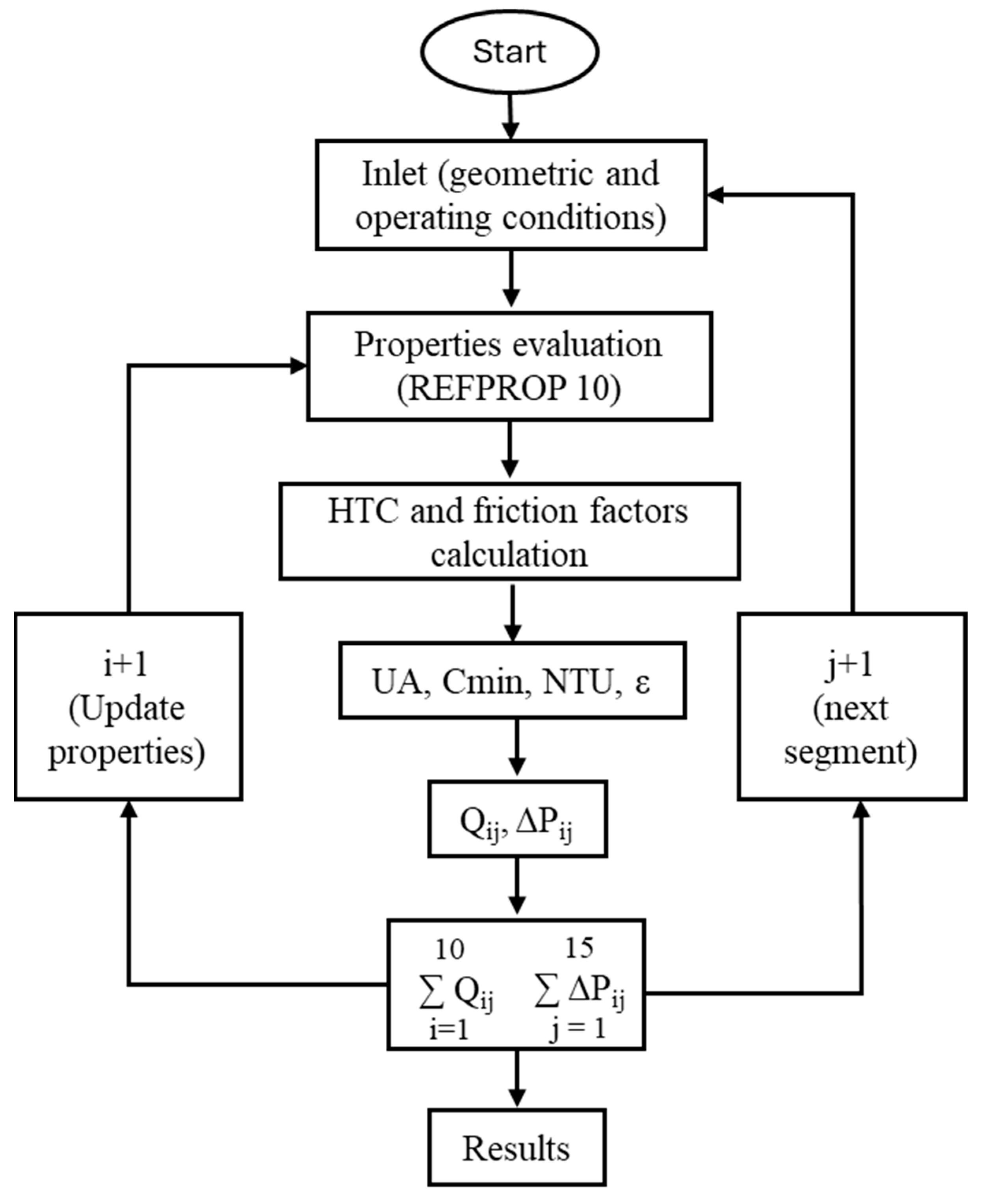
Accurate prediction of the thermohydraulic performance of MCGCs for EV applications is essential for their design and optimization. Conventional methods such as empirical correlations and numerical simulations have been extensively used in the field of heat transfer for evaluating the performance of MCGCs. These well-established techniques rely on physical principles and consider specific system details, including geometry, materials, and working fluid properties. Empirical correlations are basically derived from experimental data and are often tailored to specific geometries and flow regimes. Although these correlations offer a quick and straightforward solution, their accuracy may be limited, especially when applied to novel designs or nonstandard operating conditions. In contrast, numerical simulations offer a more comprehensive evaluation of the MCGC performance. Computational fluid dynamics (CFD) techniques such as finite element and finite volume methods are utilized to numerically solve the governing equations of fluid flow and heat transfer. These methods consider the intricate geometry of microchannels, the properties and behavior of the working fluid. By discretizing the domain and iteratively solving the equations, CFD simulations can provide insights into the thermohydraulic performance of MCGCs under various operating conditions. Both empirical correlations and numerical simulations have their advantages and limitations. Empirical correlations are relatively simple and can provide quick estimates; however, they may lack accuracy for complex designs or under unconventional operating conditions. Conversely, numerical simulations offer a more detailed understanding of the underlying physical processes but require significant computational resources and expertise. Both approaches have been widely used considering the specific details of the system being modeled. In addition, emerging techniques such as neural networks offer promising options for more accurate, cost effective, and quick estimation of MCGC performance [
6,
7,
8]. Neural networks can learn complex relationships between input parameters (e.g., geometrical and operational variables) and the corresponding thermohydraulic performance. By training the neural network with a diverse dataset generated from experimental or simulation data, MCGC performance can be accurately predicted under various operating conditions. ML algorithms are faster than numerical simulations, allowing for more rapid optimization of air conditioning system design. In addition, they are more flexible than numerical simulations, enabling performance prediction under a wider range of operating conditions and cooler designs. ML techniques have been extensively studied in heat transfer and fluid mechanics [
9,
10].
Saeed et al. [
11] performed 3D-Reynolds-averaged Navier–Stokes simulations to calculate the heat sink performances with various fin configurations. Subsequently, this data was employed to train six ML regression techniques to identify the most accurate method for predicting heat transfer coefficients and ΔP values. The selected ML model was combined with a multi-objective genetic algorithm to determine the ideal heat sink geometry. The multilayer perceptron method, adapted into a deep neural network model, effectively predicted the heat transfer coefficients and ΔP using the available data. The performance of the optimized channel geometry increased 2.1 times compared to that of the best existing channel configuration, with a 14% higher heat transfer coefficient and five times lower ΔP. Arman et al. employed a committee neural network (CNN) to estimate the ΔP in microchannels under varying conditions and demonstrated that incorporating multiple techniques into the CNN increased the accuracy of the results, suggesting its strong predictive potential across diverse fields [
12]. Kim et al. developed general ML models using power law regression and a database comprising 906 data points from 15 different sources. The ML models were found to have mean absolute errors of 7.5–10.9%, an approximately fivefold improvement in prediction accuracy compared with existing regression correlations [
13]. Yu et al. performed numerical simulations of the flow and heat transfer process in an elliptical pin-fin microchannel heat sink, and ANNs were used to predict the average temperature, temperature nonuniformity, and ΔP of the microchannel [
14]. Sikirica et al. introduced a framework using CFD, ML-based surrogate modeling, and multi-objective optimization to optimize microchannel heat sink designs. The optimized designs showed enhanced performance while reducing the computational time compared with traditional methods. The designs generated achieved temperatures more than 10% lower than that of a typical microchannel design under the same pressure limits. When limited by temperature, ΔP decreased by more than 25% [
15].
Recent advancements underscore the growing role of machine learning (ML) and deep learning (DL) in optimizing thermal system performance, particularly in complex geometries and multiphase flow conditions. For example, Zohora et al. [
16] applied multi-layer perceptron and XGBoost models to CFD data from pin-fin microchannel heat sinks, achieving over 95% accuracy in thermal and fluid flow predictions. Efatinasab et al. [
17] developed ANN and CNN models trained on a large experimental dataset to predict heat transfer and ΔP in micro-finned tube heat exchangers, achieving mean absolute errors under 4.5% and leveraging SHAP analysis for interpretability. Similar trends are evident in vortex generator optimization [
18], multimodal data fusion for boiling heat sinks [
19], and hybrid physics-informed frameworks for pool boiling on structured surfaces [
20]. Other works demonstrate the effectiveness of LSTM and Transformer-based models in capturing complex flow dynamics in plate heat exchangers [
21,
22], while XGBoost and SGBoost models have proven to be reliable surrogates for CFD in nanofluid systems [
23,
24]. Collectively, these studies highlight the current shift toward data-driven modeling strategies in thermal engineering, emphasizing high accuracy, physical interpretability, and substantial reductions in computational cost.
To meet the growing demand for compact, energy-efficient, and eco-friendly thermal systems in electric vehicles, transcritical CO2 microchannel gas coolers (MCGCs) have emerged as a promising solution due to their high heat transfer efficiency and low environmental impact. However, their design and operation involve significant challenges, such as complex two-phase flow, maldistribution, high-pressure conditions, and performance sensitivity to varying parameters. While experimental and CFD-based approaches have been used to investigate these systems, they often have high computational and resource costs, particularly when analyzing a wide range of conditions. In this context, machine learning (ML) offers a powerful and efficient alternative for predicting thermohydraulic performance by capturing nonlinear interactions among design and operating variables. This study aims to develop and validate ML-based models to provide fast and accurate predictions for MCGCs, supporting advanced design and optimization efforts.
In this work, we aim to investigate and compare the ability of ML algorithms in predicting the thermohydraulic performance of an MCGC for mobile air conditioning applications. Utilizing over 11,000 data points from an experimentally validated numerical model, we developed and optimized predictive models using five ML techniques: XGB, RF, SVR, KNNs, and ANNs. By carefully tuning hyperparameters and evaluating performance metrics such as coefficient of determination (R2) and mean squared error (MSE), our study provides insights into the unique abilities of each model, offering enhancement of the energy efficiency and design optimization of complex thermal systems in automotive applications.
3. Predictive Modeling of MCGC Using Machine Learning Approach
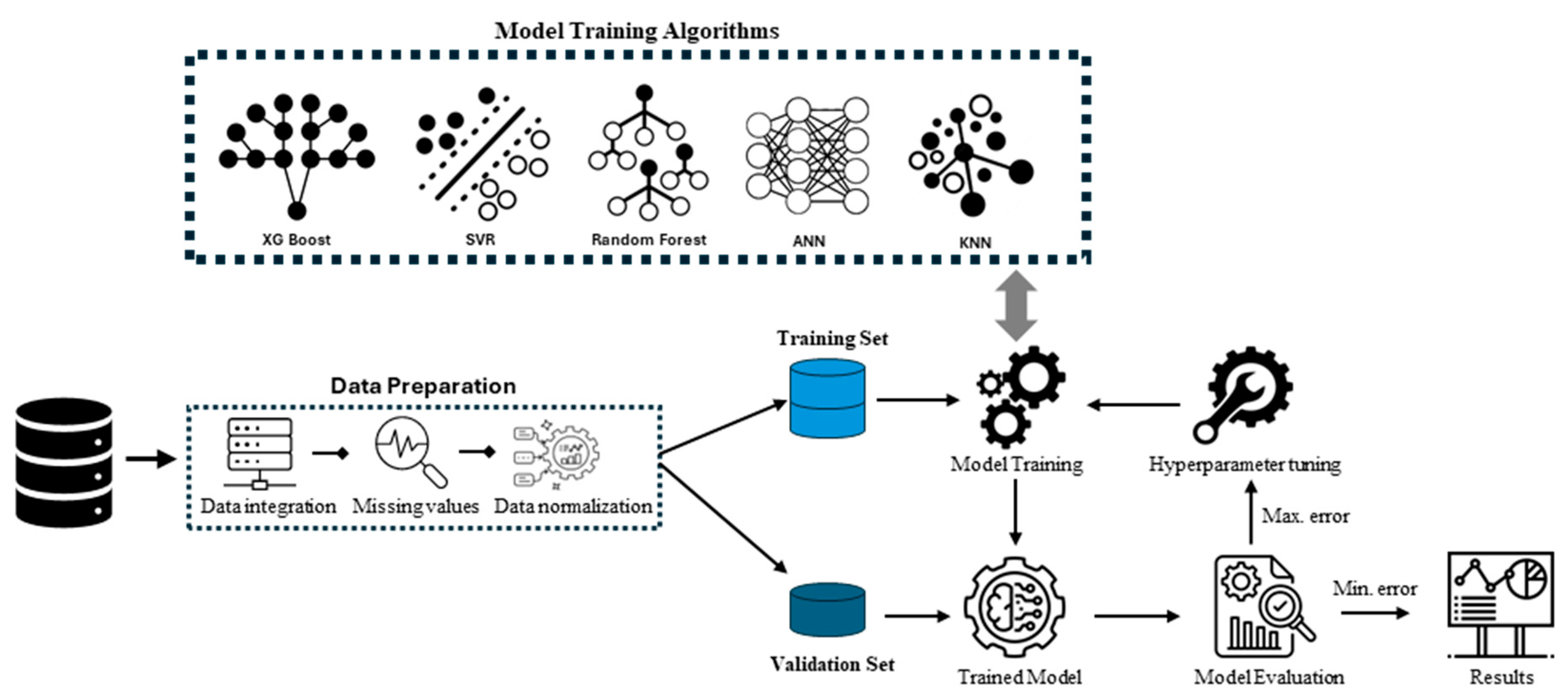
The methodology for predicting MCGC performance in mobile air conditioning systems (MACSs) is built upon a robust machine learning (ML) framework that incorporates five advanced algorithms: XGB, RF, SVR, KNN, and ANNs. Each algorithm was selected to represent a diverse range of modeling approaches, ensuring a comprehensive evaluation of their individual capabilities, from XGB’s robustness in handling tabular data to RF’s resilience against overfitting, SVR’s efficiency in capturing non-linear patterns, KNN’s interpretability for local relationships, and ANN’s capacity to learn intricate, non-linear interactions. By comparing their performance on the same dataset, the framework facilitates a comparative analysis of their performance, highlighting both their general-purpose utility and scenario-specific strengths. All algorithms were implemented using the scikit-learn library, with configurations tailored to optimize predictive accuracy while minimizing the risk of overfitting. This systematic and well-rounded approach provides valuable insights into the strengths and limitations of each algorithm, enabling informed decision-making for performance prediction in MACSs.
3.1. Problem Formulation
The task of performance prediction is framed as a supervised learning problem. Given a dataset containing input features
, where
n is the number of features, representing geometric and operational parameters, and output variables
, where m is the number of output variables, representing system performance metrics, the objective is to learn the functional relationship:
where
is the true mapping function and
is the error. Each algorithm separately models this relationship, predicting the outputs
. To evaluate model performance, two metrics were used: mean squared error (MSE) and the coefficient of determination (R
2). The MSE is defined as follows:
which quantifies the average squared difference between predicted
and true
values. The R
2 metric is defined as follows:
measures the proportion of variance in the dependent variable that is predictable from the independent variables.
The overall workflow of the system is depicted in
Figure 4, providing a clear representation of the sequential processes involved. Each component of the workflow is meticulously detailed in the subsequent sections, offering an in-depth explanation of their roles and functionality within the system.
3.2. Data Preparation
The dataset used for machine learning model development was generated from a validated numerical model of the MCGC [
27,
28]. By systematically varying key geometric and operational parameters such as number of passes (3–5), number of tubes (18–60), number of circular ports (9–21), ambient temperature (42–56°C), inlet air flow rate (0.45–0.70 kg/s), and refrigerant flow rate (0.018–0.057 kg/s), a total of approximately 13,000 datasets were generated. Each data point includes twenty-three input parameters and four output performance indicators. While the numerical model exhibits some errors relative to experimental data, our ML framework will be trained and tested exclusively on those same simulated outputs, so this bias will not affect the reported ML accuracy.
The dataset was thoroughly examined for missing, constant, and duplicate values, followed by necessary preprocessing steps to ensure its integrity and readiness for analysis. A rigorous approach was also applied for outlier removal to maintain the quality of the regression modeling. To enhance predictive accuracy and model efficiency, a systematic feature selection process was carried out on the preprocessed dataset. Statistical techniques and correlation analysis were used to identify the most influential variables affecting the target outputs, thereby reducing the original 27 features to an optimized set of 13 (nine input features and four output features). Features with constant values such as heat exchanger volume, tube pitches, fin pitch, tube thickness, and fin height were removed due to their lack of variance. Redundant features were excluded based on high correlation and engineering relevance. For example, among airflow-related parameters (velocity, mass flow rate, and volume rate), only the air mass flow rate was retained. Similarly, the number of tubes and number of ports were chosen over the more dependent geometric dimensions like height and width. A single categorical feature “passes” was used to represent the variation in refrigerant flow configurations. This refined feature set not only reduces model complexity and the risk of overfitting but also ensures better interpretability and relevance to the thermal and hydraulic behavior of CO2 gas coolers.
The input features include air flow rate (ṁ
ca), air inlet temperature (T
cai), refrigerant flow rate (ṁ
r), refrigerant inlet pressure (P
cri), refrigerant inlet temperature (T
cri), heat exchanger length, number of tubes, ports, and passes. Output variables are Q, ∆P, and air and refrigerant outlet temperatures (T
ao and T
ro). Ranges of geometric and operating conditions for machine learning models are given in
Table 3.
3.3. Train Test Split Technique
In ML, evaluating a model’s performance on unseen data is crucial for the assessment of its generalizability. To achieve this, the dataset is commonly divided into two subsets: a training set and a testing set. The training set is used to train the model, enabling it to learn the underlying patterns and relationships between the input features and output values. On the other hand, the testing set is employed to assess the model’s performance on new, unseen data, which helps determine how effectively the model can generalize its predictions to novel data points. In this study, the testing set size was defined as 0.2, indicating that 20% of the dataset was dedicated to testing, while the remaining 80% was allocated for the training set. Moreover, the random state parameter was set to 1, ensuring that the data split was reproducible across multiple runs. By setting this parameter, we obtained consistent results when evaluating the models. Consequently, the resulting training set, represented as Xtrain (input features) and ytrain (output values), was employed to train various models, and the testing set, denoted as Xtest (input features) and ytest (output values), was used to evaluate the performances of these models. Using this systematic approach, we effectively determined the capabilities and limitations of the different models under consideration.
3.4. Model Training
As described earlier, five different machine learning algorithms, i.e., XGB, RF, SVR, KNN, and ANNs, were independently used to train multiple models. Each algorithm was optimized using hyperparameter tuning to ensure accurate predictions and robust performance across the dataset. To prevent overfitting, early stopping techniques were employed during model training.
3.4.1. Algorithms for MCGC Performance Predictions
These algorithms were implemented using Python 3.11, and utilized a suite of powerful open-source libraries. For seamless data handling and preprocessing, pandas enabled efficient loading and manipulation of tabular datasets, while NumPy facilitated complex mathematical computations. To visualize insights and trends, matplotlib provided dynamic and intuitive plotting capabilities. Key machine learning operations, including data transformation, model implementation, and evaluation, were powered by scikit-learn. Specifically, sklearn.linear_model supported the implementation of various regression models, sklearn.preprocessing ensured the data was appropriately transformed, sklearn.model_selection streamlined data splitting and cross-validation, and sklearn.metrics allowed for comprehensive performance evaluation using diverse metrics. Together, these tools not only enabled precise coding of the models but also ensured their performance could be rigorously assessed. Each algorithm’s underlying principles were carefully considered to match the dataset’s complexity and diversity, creating a framework that combines analytical rigor with computational efficiency.
The Extreme Gradient Boosting Algorithm
XGB, introduced by Chen [
29], is a powerful ML algorithm that belongs to the class of ensemble methods. It builds an ensemble of weak learners (decision trees) in a sequential, additive manner while minimizing a given loss function to form a strong predictive model. XGB employs regularization techniques to control model complexity and reduce overfitting. The objective function of XGB can be expressed as follows:
where
is the model parameters,
is the loss function,
is the true label of the ith observation,
is the predicted label of the
ith observation at the (t − 1)th iteration,
is the
tth weak learner (i.e., decision tree) that maps the features (
xi) to a predicted label, and
is a regularization term that penalizes complex models. The objective function comprises two parts: the loss function and the regularization term. The loss function measures the difference between the predicted and true labels, whereas the regularization term penalizes complex models to avoid overfitting.
Figure 5 shows the schematic of the XGB model.
Random Forest Algorithm
RF is an ensemble learning algorithm developed by Breiman and Leo [
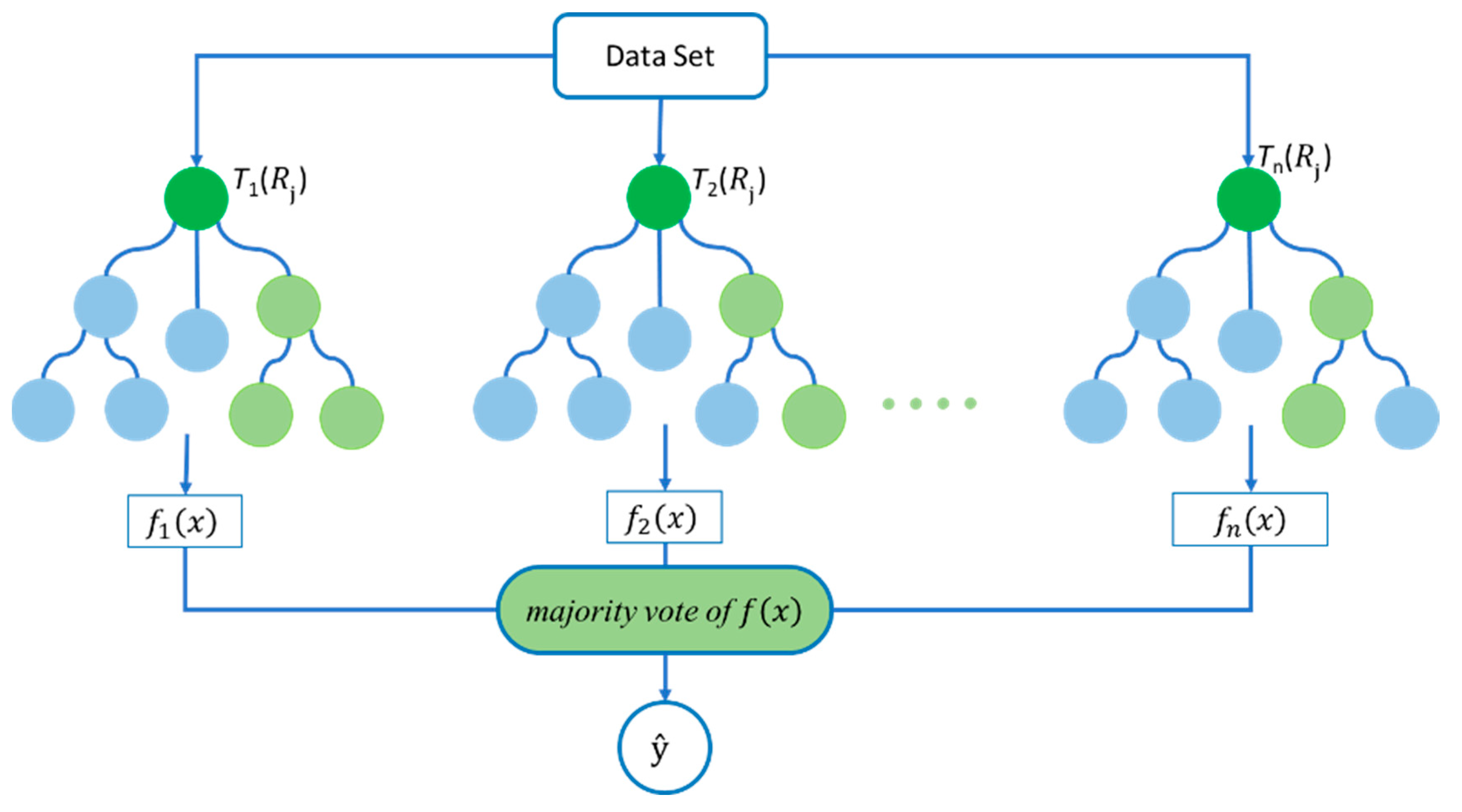
30]. It combines multiple decision trees to improve the accuracy and robustness of the model. The mathematical equation for the RF model is expressed in Equation (10) as follows:
where
is the predicted value for a new observation with the feature vector
x. The decision tree comprises a set of regions
that divide the feature space into mutually exclusive and exhaustive regions. Each region
is associated with the predicted value
. The equation
I(
x∈
) is an indicator function that takes the value 1 if the new observation
x belongs to region
and takes the value 0 otherwise. Therefore, Σ(
* I(
x∈
)) computes the predicted value by summing the predicted values
of all regions to which the new observation x belongs:
In Equation (11),
is the predicted value for the new observation with the feature vector
x. It comprises
n decision trees trained on the randomly selected subsets of the training data and the randomly selected subsets of the features. Each decision tree produces the predicted value
for the new observation
x. The function mode returns the most common value among its arguments, which are the predicted values of all the decision trees. Therefore, the equation
computes the predicted value by taking the majority vote of the predicted values of all decision trees in the RF. The schematic of the RF model is shown in
Figure 6.
Support Vector Regression Algorithm
SVR is an ML algorithm developed by Vapnik and fellows [
31] for regression tasks. It is a variant of support vector machine (SVM) and is particularly useful when dealing with nonlinear and complex data using different kernel functions. SVR aims to find the best-fitting hyperplane that maximizes the margin while minimizing the prediction error. SVR can be expressed as follows:
where
y is the target variable, b is the bias term, and
are the Lagrange multipliers or support vector weights associated with each data point.
K(
) is the kernel function that calculates the distance between the input data points
and
in a higher-dimensional feature space.
k-Nearest Neighbors Algorithm
In ML, a KNN is a nonparametric algorithm that predicts the value of a target variable by considering the k-nearest training examples in the feature space. To determine the nearest neighbors, the KNN algorithm uses a distance metric to measure the distance between each pair of observations in the feature space. The most used distance metric is the Euclidean distance, which can be described by Equation (13):
where
is the
kth feature of observation
i, and
is the kth feature of observation
j.
Once the distance between each pair of observations is calculated, the algorithm selects the KNNs for the new observation. The value of
k is a hyperparameter set before training the algorithm. Then, the KNN algorithm assigns the label of the new observation based on the majority class of its KNNs, as described by Equation (14):
where
is the predicted label for the new observation,
is the label of the
ith nearest neighbor, and
I(
yi =
y) is an indicator function that equals 1 if
=
y and 0 otherwise. The function argmax returns the value of the argument that maximizes the function inside the parentheses. In other words, argmax returns the label
y that has the highest frequency among the KNNs.
Artificial Neural Networks Model
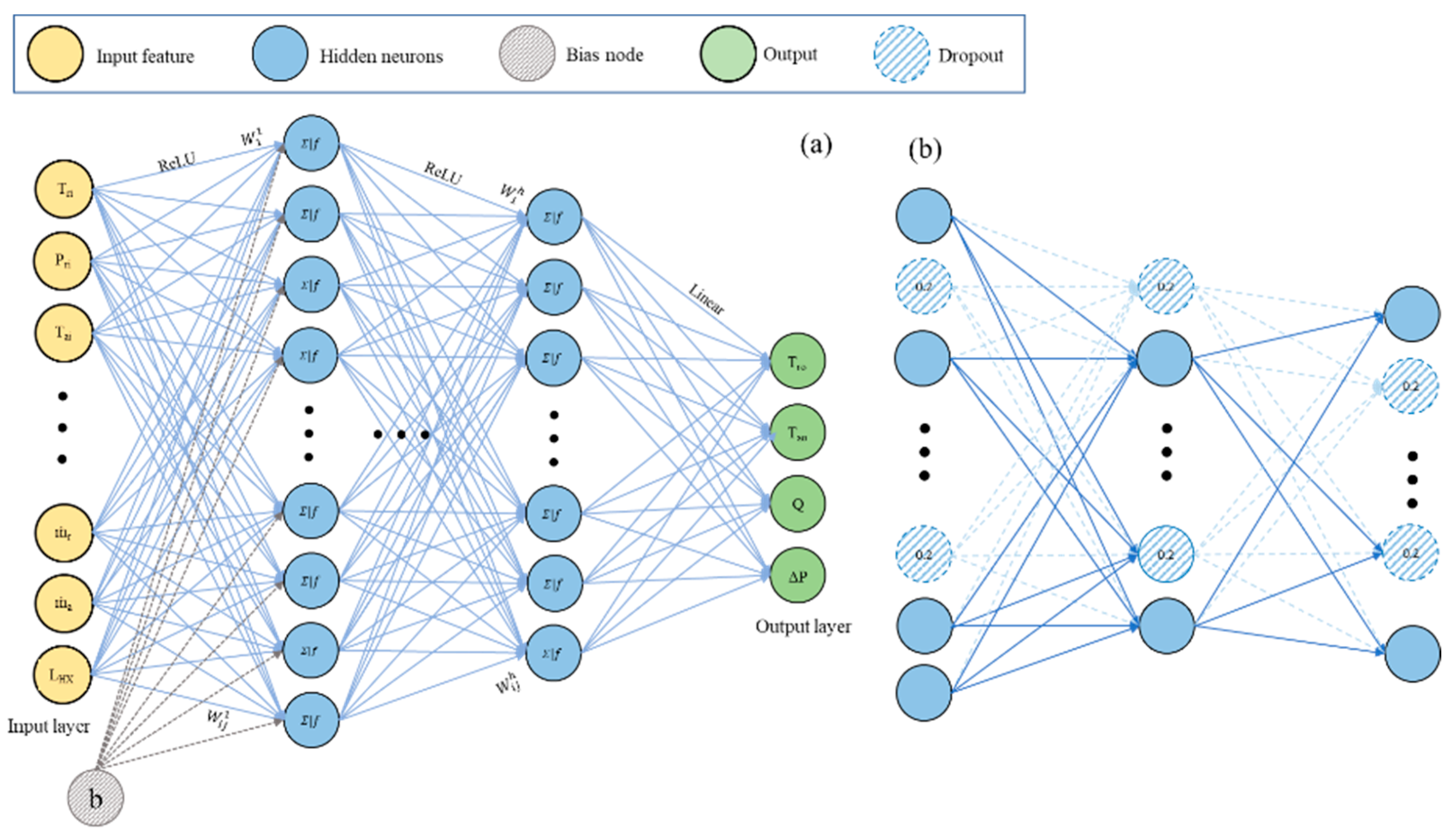
ANNs are computational models inspired by biological neural networks and are used in various ML applications. They comprise interconnected layers of neurons, including the input, hidden, and output layers as shown in
Figure 7. ANNs learn through backpropagation, adjusting their weights to minimize the error between the predicted and actual outputs. Activation functions introduce nonlinearity, enabling the network to learn complex relationships, as described by Equation (15):
where
represents the preactivation value of neuron
i in the hidden layer
h,
denotes the weight connecting neuron
j in layer (
h − 1) to neuron
i in layer
h,
represents the activation value of neuron
j in layer (
h − 1), and
represents the bias term associated with neuron
i in layer
h.
is the number of neurons in layer (
h − 1).
The topology of the ANN employed in predicting the performance of an MCGC comprised an input layer, three hidden layers, and an output layer. In total, 9 features were considered, with model outputs including Tao, Tro, Q, and ∆P.
To prevent overfitting and enhance generalization, the dropout technique is utilized in neural networks. This technique selectively deactivates neurons in hidden layers during training, thus improving the network’s ability to generalize unseen data. Through dropout regularization, the architecture of the neural network is adjusted, contributing to more robust model performance.
3.5. Hyperparameter Tuning
The predictive capability of an ML model heavily relies on fine-tuning its hyperparameters. Hyperparameters are configuration settings that are not directly learned from the data but influence the learning process. Optimizing these hyperparameters is crucial to achieve the best model performance. In ML, various methods are commonly employed to fine-tune a model’s hyperparameters. The manual search involves manually tweaking the hyperparameters based on prior knowledge and intuition. The grid search systematically explores a predefined grid of hyperparameter combinations and evaluates the model’s performance for each configuration. Moreover, the random search employs a randomized search strategy by sampling hyperparameters from predefined distributions. In this study, the RandomizedSearchCV method is used for parameter tuning. RandomizedSearchCV combines the benefits of random search and cross-validation. It randomly samples hyperparameters from the defined distributions and evaluates the model’s performance using cross-validation techniques. This approach allows for a more efficient exploration of the hyperparameter space, enabling the identification of promising combinations that yield improved model performance. Once the hyperparameters are fine-tuned using RandomizedSearchCV, the model is deemed ready for training, testing, and prediction. With the optimized hyperparameters, the model can be trained on the training data, allowing it to learn the underlying patterns and relationships. Subsequently, the model’s performance is assessed on the testing set to evaluate its ability to make accurate predictions on unseen data. Finally, with the trained and evaluated model, predictions can be made on new, unseen data to facilitate decision-making and inference tasks.
4. Results and Discussion
4.1. Feature Importance
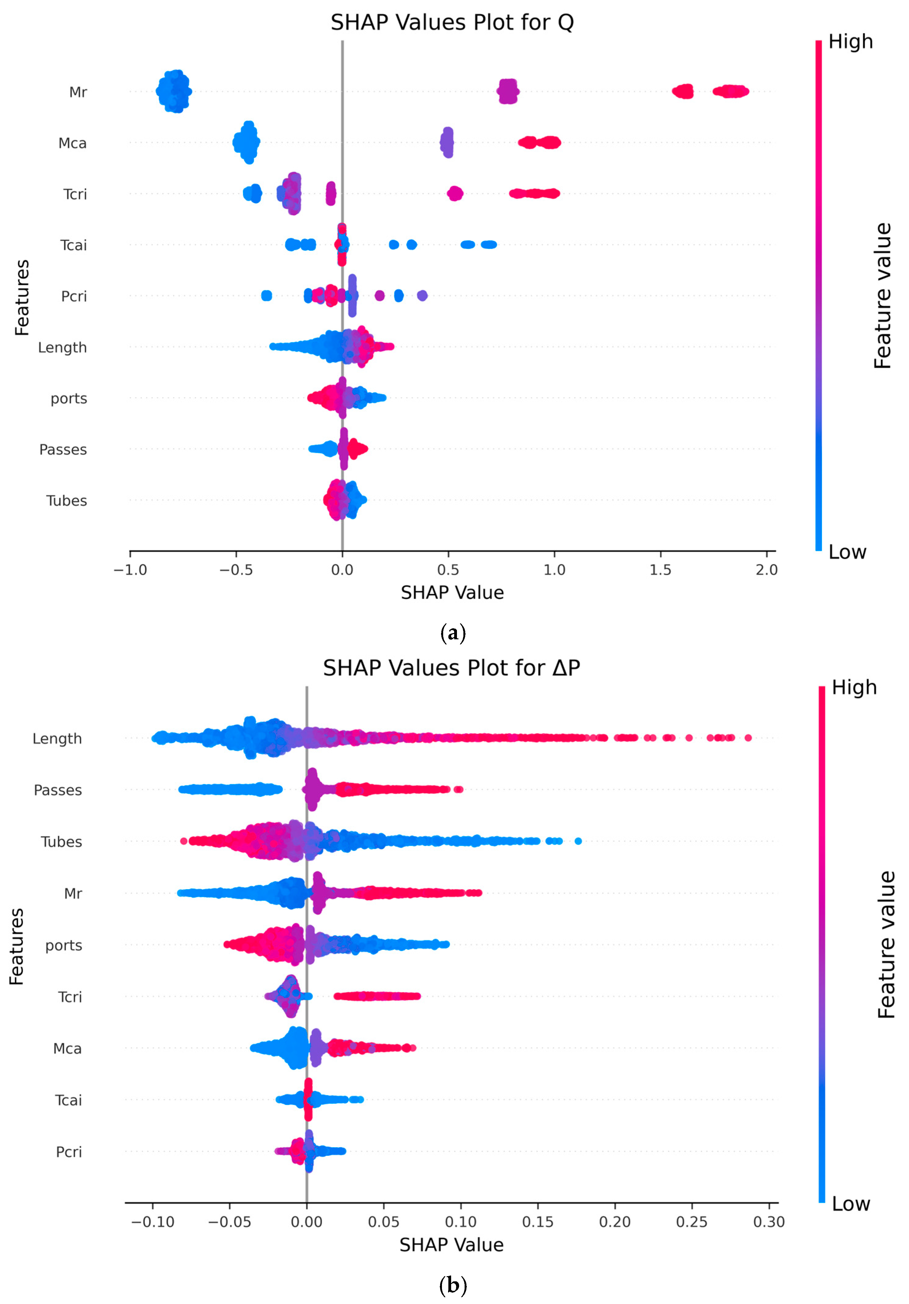
The SHAP analysis provides a detailed interpretation of feature contributions to the machine learning model’s predictions for both Q and ΔP in the gas cooler system. As shown in
Figure 8a, for the output variable Q, the ṁ
r emerges as the most influential parameter, as indicated by consistently high SHAP values. This reflects the direct thermodynamic relationship between increased refrigerant flow and higher heat capacity. The ṁ
ca also contributes positively to Q, although with slightly less variability than ṁ
r. A higher air flow rate enhances the convective heat transfer on the air side, thereby increasing overall heat transfer. The T
cri shows a positive impact on Q at higher values, indicating that warmer T
cri improves the energy transfer potential. In contrast, the T
cai displays a negative relationship with Q, meaning lower T
cai values result in larger temperature differentials between air and refrigerant, enhancing heat transfer and increasing Q. The P
cri has a minimal effect, as evidenced by SHAP values clustered near zero, suggesting a negligible marginal contribution under the modeled conditions.
Regarding the geometrical parameters, tube length demonstrates a significant positive influence on Q. A longer tube provides an extended heat transfer surface area and contact time, enhancing thermal exchange. The number of passes also positively affects Q, as it increases the effective refrigerant path length. However, the number of tubes and ports shows a negative impact on Q. This may be attributed to the division of flow among a higher number of channels, potentially reducing the velocity and convective heat transfer effectiveness in individual tubes or ports. Overall, the operating conditions exert a more dominant influence on Q than the geometrical features.
In contrast, the SHAP analysis for ΔP, as illustrated in
Figure 8b, reveals a shift in the dominant contributing features. Tube length again shows the highest impact, with longer lengths correlating with increased ΔP due to higher frictional losses over a longer path. Similarly, an increased number of passes leads to higher ΔP, as the flow is redirected more frequently, increasing turbulence and head loss. The number of tubes has a negative contribution; more tubes reduce ΔP by allowing a greater number of parallel flow paths, thereby reducing the velocity and associated frictional losses per tube. The ṁ
r has a strong positive impact on ΔP, as higher flow rates increase velocity and, consequently, the pressure loss due to friction. The number of ports shows a negative influence, possibly due to more distribution and reduced local velocities. Notably, the SHAP values for operating conditions such as T
cri, ṁ
ca, T
cai, and P
cri are relatively low, indicating minimal effect on ΔP compared to geometrical parameters. Overall geometrical features dominate the contributions to ΔP while operating parameters have less impact.
These findings highlight the importance of distinguishing the roles of thermodynamic and geometric parameters in influencing different aspects of gas cooler performance. The SHAP analysis not only quantifies each feature’s impact but also aligns with engineering principles, offering interpretable and physically consistent insights into the model’s decision-making process.
4.2. Gas Cooler Capacity Predictions
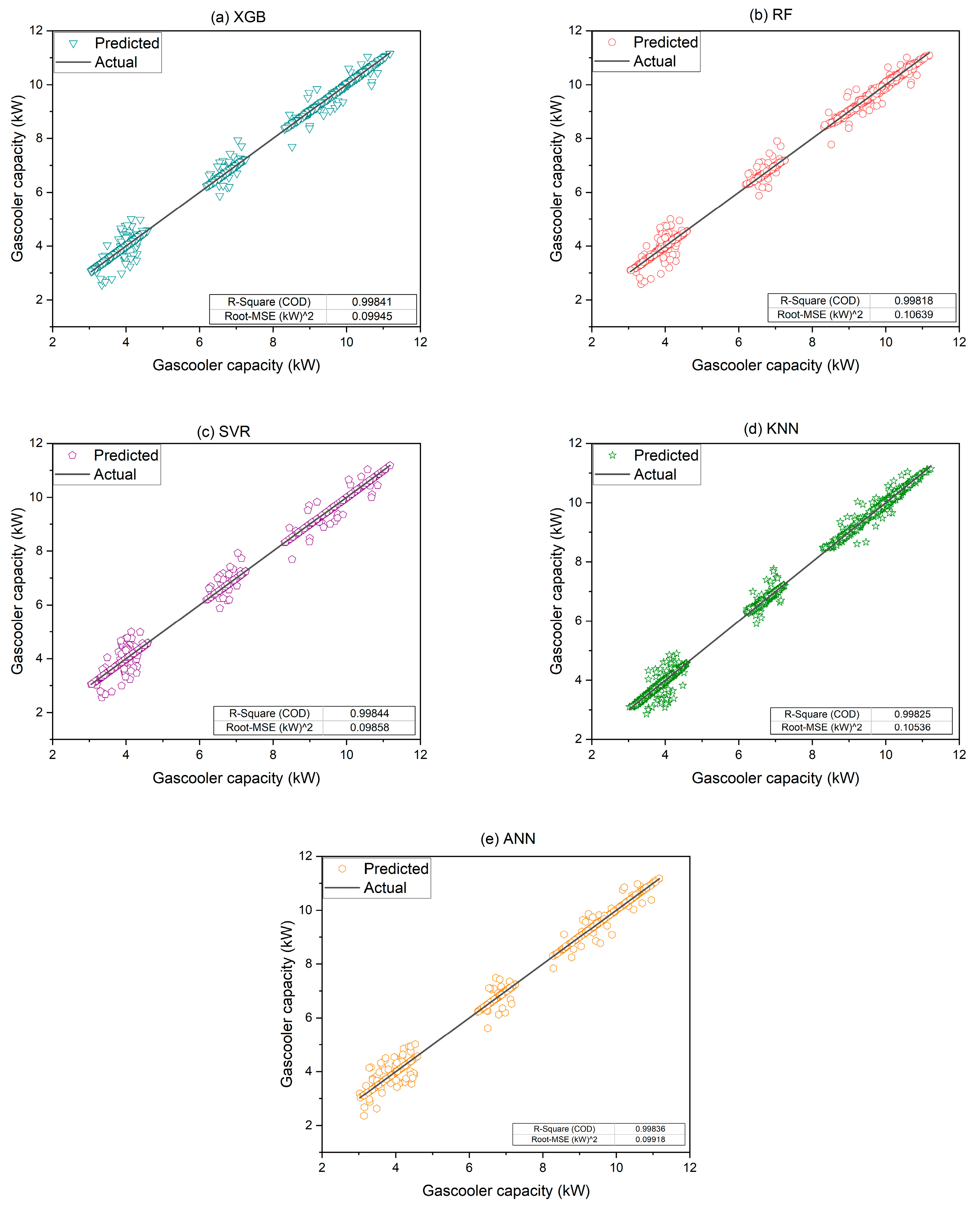
In
Figure 9a–e, the predicted Q of an MCGC is visually represented using advanced ML models such as (a) XGB, (b) RF, (c) SVR, (d) KNNs, and (e) ANNs. Two key metrics, the coefficient of determination (R
2) and the mean squared error (MSE), were used to evaluate the performance and accuracy of each model. The R
2 values, which reflect the proportions of predictable variance, showcase excellent predictive performance across all models, with XGB at 0.99841, RF at 0.99818, SVR at 0.99844, KNNs at 0.99825, and ANNs at 0.99836. Simultaneously, the MSE values, which indicate the average squared differences between the predicted and actual values, exhibit noteworthy accuracy, with XGB at 0.09945, RF at 0.10639, SVR at 0.09858, KNNs at 0.10536, and ANNs at 0.09918.
Possible reasons for obtaining these results are attributed to the inherent strengths of each algorithm. XGB, known for its ensemble learning and boosting techniques, reveals high accuracy and efficiency in capturing complex patterns in the data. RF utilizes multiple decision trees, provides robustness in handling diverse features and reducing overfitting. SVR, which is based on the identification of optimal hyperplanes, excels in handling nonlinear relationships in the data. KNNs rely on proximity and are effective in capturing local patterns and dependencies. Lastly, ANNs, inspired by human brain functioning, showcase significant performance in capturing intricate relationships in large datasets. The combined use of these models allows for a comprehensive evaluation, providing valuable insights into Q predictions and aiding in the selection of the most suitable model for practical applications.
4.3. Gas Cooler Pressure Drop Predictions
The graphical results shown in
Figure 10a–e represent ΔP predictions using XGB, RF, SVR, KNNs, and ANNs. As with the capacity prediction, R
2 and MSE were used to assess model reliability, showing consistently high accuracy across all approaches. Notably, XGB stands out with an exceptional R
2 value of 0.99398, highlighting its robust capability in predicting ΔP. SVR and ANNs also exhibit significant R
2 values of 0.99166 and 0.98954, respectively, emphasizing their accuracy. RF maintains a notable R
2 value of 0.96809, whereas the KNN model, with its focus on proximity-based predictions, displays a somewhat lower R
2 value of 0.86713. This is primarily due to the local nature of KNN, which performs well in dense regions but lacks a global modeling structure, making it less suitable for capturing complex ΔP patterns. In contrast, ANN excels by modeling intricate non-linear dependencies, while XGB and SVR effectively manage high variance through boosting and margin optimization, respectively.
At the same time, the MSE values, which offer insights into the average squared differences between the predicted and actual values, confirm the accuracy of the models. XGB demonstrates exceptional precision with a low MSE of 0.12172, indicating minimal discrepancies in its ΔP predictions. SVR and ANN exhibit reliability with MSE values of 0.14033 and 0.13358, respectively. However, RF, despite its robust R2 value, presents a higher MSE of 0.25647, indicating some variability in prediction accuracy. The KNN model, which relies on local patterns, demonstrates a higher MSE of 0.45952, indicating potential challenges in capturing complex relationships within the data. The small variations in the performances of the models emphasize the importance of selecting suitable algorithms based on specific data characteristics and the complexities of the prediction task. Among all the models, XGB stands out as an effective predictor, producing impressive and reliable ΔP predictions. The RF model exhibits slight dispersion in its predictions. The SVR model presents more detailed behavior, providing dispersed predictions for lower ΔP while exhibiting enhanced accuracy for higher ΔP. This intriguing distinction shows the SVR model’s sensitivity to ΔP ranges and its potential applicability in scenarios with high ΔPs. In contrast, the KNN model shows considerable inconsistency, delivering highly dispersed predictions that deviate significantly from the acceptable range. Such divergence raises concerns about the suitability of the KNN model for ΔP analysis. On the other hand, the ANN model emerges as the best predictive model for ΔP prediction. The results highlight exceptional performance, surpassing the performance of other models. This superiority can be attributed to the ANN’s unique approach based on deep learning principles, enabling it to effectively capture complex patterns and dependencies in the ΔP data. XGB shows robust predictive capabilities, RF exhibits promise with slight fluctuation, and SVR reveals distinct behavior across ΔP ranges. While KNN’s highly dispersed predictions raise concerns about its reliability, the ANN model stands out as a dominant model due to its precision and accuracy in ΔP predictions, substantiating the power of deep learning techniques.
4.4. Refrigerant (CO2) Outlet Temperature Predictions
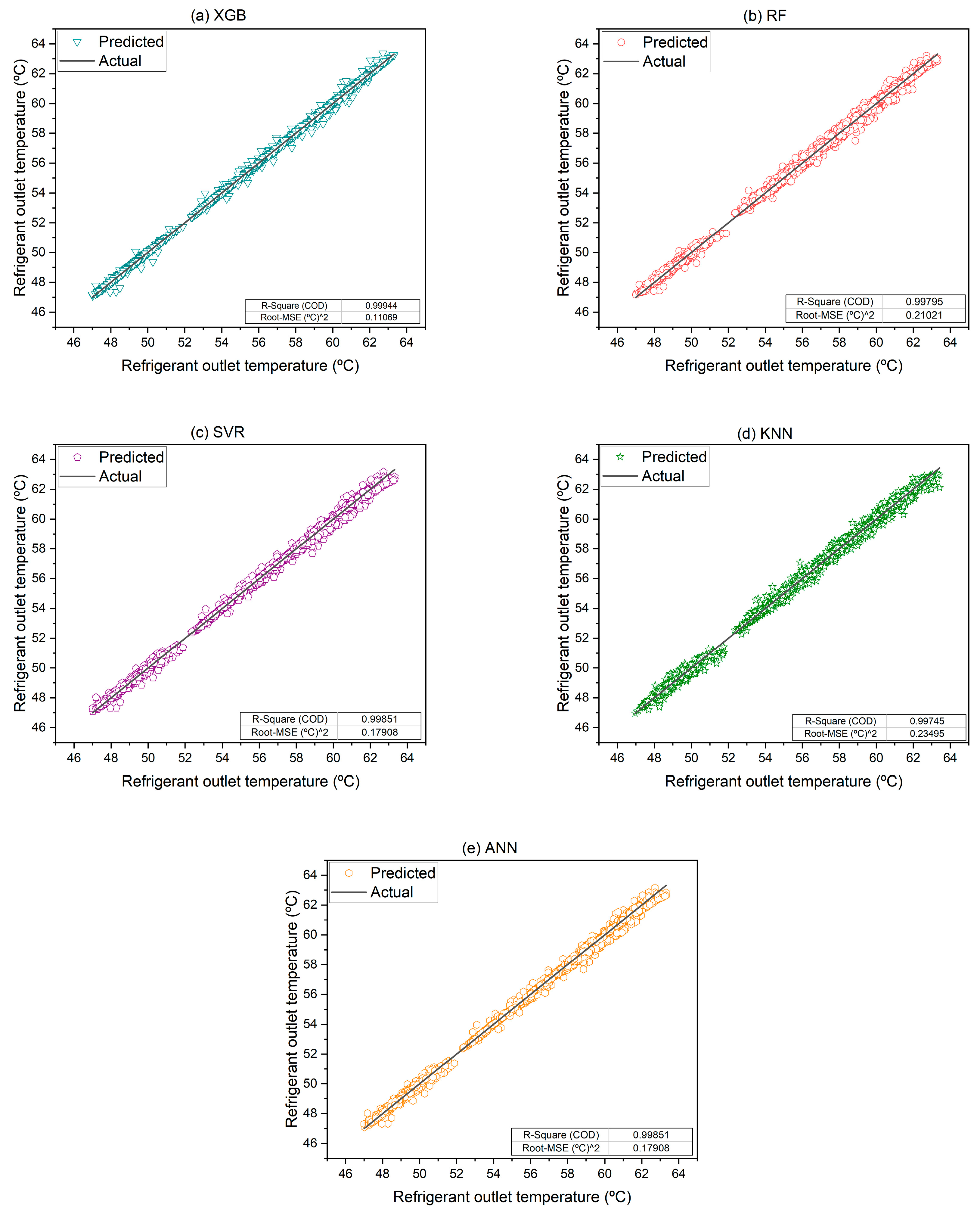
Figure 11 illustrates that all models reveal remarkable accuracy in their predictions of refrigerant (CO
2) outlet temperature. Among the models, the ANN demonstrates superior performance, providing the most accurate predictions of outlet temperature. This high level of precision can be attributed to its deep learning architecture, which effectively captures complex patterns and dependencies within the data, resulting in highly reliable outcomes. Furthermore, the SVR model notably avoids overfitting in this specific case. This indicates that SVR’s margin-based learning is well-tuned for smooth continuous outputs like temperature, though its performance may still be constrained in the presence of high-dimensional feature interactions, where ANN has a natural advantage.
4.5. Air Outlet Temperature Predictions
Our detailed assessment of predictive models for outlet air temperature forecasting revealed the notable potential of all models to achieve accurate predictions. Among them, the ANN model exhibits the highest precision and reliability in its predictions, as shown in
Figure 12. Its superior performance can be attributed to its utilization of sophisticated DL techniques, which enables it to discern intricate patterns and dependencies within the data. The XGB and SVR models closely follow the ANN model in proficiency, demonstrating commendable predictive capabilities. Their competitive performance attests to their capacity to capture meaningful insights from the data, although they fall short of the exceptional results achieved using the ANN model. Moreover, the RF and KNN models offer noteworthy outcomes, though RF may have oversmoothed predictions due to averaging across trees, and KNN’s instance-based learning is more sensitive to local variations, limiting its generalization across broader operating conditions.
4.6. Comparitive Analysis of Numerical Model and ANN
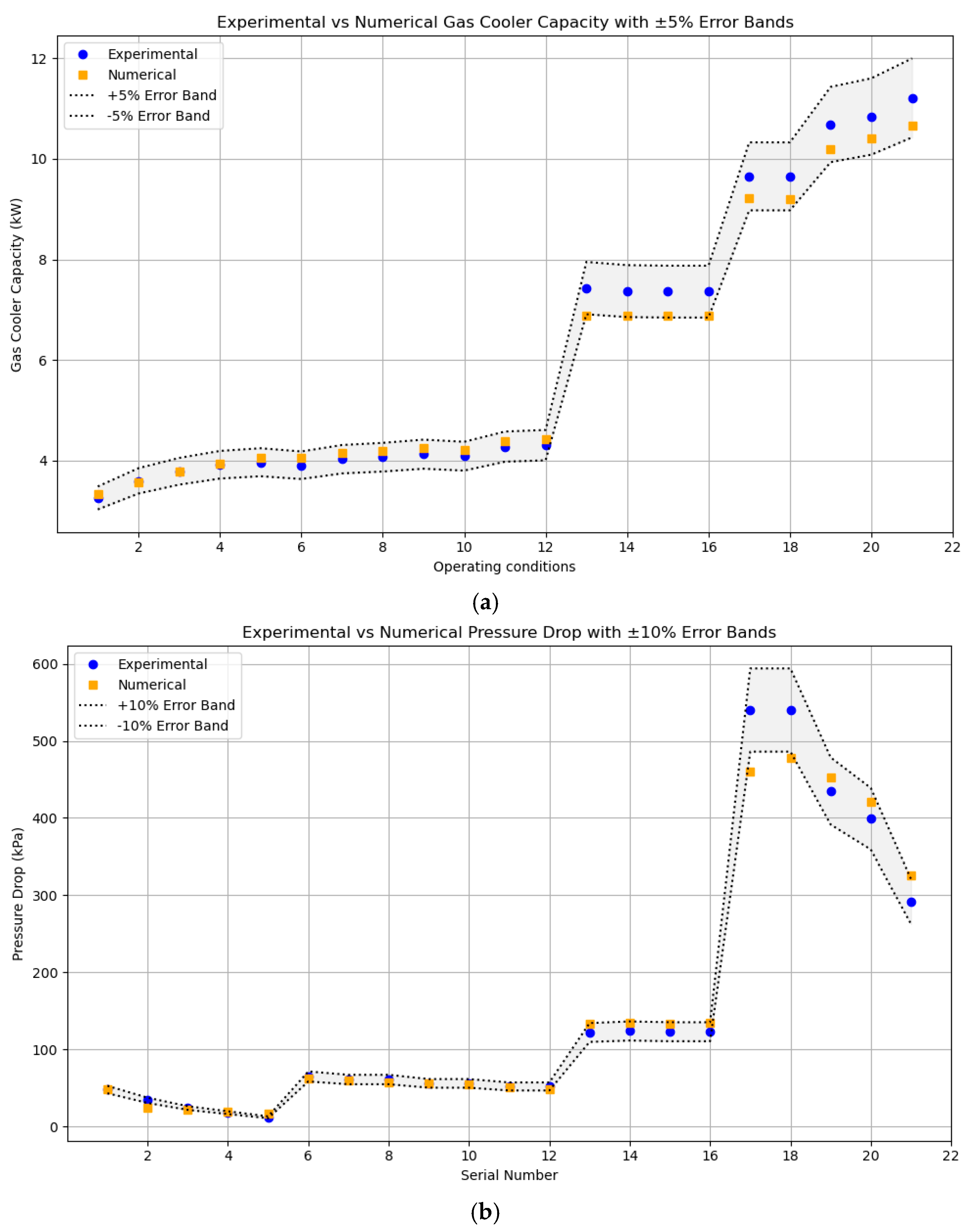
Figure 13a evaluates the percentage error in predicting Q by comparing experimental data with numerical simulation results, and numerical results with ANN predictions. The error between experimental and numerical results averages 3.63%, indicating that the numerical model effectively captures the thermal behavior of the gas cooler. This level of agreement suggests that the numerical model accurately incorporates the key thermophysical properties of the working fluid, heat transfer mechanisms, and flow distribution effects. On the other hand, the ANN model, trained on numerical data, demonstrates a slightly higher average error of 4.14%. This reflects the ANN’s capacity to generalize from training data and estimate thermal capacity under varying input conditions with reasonable accuracy. Despite the black-box nature of ANNs, their predictive reliability in this context highlights their suitability for quick performance estimation, especially when rapid analysis is needed in parametric studies or optimization routines.
Figure 13b analyzes the percentage error in predicting gas cooler ΔP, again comparing experimental data with numerical results, and numerical data with ANN predictions. ΔP prediction typically involves more sensitivity to geometric features, flow regime transitions, and localized effects such as entrance losses or maldistribution. The numerical model shows an average error of 6.05% when compared to experimental values, suggesting that while it captures the general trend, it may have limitations in modeling detailed flow resistance or minor losses. In contrast, the ANN model achieves a lower average error of 3.73% compared to the numerical results, indicating effective learning of the complex nonlinear mapping between inputs (e.g., geometric and operating conditions) and output (ΔP). Moreover, once the ANN model is trained, it can produce predictions in nanoseconds, offering a significant computational advantage over simulation-based methods, which are typically resource-intensive and time-consuming. This speed advantage makes ANN particularly attractive for real-time control, iterative design, and optimization applications.
5. Conclusions
This study employed various machine learning algorithms (XGB, RF, SVR, KNN, and ANN) to predict the thermohydraulic performance of a microchannel gas cooler (MCGC). The models were trained on high-fidelity data generated from a validated numerical model, and their hyperparameters were carefully optimized to ensure robust performance. SHAP plots were used to interpret models and identify the influence of key operational and geometric parameters.
Among the tested models, ANN consistently delivered the highest accuracy across all performance metrics, including Q, ΔP, and outlet temperatures. XGB and SVR also performed well in certain cases, while KNN showed limitations in consistency. SHAP-based interpretability helped uncover important trends, such as the significant effect of flow rates and air-side temperatures.
This work adds novelty by focusing specifically on transcritical CO2 MCGCs, a relatively less-explored application in ML-based thermal system modeling. The integration of explainable ML techniques (e.g., SHAP) further enhances its practical relevance, offering insights that can support the design and optimization of advanced cooling systems, particularly in automotive and energy applications.
From a comparative standpoint, the findings highlight the importance of aligning model choice with data characteristics. ANN’s deep learning framework excels at capturing intricate nonlinear relationships in complex thermofluidic data, while XGB’s ensemble boosting effectively reduces bias and variance. SVR demonstrates strength in handling smooth trends without overfitting, and RF provides stability through averaging, albeit sometimes at the cost of precision. KNN, despite being intuitive and easy to implement, is more sensitive to local noise and less suited for capturing global patterns. These distinctions offer guidance for model selection in future applications of ML in heat exchanger performance prediction.


