
Estimation of Wind Conditions in the Offshore Direction Using Multiple Numerical Models and In Situ Observations

 ,
,
Abstract

1. Introduction
- ➢
- Demonstrating the effectiveness of multi-point LiDAR observations for evaluating wind profiles across coastal and offshore zones.
- ➢
- Comparing model performance at hub-height levels under varying atmospheric stability.
- ➢
- Clarifying the influence of reference point selection on model accuracy.
- ➢
- Providing practical guidance for model application in nearshore wind resource assessments.
2. Data and Methods
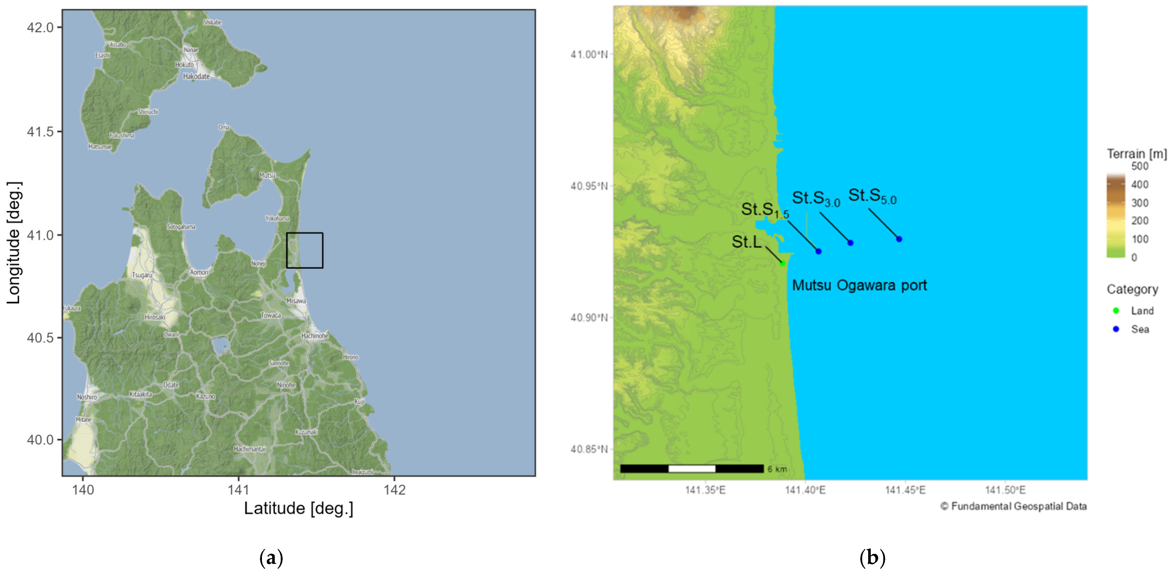
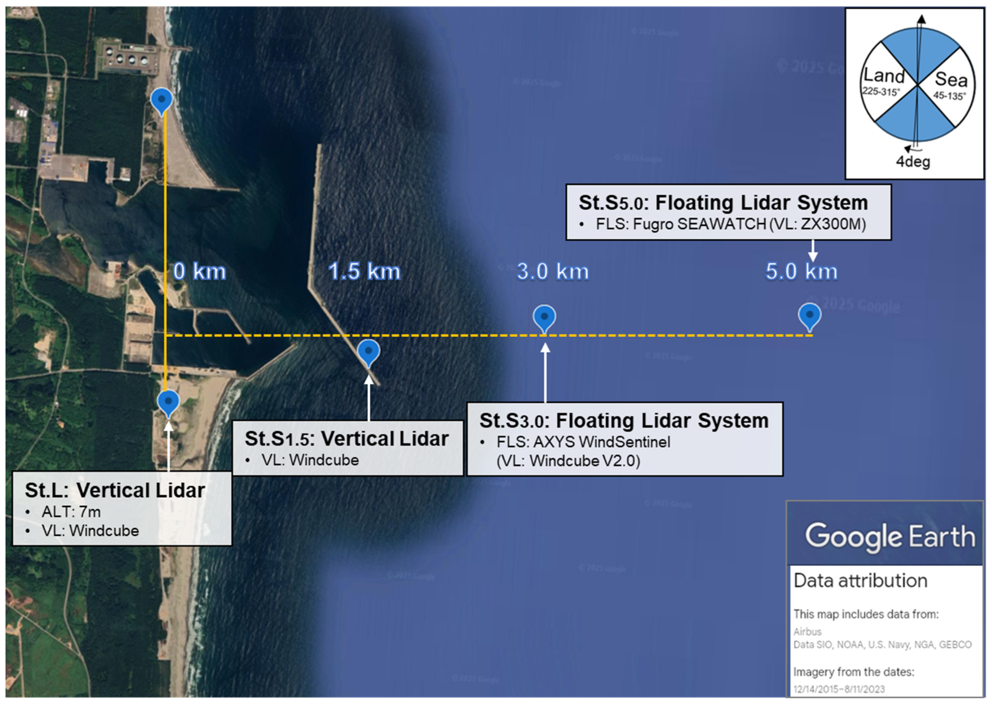
2.1. Experiment Overview
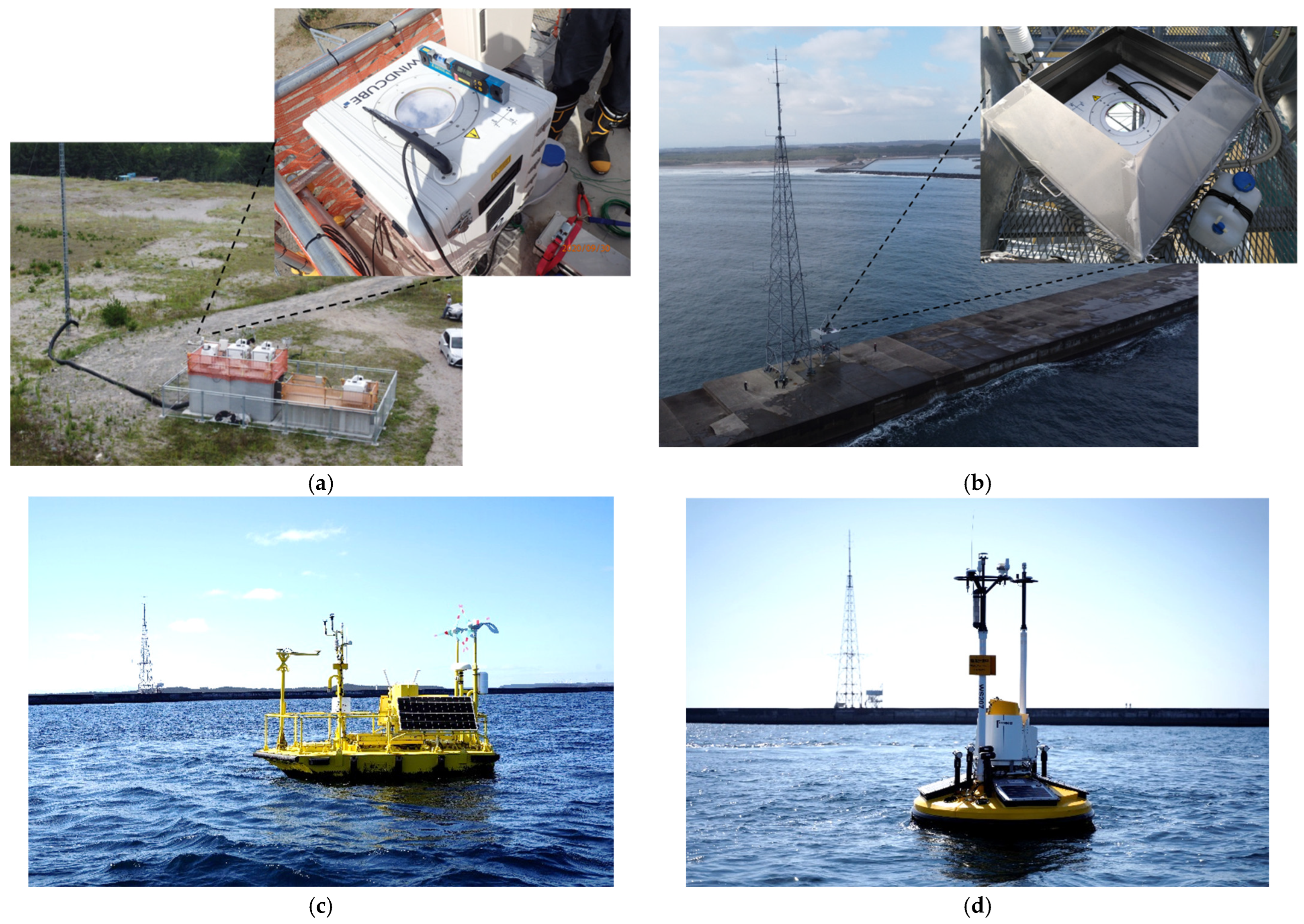
2.2. Observation
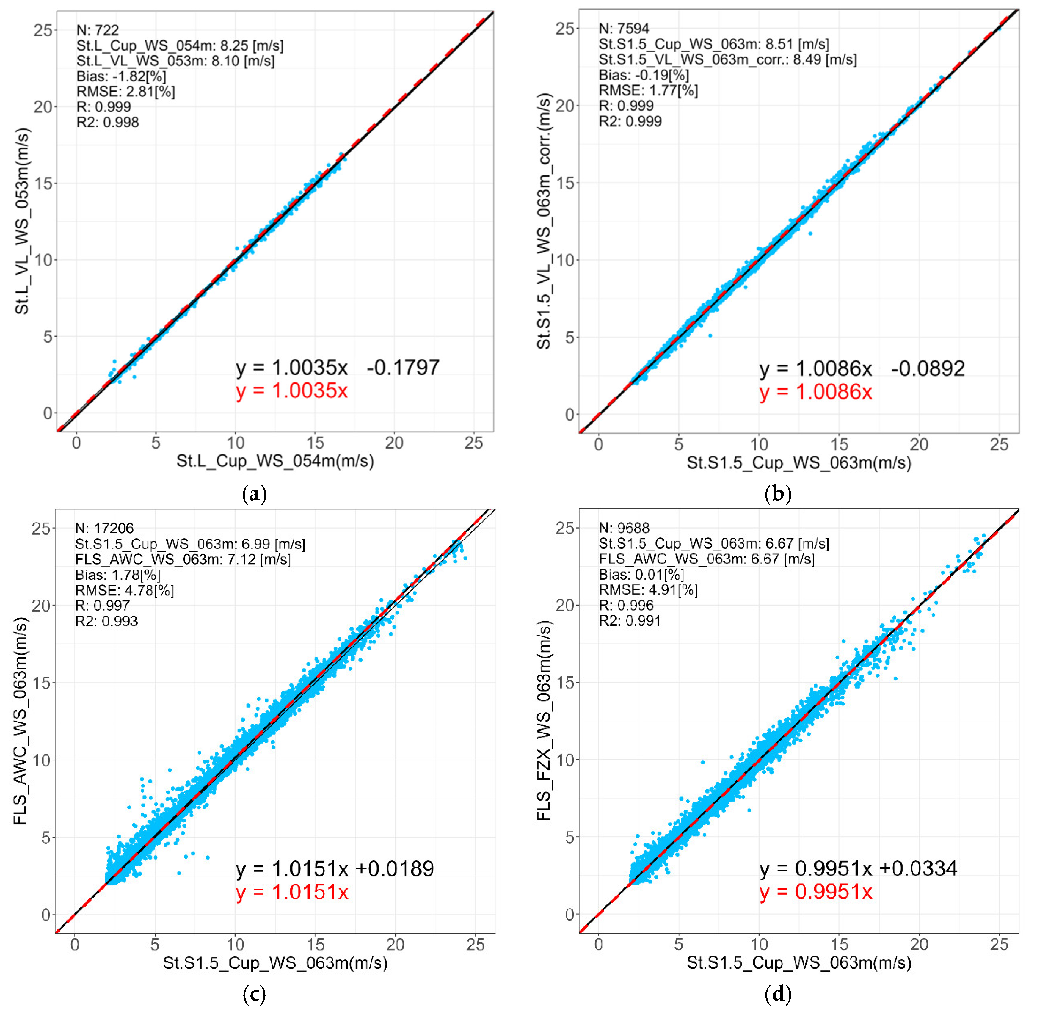
2.2.1. Wind Observation
2.2.2. Atmospheric Stability
3. Numerical Models
3.1. Overview of Models and Reference Settings
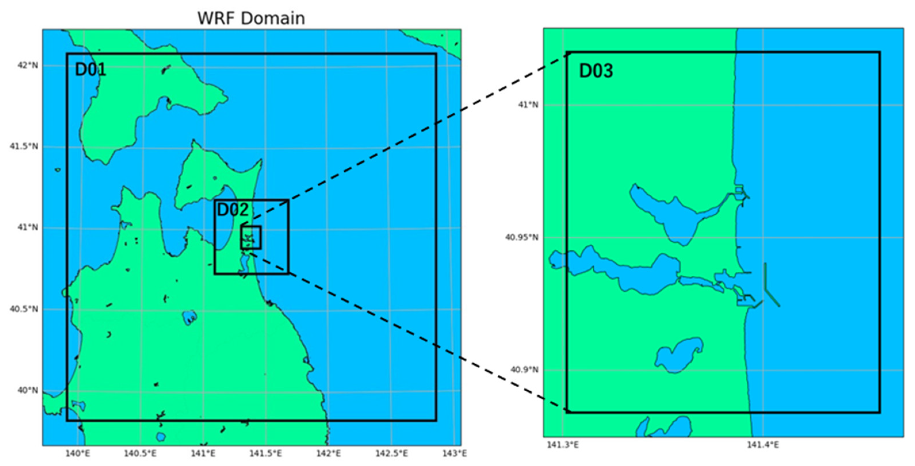
3.2. WRF
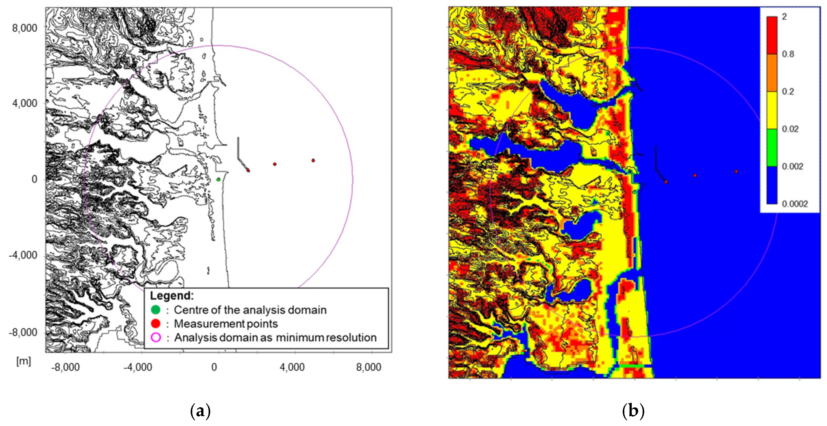
3.3. MASCOT
3.4. WAsP (WAsP-IBZ, WAsP-CFD)
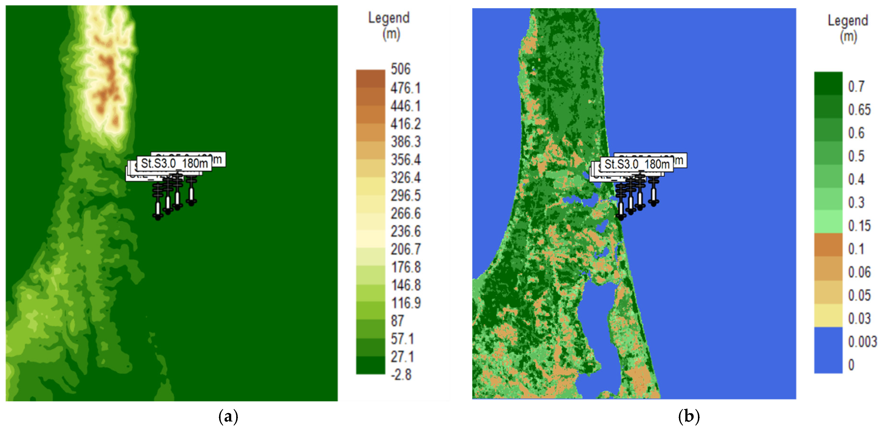
3.5. Meteodyn WT™ (Neutral, Unstable Condition)
- ➢
- Tree height was defined by roughness length values and the ratio (R) between tree height and roughness length (default R = 20).
- ➢
- Forest density directly affects the drag force term from forest effects (default: normal forest density) [52].
4. Results
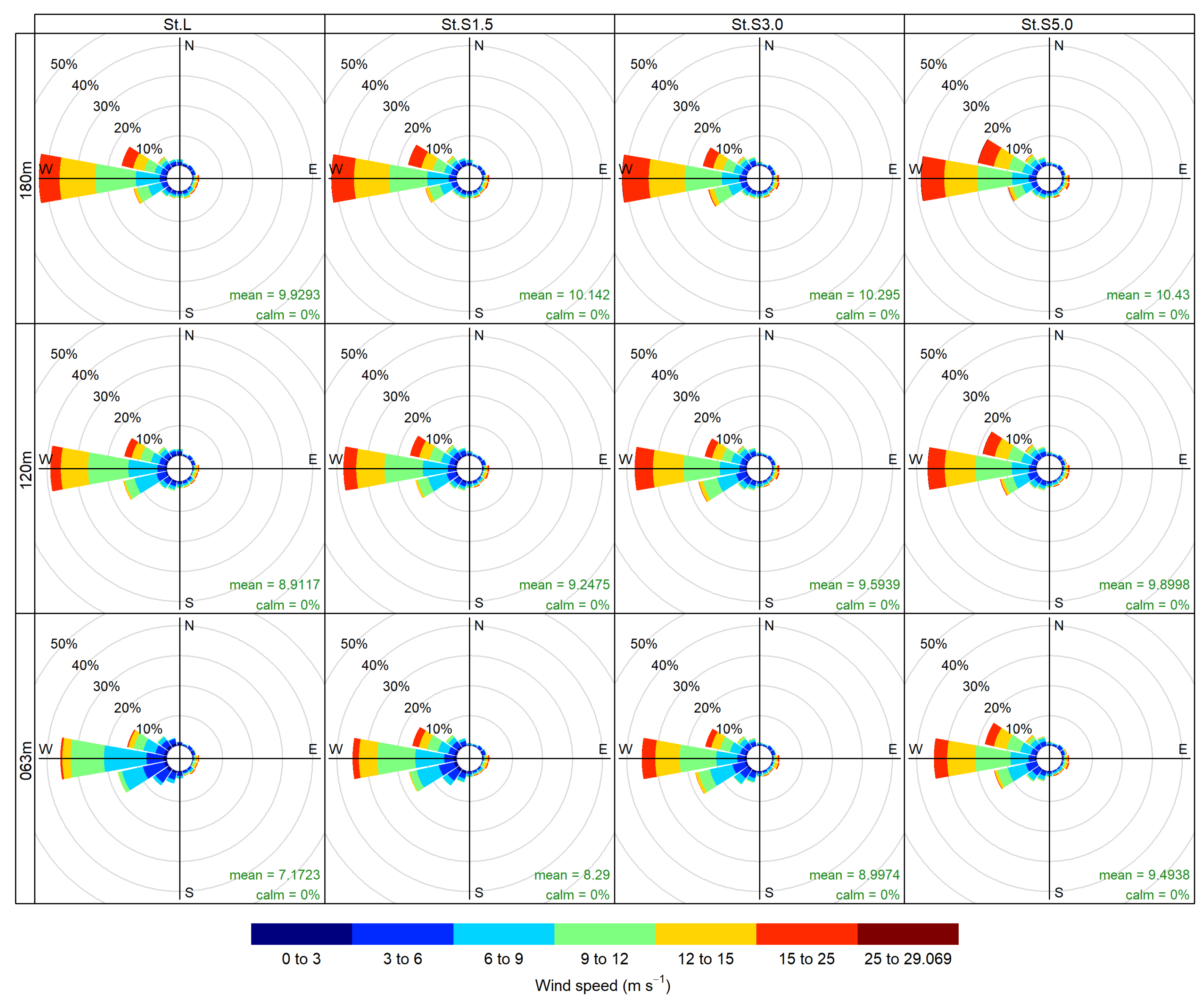
4.1. Observed Wind Conditions
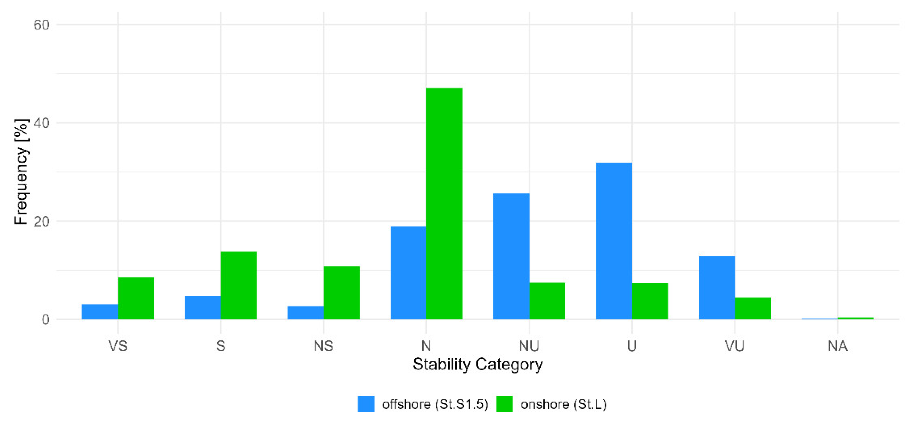
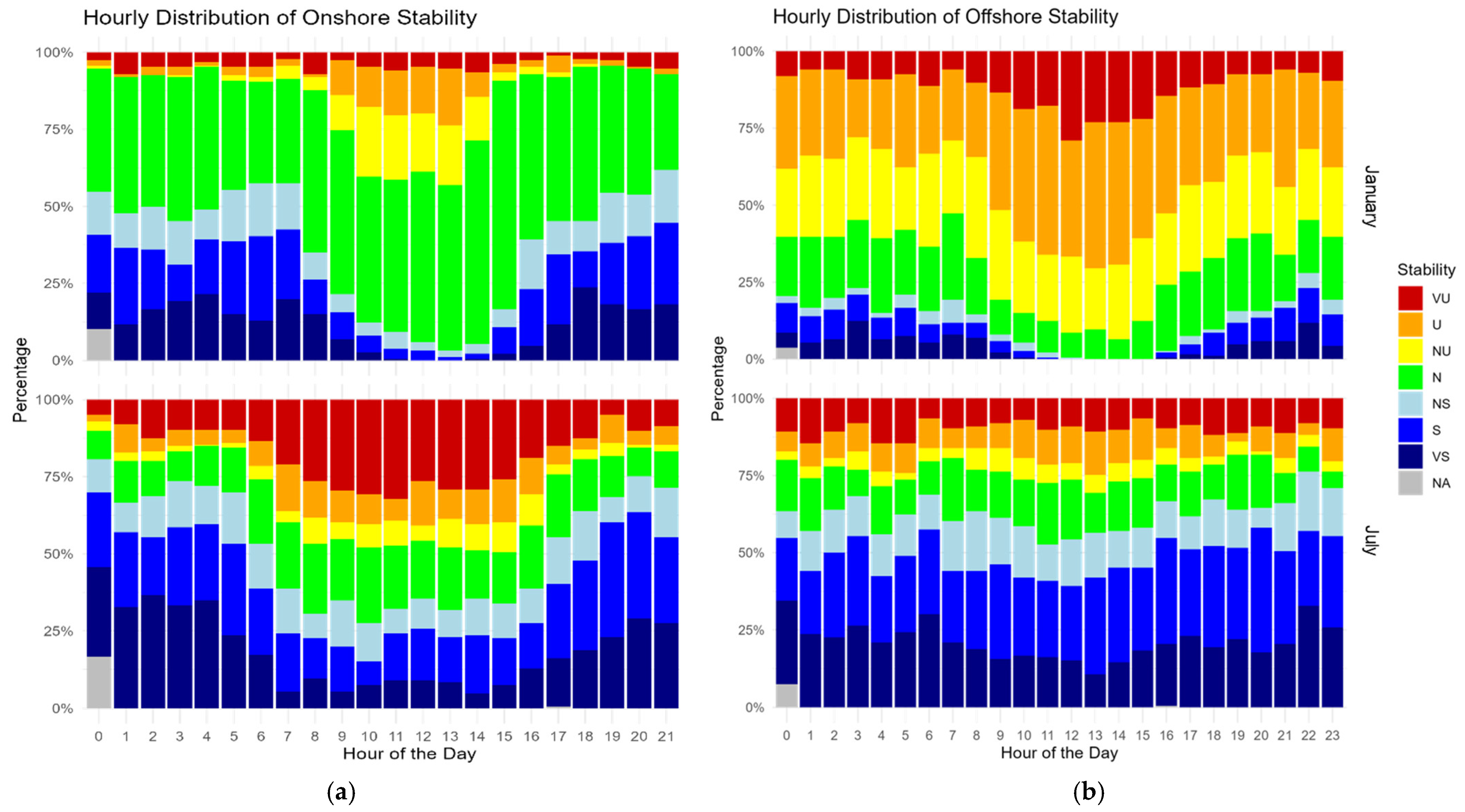
4.2. Observed Atmospheric Stability
4.3. Model Analysis
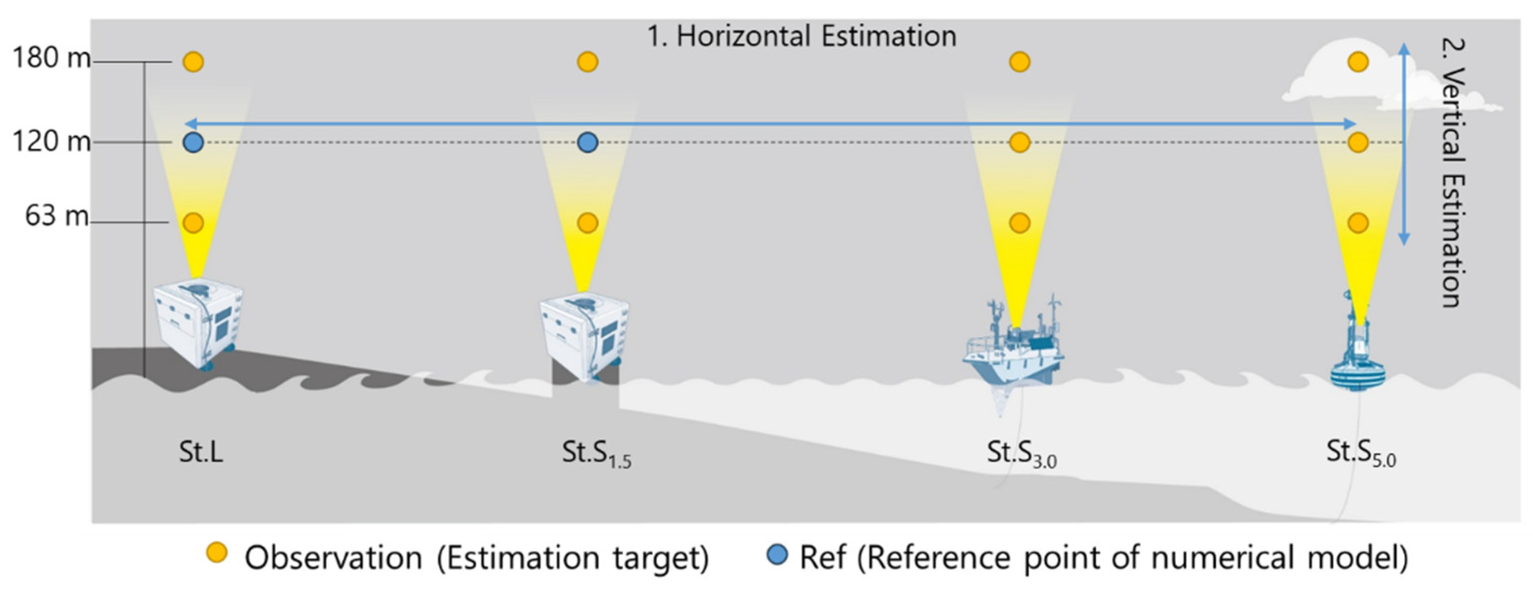
- Horizontal Estimation: Assessment of the estimation accuracy in the horizontal offshore direction at the same height (120 m) as the Ref.
- Vertical Estimation: Evaluation of the estimation accuracy in the vertical direction, including heights different from the Ref (63 and 180 m).
4.3.1. Horizontal Estimation Accuracy
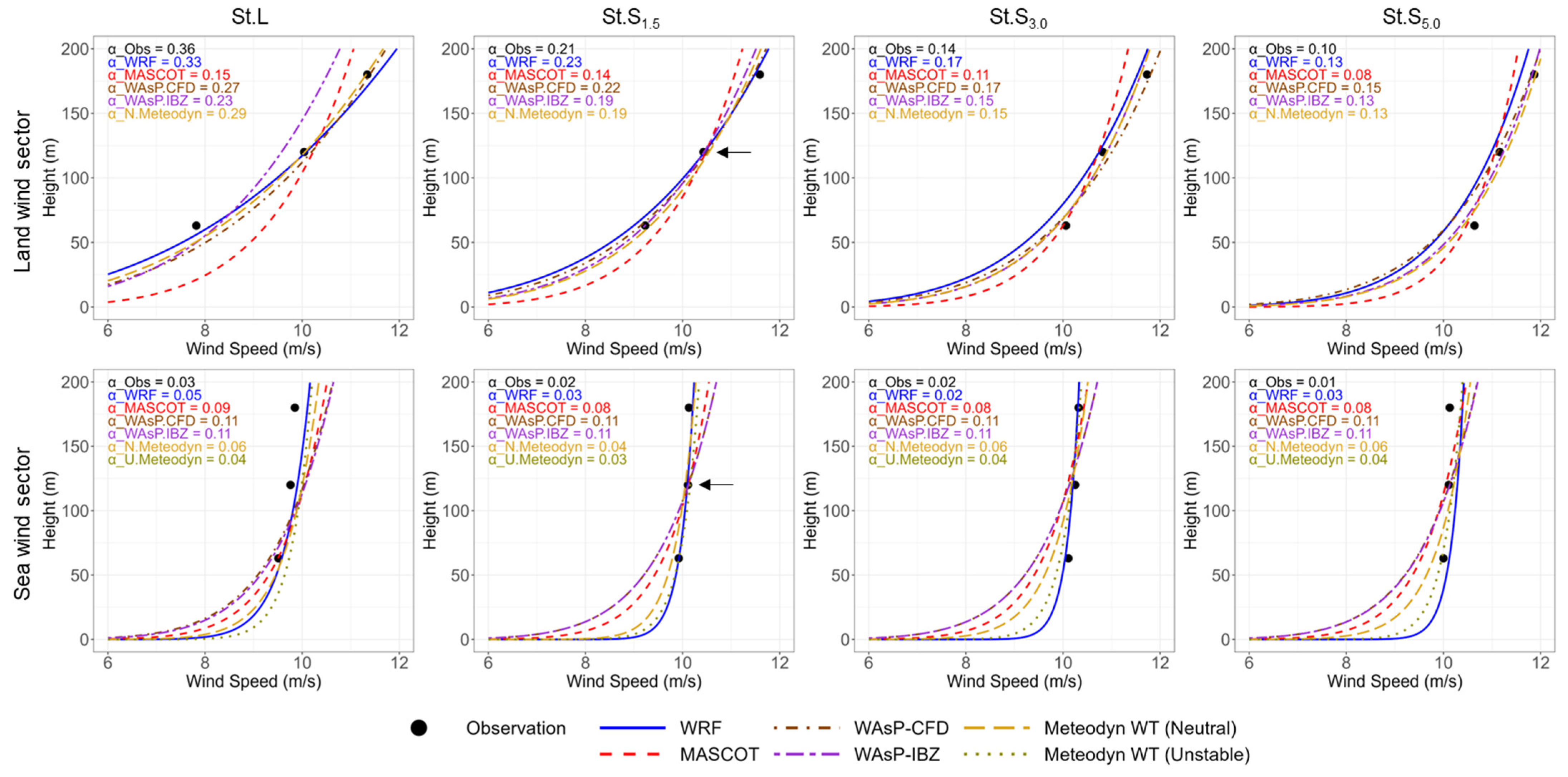
4.3.2. Vertical Estimation Accuracy
5. Discussion
5.1. Wind Characteristics and Influencing Mechanisms
5.2. Spatial and Temporal Variation of Atmospheric Stability
6. Conclusions
- Horizontal Estimation: Wind speed estimation accuracy in the offshore direction improved when using a nearshore reference (St.S1.5) instead of an onshore reference (St.L). Biases in the offshore area were generally within ±2.2% up to 5 km from the coast, indicating the practical advantage of using nearshore measurement locations.
- Vertical Estimation: Models incorporating atmospheric stability (e.g., WRF, Meteodyn WT™ under unstable conditions) better reproduced vertical wind profiles offshore. In contrast, models assuming neutral stability tended to overestimate wind shear, particularly under unstable stratification.
- Model Suitability by Sector: Sea-sector winds were better represented by models with thermodynamic treatments, while land-sector winds—predominantly neutral and mechanically influenced—showed less distinction across the models. However, residual thermal effects over sea surfaces impacted land-sector winds, suggesting that even nearshore modeling benefits from stability consideration.
- Atmospheric Stability Variability: Atmospheric stability exhibited significant spatial, temporal, and seasonal variability—particularly during winter—with neutral conditions frequently observed over land and unstable conditions prevailing offshore. These variations influenced the estimation of vertical wind shear and underscore the importance of using stability-aware models in coastal regions.
Author Contributions
Funding
Data Availability Statement
Acknowledgments
Conflicts of Interest
Abbreviations
| CFD | Computational fluid dynamics |
| FLS | Floating LiDAR system |
| LiDAR | Light detection and ranging |
| MASCOT | Microclimate Analysis System for Complex Terrain |
| MOL | Monin–Obukhov length |
| NEDO | New Energy and Industrial Technology Development Organization |
| RANS | Reynolds-averaged Navier–Stokes |
| SST | Sea surface temperature |
| VL | Vertical LiDAR |
| WAsP | Wind Atlas Analysis and Application Program |
| WRF | Weather Research and Forecasting |
References
- GWEC Global Wind REPORT 2024. 2024. Available online: https://img.saurenergy.com/2024/05/gwr-2024_digital-version_final-1-compressed.pdf (accessed on 27 May 2025).
- Ninos, E.; Lucas, M.; Ballantyne, J. Japanese Offshore Wind—Status and Recent Developments. Watson Farley & Williams Article. 2024. Available online: https://www.wfw.com/articles/japanese-offshore-wind-developments/ (accessed on 27 May 2025).
- Konagaya, M.; Ohsawa, T.; Inoue, T.; Mito, T.; Kato, H.; Kawamoto, K. Land–sea contrast of nearshore wind conditions: Case study in Mutsu-Ogawara. Sola 2021, 17, 234–238. [Google Scholar] [CrossRef]
- Evaluation of Site-Specific Wind Condition; Version 3; Measurement Procedures; MEASNET: Madrid, Spain, 2022.
- Skamarock, W.C.; Klemp, J.B.; Dudhia, J.; Gill, D.O.; Liu, Z.; Berner, J.; Wang, W.; Powers, J.G.; Duda, M.G.; Barker, D.M.; et al. A Description of the Advanced Research WRF Model Version 4; Tech. Note TN-556+STR; National Center for Atmospheric Research: Boulder, CO, USA, 2021; pp. 1–148. Available online: https://www.ecampmany.com/docs/cheatsheets/WRF.pdf (accessed on 27 May 2025).
- Misaki, T.; Ohsawa, T. Evaluation of LFM-GPV and MSM-GPV as input data for wind simulation. J. JWEA 2018, 42, 72–79. [Google Scholar] [CrossRef]
- Misaki, T. A Study on Improving the Accuracy of Coastal Wind Speeds Simulated by Mesoscale Model. Ph.D. Thesis, Kobe University, Kobe, Japan, 2020. Available online: https://hdl.handle.net/20.500.14094/D1007801 (accessed on 27 May 2025).
- Shimada, S.; Ohsawa, T.; Kogaki, T.; Steinfeld, G.; Heinemann, D. Effects of sea surface temperature accuracy on offshore wind resource assessment using a mesoscale model. Wind Energy 2015, 18, 1839–1854. [Google Scholar] [CrossRef]
- Ohsawa, T.; Ishigami, K.; Baba, Y.; Kawaguchi, K. Comparison of WRF-based methods for wind resource assessment at an offshore site. In Proceedings of the Twenty-Fifth International Ocean and Polar Engineering Conference, Kona, HI, USA, 21–26 June 2015. [Google Scholar]
- NEDO. The NEDO Offshore Wind Information System. Available online: https://appwdc1.infoc.nedo.go.jp/Nedo_Webgis/top.html (accessed on 27 May 2025).
- Ohsawa, T.; Uede, H.; Misaki, T.; Kato, M. Accuracy of WRF Simulations Used for Japanese Offshore Wind Resource Maps. In Proceedings of the International Conference on Energy and Meteorology, Bari, Italy, 27–29 June 2017; Available online: http://www.wemcouncil.org/ICEMs/ICEM2017_PRES/ICEM_20170629_1120_Sala_2_Ohsawa.pptx (accessed on 27 May 2025).
- Kato, M.; Ohsawa, T.; Uede, H.; Shimada, S. Verification of spatial characteristics of WRF-simulated wind speed in Japanese coastal waters. Proc. Jpn. Wind. Energy Symp. 2017, 39, 253–256. (In Japanese) [Google Scholar] [CrossRef]
- Misaki, T.; Ohsawa, T.; Konagaya, M.; Shimada, S.; Takeyama, Y.; Nakamura, S. Accuracy comparison of coastal wind speeds between WRF simulations using different input datasets in Japan. Energies 2019, 12, 2754. [Google Scholar] [CrossRef]
- Makridis, A.; Chick, J. Validation of a CFD model of wind turbine wakes with terrain effects. J. Wind Eng. Ind. Aerodyn. 2013, 123, 12–29. [Google Scholar] [CrossRef]
- Liu, Y.; Ishihara, T. Fatigue Failure Accident of Wind Turbine Tower in Taikoyama Wind Farm. In Proceedings of the EWEA2015, Paris, France, 17–20 November 2015. [Google Scholar]
- Kyokai, N.K. Wind Farm Certification Onshore Wind Power Plant Edition. Available online: https://www.classnk.or.jp/hp/pdf/authentication/renewableenergy/en/windfarm/NKRE-GL-WFC01_March2023_Eng_20230331.pdf (accessed on 27 May 2025).
- NEDO. Offshore Wind Measurement Guidebook. 2023. Available online: https://www.nedo.go.jp/library/fuukyou_kansoku_guidebook.html (accessed on 27 May 2025).
- Shimada, S.; Kogaki, T.; Konagaya, M.; Mito, T.; Araki, R.; Ueda, Y.; Ohsawa, T. Validation of near-shore wind measurements using a dual scanning light detection and ranging system. Wind Energy 2022, 25, 1555–1572. [Google Scholar] [CrossRef]
- DTU. WAsP Software. Available online: https://www.wasp.dk/ (accessed on 27 May 2025).
- Lange, B.; Højstrup, J. Evaluation of the wind-resource estimation program WAsP for offshore applications. J. Wind Eng. Ind. Aerodyn. 2001, 89, 271–291. [Google Scholar] [CrossRef]
- Bechmann, A. WAsP CFD A New Beginning in Wind Resource Assessment; Technical Report; Riso National Laboratory: Roskilde, Denmark, 2012. Available online: https://www.wasp.dk/software/wasp-cfd (accessed on 27 May 2025).
- Konagaya, M.; Ohsawa, T.; Mito, T.; Misaki, T.; Maruo, T.; Baba, Y. Estimation of nearshore wind conditions using onshore observation data with computational fluid dynamic and mesoscale models. Resources 2022, 11, 100. [Google Scholar] [CrossRef]
- Takakuwa, S.; Uchida, T. Improvement of airflow simulation by refining the inflow wind direction and applying atmospheric stability for onshore and offshore wind farms affected by topography. Energies 2022, 15, 5050. [Google Scholar] [CrossRef]
- López, G.; Arboleya, P.; Núñez, D.; Freire, A.; López, D. Wind resource assessment and influence of atmospheric stability on wind farm design using Computational Fluid Dynamics in the Andes Mountains, Ecuador. Energy Convers. Manag. 2023, 284, 116972. [Google Scholar] [CrossRef]
- Jimenez, B.; Durante, F.; Lange, B.; Kreutzer, T.; Tambke, J. Offshore wind resource assessment with WAsP and MM5: Comparative study for the German Bight. Wind Energy 2007, 10, 121–134. [Google Scholar] [CrossRef]
- Uchida, T.; Li, G. Comparison of RANS and LES in the prediction of airflow field over steep complex terrain. Open J. Fluid Dyn. 2018, 8, 286–307. [Google Scholar] [CrossRef]
- Beaucage, P.; Brower, M.C.; Tensen, J. Evaluation of four numerical wind flow models for wind resource mapping. Wind Energ. 2014, 17, 197–208. [Google Scholar] [CrossRef]
- Ohsawa, T.; Shimada, S.; Kogaki, T.; Iwashita, T.; Konagaya, M.; Araki, R.; Imamura, H. Progress of NEDO project “Bottom fixed offshore wind farm development support project (Establishment of offshore wind resource assessment method)”. Proc. Jpn. Wind. Energy Symp. 2020, 42, 136–139. (In Japanese) [Google Scholar]
- Kobe University. MOC, Mutsu-Ogawara Offshore Wind Observation Test Site. Available online: https://mo-testsite.com/ (accessed on 27 May 2025).
- Uchiyama, S.; Ohsawa, T.; Asou, H.; Konagaya, M.; Misaki, T.; Araki, R.; Hamada, K. Accuracy verification of multiple floating LiDARs at the Mutsu-Ogawara site. Energies 2024, 17, 3164. [Google Scholar] [CrossRef]
- Wind Cube Vertical Profiler. Available online: https://www.vaisala.com/en/products/wind-energy-windcube (accessed on 27 May 2025).
- AXYS. WindSentinel. Available online: https://axys.com/flidar-windsentinel/ (accessed on 27 May 2025).
- Kelberlau, F.; Mann, J. Quantification of motion-induced measurement error on floating lidar systems. Atmos. Meas. Tech. 2022, 15, 5323–5341. [Google Scholar] [CrossRef]
- ZX Lidars. ZX300M. Available online: https://www.zxlidars.com/wind-lidars/zx-300m/ (accessed on 27 May 2025).
- Uchiyama, S.; Ohsawa, T.; Asou, H.; Konagaya, M.; Misaki, T.; Araki, R.; Hamada, K. Empirical Motion Compensation for Turbulence Intensity Measurement by Floating LiDARs. Energies 2025, 18, 2931. [Google Scholar] [CrossRef]
- Carbon Trust. Offshore Wind Accelerator (OWA), Road Map for the Commercial Acceptance of Floating LIDAR Technology. 2018. Available online: https://ctprodstorageaccountp.blob.core.windows.net/prod-drupal-files/documents/resource/public/Roadmap%20for%20Commercial%20Acceptance%20of%20Floating%20LiDAR%20REPORT.pdf (accessed on 27 May 2025).
- Lange, B.; Larsen, S.; Højstrup, J.; Barthelmie, R. The influence of thermal effects on the wind speed profile of the coastal marine boundary layer. Boundary Layer Meteorol. 2004, 112, 587–617. [Google Scholar] [CrossRef]
- Gryning, S.E.; Batchvarova, E.; Brümmer, B.; Jørgensen, H.; Larsen, S. On the extension of the wind profile over homogeneous terrain beyond the surface boundary layer. Boundary Layer Meteorol. 2007, 124, 251–268. [Google Scholar] [CrossRef]
- UCAR. Weather Research & Forecasting Model (WRF). Available online: https://www.mmm.ucar.edu/models/wrf (accessed on 27 May 2025).
- Ishihara, T.; Hibi, K. Numerical study of turbulent wake flow behind a three-dimensional steep hill. Wind Struct. 2002, 5, 317–328. [Google Scholar] [CrossRef]
- Ishihara, T.; Yamaguchi, A.; Fujino, Y. A Nonlinear model for predictions of turbulent flow over steep terrain. In Proceedings of the World Wind Energy Conference and Exhibition, Berlin, Germany, 2–6 July 2002; pp. 1–4. [Google Scholar]
- Aqua net. MASCOT. Available online: https://www.aquanet21.co.jp/mascot/ (accessed on 27 May 2025).
- Mortensen, N.G. Wind Resource Assessment Using the WAsP Software; DTU Wind Energy E No. 0135; Technical University of Denmark: Roskilde, Denmark, 2016; Available online: https://backend.orbit.dtu.dk/ws/portalfiles/portal/140943898/Wind_resource_assessment_using_the_WAsP_software_DTU_Wind_Energy_E_0135_.pdf (accessed on 27 May 2025).
- Meteodyn. Meteodyn WT. Available online: https://meteodyn.com/sectors/onshore-and-offshore-wind-power/meteodyn-universe-wind-farm-development-software/meteodyn-wt-wind-resource-assessment-software/ (accessed on 27 May 2025).
- Pieterse, J.E.; Harms, T.M. CFD investigation of the atmospheric boundary layer under different thermal stability conditions. J. Wind Eng. Ind. Aerodyn. 2013, 121, 82–97. [Google Scholar] [CrossRef]
- Maruo, T.; Ohsawa, T.; Takakuwa, S.; Hemmi, C.; Watanabe, K.; Hasegawa, S.; Kouso, K.; Shirai, K. Validation of WRF and Vector Equation Method for Nearshore Wind Resource assessment: A Comparison of Accuracy Depending on Input Point Location and Number of Points. Proc. Jpn. Wind. Energy Symp. 2023, 45, 9–12. (In Japanese) [Google Scholar] [CrossRef]
- JMA. Numerical Weather Prediction Activities. Available online: https://www.jma.go.jp/jma/en/Activities/nwp.html (accessed on 27 May 2025).
- Shimizu, Y.; Ohsawa, T.; Shimada, S. Accuracy validation of offshore wind simulation using WRF with the new SST dataset IHSST. Proc. Jpn. Wind. Energy Symp. 2018, 40, 167–170. (In Japanese) [Google Scholar] [CrossRef]
- Murakami, H. Accuracy estimation of digital map series data sets published by the Geographical Survey Institute. Geoinformatics 1995, 6, 59–64. [Google Scholar] [CrossRef] [PubMed]
- The Ministry of Land, Infrastructure, Transport and Tourism. Data, L.U.M. Available online: http://nlftp.mlit.go.jp/ksj/gml/datalist/KsjTmplt-L03-b.html (accessed on 27 May 2025).
- EMD International. Chapter 3. WindPRO Knowledge Base—WindPRO 3.6 User Manual. 2022. Available online: https://help.emd.dk/knowledgebase/content/windPRO3.6/c3-UK_windPRO3.6_ENERGY.pdf (accessed on 27 May 2025).
- Leonard, E.; Li, R.; Tromeur, E.; Dupont, M.; Martellozzo, G.; Gaussorgues, A.; Koutsioumpas, S.; Akcakaya, M. New CFD caliburation methodology for wind resource assessment in highly forested area. In Proceedings of the WindEurope, Bilbao, Spain, 20–22 March 2024; Available online: https://www.youtube.com/watch?v=KRejPD9qVy4 (accessed on 27 May 2025).
- Copernicus Land Monitoring Service. Corine Land Cover (CLC) 2018; Version 20b2—100 m Raster Data; European Environment Agency: Copenhagen, Denmark, 2019. Available online: https://land.copernicus.eu (accessed on 27 May 2025).
- Li, R.; Leonard, E.; Tromeur, E. Comparison of Three Methods in Atmospheric Stratification Determination. In Proceedings of the WindEurope Brussels, Brussels, Belgium, 23–24 June 2022. [Google Scholar]


| Site | St.L | St.S1.5 |
|---|---|---|
| VL Model | Windcube V2.1 | |
| Implementer | Vaisala | |
| Number of observation heights | 12 | |
| Observation height from mean sea level 1 | 43, 50, 59, 63, 80, 100, 120, 140, 160, 180, 200, and 250 m 2 | 50, 59, 80, 63, 66, 80, 100, 120, 140, 160, 180, 200, and 250 m |
| Measuring range | Speed: 0–55 m/s | |
| Direction: 0–360° | ||
| Measuring accuracy | Speed: 0.1 m/s | |
| Direction: 2° | ||
| Averaging time | 10 min | |
| Site | St.S3.0 | St.S5.0 |
| FLS model | WindSentinel | SEAWATCH |
| FLS implementer | AXYS | Fugro |
| VL model | Windcube V2.0 | ZX300M |
| VL implementer | Vaisala (Leosphere) | ZX LiDAR, |
| Number of observation heights | 12 | 13 |
| Observation height from mean sea level 1 | 43, 50, 59, 63, 80, 100, 120, 140, 160, 180, 200, and 250 m | 50, 59, 80, 63, 66, 80, 100, 120, 140, 160, 180, 200, and 250 m |
| Averaging time | 10 min | |
| L (m) | Atmospheric Stability Category |
|---|---|
| –50 < L ≤ 0 | Very Unstable |
| –200 < L ≤ –50 | Unstable |
| –500 < L ≤ –200 | Near Unstable |
| L ≤ –500, 500 ≤ L | Neutral |
| 200 < L ≤ 500 | Near Stable |
| 50 < L ≤ 200 | Stable |
| 0 < L ≤ 50 | Very Stable |
| Model | Advanced Research WRF ver.4.1.2 |
| Period | 1 December 2021–31 March 2022 JST |
| Input data | Met.: Japan Meteorological Agency Local Forecast Model (1-hourly, 0.04° × 0.05° at pressure level and 0.025° × 0.020° at surface level) Soil: NCEP FNL (6-hourly, 1° × 1°) SST: Met Office OSTIA (Daily, 0.05° × 0.05°) |
| Terrain data | Elevation: METI, NASA ASTER GDEM Land use: MLIT, NLNI land use subdivision mesh |
| Grids | Domain 1: 2.5 km × 2.5 km (100 × 100 grids) Domain 2: 0.5 km × 0.5 km (100 × 100 grids) Domain 3: 0.1 km × 0.1 km (130 × 150 grids) |
| Vertical levels | 40 layers (surface to 100 hPa) |
| Physics options | Shortwave process: Dudhia scheme Longwave process: Rapid Radiative Transfer Model scheme Cloud microphysics process: Ferrier (new Eta) scheme PBL process: Mellor–Yamada–Janic (Eta operational) scheme Surface layer process: Monin–Obukhov (Janic Eta) scheme Land-surface process: Noah Land Surface Model scheme Cumulus parameterization: Kain–Fritsch (new Eta) scheme (Domain 1) |
| FDDA | Domain 1: Enabled (U, V, T, Q) Domain 2, 3: Enabled (U, V, T, Q), excluding the interior of PBL |
| Model | MASCOT Ver.5.1a |
| Center of the calculation domain | 40° 55′ 3.25″ N, 141° 23′ 32.68″ E (Tokyo Datum) |
| Elevation data | GSI 50 m grid digital elevation model data |
| Ground roughness | Based on the 100 m mesh land use data |
| Size of the calculation domain | 18 km × 18 km |
| Wind direction | 16 directions |
| Minimum horizontal resolution | 25 m |
| Minimum vertical resolution | 5 m |
| Calculation domain as minimum resolution | Within a 7000 m radius |
| Number of mesh | 29,261,232 |
| Type | Roughness Length (m) |
|---|---|
| Rice field (Tanbo) | 0.03 |
| Field | 0.1 |
| Orchard | 0.2 |
| Other wood field | 0.1 |
| Forests | 0.8 |
| Wasteland | 0.03 |
| High buildings | 1 |
| Low buildings | 0.4 |
| Transportation area | 0.1 |
| Other area | 0.03 |
| Lakes and ponds | 0.0002 |
| River A: Does not include artificial land use in river areas | 0.001 |
| River B: Artificial land use in riverbeds | 0.001 |
| Beach | 0.03 |
| Sea | 0.0002 |
| Model | WAsP-IBZ (WAsP Version 12) |
|---|---|
| Azimuth resolution in BZ model | 5° |
| Decay length for roughness area size | 10,000 m |
| Default background roughness area size | 0.03 m |
| Height of inversion in BZ model | 1000 m |
| Max. interpolation radius in BZ model | 20,000 m |
| Max number of roughness changes/sector | 10 |
| Max. rms error in log(roughness) analysis | 0.3 |
| Softness of inversion in BZ model | 1 |
| Sub-sectors in roughness map analysis | 9 |
| Width of coastal zone | 10,000 m |
| Wind direction | 16 directions |
| Model | WAsP-CFD Version: 1.11.2.7 |
|---|---|
| Number of calculation domain | Four tile domains |
| Size of calculation domain | 4 km × 4 km in each domain |
| Calculation domain as minimum resolution | 2 km × 2 km in each domain |
| Wind direction | 36 directions |
| Mean resolution horizontal/vertical | 20.7/5 m |
| Domain height/diameter | 14/34 km |
| Model | Meteodyn WT™ Version: 1.9 |
|---|---|
| Center of the calculation domain | 40°55′29.4″ N, 141°25′5.6″ E (WGS84) |
| Site radius | 13 km |
| Elevation data | Nasadem: 30 m resolution |
| Roughness data | Copernicus, 2019 [53] 100 m resolution |
| CFD minimum horizontal resolution | 25 m |
| CFD minimum vertical resolution | 4 m |
| Number of directions | 20 |
| Number of cells in the mesh | Direction 90 deg: 4,046,112 Direction 270 deg: 3,933,720 |
Disclaimer/Publisher’s Note: The statements, opinions and data contained in all publications are solely those of the individual author(s) and contributor(s) and not of MDPI and/or the editor(s). MDPI and/or the editor(s) disclaim responsibility for any injury to people or property resulting from any ideas, methods, instructions or products referred to in the content. |
© 2025 by the authors. Licensee MDPI, Basel, Switzerland. This article is an open access article distributed under the terms and conditions of the Creative Commons Attribution (CC BY) license (https://creativecommons.org/licenses/by/4.0/).
Share and Cite
Konagaya, M.; Ohsawa, T.; Itoshima, Y.; Kambayashi, M.; Leonard, E.; Tromeur, E.; Misaki, T.; Shintaku, E.; Araki, R.; Hamada, K. Estimation of Wind Conditions in the Offshore Direction Using Multiple Numerical Models and In Situ Observations. Energies 2025, 18, 3000. https://doi.org/10.3390/en18113000
Konagaya M, Ohsawa T, Itoshima Y, Kambayashi M, Leonard E, Tromeur E, Misaki T, Shintaku E, Araki R, Hamada K. Estimation of Wind Conditions in the Offshore Direction Using Multiple Numerical Models and In Situ Observations. Energies. 2025; 18(11):3000. https://doi.org/10.3390/en18113000
Chicago/Turabian StyleKonagaya, Mizuki, Teruo Ohsawa, Yuki Itoshima, Masaki Kambayashi, Edouard Leonard, Eric Tromeur, Takeshi Misaki, Erika Shintaku, Ryuzo Araki, and Kohei Hamada. 2025. "Estimation of Wind Conditions in the Offshore Direction Using Multiple Numerical Models and In Situ Observations" Energies 18, no. 11: 3000. https://doi.org/10.3390/en18113000
APA StyleKonagaya, M., Ohsawa, T., Itoshima, Y., Kambayashi, M., Leonard, E., Tromeur, E., Misaki, T., Shintaku, E., Araki, R., & Hamada, K. (2025). Estimation of Wind Conditions in the Offshore Direction Using Multiple Numerical Models and In Situ Observations. Energies, 18(11), 3000. https://doi.org/10.3390/en18113000