Multi-Objective Time-Domain Coupled Feasible Region Construction Method for Virtual Power Plant Considering Global Stability

Abstract

Constructing a new power system with renewable energy as the main component requires an in-depth exploration of the regulation potential of massive, distributed flexibility resources within distribution networks. This approach aims to enhance the grid’s balancing capabilities. Virtual Power Plants can effectively aggregate flexibility resources, but the massive scale and heterogeneous nature of distributed resources pose challenges in assessing the regulation capabilities of the aggregated entity. In this paper, a feasible region solution model for Virtual Power Plants is established based on the vertex search method. Furthermore, by introducing the principles of Lyapunov stability analysis, a multi-objective time–domain coupled feasible region construction method for VPPs with global stability considerations is proposed. Through case study analysis, the boundaries of the VPP’s regulation capability and the time–neighborhood feasible regions characterized by the proposed method exhibit better full-time output stability and are more aligned with practical needs.

1. Introduction

In recent years, with the proposal and promotion of China’s “dual carbon” goals, distributed renewable energy has become increasingly prevalent [1]. The volatility and uncertainty of these resources present new challenges to the safe and stable operation of power systems [2,3,4]. In the new power system being developed in China, the distribution network layer encompasses a massive amount of distributed energy resources (DERs). By aggregating these distributed resources, it is possible to create a virtual power plant (VPP) that can be managed by grid operators. This approach is crucial for supporting the efficient utilization of distributed renewable energy, improving grid regulation capabilities, and ensuring the high-quality operation of the power system [5]. However, the dispersed and heterogeneous characteristics of distributed flexible resources [6] present considerable difficulties for the aggregation of these resources into a VPP and for assessing their regulation capabilities. Consequently, accurately and efficiently evaluating and characterizing the feasible regulation power range of a VPP has emerged as a key research topic.

Current research predominantly determines the power-feasible region of a VPP as the projection of the feasible region onto the P-Q plane at a single moment [7], the relationship of active power output between different connection nodes at a single moment [8,9], and the output boundaries and virtual state-of-charge boundaries over multiple moments [10,11,12,13]. Ref. [14] employs an inscribed hyperbox-based aggregated flexibility projection method to characterize the day-ahead multi-period peak load regulation domain of a VPP that aggregates distributed electricity and hydrogen resources. By considering the integration of electricity and hydrogen, this approach enhances the total power range and net income. Ref. [15] constructs a VPP aggregation model that takes into account DER network constraints and temporal coupling constraints. Based on a two-stage robust optimization model, it proposes an aggregation method under uncertainty scenarios and characterizes the P-Q feasible region of the VPP. In Ref. [16], Brouwer’s fixed-point theorem is applied to the second-order Taylor expansion of the nonlinear Dist-flow equations. This application allows for the construction of linear constraints that serve to internally approximate the Alternating Current (AC) feasible region for power transmission. The study then verifies the effectiveness of this approach by employing a vertex search method on an IEEE 33-node test system. Ref. [17] combines a data-driven approach with a distributed robust optimization model to propose a time-varying feasible domain evaluation method across multiple periods. This significantly improves computational efficiency and accuracy. Ref. [18] proposes a boundary contraction method based on high-dimensional polytopes to characterize the multi-period output and ramping boundaries of a VPP, and it equivalently models this as a combination of virtual energy storage and a virtual generator. Ref. [19] focuses on coupled constraint models such as the ramping constraints of gas turbines in smart distribution networks. It transforms the vertex search problem into a min–max bi-level progressive vertex search problem, significantly improving computational efficiency compared to the original vertex search method. This has substantial methodological implications for solving the feasible region of VPPs. Ref. [20] focuses on a VPP with decoupled electricity and heat, proposing a virtual energy storage (VES) modeling method for electric and thermal demand response. It introduces the Minkowski sum to represent the VES power range as an aggregated low-dimensional flexibility region, effectively improving the economic efficiency and carbon reduction of the VPP. Ref. [21] proposes a feasible region projection method based on a two-stage robust optimization model. It reformulates the dynamic economic robust scheduling model equivalently into a single-level linear programming model. This model can be effectively solved while ensuring the optimality of the solution, laying the methodological foundation for characterizing the robust feasible region of a VPP.

In summary, existing studies predominantly focus on evaluating the P-Q safe operating power region of a VPP at a single time period or the output and ramping upper bounds of a VPP over multiple periods. Fewer studies accurately characterize the output relationships between adjacent time periods. Additionally, due to the limited consideration of the impact of single-time-period feasibility region characterization on other time periods in current research, this results in an inability to fully assess the potential regulation capacity brought by other time periods (without considering temporal coupling constraints) or significant deviations between the full-time output and original power operating points near the feasibility region boundary (considering temporal coupling constraints but not the impact of single-time-period feasibility region characterization on other time periods). Therefore, there is an urgent need to research methods for constructing a multi-objective time–domain coupled feasible region for VPPs that considers global stability. Based on the above research needs, this paper introduces Lyapunov stability theory. During the process of characterizing the VPP feasibility region, we construct a full-time output stability index for VPPs to control the deviation between full-time output and original operating power points. Based on this, we propose a method for constructing a multi-objective time–domain coupled feasibility region for VPPs considering global stability. The proposed method ensures full-time output stability of VPPs while accurately characterizing the temporal coupling feasibility region, promoting the efficient participation of VPPs in China’s electricity market, and accelerating the development of new power systems.

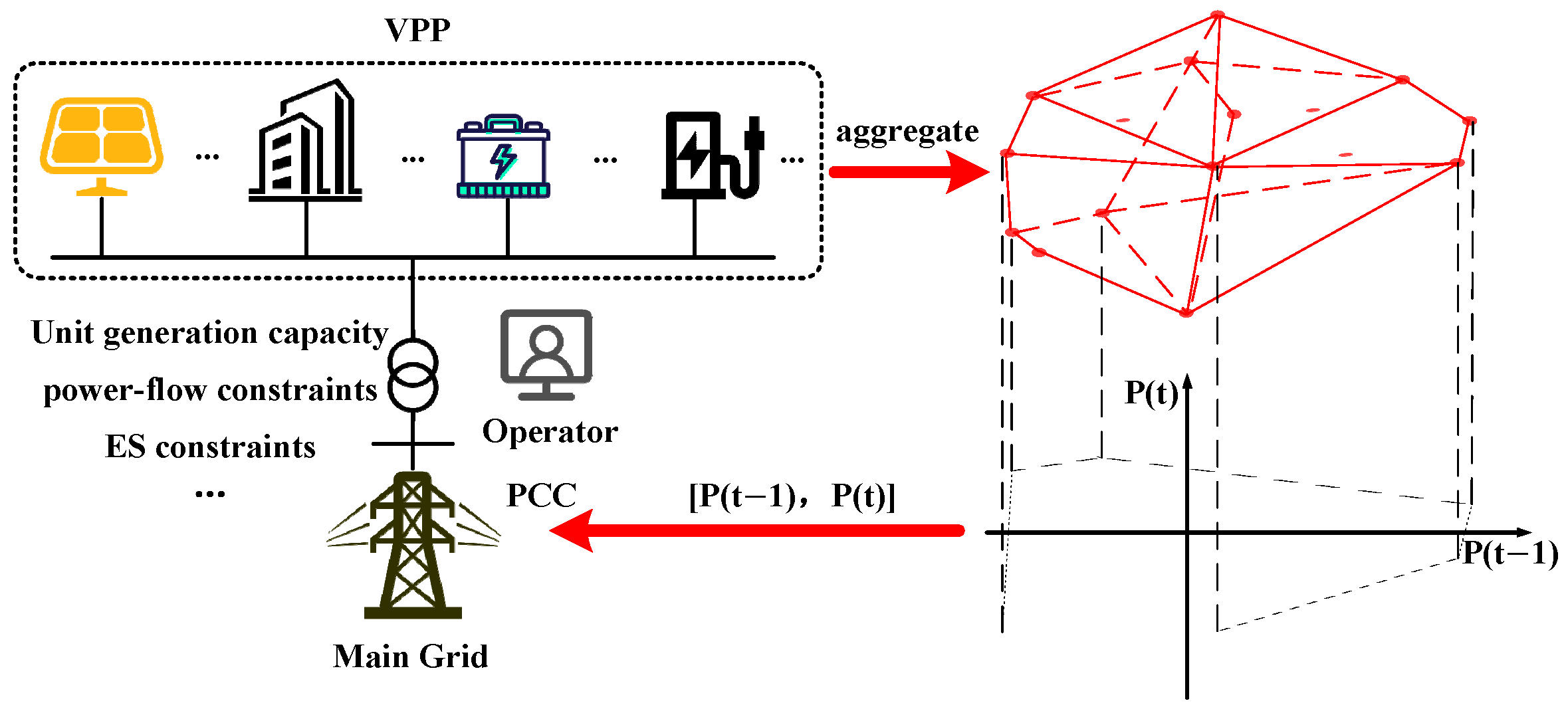
First, this paper cites Reference [14] to determine the feasible region of a VPP as the projection of its high-dimensional space aggregate onto the active power in adjacent time periods. 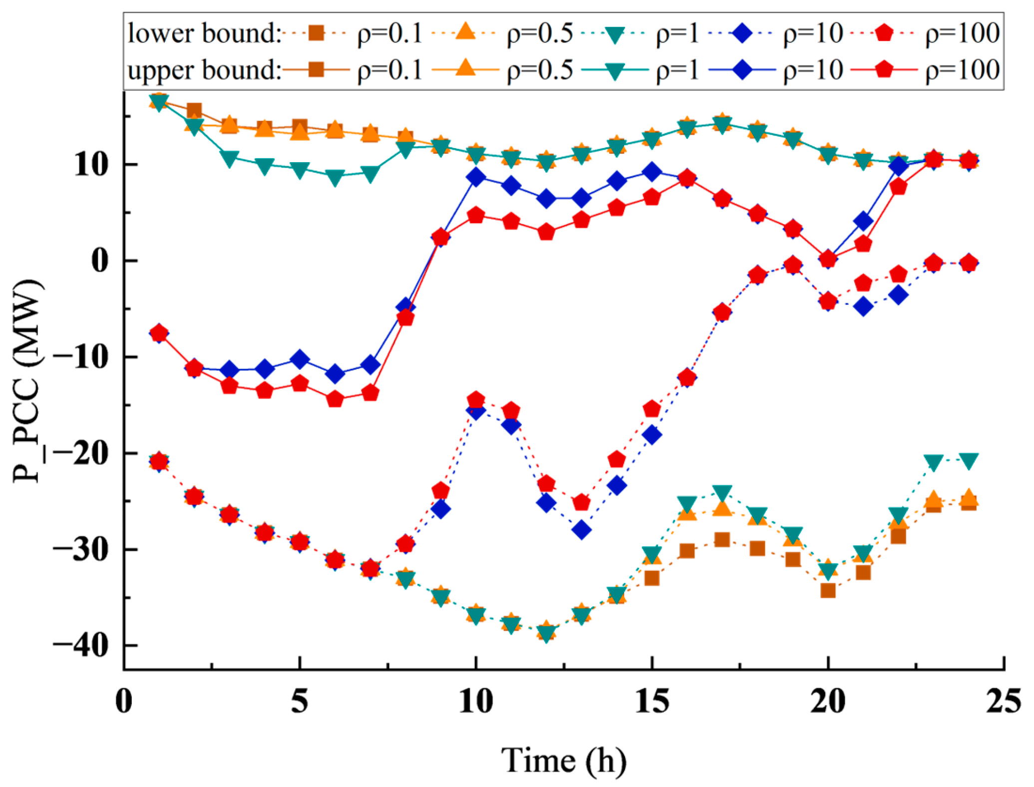The resulting temporal coupling feasibility region of the VPP not only represents the upper and lower limits of VPP output for specific time periods but also determines the upper and lower limits of ramping capability to the next time period based on the current operating power, as shown in Figure 1; Then, based on the principles of Lyapunov stability analysis, this paper proposes a global stability index to characterize the output stability of VPPs. Combining this with the method for characterizing the feasible region of VPPs, the paper introduces a multi-objective time–domain coupled feasible region construction method that considers global stability. Finally, this paper applies the vertex search method to characterize the output boundaries and active power-feasible region of adjacent time periods for a VPP aggregated on the IEEE 33-bus standard distribution network system, and it verifies the feasibility of the proposed method.

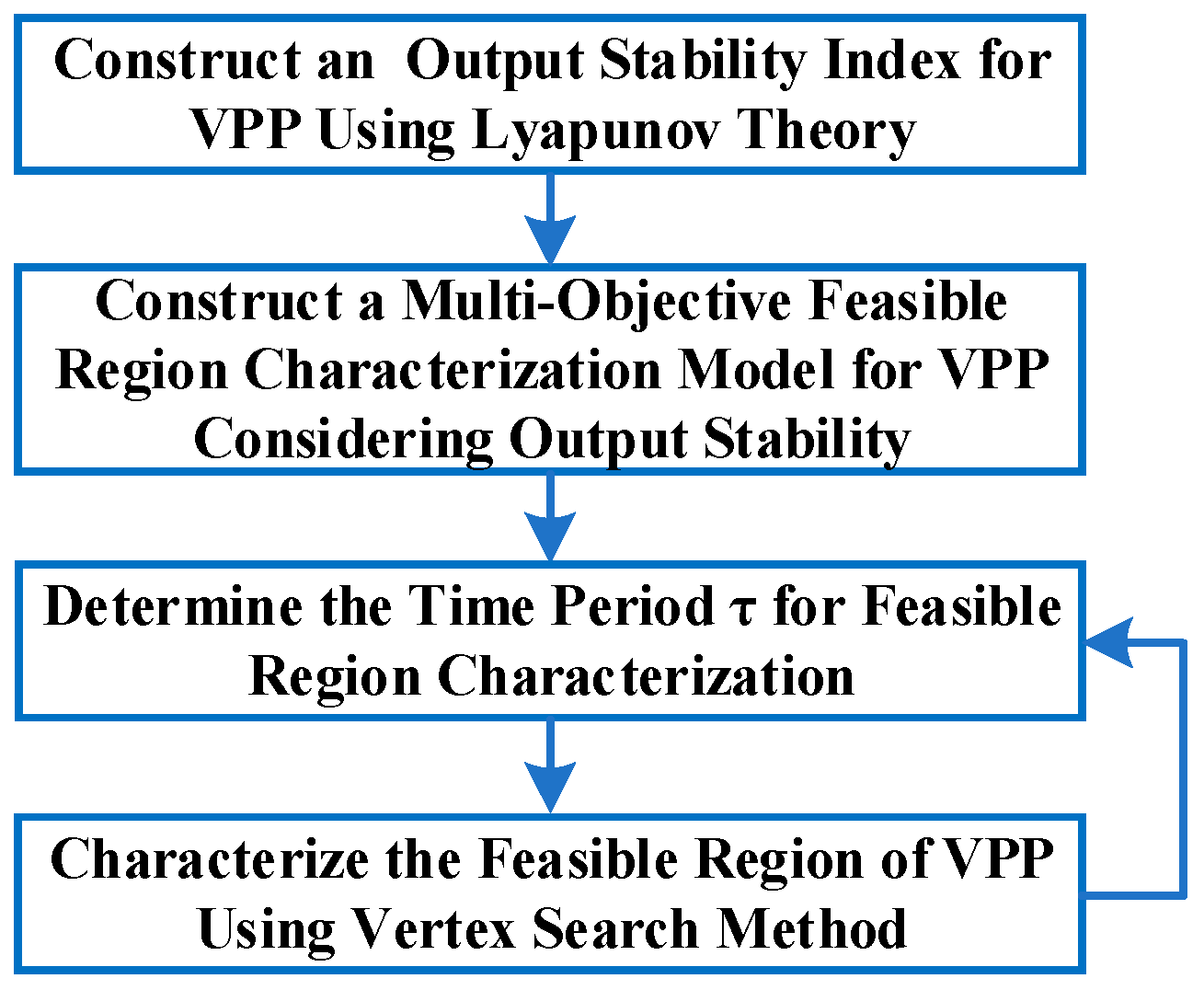
The brief process framework of the proposed method is shown in Figure 2. Firstly, this paper introduces Lyapunov theory to construct a VPP output stability index. Secondly, by integrating the VPP aggregation model, it develops a multi-objective feasibility region characterization model for VPPs considering output stability. Finally, it iteratively solves the temporal coupling feasibility regions of VPPs for different time periods, thereby obtaining the multi-objective time–domain coupled feasibility region of VPPs considering global stability.

The symbols and abbreviations used in this paper are listed in

Table 1. Nomenclature.

A. Acronyms:		$x_{ij}$	Reactance of the line
DER	Distributed energy resources	$c_{grid}^{pv}$$,l_{u,g}$$,c_t^{LD}$$c^{ES}$	Cost parameters of PV, MT, ES and LD
VPP	Virtual power plant	$\delta$, $h$	Convergence parameters of fixed-point search method
PV, MT, ES, LD	Photovoltaic, Microturbine, Energy-storage, Adjustable load	β, ρ	VPP expected return and stability index weight
ΩVPP	Approximate feasible region of VPP	${\mu }_t^{vpp}$	Unit Power Regulation Subsidy for VPP
PCC	Point of common coupling	$L_{pv}$$,L_{\mathrm{mt}}$$,L_{\mathrm{E}}$$,L_{\mathrm{L}}$	Numbers of PV, MT, ES and LD
B. Indices and Sets:		${\mathit{\mu }}_m^{\mathrm{T}}$	Direction parameters of vertex search method
p, g, e, l	Indices of PV, MT, ES and LD	D. Variables:
i, j	Indices of node	$P_{p,t}^{pv}$	PV output power
t	Indices of time	$P_{g,t}^{\mathrm{mt}}$	MT output power
m	Indices of iteration times of feasible region solution	$P_{e,t}^{\mathrm{ch}}$$,P_{e,t}^{\mathrm{dis}}$$,S_{\mathrm{OC},e,t}^{\mathrm{ES}}$	Energy storage charge power, discharge and state of charge
u, k	Indices of piecewise linear	$P_{l,t}^{\mathrm{L}}$$,S_{OL,l,t}$	LD power and reduction accumulation
C. Parameters:		$P_t^{\mathrm{PCC}}$	Interactive power of VPP at PCC
${\tilde{P}}_{p,t}^{pv}$$,{\alpha }_p$	Output expectation and confidence of PV	$P_{ij,t}^{\mathrm{LN}}$$,{\theta }_{i,t}$	Line power flow and the phase angle of the node
${\overline{P}}_{g,t}^{\mathrm{mt}}$$,∆P_{g,\max }^{\mathrm{mt}}$	Output and climbing upper limit of MT	${\delta }_t^{+}$$,{\delta }_t^{-}$	Continuous variables of absolute value linearization
$` {\overline{P}}_e^{\mathrm{ES}}$$,{\overline{S}}_{\mathrm{OC},e}^{\mathrm{ES}}$$,{\underset{\_}{S}}_{\mathrm{OC},e}^{\mathrm{ES}}$	1	$z_t^{+}$$,z_t^{-}$	Absolute value linearized 0-1 variables
${\overline{P}}_{l,t}^{\mathrm{L}}$$,{\underset{¯}{P}}_{l,t}^{\mathrm{L}}$$,{\tilde{S}}_{OL,l,t}$	Upper and lower limits of LD power and reduction accumulation	$∆P_t^{PCC}$	Regulating power provided by VPP
${\overline{P}}_{ij}^{\mathrm{LN}}$$,{\underset{¯}{P}}_{ij}^{\mathrm{LN}}$	Upper and lower limits of line power flow

.

2. The Feasible Region Characterization Model for VPPs

2.1. Establishment of VPP Model

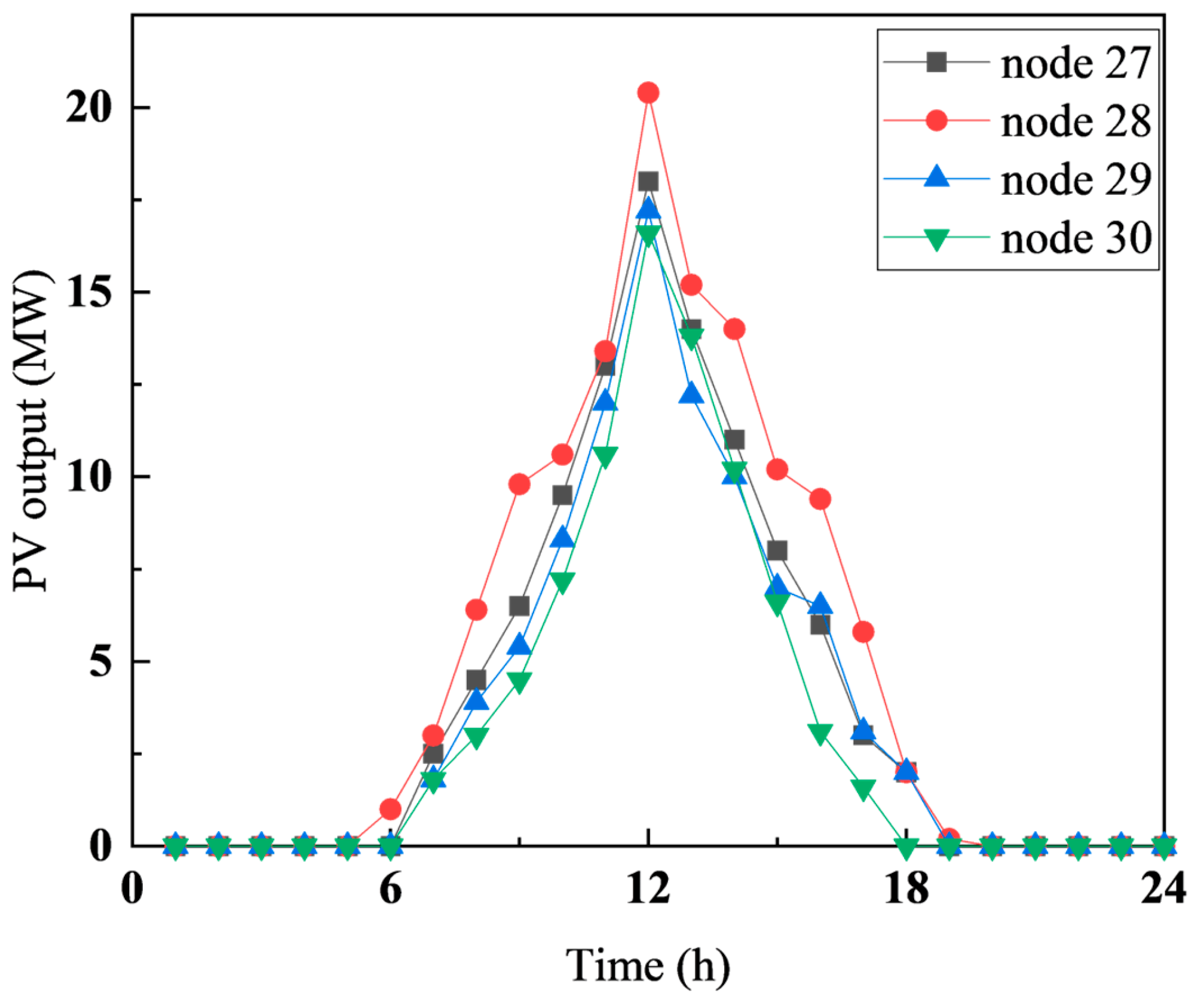
The aggregated resources within a VPP include DERs and flexible loads. Specifically, the DERs consist of distributed photovoltaic (PV) systems and distributed wind power, while the flexible loads include shiftable loads and distributed energy storage systems. The setting background for the feasible region model used in this paper involves the aggregation of large-scale flexible resources to participate in grid scheduling. Therefore, under the premise of establishing a reasonable model, a balance between detailed modeling and solution efficiency is sought. To achieve this, the study adopts the linearized power flow model proposed in Ref. [22].

2.1.1. DERs

• Distributed PV

Given the fluctuating nature of PV output, constraints involving random variables can be represented as chance constraints. This means that the constraints are maintained at a specific confidence level. The general form of a chance constraint is as follows:

$$P_{\mathrm{r}}\{P_{p,t}^{pv}\le {\tilde{P}}_{p,t}^{pv}\}\ge 1-{\alpha }_p$$

(1)

where $P_{\mathrm{r}}\{*\}$ is the probability that event $\{*\}$ holds true; $\widetilde{*}$ represents a random variable associated with $*$; ${\alpha }_{*}$ denotes the confidence level for the corresponding chance constraint.

The above chance constraints are transformed into deterministic constraints as:

$$P_{p,t}^{pv}\le Q_{\mathrm{uant}}({\alpha }_p| {\tilde{P}}_{p,t}^{pv})=C_{\mathrm{DF}{\tilde{P}}_{p,t}^{pv}}^{-1}({\alpha }_p)$$

(2)

where $Q_{\mathrm{uant}}({\alpha }_p|*)$ is the quantile; $C_{\mathrm{DF}{\tilde{P}}_{p,t}^{pv}}^{-1}(*)$ is the inverse function of $C_{\mathrm{DF}}$.

The specific form of Equation (2) can be calculated by giving the confidence level α into the corresponding $C_{\mathrm{DF}}$.

2.

Distributed gas turbine

The constraints of distributed gas turbines include output upper and lower bound constraints and ramp constraints.

$$0\le P_{g,t}^{\mathrm{mt}}\le {\overline{P}}_{g,t}^{\mathrm{mt}}$$

(3)

$$-∆P_{g,\max }^{\mathrm{mt}}\le P_{g,t}^{\mathrm{mt}}-P_{g,t-1}^{\mathrm{mt}}\le ∆P_{g,\max }^{\mathrm{mt}}$$

(4)

where $P_{g,t}^{\mathrm{mt}}$ is the active power output by $m{t}_g$ at time $t$; ${\overline{P}}_{g,t}^{\mathrm{mt}}$ is the upper limit of $m{t}_g$ output power at time $t$; $∆P_{g,\max }^{\mathrm{mt}}$ is the upper limit of $m{t}_g$ ramp power at time $t$.

3.

Distributed energy storage

The constraints of distributed energy storage include power constraints and state of charge (SOC) operation constraints [23,24,25]. The model is:

$$0\le P_{e,t}^{\mathrm{dis}}\le u_{e,t}^{\mathrm{ES}}{\overline{P}}_e^{\mathrm{ES}}$$

(5)

$$0\le \le (1-u_{e,t}^{\mathrm{ES}}){\overline{P}}_e^{\mathrm{ES}}$$

(6)

$$S_{\mathrm{OC},e,t+1}^{\mathrm{ES}}=S_{\mathrm{OC},e,t}^{\mathrm{ES}}+({\eta }_e^{\mathrm{ES}}{P}_{e,t}^{\mathrm{ch}}-P_{e,t}^{\mathrm{dis}}/{\eta }_e^{\mathrm{ES}})\mathsf{\Delta }t$$

(7)

$${\underset{\_}{S}}_{\mathrm{OC},e}^{\mathrm{ES}}\le S_{\mathrm{OC},e,t}^{\mathrm{ES}}\le {\overline{S}}_{\mathrm{OC},e}^{\mathrm{ES}}$$

(8)

$$S_{\mathrm{OC},e,0}^{\mathrm{ES}}=S_{\mathrm{OC},e,T}^{\mathrm{ES}}$$

(9)

where $P_{e,t}^{\mathrm{ch}}$ and $P_{e,t}^{\mathrm{dis}}$ are the charge and discharge power of energy storage e at time t, respectively; $u_{e,t}^{\mathrm{ES}}$ is the charge and discharge state of energy storage e at time t, 1 is discharge, 0 is charging; ${\overline{P}}_e^{\mathrm{E}}$ is the maximum charge and discharge power of energy storage e; $S_{\mathrm{OC},e,t}^{\mathrm{E}}$ is the state of charge of energy storage e at time t; ${\eta }_e^{\mathrm{E}}$ is the charge and discharge efficiency of energy storage e; ${\overline{S}}_{\mathrm{OC},e}^{\mathrm{E}}$ and ${\underset{\_}{S}}_{\mathrm{OC},e}^{\mathrm{E}}$ are the maximum and small state of charge of the energy storage e, respectively; $S_{\mathrm{OC},e,0}^{\mathrm{E}}$ is the initial state of charge of the energy storage e during the scheduling period; $S_{\mathrm{OC},e,T}^{\mathrm{E}}$ is the state of charge at the end of the energy storage e in the scheduling period.

4.

Flexible load

The VPP can interrupt the supply to flexible loads within acceptable limits, without affecting users’ comfort levels. This demonstrates the adjustable capability of flexible loads. The model for this is described as follows:

$${\underset{¯}{P}}_{l,t}^{\mathrm{L}}\le P_{l,t}^{\mathrm{L}}\le {\overline{P}}_{l,t}^{\mathrm{L}}$$

(10)

$$S_{OL,l,t+1}=S_{OL,l,t}+{\overline{P}}_{l,t}^{\mathrm{L}}-P_{l,t}^{\mathrm{L}}$$

(11)

$$0\le S_{OL,l,t}\le {\tilde{S}}_{OL,l,t}$$

(12)

$$S_{OL,l,0}=S_{OL,l,T}=0$$

(13)

where $P_{l,t}^{\mathrm{L}}$ is the actual power of the adjustable load l in the VPP; ${\overline{P}}_{l,t}^{\mathrm{L}}$ and ${\underset{¯}{P}}_{l,t}^{\mathrm{L}}$ are the upper and lower limits of the adjustable load power in the VPP, ${\overline{P}}_{l,t}^{\mathrm{L}}=1.2P_{l,t}^{\mathrm{L},\mathrm{real}},{\underset{¯}{P}}_{l,t}^{\mathrm{L}}=0.5P_{l,t}^{\mathrm{L},\mathrm{real}}$, where $P_{l,t}^{\mathrm{L},\mathrm{real}}$ is the actual power demand of the load; $S_{OL,l,t}$ represents the accumulated electricity that does not meet the load demand.

2.1.2. Network Constraint

The network constraints are represented as follows:

$$P_{ij,t}^{\mathrm{LN}}=({\theta }_{i,t}-{\theta }_{j,t})/x_{ij}$$

(14)

$$\sum _{p=1}^{L_{pv}}{P}_{j,p,t}^{pv}+\sum _{g=1}^{L_{\mathrm{mt}}}{P}_{j,g,t}^{\mathrm{mt}}-\sum _{l=1}^{L_{\mathrm{L}}}{P}_{j,l,t}^{\mathrm{L}}+\sum _{e=1}^{L_{\mathrm{E}}}(P_{j,e,t}^{\mathrm{dis}}-P_{j,e,t}^{\mathrm{ch}})-P_t^{\mathrm{PCC}}=\sum _{ji\in {\mathsf{\Lambda }}_j^{\mathrm{LN}}}{P}_{ji,t}^{\mathrm{LN}}$$

(15)

$$-2pi\le {\theta }_{i,t}\le 2pi$$

(16)

$${\underset{¯}{P}}_{ij}^{\mathrm{LN}}\le P_{ij,t}^{\mathrm{LN}}\le {\overline{P}}_{ij}^{\mathrm{LN}}$$

(17)

where $P_{ij,t}^{\mathrm{LN}}$ is the active power of line ij at time t; $x_{ij}$ is the reactance of line ij; ${\theta }_{i,t}$ is the phase angle of node i at time t; $P_t^{\mathrm{PCC}}$ is the external active power output of VPP at time t; ${\overline{P}}_{ij}^{\mathrm{LN}}$, and ${\underset{¯}{P}}_{ij}^{\mathrm{LN}}$ are the upper and lower limits of active power flow of line ij.

2.1.3. Return Constraint

Given that the stability of a VPP alliance relies on objective revenues to sustain itself, profitability is a necessary condition for the formation of a feasible region for the VPP. To address this, this paper considers the dispatch costs and revenues of various resources within the VPP and constructs revenue chance constraints for the VPP as follows:

$${\mu }_t^{vpp}\left|∆P_t^{PPC}\right|-{\displaystyle \sum _t^T\left\{\sum _{p=1}^{L_{pv}}{C}_{p,t}^{pv}+\sum _{g=1}^{L_{\mathrm{mt}}}{C}_{g,t}^{mt}+\sum _{l=1}^{L_{\mathrm{L}}}{C}_{l,t}^{LD}+\sum _{e=1}^{L_{\mathrm{E}}}{C}_{e,t}^{ES}\right\}}\ge \beta$$

(18)

where $\left|∆P_t^{PPC}\right|$ represents the difference between the VPP and the original operating point. Considering that there is a nonlinear term $\left|∆P_t^{PPC}\right|$ in the revenue opportunity constraint of the VPP, this paper completely linearizes $\left|∆P_t^{PPC}\right|$ by mathematical method. The linearized revenue opportunity constraint is as follows:

$$\left\{\begin{array}{l}{\mu }_t^{vpp}({\delta }_t^{+}+{\delta }_t^{-})-{\displaystyle \sum _t^T\left\{\sum _{p=1}^{L_{pv}}{C}_{p,t}^{pv}+\sum _{g=1}^{L_{\mathrm{mt}}}{C}_{g,t}^{mt}+\sum _{l=1}^{L_{\mathrm{L}}}{C}_{l,t}^{LD}+\sum _{e=1}^{L_{\mathrm{E}}}{C}_{e,t}^{ES}\right\}}\ge \beta \\ {\delta }_t^{+}\ge 0,{\delta }_t^{+}\le 0+M\times (1-z_t^{+})\\ {\delta }_t^{+}\ge ∆P_t^{PCC},{\delta }_t^{+}\le ∆P_t^{PCC}+M\times (1-z_t^{+})\\ {\delta }_t^{-}\ge 0,{\delta }_t^{-}\le 0+M\times (1-z_t^{-})\\ {\delta }_t^{-}\ge -∆P_t^{PCC},{\delta }_t^{-}\le -∆P_t^{PCC}+M\times (1-z_t^{-})\\ z_t^{+}+z_t^{-}\ge 1\end{array}\right.$$

(19)

where ${\mu }_t^{vpp}$ represents the adjustment power compensation of VPP; ${\delta }_t^{+}$ and ${\delta }_t^{-}$ are linear variables representing absolute values; $M$ is a maximal number; $z_t^{+}$ and $z_t^{-}$ are Boolean variables; $C_{p,t}^{pv}$ represents the adjustment cost of photovoltaic in VPP; $C_{g,t}^{mt}$ represents the regulation cost of micro gas turbine in VPP; $C_{l,t}^{LD}$ represents the adjustment cost of flexible load in VPP; $\beta$ is the adjusted expected return of VPP.

1.

Regulation cost of PV

$$C_{p,t}^{pv}=c_{grid}^{pv}∆P_{p,t}^{pv}$$

(20)

where $c_{grid}^{pv}$ is the photovoltaic on-grid price; $∆P_{p,t}^{pv}$ represents the output offset of PV units in the process of VPP feasible region boundary characterization.

2.

Regulation cost of micro gas turbine

In this paper, the secondary operation cost function of the micro gas turbine is piecewise linearized, as shown below.

$$C_{g,t}^{mt}={\displaystyle \sum _{u=1}^n(}{l}_{u,g}∆P_{u,g,t}^{mt})$$

(21)

where $l_{u,g}$ represents the piecewise linearization slope of the quadratic cost function of the micro gas turbine; $∆P_{u,g,t}^{mt}$ represents the offset of the output of the gas turbine in the linearization stage u.

3.

Regulation cost of flexible load

$$C_{l,t}^{LD}=c_t^{LD}∆P_{l,t}^{\mathrm{L}}$$

(22)

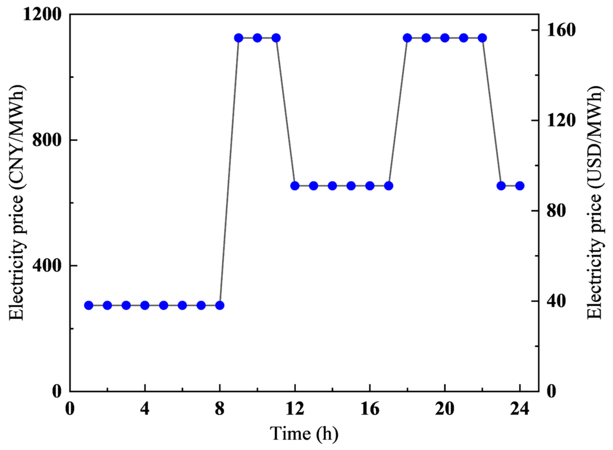
where $c_t^{LD}$ is the electricity price of the flexible load at time t; $∆P_{l,t}^{\mathrm{L}}$ represents the offset between the flexible load l and the original power demand at time t.

4.

Regulation cost of energy storage

$$C_{e,t}^{ES}=c^{ES}(∆P_{e,t}^{\mathrm{dis}}+∆P_{e,t}^{\mathrm{ch}})$$

(23)

where $c^{ES}$ is the operating cost of energy storage unit; $∆P_{e,t}^{\mathrm{ch}}$ and $∆P_{e,t}^{\mathrm{dis}}$ represent the offset between the energy storage charging and discharging power and the original operating point.

2.2. Virtual-Power-Plant-Feasible Region Search Method

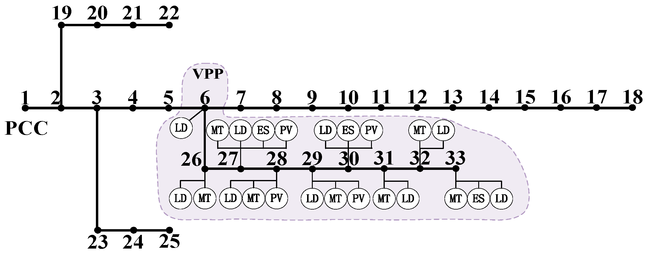
Given that all constraints within the VPP model are linear constraints, the facets of the high-dimensional polytope characterized by the VPP model are all planes. Therefore, the projection of this polytope into lower dimensions results in a polygon with a finite number of edges. The vertex search method’s basic approach involves solving a sequence of optimization problems that have varying objective functions. This process is designed to systematically identify each vertex of the feasible region. Once all vertices are obtained, the next step is to compute the convex hull from these vertices, which ultimately delineates the feasible region as a polygon. In the subsequent sections, we will first define the optimization problems and the conditions under which the algorithm terminates. Finally, we will provide a detailed explanation of the vertex search method process.

1.

Optimization method problem

Firstly, the objective function of the feasible region vertex search is determined to be:

$$\underset{p}{\max } {\mathit{\mu }}_m^{\mathrm{T}}{\mathit{p}}_{m,t},{\mathit{p}}_{m,t}\in {\Omega }_{\mathrm{VPP}}$$

(24)

where ${\mu }_m^{\mathrm{T}}=\left[\begin{array}{c}{\mu }_{P(t),m},{\mu }_{P(t-1),m}\end{array}\right]$ is the unit direction vector for searching the new vertex; ${\mathit{p}}_{m,t}=\left[\begin{array}{c}{P}_t^{PCC},P_{t-1}^{PCC}\end{array}\right]$ is the variable representing the overall external feasible region of the virtual power plant, which is the point in the feasible region ${\Omega }_{\mathrm{VPP}}$.

The optimal solution of each optimization problem under different ${\mu }_m^{\mathrm{T}}$ is represented by the coordination variable ${\mathit{p}}_{m,t}$, which corresponds to a vertex of the feasible region.

2.

Stopping condition

The polygon represented by the neighborhood feasible region boundary is a collection of vertices and edges. Among the different characteristics between new vertices and original vertices, relative displacement is one of the most intuitive and effective measures. Therefore, the termination condition is set as the relative displacement of a new vertex from its corresponding original line being less than a specific value $\delta$. Let the relative displacement be $h_j$, that is:

$$h_j={\mathit{\mu }}_m^{\mathrm{T}}(z_{2,t}-z_{0,t})/\left|\right|{\mathit{\mu }}_m|{|}_2\le \delta$$

(25)

where $z_{0,t}$ is the new vertex generated at time t; $z_{2,t}$ is the vertex on the clockwise side of the generated new vertex; $\left|\right|{\mathit{\mu }}_m|{|}_2$ is the two norm of the search direction vector; $\delta$ is the set termination condition.

3.

Algorithm procedure

The vertex search method transforms the problem of constructing the feasibility region of a VPP into an optimization problem of the VPP’s external power output. Therefore, the VPP’s output boundaries can be iteratively solved using the GUROBI solver. The process of solving the time-neighbor-feasible region based on the vertex search method is shown in Figure 3:

Step 1: The time-neighborhood-feasible region of the solution time t is determined, and the direction vector set ${\mathit{\mu }}_1^{\mathrm{T}}\in U_{1,t}=[(1,0),(0,-1),(-1,0),(0,1)]$ and the vertex set $Z_{1,t}=\varnothing$ are initialized.

Step 2: ${\mathit{p}}_{m,t}$ belonging to different ${\mathit{\mu }}_m^{\mathrm{T}}$ is obtained in turn and stored in the vertex set ${\mathit{z}}_{2,t}$.

Step 3: The unit outer normal vector between all adjacent vertices is calculated as the direction vector of the next round of search, and the direction vector set $U_{2,t}$ is updated.

Step 4: The $h_j$ corresponding to each vertex is calculated. If the $h_j$ corresponding to a vertex is less than the set threshold $\delta$, the outer normal vector search link determined by the vertex and the adjacent vertex is stopped. If it is greater than the set threshold $\delta$, steps 2–4 are repeated until all vertices $h_j$ meet the termination condition.

Step 4: By solving the convex hull of each vertex, the time–domain coupling feasible region of t − 1 time and t time is obtained.

3. Lyapunov-Based VPP Global Stability Problem Transformation

In the process of characterizing the boundary of the feasible region for the VPP using the vertex search method, constraints such as those expressed in Equations (7), (9), (11), and (13) introduce time–coupling effects. Searching for the boundary at a single time point can lead to cascading changes in power output at other time points, resulting in a lack of global stability in the VPP’s power output. Therefore, it is necessary to perform wide-area temporal decoupling of the VPP to ensure global stability during the feasible region boundary search process. This paper, referencing literature [26], employs a Lyapunov function to represent the stability of VPP power output, with the specific approach detailed below.

3.1. Construct Virtual Queue

This paper constructs virtual queues for VPP output based on the principles of Lyapunov stability analysis. These virtual queues are used to analyze the stability of the VPP, specifically by modeling the global output within the VPP.

Firstly, a virtual queue $Q_t$ is constructed for the VPP to reflect the cumulative offset of the VPP relative to the original operating point in the process of feasible region boundary characterization, that is:

$$Q_{t+1}=Q_t+{\widehat{P}}_t^{PCC}-P_t^{PCC}$$

(26)

The concept of virtual queues can be used to describe the stability of the wide-time-domain output in the VPP as the net flow value of virtual queues being zero over a certain period. This can be equivalently framed as a stability problem of the virtual queues.

3.2. Multi-Objective Problem Transformation Based on Lyapunov Function

To address the stability issues of virtual queues, this paper constructs a Lyapunov function that characterizes the congestion level of these virtual queues. This approach enables the modeling and solving of the virtual queue stability problem, leading to the development of a robust stability model for VPP [26].

Firstly, the Lyapunov function $H_t$ is constructed as

$$H_t={\displaystyle \frac{Q_t^2}{2}}$$

(27)

From the above discussion, it can be seen that when $H_t$ is small, all virtual queues experience low congestion levels, leading to better stability of the virtual queues. Conversely, when $H_t$ is large, at least one virtual queue will have a high congestion level, resulting in poor stability of the virtual queues. Therefore, the stability problem of VPP output can be relaxed into a problem of minimizing $H_t$.

However, Equation (27) contains squared terms of the variables, transforming the original optimization problem into a Mixed-Integer Quadratically Constrained Program (MIQCP). This significantly increases the computational burden on the solver. To simplify the computation, this paper employs the principle of piecewise linearization to convert Equation (27) into piecewise lower bounds. The detailed process is described below.

$$Q_t^{sq}\ge {\mathrm{S}}_k^{\mathrm{lopes}}{Q}_t+{\mathrm{I}}_k^{\mathrm{ntercept}}$$

(28)

$$H_t^{sq}={\displaystyle \frac{Q_t^{sq}}{2}}$$

(29)

where $Q_t^{sq}$ is a square linear variable, which represents the value of $Q_t^2$ after piecewise linearization; ${\mathrm{S}}_k^{\mathrm{lopes}}$ denotes the slope of the kth segment; ${\mathrm{I}}_k^{\mathrm{ntercept}}$ denotes the intercept of paragraph k; $H_t^{sq}$ is the piecewise linearized Lyapunov function. Through Equations (29) and (30), the original problem is transformed from finding the minimum A to taking the lower boundary of B, and the original MIQCP is transformed into a MILP problem, which greatly improves the efficiency of problem solving.

To ensure the stability of virtual queues over the entire time period, while also considering the vertex search objective function represented by Equation (20), we refer to the L-DPP function from reference [27]. The original problem is transformed into a vertex characterization problem that considers the overall stability of virtual queues in the VPP. The detailed formulation is provided below.

$$\underset{x}{\min }-{\mathit{\mu }}_m^{\mathrm{T}}{\mathit{p}}_{m,t}+\rho {\displaystyle \frac{1}{T}}{\displaystyle \sum _t^T{H}_{m,t}^{sq}}$$

(30)

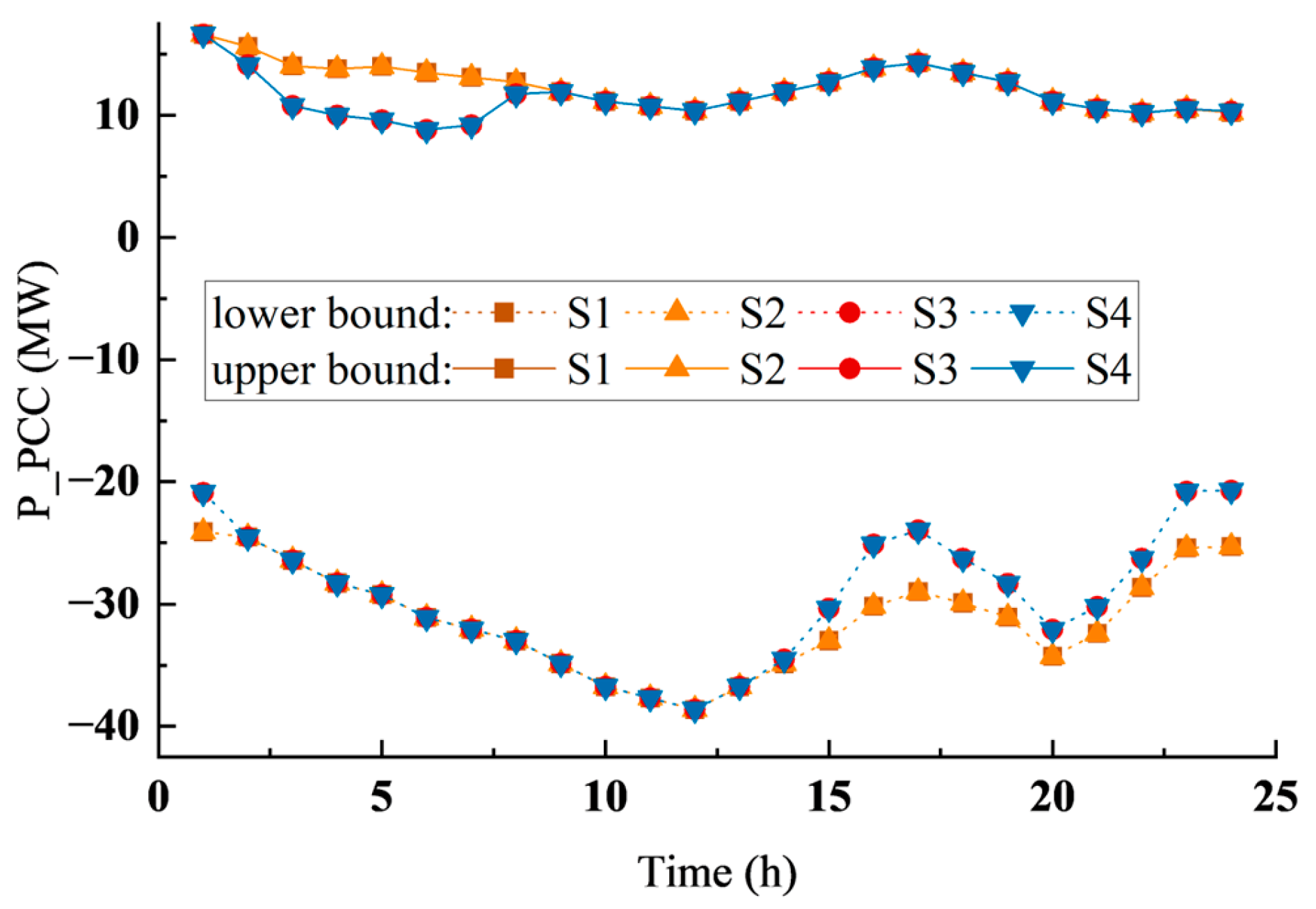
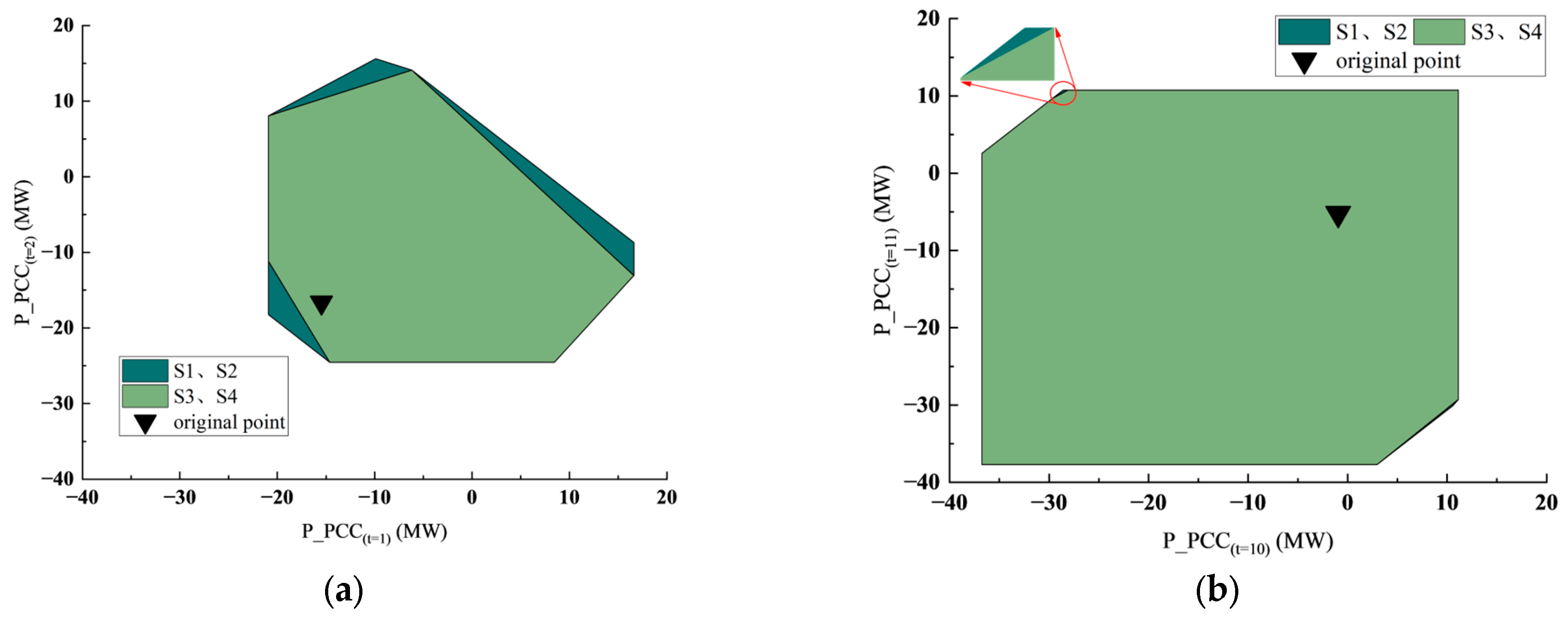
By combining constraints (1)–(17), (19)–(23), (26), and (28)–(30), we formulate the multi-objective time-neighborhood-feasible region construction method proposed in this paper, which considers the full-time sequential coupling stability of the VPP.

4. Results Analysis

In order to verify the feasibility of the algorithm in this paper, the node {6, 26–33} in the IEEE-33 node system is selected as the topology of the VPP, and the VPP is regarded as the access node 6. All test cases are based on MATLAB-2023 platform, AMD R9-7845 HX CPU and commercial solver GUROBI 12.0.

4.1. Example Scenario

4.1.1. Resource and Scene Settings

1.

Resource settings

The aggregated model of the VPP constructed in this paper includes four distributed PV units (Access nodes 27–30), seven distributed gas turbine units (Access nodes 26–29 and 31–33), three energy storage units, and nine adjustable load units (Access nodes 6,26–33), as specifically illustrated in Figure 4. A VPP achieves revenue by aggregating distributed resources and modifying their operating profiles to provide regulation services to the grid illustrated in the figure.

2.

Scenarios setting

In order to verify the effectiveness of the proposed method, this paper compares and analyzes the following four scenarios:

S1: The revenue constraint of the VPP and the wide time domain output stability of the VPP are not considered.

S2: Considering the revenue constraint of the VPP, the wide time domain output stability of the VPP is not considered.

S3: Without considering the revenue constraint of the VPP, the wide time domain output stability of the VPP is considered.

S4: At the same time, the revenue constraint of the VPP and the stability of the VPP wide-time domain output are considered.

4.1.2. Unit Parameter Setting

The access point of distributed energy storage is {27,30,33}, and the access point of the distributed gas turbine is {26,27,28,29,31,32,33}. The specific equipment and cost parameters are shown in the following

Table 2. Distributed energy storage and gas turbine-related parameters.

ES	Data	MT	Data
node	{27,30,33}	node	{26,27,28,29,31,32,33}
${\overline{P}}_e^{\mathrm{E}}$	{6,4,5} (MW)	${\overline{P}}_{g,t}^{\mathrm{mt}}$	{20,20,24,24,20,20,20} (MW)
${\eta }_e^{\mathrm{E}}$	{0.95,0.95,0.95}	$∆P_{g,\max }^{\mathrm{mt}}$	{6,6,6,4,5,5,5} (MW/h)
${\overline{S}}_{\mathrm{OC},e}^{\mathrm{E}}$	{10.8,7.2,9} (MWh)	$l_{u,g}$	360/480/580/650 (CNY/MWh)
${\underset{\_}{S}}_{\mathrm{OC},e}^{\mathrm{E}}$	{1.2,0.8,1} (MWh)	/	/
$c^{ES}$	210 (CNY/MWh)	/	/

. The table sets the parameters for ES and MT resources, including the ES charge/discharge power limits ${\overline{P}}_e^{\mathrm{E}}$, ES charge/discharge efficiency ${\eta }_e^{\mathrm{E}}$, ES energy capacity limits ${\overline{S}}_{\mathrm{OC},e}^{\mathrm{E}}$ and ${\underset{\_}{S}}_{\mathrm{OC},e}^{\mathrm{E}}$, ES operational cost $c^{ES}$, MT generation power limit ${\overline{P}}_{g,t}^{\mathrm{mt}}$, MT ramp rate limit $∆P_{g,\max }^{\mathrm{mt}}$, and MT generation cost parameters $l_{u,g}$.

The output prediction data of distributed photovoltaic are shown in Figure 5 below, and the on-grid price $c_{grid}^{pv}$ is 391 CNY/MWh (54.38 USD/MWh).

The original load demand of the distributed adjustable load refers to the standard example data of the IEEE 33 node distribution network. The electricity price $c_t^{LD}$ of the flexible load in this paper refers to the time-of-use electricity price of September 2024 in Jiangsu Province, China, as shown in Figure 6. The grid guides the electricity consumption profiles of users by setting time-of-use pricing. Similarly, a VPP can also reduce electricity costs and generate revenue by adjusting the consumption profiles of flexible loads.

4.2. Analysis of Feasible Region Characterization Results

Due to the significant influence of global stability indicator weights on the time- neighborhood-feasible region considering full-time sequential coupling stability of VPPs constructed in this paper, this section first calculates the output boundaries and feasible regions under different VPP stability indicator weights. By analyzing the feasible regions under various weights, appropriate weight values are selected. Secondly, based on the selected weight values, the feasible regions for the four scenarios set in Section 4.1.1 are characterized, and the impacts of economic constraints and stability on the feasible region characterization are analyzed. Finally, based on the constructed economic constraints, the feasible regions under different economic parameters are characterized to study their impact on the feasible region boundaries.

4.2.1. Weight Sensitivity Analysis of VPP Stability Index

Due to the significant impact of the global stability indicator weights on the characterization of VPP-feasible region boundaries, this subsection selects five weight scenarios: ρ = 0.1, 0.5, 1, 10, 100 for VPP-feasible region characterization and analysis. The resulting VPP output boundary characterization is shown in Figure 7.

Figure 7 illustrates the upper and lower boundaries of VPP output at each time point under different indicator weights. It can be observed that as the indicator weight increases, the decoupling degree between the time neighborhood and time global solutions becomes higher. Consequently, the VPP has less flexibility to adjust its output across different time periods. For instance, when ρ = 100, during the 20:00 time slot, the VPP has less than 5 MW of adjustment capability. To better understand the impact of ρ on the VPP’s adjustment capability, this subsection also characterizes the time-neighborhood-feasible regions for the periods 1:00–2:00 and 10:00–11:00 under different indicator weights. The characterization results are shown in Figure 8.

Figure 8 characterizes the time-neighborhood-feasible regions for the periods 1:00–2:00 and 10:00–11:00 under different indicator weights ρ. The time-neighborhood-feasible region can be viewed as the relationship between adjacent time slices in the VPP, representing the relationship between the output at the previous time slice and the next time slice. Once the specific output of the previous time slice is determined, the upper and lower limits of the VPP’s output at the current time slice can be determined, i.e., the ramping parameters.

From Figure 8a, it can be observed that when ρ exceeds 10, for the period 1:00–2:00, the VPP can no longer obtain additional regulation capacity from other time periods, and the feasible region is compressed into a single line. The VPP loses its multi-period adjustment capability, meaning that the output is determined. From Figure 8b, it can be seen that when ρ is less than or equal to 1, the impact of ρ on the VPP’s feasible region is relatively small. Changing ρ from 0.1 to 1 results in only a 0.06% reduction in the feasibility region area. However, when ρ exceeds 10, the temporal coupling feasibility region of the VPP is compressed into a line segment defined by the endpoints {P_t=10 = −16.91 MW, P_t=11 = 10.73 MW} and {P_t=10 = 11.13 MW, P_t=11 = −17.31 MW}, significantly limiting the adjustment capability at the vertices.

In summary, based on the calculation and analysis results, it can be seen that the value of the weight ρ significantly affects the feasible region of the VPP. When ρ is set to a value of 10 or higher, the VPP cannot obtain adjustment potential from other time domains, and its feasible region is compressed to an extremely small area, severely limiting the flexibility of the VPP. To balance flexibility and stability, this paper selects ρ = 1 and conducts subsequent case studies based on this value change.

4.2.2. Feasibility Analysis of Scheme

Based on the data and scene Section 4.1, this paper measures the VPP output boundary and time-neighborhood-feasible region (β = 0 and ρ = 1) under the comparison scenarios of S1, S2, S3, and S4, and then analyzes the economic constraints and stability indicators. The impact of the results of the VPP feasible region characterization is shown in Figure 9 and Figure 10.

Figure 9 characterizes the output boundaries of the VPP in different scenarios. As shown, due to the decoupling effect of the global stability indicator, the VPP’s output boundaries are significantly affected. The VPP with global stability indicators has a smaller output range during the periods 1:00–8:00 and 15:00–24:00 (For example, at 6:00, the upper limit of VPP output decreases from 13.48 MW to 8.81 MW, and at 17:00, the lower limit of VPP output increases from −29 MW to −23.95 MW), which better aligns with real-world operational scenarios. Regarding whether to consider VPP revenue constraints, the output boundaries in scenarios S1 and S2, which do not consider revenue constraints, almost overlap. Similarly, the output boundaries in scenarios S3 and S4, which do consider revenue constraints, also almost overlap. This is because, in the context of this study where the VPP provides regulation services to the grid, the unit power regulation subsidy provided by the grid is set at 2000 CNY/MWh, which exceeds the unit regulation cost of the VPP’s aggregated resources, ensuring that the VPP can always achieve positive revenue from providing regulation services.

Figure 10 characterizes the time-neighborhood-feasible regions of the VPP for the periods 1:00–2:00 and 10:00–11:00 under different comparison scenarios. From this figure, it can be analyzed that during the periods 1:00–2:00 and 10:00–11:00, the feasible regions in scenarios S1 and S2 almost overlap, as do those in scenarios S3 and S4. This is because the subsidy parameters for the VPP are greater than the cost parameters, ensuring that the VPP can always achieve positive revenue from providing regulation services, consistent with the analysis results of Figure 9. Additionally, regarding whether to consider the global output stability index, during the 1:00–2:00 period, after considering the global output stability index, the upper and lower bounds of the VPP’s adjustable power region based on the original nodes are reduced. From the perspective of the feasible region area, this reduction is approximately 8.56%. In contrast, during the 10:00–11:00 period, the VPP’s adjustable power region only experiences a minor reduction in the power nodes {P_t=10 = 28.58 MW, P_t=11 = 10.73 MW} and {P_t=10 = 10.56 MW, P_t=11 = −30.08 MW}.

4.2.3. Sensitivity Analysis of VPP Economic Constraints

From the analysis in the previous section, it can be concluded that when β = 0, whether or not to consider VPP revenue constraints has a minimal impact on the time-neighborhood-feasible region of the VPP. Therefore, to study the impact of the VPP operator’s expected revenue on the feasible region, this section employs sensitivity analysis by varying the parameter β to characterize the economic feasible region of the VPP, as shown in Figure 11.

During the calculation process, when β = 0/5 × 10⁴/1 × 10⁵ CNY (0/6954.2/13,908.4 USD), the economic neighborhood feasible regions of the VPP overlap. The reason for this phenomenon is that although the VPP’s regulation subsidy revenue has a linear relationship with the regulation power, the VPP can adjust the distribution of internal electric energy and modify its generation and consumption plans to reduce overall costs. Therefore, in Figure 11, only the economic neighborhood feasible regions for β = 1 × 10⁵/1.5 × 10⁵ CNY (13,908.4/20,862.6 USD) are depicted.

When β = 1.5 × 10⁵ CNY (20,862.6 USD), during the 1:00–2:00 period, most of the VPP’s economically feasible region appears in the outward power discharge area (i.e., the light blue area). This means that to achieve additional revenue above an expected revenue of 1.5 × 10⁵ CNY (20,862.6 USD), the VPP must regulate its outward output to {P_t=1 ≤ 7.27 MW∩P_t=2 ≥ −1.93 MW, P_t∈${\Omega }_{\mathrm{VPP}}$} to realize corresponding extra revenue. In contrast, during the 10:00–11:00 period, the VPP’s economically feasible region appears in the deep consumption power area (i.e., the light blue area). This indicates that to achieve additional revenue above an expected revenue of 1.5 × 10⁵ CNY (20,862.6 USD), the VPP must regulate its outward output to {P_t=10 ≥ −23.42 MW∩P_t=11 ≤ −29.47 MW, P_t∈${\Omega }_{\mathrm{VPP}}$}. The feasible regions for both periods show significant deviations from the original operating points. This is because the model proposed in this study calculates adjustment revenue based on the regulation provided by the VPP relative to its original operating power. The greater the deviation from the original operating point is, the higher is the adjustment revenue. During the 10:00–11:00 period, when electricity prices are highest, the VPP needs to provide more regulation to achieve excess revenue, resulting in a smaller feasible region and larger deviation from the original operating point.

Through the aforementioned sensitivity analysis method targeting economic constraints, VPP operators can obtain the economically feasible region of the VPP based on their own operational conditions and expected revenues. This information can then be reported to the grid dispatch department for use in real-time grid scheduling and regulation.

5. Conclusions

In response to the limitations of existing methods that do not consider the stability of wide-area time–period output, this paper proposes a multi-objective feasible region search problem that incorporates Lyapunov stability indicators. By constructing a method for building a multi-objective time–domain coupled feasible region for VPPs with global stability considerations, we characterize the feasible output region of neighboring time periods for VPPs while ensuring the stability of wide-area time–period outputs.

The multi-objective time–domain coupled feasible region construction method for VPPs with global stability considerations proposed in this paper has the following characteristics:

• The proposed method can accurately characterize the neighborhood output feasible region of VPPs. Based on this neighborhood feasible region, VPP operators can precisely assess the output boundaries and ramping boundaries of the VPP.
• The proposed method introduces a global output stability indicator for VPPs. Through multi-objective optimization, it achieves varying degrees of decoupling between neighborhood and wide-area considerations. When characterizing the neighborhood feasible region of VPPs, this approach reduces the deviation in wide-area output, thereby ensuring global stability.
• The proposed method introduces VPP revenue constraints, enabling VPP operators to effectively assess the potential revenue from regulation commands by controlling these constraints. This approach helps VPP operators make informed decisions that balance economic benefits and operational stability.

In summary, the proposed method provides a methodology for VPPs to assess the output boundaries and ramping parameters of aggregated resources. By employing the neighborhood feasible region characterization method provided in this paper, it is possible to accurately characterize the output boundaries and ramping boundaries of VPPs while ensuring the stability of wide-area outputs. This approach meets the practical needs of evaluating VPP regulation capabilities, encourages VPP operators to actively participate in the regulation market, and promotes long-term sustainable operations.

While addressing key issues in the field of VPP regulation capability assessment, this paper also has limitations. It primarily uses conventional vertex search methods to characterize the VPP’s feasible region and does not employ fixed-point methods or AC region approximation to optimize the efficiency and accuracy of characterizing the feasible region for massive resource aggregation. Additionally, this paper ignores the impact of source-load uncertainty on the boundaries of the VPP’s feasible region.

Future research should focus on designing more efficient and accurate algorithms for characterizing the feasible region, such as improving vertex search methods using fixed-point methods or combining convex polyhedron approximation with mathematical programming to accommodate massive heterogeneous distributed resources. Additionally, considering the risks of output and command response uncertainties in the process of characterizing the VPP’s feasible region will also be a key focus of future research.

References

1. Li, J.; Huang, Y.; Dou, X.; Wang, S.; Chu, T. Optimal Energy Storage Configuration for Primary Frequency Regulation Performance Considering State of Charge Partitioning. IEEE Trans. Sustain. Energy 2025, 1–9, early access. [Google Scholar] [CrossRef]
2. Qin, Y.; Rao, Y.; Xu, Z.; Lin, X.; Cui, K.; Du, J.; Ouyang, M. Toward Flexibility of User Side in China: Virtual Power Plant (VPP) and Vehicle-to-Grid (V2G) Interaction. eTransportation 2023, 18, 100291. [Google Scholar] [CrossRef]
3. Kong, X.; Lu, W.; Wu, J.; Wang, C.; Zhao, X.; Hu, W.; Shen, Y. Real-Time Pricing Method for VPP Demand Response Based on PER-DDPG Algorithm. Energy 2023, 271, 127036. [Google Scholar] [CrossRef]
4. Elgamal, A.H.; Shahrestani, M.; Vahdati, M. Simultaneous Sizing and Energy Management of Multi-Energy Virtual Power Plants Operating in Regulated Energy Markets. Int. J. Electr. Power Energy Syst. 2024, 161, 110171. [Google Scholar] [CrossRef]
5. Li, Q.; Wei, F.; Zhou, Y.; Li, J.; Zhou, G.; Wang, Z.; Liu, J.; Yan, P.; Yu, D. A Scheduling Framework for VPP Considering Multiple Uncertainties and Flexible Resources. Energy 2023, 282, 128385. [Google Scholar] [CrossRef]
6. Li, D.; Wang, M.; Shen, Y.; Li, F.; Lin, S.; Zhou, B. Low-Carbon Operation Strategy of Virtual Power Plant Considering Progressive Demand Response. Int. J. Electr. Power Energy Syst. 2024, 161, 110176. [Google Scholar] [CrossRef]
7. Zhou, Y.; Essayeh, C.; Morstyn, T. A Novel Surrogate Polytope Method for Day-Ahead Virtual Power Plant Scheduling with Joint Probabilistic Constraints. Electr. Power Syst. Res. 2024, 234, 110623. [Google Scholar] [CrossRef]
8. Ren, J.; Zeng, Y.; Qin, C.; Li, B.; Wang, Z.; Yuan, Q.; Zhai, H.; Li, P. Characterization and Application of Flexible Operation Region of Virtual Power Plant. Appl. Energy 2024, 371, 123733. [Google Scholar] [CrossRef]
9. Wang, J.; Xing, X.; Fu, Z.; Hai, C.; Liu, H.; Wang, Q. Feasible Region Analysis of PV Hosting Capacity in Active Distribution Networks via a Two-Stage Optimization Approach. Electr. Power Syst. Res. 2025, 242, 111446. [Google Scholar] [CrossRef]
10. Cui, X.; Liu, S.; Ruan, G.; Wang, Y. Data-Driven Aggregation of Thermal Dynamics within Building Virtual Power Plants. Appl. Energy 2024, 353, 122126. [Google Scholar] [CrossRef]
11. Meng, W.; Song, D.; Huang, L.; Chen, X.; Yang, J.; Dong, M.; Talaat, M.; Elkholy, M.H. Distributed Energy Management of Electric Vehicle Charging Stations Based on Hierarchical Pricing Mechanism and Aggregate Feasible Regions. Energy 2024, 291, 130332. [Google Scholar] [CrossRef]
12. Liu, X.; Lin, X.; Qiu, H.; Li, Y.; Huang, T. Optimal Aggregation and Disaggregation for Coordinated Operation of Virtual Power Plant with Distribution Network Operator. Appl. Energy 2024, 376, 124142. [Google Scholar] [CrossRef]
13. Saad Suliman, M.; Farzaneh, H. Data-Driven Modeling of the Aggregator-Based Price-Maker Virtual Power Plant (VPP) in the Day-Ahead Wholesale Electricity Markets; Evidence from the Japan Electric Power Exchange (JEPX) Market. Int. J. Electr. Power Energy Syst. 2025, 164, 110433. [Google Scholar] [CrossRef]
14. Chen, S.; Zhang, K.; Liu, N.; Xie, Y. Unlock the Aggregated Flexibility of Electricity-Hydrogen Integrated Virtual Power Plant for Peak-Regulation. Appl. Energy 2024, 360, 122747. [Google Scholar] [CrossRef]
15. Liu, X.; Li, Y.; Wang, L.; Tang, J.; Qiu, H.; Berizzi, A.; Valentin, I.; Gao, C. Dynamic Aggregation Strategy for a Virtual Power Plant to Improve Flexible Regulation Ability. Energy 2024, 297, 131261. [Google Scholar] [CrossRef]
16. Lin, W.; Zhao, C. Improved Characterization for AC-Feasible Power Transfer Regions of Virtual Power Plants. Int. J. Electr. Power Energy Syst. 2023, 152, 109260. [Google Scholar] [CrossRef]
17. Chen, L.; Tang, Z.; He, S.; Liu, J. Feasible Operation Region Estimation of Virtual Power Plant Considering Heterogeneity and Uncertainty of Distributed Energy Resources. Appl. Energy 2024, 362, 123000. [Google Scholar] [CrossRef]
18. Wang, S.; Wu, W. Aggregate Flexibility of Virtual Power Plants with Temporal Coupling Constraints. IEEE Trans. Smart Grid 2021, 12, 5043–5051. [Google Scholar] [CrossRef]
19. Zhang, T.; Wang, J.; Li, G.; Wang, X.; Zhou, M. Characterizing Temporal-Coupled Feasible Region of Active Distribution Networks. IEEE Trans. Ind. Appl. 2022, 58, 5687–5696. [Google Scholar] [CrossRef]
20. Zhang, T.; Wang, J.; Xia, Q.; Li, G.; Zhou, M. Extracting Umbrella Constraint-Based Representation of Local Electricity Markets. IEEE Trans. Smart Grid 2023, 14, 1632–1641. [Google Scholar] [CrossRef]
21. Liu, Y.; Wu, L.; Li, J. A Fast LP-Based Approach for Robust Dynamic Economic Dispatch Problem: A Feasible Region Projection Method. IEEE Trans. Power Syst. 2020, 35, 4116–4119. [Google Scholar] [CrossRef]
22. de Souza, R.V.X.; Sousa, T. Analysis of Demand Response in Electric Systems with Strong Presence of Intermittent Generation Using Conditional Value-at-Risk. Energies 2024, 17, 4688. [Google Scholar] [CrossRef]
23. Zheng, S.; Huang, G.; Luo, Z. Coordinated Control Strategies for Polymorphic Energy in Hydrogen-Integrated Virtual Power Plants Under the Goal of a Low-Carbon Economy. Energies 2025, 18, 1351. [Google Scholar] [CrossRef]
24. Li, J.; Li, H.; Dou, X.; Wang, S.; Chu, T.; Feng, J. Distribution-Microgrid Partition and Collaborative Scheduling Strategy Considering Energy Storage Support Capability in Power Supply Guarantee Scenario. J. Energy Storage 2025, 118, 116187. [Google Scholar] [CrossRef]
25. Gholami, K.; Arif, M.T.; Haque, M.E. Dynamic Boundary Dissemination to Virtual Power Plants for Congestion and Voltage Management in Power Distribution Networks. Energies 2025, 18, 518. [Google Scholar] [CrossRef]
26. Alilou, M.; Shotorbani, A.M.; Mohammadi-Ivatloo, B. Lyapunov-Based Real-Time Optimization Method in Microgrids: A Comprehensive Review. Renew. Sustain. Energy Rev. 2025, 213, 115416. [Google Scholar] [CrossRef]
27. Bracciale, L.; Loreti, P. Lyapunov Drift-Plus-Penalty Optimization for Queues with Finite Capacity. IEEE Commun. Lett. 2020, 24, 2555–2558. [Google Scholar] [CrossRef]
Figure 1. Time-adjacent feasible region.
Energies 18 02974 g001
Figure 2. The process framework of the proposed method.
Energies 18 02974 g002
Figure 3. Algorithm flow chart of vertex search method.
Energies 18 02974 g003
Figure 4. VPP system configuration.
Energies 18 02974 g004
Figure 5. PV output curve of each node.
Energies 18 02974 g005
Figure 6. The time-of-use electricity price for September 2024 in Jiangsu Province, China.
Energies 18 02974 g006
Figure 7. The VPP output boundary of different ρ.
Energies 18 02974 g007
Figure 8. The characterization results of VPP-time-neighbor-feasible region under different ρ. (a) 1:00–2:00 time-neighborhood-feasible region; (b) 10: 00–11:00 time-neighborhood-feasible region.
Energies 18 02974 g008
Figure 9. The output boundary of VPP in different scenarios.
Energies 18 02974 g009
Figure 10. The characterization results of VPP-time-neighbor-feasible region in different comparison scenarios. (a) 1:00–2:00 time neighborhood feasible region; (b) 10: 00–11:00 time neighborhood feasible region.
Energies 18 02974 g010
Figure 11. The characterization results of VPP time–neighbor feasible region under different β. (a) 1:00–2:00 time–neighborhood economic feasible region; (b) 10:00–11:00 time–neighborhood economic feasible region.
Energies 18 02974 g011